Robust portfolio optimization using pseudodistances

Abstract

The presence of outliers in financial asset returns is a frequently occuring phenomenon and may lead to unreliable mean-variance optimized portfolios. This fact is due to the unbounded influence that outliers can have on the mean returns and covariance estimators that are inputs in the optimization procedure. In the present paper we consider new robust estimators of location and covariance obtained by minimizing an empirical version of a pseudodistance between the assumed model and the true model underlying the data. We prove statistical properties of the new mean and covariance matrix estimators, such as affine equivariance, B-robustness and efficiency. These estimators can be easily used in place of the classical estimators, thereby providing robust optimized portfolios. A Monte Carlo simulation study and an application to real data show the advantages of the proposed approach.

1 Introduction

Since Markowitz (1952) formulated the idea of diversification of investments, the mean-variance approach has been widely used in practice in asset allocation and portfolio management, despite many sophisticated models proposed in literature. On the other hand, some drawbacks of the standard Markowitz approach are reported in literature (Michaud (1989)). One of the critical weaknesses of the classical mean-variance analysis is its lack of robustness. Since the classical estimators of the mean and the covariance matrix, which are inputs in the optimization procedure, are very sensitive to the presence of gross errors or atypical events in data, the weights of the resulted portfolio, which are outputs of this procedure, can be drastically affected by these atypical data. This fact was proved by Perret-Gentil and Victoria-Feser (2005) by using the influence function approach. Also, some other recent papers underline this idea and show that the large or small values of asset returns can have an abnormally large influence on the estimations leading to portfolio that are far to be optimal (Grossi and Laurini (2011)). In order to remove this drawback and to construct portfolios not overly affected by deviations of the data from the assumed model, many methods have been proposed in literature. For an overview on the methods used for robust portfolio optimization we refer to Fabozzi et al. (2010). Among the methods which improve the stability of portfolio weights by using robust estimators of the mean and covariance, we recall those proposed by Vaz-de Melo and Camara (2005) which use M-estimators, Perret-Gentil and Victoria-Feser (2005) which use the translated biweight S-estimator, Welsch and Zhou (2007) which use minimum covariance determinant estimator and winsorization, DeMiguel and Nogales (2009) which use both M- and S-estimators, Ferrari and Paterlini (2010) which use Maximum L_q-Likelihood Estimators. These contributions have the merit to consider the role of robust estimation for improving the mean-variance portfolios. On the other hand, it is known that traditional robust estimators suffer dramatic looses in efficiency compared with the maximum likelihood estimator. Therefore, a trade-off between robustness and efficiency should be carefully analyzed.

Our contribution to robust portfolio optimization is developed within a minimum pseudodistance framework. We can say that the minimum pseudodistance methods for estimation take part to the same cathegory with minimum divergence methods. The minimum divergence estimators are defined by minimizing some appropriate divergence between an assumed model and the true model underlying the data. Depending on the choice of the divergence, minimum divergence estimators can afford considerable robustness at minimal loss of efficiency. However, the classical approaches based on divergence minimization require nonparametric density estimation, which can be problematic in multi-dimensional settings. Some proposals to avoid the nonparametric density estimation in minimum divergence estimation have been made by Basu et al. (1998) and Broniatowski and Keziou (2009) and robustness properties of their estimators have been studied by Toma and Leoni-Aubin (2010), Toma and Broniatowski (2011).

In this paper we consider estimators of location and covariance obtained by minimizing a family of pseudodistances. These estimators have the advantages of not requiring any prior smoothing and conciliate robustness with high efficiency, usually requiring distinct techniques. The minimum pseudodistance estimators have been introduced by Broniatowski et al. (2012) and consist in minimization of an empirical version of a pseudodistance between the assumed model and the true model underlying the data. This method can be applied to any parametric model, but in the present paper we focus on the multivariate normal location-scale model. The behavior of the estimator depends on a tuning positive parameter $\alpha$ which controls the trade-off between robustness and efficiency. When the data are consistent with normality and $\alpha\to 0$, the estimation method corresponds to the maximum likelihood method (MLE) which is known to have full asymptotic efficiency at the model. When $\alpha>0$, the estimator gains robustness, while keeping high efficiency. The new minimum pseudodistance estimators can be easily used in place of the classical mean and covariance matrix estimators, thereby providing robust and efficient mean-variance optimized portfolios.

The outline of the paper is as follows: In Section 2, we shortly describe the Markowitz’s mean-variance model whose inputs are estimations of location and covariance of asset returns. The minimum pseudodistance estimators of location and covariance are introduced in Section 3. Here we prove theoretical properties of these estimators, such as the affine equivariance and B-robustness. We also determine the asymptotic covariance matrices of the estimators and discuss the asymptotic relative efficiency. The estimators of the portfolio weights together with their properties are presented in Section 4. In Sections 5 and 6, a Monte Carlo simulation study and then an application on real data show the advantages of the new approach.

2 Portfolio optimization model

We consider a portfolio formed by $N$ financial assets. The returns of the assets are characterized by the random vector $X=(X_{1},\dots,X_{N})^{t}$, where $X_{i}$ denotes the random variable associated to the return of the asset $i$, $i=1,\dots,N$. Let $p=(p_{1},\dots,p_{N})^{t}$ be the vector of weights associated to the portfolio, where $p_{i}$ represents the proportion of the investor’s capital invested in the asset $i$. The total return of the portfolio is given by the random variable

$$p^{t}X=p_{1}X_{1}+\dots+p_{N}X_{N}.$$

Supposing that the random vector $X$ follows a multivariate normal distribution $\mathcal{N}_{N}(\mu,\Sigma)$, where $\mu$ is the vector containing the mean returns of the assets and $\Sigma$ is the covariance matrix of the returns of the assets, the mean of the portfolio return can be written as $R(p)=p^{t}\mu$ and the portfolio variance as $S(p)=p^{t}\Sigma p.$

The Markowitz approach for optimal portfolio selection consists in solving the following optimization problem. For a given investor’s risk aversion $\lambda>0$, the mean-variance optimization selects the portfolio $p^{*}$, solution of

$$\arg\max_{p}\{R(p)-\frac{\lambda}{2}S(p)\}$$

with the constraint $p^{t}e_{N}=1$, $e_{N}$ being the $N\times 1$ vector of ones. The set of optimal portfolios for all possible values of the risk aversion parameter $\lambda$ defines the mean-variance efficient frontier. The solution of the above optimization problem is explicit and the optimal portfolio weights, for a fixed value of $\lambda$, are given by

$$p^{*}=\frac{1}{\lambda}\Sigma^{-1}(\mu-\eta e_{N})$$ (2.1)

where

$$\eta=\frac{e_{N}^{t}\sum^{-1}\mu-\lambda}{e_{N}^{t}\sum^{-1}e_{N}}.$$

This is the case when short selling is allowed. When short selling is not allowed, we have a supplementary constraint in the optimization problem, namely all the weights $p_{i}$ are positive.

When the true parameters $\mu$ and $\Sigma$ and the portfolio weights are all known, then we have the true efficient frontier. An estimated efficient frontier can be obtained by using estimators of the mean and covariance matrix. Throughout this paper we denote by $\widehat{\mu}$ and $\widehat{\Sigma}$ the estimators of the parameters $\mu$ and $\Sigma$, and by $\widehat{p^{*}}$ the estimator of the optimal portfolio weights, as resulting with (2.1)

$$\widehat{p^{*}}=\frac{1}{\lambda}\widehat{\Sigma}^{-1}\left[\widehat{\mu}-\frac{e_{N}^{t}\widehat{\Sigma}^{-1}\widehat{\mu}-\lambda}{e_{N}^{t}\widehat{\Sigma}^{-1}e_{N}}e_{N}\right].$$ (2.2)

The mean and the covariance matrix of the returns are in practice estimated by their sample counterparts, i.e. the maximum likelihood estimators under the multivariate normal model. It is known that, under normality, the maximum likelihood estimators are the most efficient. However, in the presence of outlying observations, the asymptotic bias of these estimators can be arbitrarily large and this bias is induced to the corresponding optimal portfolio weights. For this reason, $\mu$ and $\Sigma$ should be robustly estimated.

3 Robust estimators of the location and covariance

3.1 Minimum pseudodistance estimators

In the following, for the robust estimation of the parameters $\mu$ and $\Sigma$ we consider minimum pseudodistance estimators. For two probability measures $P$ and $Q$, admitting densities $p$, respectively $q$ with respect to the Lebesgue measure $\lambda$, the pseudodistances that we consider are defined through

$$R_{\alpha}(P,Q):=\frac{1}{\alpha+1}\ln\int p^{\alpha}\mathrm{d}P+\frac{1}{\alpha(\alpha+1)}\ln\int q^{\alpha}\mathrm{d}Q-\frac{1}{\alpha}\ln\int p^{\alpha}\mathrm{d}Q$$

for $\alpha>0$ and satisfy the limit relation

$$R_{\alpha}(P,Q)\to R_{0}(P,Q):=\int\ln\frac{q}{p}\mathrm{d}Q\;\;\text{for}\;\;\alpha\downarrow 0.$$

Note that $R_{0}(P,Q)$ coincides with the modified Kullback-Leibler divergence.

Let $\mathcal{P}$ be a parametric model with parameter space $\Theta\subset\mathbb{R}^{d}$ and assume that every probability measure $P_{\theta}$ in $\mathcal{P}$ has a density $p_{\theta}$ with respect to the Lebesgue measure. The family of minimum pseudodistance estimators of the unknown parameter $\theta_{0}$ is obtained by replacing the hypothetical probability measure $P_{\theta_{0}}$ in the pseudodistances $R_{\alpha}(P_{\theta},P_{\theta_{0}})$ by the empirical measure $P_{n}$ pertaining to the sample and then minimizing $R_{\alpha}(P_{\theta},P_{n})$ with respect to $\theta$ on the parameter space.

Let $X^{1},\dots,X^{T}$ be a sample on $X\sim\mathcal{N}_{N}(\mu,\Sigma)$ and denote by $\theta=(\mu,\Sigma)$ the parameter of interest. A minimum pseudodistance estimator $\widehat{\theta}=(\widehat{\mu},\widehat{\Sigma})$ of $\theta$ is defined by

$$\widehat{\theta}:=\arg\inf_{\theta}R_{\alpha}(P_{\theta},P_{n})$$

which can be written equivalently as

$$\widehat{\theta}=\left\{\begin{array}[c]{ll}\arg\sup_{\theta}\frac{1}{TC_{\alpha}(\theta)}\sum_{i=1}^{T}p_{\theta}^{\alpha}(X^{i})&\text{ \ \ \ }\mbox{if}\ \alpha>0\vskip 6.0pt plus 2.0pt minus 2.0pt\\ \arg\sup_{\theta}\frac{{1}}{{T}}\sum_{i=1}^{T}\ln p_{{\theta}}(X^{i})&\text{ \ \ \ }\mbox{if}\text{ }\alpha=0\end{array}\right.$$ (3.1)

where $p_{\theta}$ is the $N$-variate normal density

$$p_{\theta}(x)=\left(\frac{1}{2\pi}\right)^{N/2}\sqrt{\det\Sigma^{-1}}\exp\left(-\frac{1}{2}(x-\mu)^{t}\Sigma^{-1}(x-\mu)\right)$$

and $C_{\alpha}(\theta)=\left(\int p_{\theta}^{\alpha+1}d\lambda\right)^{\frac{\alpha}{\alpha+1}}$. Note that, the choice $\alpha=0$ leads to the definition of the classical MLE. Throughout the paper we will also use the notation $\|x-\mu\|_{\Sigma^{-1}}:=[(x-\mu)^{t}\Sigma^{-1}(x-\mu)]^{1/2}$. A simple calculation shows that

$$C_{\alpha}(\theta)=\frac{\left(\frac{1}{2\pi}\right)^{\frac{N\alpha^{2}}{2(\alpha+1)}}(\sqrt{\det\Sigma^{-1}})^{\frac{\alpha^{2}}{\alpha+1}}}{(\sqrt{\alpha+1})^{\frac{N\alpha}{\alpha+1}}}$$

and then, for $\alpha>0$ the minimum pseudodistance estimator (3.1) can be expressed as

$$\widehat{\theta}=\arg\sup_{\theta}(\sqrt{\det\Sigma^{-1}})^{\frac{\alpha}{\alpha+1}}\sum_{i=1}^{T}\exp\left(-\frac{\alpha}{2}\|X^{i}-\mu\|_{\Sigma^{-1}}^{2}\right).$$

By direct differentiation with respect to $\mu$ and $\Sigma$, we see that the estimators of these parameters are solutions of the system

$$\mu = \sum_{i=1}^{T}\frac{\exp(-\frac{\alpha}{2}\|X^{i}-\mu\|_{\Sigma^{-1}}^{2})}{\sum_{i=1}^{T}\exp(-\frac{\alpha}{2}\|X^{i}-\mu\|_{\Sigma^{-1}}^{2})}X^{i}$$ (3.2)

$$\Sigma = \sum_{i=1}^{T}\frac{(\alpha+1)\exp\left(-\frac{\alpha}{2}\|X^{i}-\mu\|_{\Sigma^{-1}}^{2}\right)}{\sum_{i=1}^{T}\exp(-\frac{\alpha}{2}\|X^{i}-\mu\|_{\Sigma^{-1}}^{2})}(X^{i}-\mu)(X^{i}-\mu)^{t}.$$ (3.3)

In order to compute $\widehat{\mu}$ and $\widehat{\Sigma}$ we use a reweighting algorithm which we describe in Section 5.

3.2 Affine equivariance

The location and dispersion estimators defined above are affine equivariant. More precisely, if $\widehat{\mu}(\mathbf{X})$ and $\widehat{\Sigma}(\mathbf{X})$ are estimators corresponding to a sample $\mathbf{X}=(X^{1},\dots,X^{T})$, then

$$\widehat{\mu}(A\mathbf{X}+b) = A\widehat{\mu}(\mathbf{X})+b$$ (3.4)

$$\widehat{\Sigma}(A\mathbf{X}+b) = A\widehat{\Sigma}(\mathbf{X})A^{t}$$ (3.5)

for any $N\times N$ nonsingular matrix $A$ and any $b\in\mathbb{R}^{N}$.

Indeed, let $A$ be a $N\times N$ nonsingular matrix, $b\in\mathbb{R}^{N}$ and $\mathbf{Y}=(Y^{1},\dots,Y^{T})$ with $Y^{i}:=AX^{i}+b$. The estimators $\widehat{\mu}(\mathbf{Y})$ and $\widehat{\Sigma}(\mathbf{Y})$ are solutions of the system obtained from (3.2) and (3.3) by replacing $X^{i}$ with $Y^{i}$. Then, by replacing $Y^{i}$ with $AX^{i}+b$, we find $\widehat{\mu}(\mathbf{X})=A^{-1}(\widehat{\mu}(\mathbf{Y})-b)$ and $\widehat{\Sigma}(\mathbf{X})=A^{-1}\widehat{\Sigma}(\mathbf{Y})(A^{t})^{-1}$. Hence, (3.4) and (3.5) hold.

3.3 Influence functions

A fundamental tool used for studying statistical robustness is the influence function. The influence function is useful to determine analytically and numerically the stability properties of an estimator in case of model misspecification. Recall that, a map $T$ defined on a set of probability measures and parameter space valued is a statistical functional corresponding to an estimator $\widehat{\theta}_{n}$ of the parameter $\theta$, if $\widehat{\theta}_{n}=T(P_{n})$, where $P_{n}$ is the empirical measure associated to the sample. As it is known, the influence function of $T$ at $P_{\theta}$ is defined by

$$\mathrm{IF}(x;T,P_{\theta}):=\left.\frac{\partial T(\widetilde{P}_{\varepsilon x})}{\partial\varepsilon}\right|_{\varepsilon=0}$$

where $\widetilde{P}_{\varepsilon x}:=(1-\varepsilon)P_{\theta}+\varepsilon\delta_{x},$ $\varepsilon>0$, $\delta_{x}$ being the Dirac measure putting all mass at $x$. Whenever the influence function is bounded with respect to $x$ the corresponding estimator is called robust.

The statistical functionals associated to the minimum pseudodistance estimators of $\mu$ and $\Sigma$ are $\mu(P)$ and $\Sigma(P)$ defined by the solutions of the system

$$\int(x-\mu)\exp\left(-\frac{\alpha}{2}\|x-\mu\|^{2}_{\Sigma^{-1}}\right)dP(x)=0$$

$$\int\left[(x-\mu)(x-\mu)^{t}\exp\left(-\frac{\alpha}{2}\|x-\mu\|^{2}_{\Sigma^{-1}}\right)-\frac{1}{\alpha+1}\Sigma\exp\left(-\frac{\alpha}{2}\|x-\mu\|^{2}_{\Sigma^{-1}}\right)\right]dP(x)=0.$$

This system can be rewritten under the form

$$\int w_{1}(\|x-\mu\|_{\Sigma^{-1}})(x-\mu)dP(x)=0$$ (3.6)

$$\int\left[\frac{w_{2}(\|x-\mu\|_{\Sigma^{-1}})}{\|x-\mu\|_{\Sigma^{-1}}}(x-\mu)(x-\mu)^{t}-w_{3}(\|x-\mu\|_{\Sigma^{-1}})\Sigma\right]dP(x)=0$$ (3.7)

where

$$w_{1}(t)=\exp\left(-\frac{\alpha}{2}t^{2}\right)\;,w_{2}(t)=\exp\left(-\frac{\alpha}{2}t^{2}\right)t^{2},\;w_{3}(t)=\frac{1}{\alpha+1}\exp\left(-\frac{\alpha}{2}t^{2}\right).$$ (3.8)

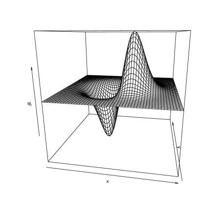
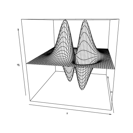
Figure 1: The influence function for the first component of the minimum pseudodistance estimator of the mean (left hand side) and the influence function for the ex diagonal component of the minimum pseudodistance estimator of the covariance matrix (right hand side). $P_{0}$ is the bivariate standard normal law and $\alpha=0.5$

We note that the solutions of the system given by (3.6) and (3.7), when $w_{1},w_{2},w_{3}$ are arbitrary weight functions, define statistical functionals of general M-estimators of $(\mu,\Sigma)$ (see Huber (1977), Jaupi and Saporta (1993)). According to the results presented by Jaupi and Saporta (1993), the influence functions for general M-estimators of $\mu$ and $\Sigma$ are given by

$$\mathrm{IF}(x;\mu,P_{\mu,\Sigma}) = (x-\mu)w_{\mu}(\|x-\mu\|_{\Sigma^{-1}})$$ (3.9)

$$\mathrm{IF}(x;\Sigma,P_{\mu,\Sigma}) = (x-\mu)(x-\mu)^{t}w_{\eta}(\|x-\mu\|_{\Sigma^{-1}})-\Sigma w_{\delta}(\|x-\mu\|_{\Sigma^{-1}})$$ (3.10)

where

$$w_{\mu}(\|x-\mu\|_{\Sigma^{-1}}) = \frac{w_{1}(\|x-\mu\|_{\Sigma^{-1}})}{E_{P_{0}}\left[w_{1}(\|y\|)+\frac{1}{N}w_{1}^{\prime}(\|y\|)\|y\|\right]}$$

$$w_{\eta}(\|x-\mu\|_{\Sigma^{-1}}) = \frac{N(N+2)w_{2}(\|x-\mu\|_{\Sigma^{-1}})}{\|x-\mu\|^{2}_{\Sigma^{-1}}E_{P_{0}}\left[Nw_{2}(\|y\|)+w_{2}^{\prime}(\|y\|)\|y\|\right]}$$

$$w_{\delta}(\|x-\mu\|_{\Sigma^{-1}}) = \frac{Nw_{3}(\|x-\mu\|_{\Sigma^{-1}})-2w_{2}(\|x-\mu\|_{\Sigma^{-1}})}{E_{P_{0}}\left[w_{2}^{\prime}(\|y\|)\|y\|-Nw_{3}^{\prime}(\|y\|)\|y\|\right]}+$$

$$+\frac{(N+2)w_{2}(\|x-\mu\|_{\Sigma^{-1}})}{E_{P_{0}}\left[Nw_{2}(\|y\|)+w_{2}^{\prime}(\|y\|)\|y\|\right]}$$

$P_{0}$ denoting the probability measure associate to the $N$-variate standard normal distribution and $\|\cdot\|$ the Euclidian norm.

For the weight functions $w_{1},w_{2},w_{3}$ from (3.8), corresponding to the minimum pseudodistance estimators, we get

$$w_{\mu}(t) = (\sqrt{\alpha+1})^{N+2}\exp\left(-\frac{\alpha}{2}t^{2}\right)$$ (3.11)

$$w_{\eta}(t) = (\sqrt{\alpha+1})^{N+4}\exp\left(-\frac{\alpha}{2}t^{2}\right)$$ (3.12)

$$w_{\delta}(t) = (\sqrt{\alpha+1})^{N+2}\exp\left(-\frac{\alpha}{2}t^{2}\right)$$ (3.13)

and replacing in (3.9) and in (3.10) we obtain

$$\mathrm{IF}(x;\mu,P_{\mu,\Sigma}) = (\sqrt{\alpha+1})^{N+2}(x-\mu)\exp\left(-\frac{\alpha}{2}\|x-\mu\|^{2}_{\Sigma^{-1}}\right)$$ (3.14)

$$\mathrm{IF}(x;\Sigma,P_{\mu,\Sigma}) = (\sqrt{\alpha+1})^{N+4}\left[(x-\mu)(x-\mu)^{t}-\frac{1}{\alpha+1}\Sigma\right]\exp\left(-\frac{\alpha}{2}\|x-\mu\|^{2}_{\Sigma^{-1}}\right).$$ (3.15)

Both influence functions are bounded with respect to $x$. Therefore the minimum pseudodistance estimators of $\mu$ and $\Sigma$ are robust. In Figure 1 we represent the influence function for the first component of the minimum pseudodistance estimator of the mean, respectively the influence function for the ex diagonal component of the minimum pseudodistance estimator of the covariance matrix. For both representations, we considered $P_{0}$ the bivariate standard normal low and we chosed $\alpha=0.5$.

3.4 Asymptotic normality

For general parametric models, the minimum pseudodistance estimators are asymptotically normal distributed (see Broniatowski et al. (2012)). In this section, we derive the asymptotic covariance matrices of the mean and the covariance matrix minimum pseudodistance estimators. We adopt the influence function approach and make use of the general results for affine equivariant location and dispersion M-estimators as presented in Gervini (2002) and Hampel et al. (1986).

When the observations correspond to the standard $N$-variate normal law $P_{0}$, under appropriate conditions, $\widehat{\mu}$ is asymptotically normal distributed with the asymptotic covariance matrix

$$V(\mu,P_{0})=\mathrm{E}_{P_{0}}\{\mathrm{IF}(Z;\mu,P_{0})\mathrm{IF}(Z;\mu,P_{0})^{t}\}=d_{\mu}I$$ (3.16)

where $d_{\mu}:=\mathrm{E}_{P_{0}}\{\|Z\|^{2}w_{\mu}^{2}(\|Z\|)\}/N$ and $I$ is the identity matrix. Formula (3.16) has been established by Gervini (2002) for general affine equivariant location M-estimators. The estimator $\widehat{\mu}$ belongs to this class. For the weight $w_{\mu}$ from (3.11) we get $d_{\mu}=(\alpha+1)^{N+2}/(\sqrt{2\alpha+1})^{N+2}$, hence the asymptotic covariance matrix of the minimum pseudodistance estimator $\widehat{\mu}$ is

$$V(\mu,P_{0})=\frac{(\alpha+1)^{N+2}}{(\sqrt{2\alpha+1})^{N+2}}I.$$

When the observations correspond to the normal law $P_{\mu,\Sigma}$, the asymptotic covariance matrix of $\widehat{\mu}$ is given by

$$V(\mu,P_{\mu,\Sigma})=E_{P_{\mu,\Sigma}}\{\mathrm{IF}(X;\mu,P_{\mu,\Sigma})\mathrm{IF}(X;\mu,P_{\mu,\Sigma})^{t}\}=d_{\mu}\Sigma=\frac{(\alpha+1)^{N+2}}{(\sqrt{2\alpha+1})^{N+2}}\Sigma.$$ (3.17)

Similar results hold for $\mathrm{vecs}(\widehat{\Sigma})$, where $\mathrm{vecs}$ is the operation that stacks the $N+N(N-1)/2$ non-redundant elements of $\Sigma$ into a vector, as follows: $\mathrm{vecs}(\Sigma):=(\sigma_{11}/\sqrt{2},\dots,\sigma_{NN}/\sqrt{2},\sigma_{21},\sigma_{31},\dots,\sigma_{N,N-1})^{t}$. According to the results of Gervini (2002), when the observations come from the $N$-variate standard normal law $P_{0}$, the asymptotic covariance matrix corresponding to an affine equivariant M-estimator of the covariance matrix is given by

$$V(\Sigma,P_{0}) = \mathrm{E}_{P_{0}}\{\mathrm{vecs}\mathrm{IF}(Z;\Sigma,P_{0})\mathrm{vecs}\mathrm{IF}(Z;\Sigma,P_{0})^{t}\}$$

$$= d_{\eta}(I-\frac{1}{N}ww^{t})+d_{\tau}\cdot\frac{1}{N}ww^{t}$$

where $w^{t}:=(e^{t}_{N},\mathbf{0}_{N(N-1)/2}^{t})$, $d_{\eta}:=\mathrm{E}_{P_{0}}\{\|Z\|^{4}w_{\eta}^{2}(\|Z\|)\}/(N(N+2))$ and $d_{\tau}:=\mathrm{E}_{P_{0}}\{w_{\tau}^{2}(\|Z\|)\}/(2N)$ with $w_{\tau}:=t^{2}w_{\eta}(t)-Nw_{\delta}(t)$, $w_{\eta}$, $w_{\delta}$ and $w_{\tau}$ being specific to the M-estimator in question.

In our case, $w_{\eta}$ and $w_{\delta}$ are given by (3.12) and (3.13), hence

$$w_{\tau}(t)=(\sqrt{\alpha+1})^{N+4}\left[t^{2}-\frac{N}{\alpha+1}\right]\exp\left(-\frac{\alpha}{2}t^{2}\right).$$

After some calculation, we obtain

$$d_{\eta}=\left(\frac{\alpha+1}{\sqrt{2\alpha+1}}\right)^{N+4}\;\text{and}\;d_{\tau}=\frac{N\alpha^{2}(\alpha+1)^{N+2}}{2(\sqrt{2\alpha+1})^{N+4}}+\left(\frac{\alpha+1}{\sqrt{2\alpha+1}}\right)^{N+4},$$

therefore,

$$V(\Sigma,P_{0})=\left(\frac{\alpha+1}{\sqrt{2\alpha+1}}\right)^{N+4}I+\frac{\alpha^{2}(\alpha+1)^{N+2}}{2(\sqrt{2\alpha+1})^{N+4}}ww^{t}.$$ (3.18)

When the observations correspond to the law $P_{\mu,\Sigma}$, the asymptotic covariance matrix of $\mathrm{vecs}(\widehat{\Sigma})$ can be established by using the formula from Hampel et al. (1986) p.282, which in our notations writes as follows

$$V(\Sigma,P_{\mu,\Sigma})=\left[\frac{\partial[\Sigma^{\frac{1}{2}}S\Sigma^{\frac{1}{2}}]}{\partial\mathrm{vecs}S}\right]V(\Sigma,P_{0})\left[\frac{\partial[\Sigma^{\frac{1}{2}}S\Sigma^{\frac{1}{2}}]}{\partial\mathrm{vecs}\Sigma}\right]^{t}.$$ (3.19)

According to Hampel et al. (1986) p.272, for a given $N\times N$ matrix $\Sigma_{*}$, it holds

$$\left[\frac{\partial[\Sigma^{\frac{1}{2}}S\Sigma^{\frac{1}{2}}]}{\partial\mathrm{vecs}S}\right]\mathrm{vecs}\Sigma_{*}=\mathrm{vecs}(\Sigma^{\frac{1}{2}}\Sigma_{*}\Sigma^{\frac{1}{2}}).$$

Particularly,

$$\left[\frac{\partial[\Sigma^{\frac{1}{2}}S\Sigma^{\frac{1}{2}}]}{\partial\mathrm{vecs}S}\right]\mathrm{vecs}I=\mathrm{vecs}\Sigma.$$ (3.20)

Note that $w=\sqrt{2}\mathrm{vecs}I$ and combining (3.19), (3.18) and (3.20), we get

$$V(\Sigma,P_{\mu,\Sigma})=\left(\frac{\alpha+1}{\sqrt{2\alpha+1}}\right)^{N+4}\left[\frac{\partial[\Sigma^{\frac{1}{2}}S\Sigma^{\frac{1}{2}}]}{\partial\mathrm{vecs}S}\right]\left[\frac{\partial[\Sigma^{\frac{1}{2}}S\Sigma^{\frac{1}{2}}]}{\partial\mathrm{vecs}S}\right]^{t}+\frac{\alpha^{2}(\alpha+1)^{N+2}}{(\sqrt{2\alpha+1})^{N+4}}\mathrm{vecs}\Sigma(\mathrm{vecs}\Sigma)^{t}.$$

For symmetry reasons, the minimum pseudodistance location and covariance estimators are asymptotically uncorrelated and hence asymptotically independent. This is valid for location and covariance M-estimators in general, as it is underlined in various articles, for example in Huber (1977).

3.5 Asymptotic relative efficiency

In order to assess the efficiency of the proposed estimators with respect to that of the MLE, we adopt as measure the asymptotic relative efficiency (ARE). For a parameter $\theta$ taking values in $\mathbb{R}^{d}$ and an estimator $\widehat{\theta}$ which is asymptotically $d$-variate normal with mean $\theta$ and nonsingular covariance matrix $V(\theta,P)$, the asymptotic relative efficiency with respect to that of the MLE is defined as

$$\mathrm{ARE}(\widehat{\theta},P)=\left(\frac{\det V_{0}(\theta,P)}{\det V(\theta,P)}\right)^{1/d},$$

$V_{0}(\theta,P)$ being the asymptotic covariance matrix of the MLE of $\theta$ when the observations follow the law $P$ (see Serfling (2011)). Although the asymptotically most efficient estimator is given by the MLE, the particular MLE can be drastically inefficient when the underlying distribution departs even a little bit from the assumed nominal distribution. Therefore the trade-off between robustness and efficiency should be carefully analyzed.

Due to the asymptotic independence of the mean and the covariance matrix minimum pseudodistance estimators, the asymptotic relative efficiency of $\widehat{\theta}=(\widehat{\mu}^{t},\mathrm{vecs}(\widehat{\Sigma})^{t})^{t}$ can be expressed as

$$\mathrm{ARE}(\widehat{\theta},P_{\mu,\Sigma})=\left(\frac{\det V_{0}(\theta,P_{\mu,\Sigma})}{\det V(\theta,P_{\mu,\Sigma})}\right)^{\frac{2}{N(N+3)}}=\left(\frac{\det V_{0}(\mu,P_{\mu,\Sigma})\det V_{0}(\Sigma,P_{\mu,\Sigma})}{\det V(\mu,P_{\mu,\Sigma})\det V(\Sigma,P_{\mu,\Sigma})}\right)^{\frac{2}{N(N+3)}}.$$ (3.21)

Using (3.17) and (3.19), formula (3.21) can be written as

$$\mathrm{ARE}(\widehat{\theta},P_{\mu,\Sigma})=\left(\frac{\det V_{0}(\mu,P_{0})\det V_{0}(\Sigma,P_{0})}{\det V(\mu,P_{0})\det V(\Sigma,P_{0})}\right)^{\frac{2}{N(N+3)}}.$$

A direct calculation shows that

$$\det V(\mu,P_{0}) = \left(\frac{\alpha+1}{\sqrt{2\alpha+1}}\right)^{N(N+2)}$$

$$\det V(\Sigma,P_{0}) = \left(\frac{\alpha+1}{\sqrt{2\alpha+1}}\right)^{\frac{N(N+1)(N+4)}{2}}\left(1+\frac{N\alpha^{2}}{2(\alpha+1)^{2}}\right).$$

Particularly, for $\alpha=0$, we find the similar quantities for the MLE, namely $\det V_{0}(\mu,P_{0})=1$ and $\det V_{0}(\Sigma,P_{0})=1$. Hence

$$\mathrm{ARE}(\widehat{\theta},P_{\mu,\Sigma})=\frac{1}{\left(\frac{\alpha+1}{\sqrt{2\alpha+1}}\right)^{\frac{N^{2}+7N+8}{N+3}}\left(1+\frac{N\alpha^{2}}{2(\alpha+1)^{2}}\right)^{\frac{2}{N(N+3)}}}.$$ (3.22)

Note that, for fixed $N$ and $\alpha$, $\mathrm{ARE}(\widehat{\theta},P_{\mu,\Sigma})$ is the same, whatever $\mu$ or $\Sigma$.

N	$\alpha=0$	$\alpha=0.1$	$\alpha=0.2$	$\alpha=0.5$	$\alpha=0.75$	$\alpha=1$
1	1	0.98151	0.93871	0.76904	0.63774	0.53033
2	1	0.97704	0.92429	0.72086	0.57042	0.45266
3	1	0.97273	0.91051	0.67698	0.51187	0.38814
4	1	0.96851	0.89718	0.63647	0.46018	0.33370
5	1	0.96435	0.88419	0.59879	0.41420	0.28738
6	1	0.96025	0.87148	0.56360	0.37311	0.24778
7	1	0.95619	0.85902	0.53065	0.33629	0.21380
8	1	0.95215	0.84679	0.49975	0.30322	0.18460
9	1	0.94815	0.83477	0.47073	0.27350	0.15946
10	1	0.94418	0.82294	0.44345	0.24674	0.13779

Table 1: Asymptotic relative efficiency of the minimum pseudodistance estimators

In Table 1 values of the asymptotic relative efficiency (3.22) are given. As it can be seen, when $N$ or $\alpha$ increases, the asymptotic relative efficiency $\mathrm{ARE}(\widehat{\theta},P_{\mu,\Sigma})$ decreases. Therefore, values of $\alpha$ close to zero will provide high efficiency and in the meantime the robustness of the estimation procedure.

4 The estimator of the optimal portfolio weights

We consider the estimator $\widehat{p^{*}}$ of the optimal portfolio weights, as given by (2.2), with $\widehat{\mu}$ and $\widehat{\Sigma}$ minimum pseudodistance estimators.

The influence function of the estimator $\widehat{p^{*}}$ is proportional to the influence functions of the estimators $\widehat{\mu}$ and $\widehat{\Sigma}$. More precisely,

$$\mathrm{IF}(x;p^{*},P_{\mu,\Sigma}) = -\Sigma^{-1}\mathrm{IF}(x;\Sigma,P_{\mu,\Sigma})p^{*}+\frac{1}{\lambda}\Sigma^{-1}\left\{\mathrm{IF}(x;\mu,P_{\mu,\Sigma})+\right.$$ (4.1)

$$+\frac{e_{N}^{t}\Sigma^{-1}[\mathrm{IF}(x;\Sigma,P_{\mu,\Sigma})\Sigma^{-1}\mu-\mathrm{IF}(x;\mu,P_{\mu,\Sigma})]e_{N}}{e_{N}^{t}\Sigma^{-1}e_{N}}+$$

$$\left.+\frac{(e_{N}^{t}\Sigma^{-1}\mathrm{IF}(x;\Sigma,P_{\mu,\Sigma})\Sigma^{-1}e_{N})(e_{N}^{t}\Sigma^{-1}\mu-\lambda)e_{N}}{(e_{N}^{t}\Sigma^{-1}e_{N})^{2}}\right\}$$

where $\mathrm{IF}(x;\mu,P_{\mu,\Sigma})$ and $\mathrm{IF}(x;\Sigma,P_{\mu,\Sigma})$ are those from (3.14) and (3.15). This formula is obtained by considering the statistical functional associated to the optimal portfolio weights,

$$p^{*}(P)=\frac{1}{\lambda}\Sigma^{-1}(P)\left[\mu(P)-\frac{e_{N}^{t}\Sigma^{-1}(P)\mu(P)-\lambda}{e_{N}^{t}\Sigma^{-1}(P)e_{N}}e_{N}\right]$$

where $\Sigma^{-1}(P)$ denotes the statistical functional corresponding to $\widehat{\Sigma}^{-1}$, and then deriving the influence function, taking also into account that

$$\mathrm{IF}(x;\Sigma^{-1},P_{\mu,\Sigma})=-\Sigma^{-1}\mathrm{IF}(x;\Sigma,P_{\mu,\Sigma})\Sigma^{-1}.$$

On the basis of the direct proportionality between the influence function $\mathrm{IF}(x;p^{*},P_{\mu,\Sigma})$ and the influence functions $\mathrm{IF}(x;\mu,P_{\mu,\Sigma})$ and $\mathrm{IF}(x;\Sigma,P_{\mu,\Sigma})$, we deduce that the global robustness of $\widehat{\mu}$ and $\widehat{\Sigma}$ is transferred to the plug-in estimator $\widehat{p^{*}}$.

On the other hand, by using the multivariate Delta method, the asymptotic normality of $\widehat{p^{*}}$ is kept, as well. Given the i.i.d. observations $X^{1},\dots,X^{T}$ from $P_{\mu,\Sigma}$, since $\widehat{\mu}$ and $\mathrm{vecs}(\widehat{\Sigma})$ are asymptotically normal and the function

$$h(\theta)=\frac{1}{\lambda}\Sigma^{-1}(\mu-\eta e_{N})$$

with $\theta=(\mu^{t},(\mathrm{vecs}\Sigma)^{t})^{t}$ is differentiable, by applying the multivariate Delta method, it holds

$$\sqrt{n}(\widehat{p^{*}}-p^{*})\to\mathcal{N}(0,V(p^{*},P_{\mu,\Sigma}))$$

where $V(p^{*},P_{\mu,\Sigma})=\mathrm{D}h(\theta)V(\theta,P_{\mu,\Sigma})\mathrm{D}h(\theta)^{t}$, $\mathrm{D}h(\theta)$ being the differential of $h$ in $\theta$ and

$$V(\theta,P_{\mu,\Sigma})=\begin{pmatrix}V(\mu,P_{\mu,\Sigma})&0\\ 0&V(\Sigma,P_{\mu,\Sigma})\end{pmatrix}.$$

5 Monte Carlo simulations

We performed Monte Carlo simulations in order to assess the performance of the minimum pseudodistance estimators of the mean and covariance matrix, for both contaminated and non-contaminated data. In this study, we considered the multivariate normal distribution $\mathcal{N}_{N}(\mu_{0},\Sigma_{0})$, with $\mu_{0}=\mathbf{0}$ and $\Sigma_{0}$ a $N\times N$ matrix with variances equal to 1 and covariances all equal to 0.2. We generated samples of size $T$ in which about $(1-\varepsilon)T$ observations are from $\mathcal{N}_{N}(\mu_{0},\Sigma_{0})$, while a smaller portion $\varepsilon T$ is from the contaminating distribution $\mathcal{N}_{N}(\mu_{c},\Sigma_{c})$ with $\mu_{c}=\mathbf{-4}$ and $\Sigma_{c}=4\Sigma_{0}$. We considered $N\in\{2,5,10,20\}$ and $\varepsilon\in\{0,0.05,0.1,0.2\}$. For each setting, we generated 1000 samples and for each sample we computed minimum pseudodistance estimates $\widehat{\mu}$ and $\widehat{\Sigma}$ corresponding to $\alpha\in\{0,0.1,0.2,0.5,0.75,1\}$.

The estimates $\widehat{\mu}$ and $\widehat{\Sigma}$, which are solutions of the system of equations (3.2) and (3.3), were obtained using the following reweighting algorithm.

Let $s\in\{0,1,\dots,s^{*}\}$ denotes the iteration step.

1. If $s=0$

$\mu^{(s)}$ and $\Sigma^{(s)}$ are set to be initial estimates of location and scale;

2. For $0<s<s^{*}$,

$$\mu^{(s)} = \sum_{i=1}^{T}w_{i}^{(s-1)}X^{i}$$

$$\Sigma^{(s)} = \sum_{i=1}^{T}(\alpha+1)w_{i}^{(s-1)}(X^{i}-\mu^{(s)})(X^{i}-\mu^{(s)})^{t}$$

where

$$w_{i}^{(s)}=\frac{\exp\left(-\frac{\alpha}{2}(X^{i}-\mu^{(s)})^{t}(\Sigma^{(s)})^{-1}(X^{i}-\mu^{(s)})\right)}{\sum_{i=1}^{T}\exp\left(-\frac{\alpha}{2}(X^{i}-\mu^{(s)})^{t}(\Sigma^{(s)})^{-1}(X^{i}-\mu^{(s)})\right)}.$$

At step 1, we used maximum likelihood estimates as initial estimates of location and covariance. For details on general convergence behavior of reweighting algorithms we refer to Arslan (2004). If $\alpha>0$, the above procedure associates low weights to the observations that disagree sensibly with the model. If $\alpha=0$, all the observations receive the same weight and the estimators are the maximum likelihood ones, defined through

$$\widehat{\mu}_{ML} = \frac{1}{T}\sum_{i=1}^{T}X^{i}$$

$$\widehat{\Sigma}_{ML} = \frac{1}{T}\sum_{i=1}^{T}(X^{i}-\widehat{\mu}_{ML})(X^{i}-\widehat{\mu}_{ML})^{t}.$$

				$\varepsilon=0\%$
N		$\alpha=0$	$\alpha=0.1$	$\alpha=0.2$	$\alpha=0.5$	$\alpha=0.75$	$\alpha=1$
2		0.343	0.358	0.384	0.559	0.804	1.177
5		0.513	0.530	0.593	1.340	4.806	5.324
10		0.760	0.817	0.945	10.471	11.389	12.197
20		1.290	1.429	2.069	29.979	38.830	47.064
				$\varepsilon=5\%$
N		$\alpha=0$	$\alpha=0.1$	$\alpha=0.2$	$\alpha=0.5$	$\alpha=0.75$	$\alpha=1$
2		4.425	0.888	0.533	0.593	0.849	1.202
5		18.816	1.077	0.662	1.565	4.985	5.437
10		41.312	0.951	1.022	10.646	11.470	12.600
20		145.172	1.517	2.273	30.339	39.561	47.072
				$\varepsilon=10\%$
N		$\alpha=0$	$\alpha=0.1$	$\alpha=0.2$	$\alpha=0.5$	$\alpha=0.75$	$\alpha=1$
2		11.554	4.605	0.945	0.694	0.923	1.294
5		43.446	4.075	0.749	1.758	5.052	5.449
10		143.395	1.325	1.091	10.720	11.454	12.648
20		503.319	1.648	2.422	30.776	39.758	47.693
				$\varepsilon=20\%$
N		$\alpha=0$	$\alpha=0.1$	$\alpha=0.2$	$\alpha=0.5$	$\alpha=0.75$	$\alpha=1$
2		32.696	24.612	9.955	1.118	1.190	1.475
5		132.542	53.841	1.869	2.171	5.362	5.625
10		441.209	19.233	1.241	10.751	11.751	12.745
20		1613.373	1.930	3.742	31.361	40.292	49.644

Table 2: Simulation based estimates of the mean square error, when $T=10N$

				$\varepsilon=0\%$
N		$\alpha=0$	$\alpha=0.1$	$\alpha=0.2$	$\alpha=0.5$	$\alpha=0.75$	$\alpha=1$
2		0.035	0.035	0.039	0.051	0.067	0.084
5		0.050	0.052	0.057	0.087	0.135	0.204
10		0.075	0.081	0.093	0.185	0.395	8.703
20		0.129	0.142	0.181	0.910	28.127	31.790
				$\varepsilon=5\%$
N		$\alpha=0$	$\alpha=0.1$	$\alpha=0.2$	$\alpha=0.5$	$\alpha=0.75$	$\alpha=1$
2		2.504	0.304	0.076	0.060	0.068	0.092
5		10.863	0.207	0.066	0.092	0.136	0.217
10		37.549	0.129	0.100	0.191	0.409	9.329
20		136.364	0.157	0.194	0.891	28.354	33.200
				$\varepsilon=10\%$
N		$\alpha=0$	$\alpha=0.1$	$\alpha=0.2$	$\alpha=0.5$	$\alpha=0.75$	$\alpha=1$
2		8.910	2.493	0.285	0.066	0.073	0.096
5		39.015	2.203	0.089	0.098	0.142	0.240
10		133.655	0.404	0.107	0.207	0.474	9.746
20		493.386	0.182	0.203	1.249	28.467	33.925
				$\varepsilon=20\%$
N		$\alpha=0$	$\alpha=0.1$	$\alpha=0.2$	$\alpha=0.5$	$\alpha=0.75$	$\alpha=1$
2		28.470	18.606	7.524	0.106	0.102	0.115
5		124.702	44.374	0.327	0.113	0.168	0.272
10		429.087	17.016	0.128	0.232	0.592	10.423
20		1576.600	0.335	0.229	3.460	29.091	34.815

Table 3: Simulation based estimates of the mean square error, when $T=100N$

We present simulation based estimates of the mean square error given by

$$\widehat{\mathrm{MSE}}=\frac{1}{n_{s}}\sum_{i=1}^{n_{s}}\|\widehat{\theta}_{i}-\theta_{0}\|^{2}$$

where $n_{s}$ is the number of samples (in our case $n_{s}=1000$), $\theta_{0}=(\mu_{0}^{t},\mathrm{vech}(\Sigma_{0})^{t})^{t}$ and $\widehat{\theta}_{i}=(\widehat{\mu}_{i}^{t},\mathrm{vech}(\widehat{\Sigma}_{i})^{t})^{t}$ is an estimation corresponding to the sample $i$. Here $\mathrm{vech}(\Sigma)$ is “the vector half”, namely the $n(n+1)/2$-dimensional column vector obtained by stacking the columns of the lower triangle of $\Sigma$, including the diagonal, one below the other. Table 2 and Table 3 present simulation based estimates of the mean square error, when the sample size is $T=10N$, respectively when $T=100N$. When there is no contamination, the MLE ($\alpha=0$) performs the best, whatever the dimension $N$. On the other hand, the estimations obtained with the minimum pseudodistance estimators in this case are close to those provided by MLE, when $\alpha$ is not far to zero (for example $\alpha=0.1$ and $\alpha=0.2$). In the presence of contamination, the minimum pseudodistance estimators give much better results than the MLE, in all considered cases. In most cases, the choice $\alpha=0.2$ provides the best results in terms of robustness. In the meantime, this choice corresponds to an estimation procedure with high asymptotic relative efficiency, according to the results from Table 1. These facts recommend $\alpha=0.2$ as a good choice in terms of trade-off robustness efficiency. When the contamination is more pronounced, i.e. $\varepsilon=10\%$ or $\varepsilon=20\%$, and the dimension $N$ is low, i.e. $N=2$, the choices $\alpha=0.5$, $\alpha=0.75$ or even $\alpha=1$ provide better robust estimates, but the asymptotic relative efficiencies of the corresponding estimation procedures are unacceptably low. Thus, values of $\alpha$ close to zero, such as $\alpha=0.1$, $\alpha=0.2$, represent choices that offer an equilibrium between robustness and efficiency. The simulation results presented in Table 2 and Table 3 shows that increasing sample size leads to improved estimations.

Figure 2: Boxplots for monthly log-returns corresponding to the MSCI Indexes (1: France, 2: Germany, 3: Italy, 4: Japan, 5: Pacific ex JP, 6: Spain, 7: United Kingdom, 8: USA)

6 Application for financial data

We analyze 172 monthly log-returns of 8 MSCI Indexes (France, Germany, Italy, Japan, Pacific Ex JP, Spain, United Kingdom and USA) from January 1998 to April 2012 with the aim to construct robust and efficient portfolios. The data are provided by MSCI (www.msci.com). Boxplots for these data are presented in Figure 2.

For these indexes, estimates of the expected return and of the variance are represented in Figure 4. Note that the estimates of the expected returns obtained with the minimum pseudodistance estimators are larger than the maximum likelihood ones. In the meantime, the minimum pseudodistance estimates of the variances are smaller than those provided by the MLE.

Estimates of the mean vector and of the covariance matrix computed with different minimum pseudodistance estimators are used to determine efficient frontiers. In Figure 4 we plot efficient frontiers for the case “short selling allowed”, respectively for the case “short selling not allowed”. In both cases, the frontiers based on the minimum pseudodistance estimations dominate those based on the classical maximum likelihood estimations, yielding portfolios with larger expected returns and smaller risks. Thus, the robust estimates reduce the volatility effects which typically affects the results of the traditional approaches.

The next step in our analysis is to identify the influential observations which are responsible for the shift of the efficient frontier. We perform this study in the case “short selling”. In this sense, we use the data influence measure (DIM) as diagnostic tool (see Perret-Gentil and Victoria-Feser (2005)). This is defined as the Euclidian norm of the influence function of the estimator of weights based on maximum likelihood estimators of $\mu$ and $\Sigma$. More precisely,

$$\mathrm{DIM}(x,\widehat{p^{*}})=[\mathrm{IF}(x;p^{*},P_{\mu,\Sigma})^{t}\mathrm{IF}(x;p^{*},P_{\mu,\Sigma})]^{1/2}$$

where $\mathrm{IF}(x;p^{*},P_{\mu,\Sigma})$ is given by (4.1) with $\mathrm{IF}(x;\mu,P_{\mu,\Sigma})$ and $\mathrm{IF}(x;\Sigma,P_{\mu,\Sigma})$ given by the formulas (3.14) and (3.15) in the case $\alpha=0$. In order to compute $\mathrm{DIM}$, the true parameters values $\mu,\Sigma,p^{*}$ have to be known. In practice, these parameters should be estimated in a robust way, such that DIM is not affected by the outlying observations it is supposed to detect.

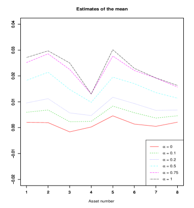
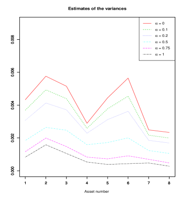
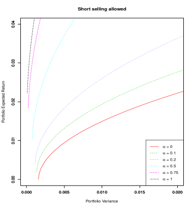
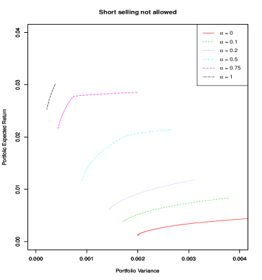
Figure 3: Expected returns estimates (left) and variance estimates (right) for the 8 MSCI Indexes (1: France, 2: Germany, 3: Italy, 4: Japan, 5: Pacific ex JP, 6: Spain, 7: United Kingdom, 8: USA)

Figure 4: Mean-variance efficient frontiers

In Figure 5 (left hand side) we represent the influence of each of the 172 observations on the estimator of the optimal portfolio weights based on maximum likelihood estimators of $\mu$ and $\Sigma$. Since $\mathrm{DIM}$ is related to a specific portfolio on the efficient frontier, we made a choice, namely the level of the portfolio variance has been set to 0.005. The necessary robust estimates of $\mu,\Sigma,p^{*}$ have been obtained with minimum pseudodistance estimators corresponding to $\alpha=0.2$. The most influential observations as detected by DIM correspond to negative economic events associated with known financial crisis periods: 1998 Russian financial crisis (August 1998), “dot-com crash” of 2000-2002 and 2007-2012 global financial crisis. On the other hand, the influence of these observations is substantially reduced when using robust procedures. This can be seen in the right hand side of Figure 5 where we represent the influence of each of the 172 observations on the robust estimator of the optimal portfolio weights based on the minimum pseudodistance estimators of $\mu$ and $\Sigma$ corresponding to $\alpha=0.2$. Reducing the influence of outlying observations leads to optimal portfolios with higher returns and smaller variances.

Our theoretical and numerical results show that the optimal portfolios based on minimum pseudodistance estimators are more robust to extreme events than those obtained by plugging-in the MLEs. When $\alpha$ is not far from 0, the minimum pseudodistance estimators of $\mu$ and $\Sigma$ combine robustness with high efficiency and these qualities are transferred to the portfolio weights estimator. The numerical results based on simulations or real data show that $\alpha=0.2$ represents a good choice in terms of robustness and efficiency. All these recommend the new procedure as a viable alternative to existing robust portfolio selection methods.

Figure 5: The influence of each of the 172 observations on the classical estimator of optimal portfolio weights (left hand side), respectively on the robust estimator of optimal portfolio weights (right hand side), as measured by DIM. The portfolio variance has been set to 0.005.

References

- [1] Arslan, O. (2004). Convergence behavior of an iterative reweighting algorithm to compute multivariate M-estimates for location and scatter. Journal of Statistical Planning and Inference, 118, 115-128.
- [2] Basu, A., Harris, I.R., Hjort, N.L., & Jones, M.C. (1998). Robust and efficient estimation by minimizing a density power divergence. Biometrika, 85, 549-559.
- [3] Broniatowski, M., & Keziou, A. (2009). Parametric estimation and tests through divergences and the duality technique. J. Multiv. Anal., 100, 16-36.
- [4] Broniatowski, M., Toma, A., & Vajda, I. (2012). Decomposable pseudodistances and applications in statistical estimation. Journal of Statistical Planning and Inference, 142, 2574-2585.
- [5] DeMiguel, V., & Nogales, F.J. (2009). Portfolio selection with robust estimation. Operations Research, 57, 560-577.
- [6] Fabozzi, F.J., Huang, D., & Zhou, G. (2010). Robust portfolios: contributions from operations research and finance. Ann. Oper. Res., 176, 191-220.
- [7] Ferrari, D., & Paterlini, S. (2010). Efficient and robust estimation for financial returns: an approach based on -entropy. Materiali di discussione, no. 623, Universita degli Studi di Modena e Reggio Emilia.
- [8] Gervini, D. (2002). The influence function of the Stahel-Donoho estimator of multivariate location and scatter. Statistics & Probability Letters, 60, 425-435.
- [9] Grossi, L., & Laurini, F., (2011). Robust estimation of efficient mean-variance frontiers. Adv. Data Anal. Classif., 5, 3-22.
- [10] Hampel, F.R., Ronchetti, E., Rousseeuw, P.J., & Stahel, W. (1986). Robust statistics: the approach based on influence functions. New York: Wiley.
- [11] Huber, P.J. (1977). Robust covariances. In S. Gupta, & D. Moore (Eds.), Statistical decision theory and related topics II.
- [12] Jaupi, L., & Saporta, G. (1993). Using the influence function in robust principal component analysis. In S. Morgenthaler, E. Ronchetti, & W.A. Stahel (Eds.), New directions in statistical data analysis and robustness (pp. 147-156). Verlag: Birchauser.
- [13] Markowitz, H.M. (1952). Mean-variance analysis in portfolio choice and capital markets. Journal of Finance, 7, 77-91.
- [14] Michaud, R. (1989). The Markowitz optimization enigma: is optimized optimal? Financ. Anal. J., 45, 31-42.
- [15] Perret-Gentil, C., & Victoria-Feser, M.P. (2005). Robust mean-variance portfolio selection. FAME Research Paper, no. 140.
- [16] Serfling, R. (2011). Asymptotic relative efficiency in estimation. In M. Lovric (Ed.), International encyclopedia of statistical sciences (pp. 68-72). New York: Springer.
- [17] Toma, A., & Broniatowski, M. (2011). Dual divergence estimators and tests: Robustness results. J. Multiv. Anal., 102, 20–36.
- [18] Toma, A., & Leoni-Aubin, S. (2010). Robust tests based on dual divergence estimators and saddlepoint approximations. J. Multiv. Anal., 101, 1143-1155.
- [19] Vaz-de Melo, B., & Camara, R.P. (2005). Robust multivariate modeling in finance. International Journal of Managerial Finance, 4, 12-23.
- [20] Welsch, R.E., & Zhou, X., 2007. Application of robust statistics to asset allocation models. RevStat, 5, 97-114.
- [21] www.msci.com