Control of a Bicycle Using Virtual Holonomic Constraints

Abstract

The paper studies the problem of making Getz’s bicycle model traverse a strictly convex Jordan curve with bounded roll angle and bounded speed. The approach to solving this problem is based on the virtual holonomic constraint (VHC) method. Specifically, a VHC is enforced making the roll angle of the bicycle become a function of the bicycle’s position along the curve. It is shown that the VHC can be automatically generated as a periodic solution of a scalar periodic differential equation, which we call virtual constraint generator. Finally, it is shown that if the curve is sufficiently long as compared to the height of the bicycle’s centre of mass and its wheel base, then the enforcement of a suitable VHC makes the bicycle traverse the curve with a steady-state speed profile which is periodic and independent of initial conditions. An outcome of this work is a proof that the constrained dynamics of a Lagrangian control system subject to a VHC are generally not Lagrangian.

1 Introduction

This paper investigates the problem of maneuvering a bicycle along a closed Jordan curve $\mathcal{C}$ in the horizontal plane in such a way that the bicycle does not fall over and its velocity is bounded. The simplified bicycle model we use in this paper, developed by Neil Getz [1, 2], views the bicycle as a point mass with a side slip velocity constraint, and models its roll dynamics as those of an inverted pendulum, see Figure 1. The model neglects, among other things, the steering kinematics and the wheels dynamics with the associated gyroscopic effect.

In [3], Hauser-Saccon-Frezza investigate the maneuvering problem for Getz’s bicycle using a dynamic inversion approach to determine bounded roll trajectories. They constrain the bicycle on the curve and, given a desired velocity signal $v(t)$, they find a trajectory with the property that the velocity of the bicycle is $v(t)$ and its roll angle $\varphi$ is in the interval $(-\pi/2,\pi/2)$, i.e, the bicycle doesn’t fall over. In [4], Hauser-Saccon develop an algorithm to compute the minimum-time speed profile for a point-mass motorcycle compatible with the constraint that the lateral and longitudinal accelerations do not make the tires slip, and apply their algorithm to Getz’s bicycle model.

The problem of maneuvering Getz’s bicycle along a closed curve is equivalent to moving the pivot point of an inverted pendulum around the curve without making the pendulum fall over. On the other hand, the seemingly different problem of maneuvering Hauser’s PVTOL aircraft [5] along a closed curve in the vertical plane can be viewed as the problem of moving the pivot of an inverted pendulum around the curve without making the pendulum fall over. The two problems are, therefore, closely related, the main difference being the fact that in the former case the pendulum lies on a plane which is orthogonal to the plane of the curve, while in the latter case it lies on the same plane. In [6], the path following problem for the PVTOL was solved by enforcing a virtual holonomic constraint (VHC) which specifies the roll angle of the PVTOL as a function of its position on the curve. In this paper we follow a similar approach for the bicycle model, and impose a VHC relating the bicycle’s roll angle to its position along the curve. However, rather than finding one VHC, as we did in [6], we show how to automatically generate VHCs as periodic solutions of a scalar periodic differential equation which we call the virtual constraint generator. We show that if the path is sufficiently long compared to the height of the bicycle’s centre of mass and the wheel base, then the VHC can be chosen so that on the constraint manifold the bicycle traverses the entire curve with bounded speed, and its speed profile is periodic in steady-state. Finally, we design a controller that enforces the VHC, and recovers the asymptotic properties of the bicycle on the constraint manifold.

\psfrag{a}{$\varphi$}\psfrag{b}{$\alpha$}\psfrag{p}{$\psi$}\psfrag{l}{$b$}\psfrag{k}{$p$}\psfrag{h}{$h$}\psfrag{m}{$m$}\psfrag{c}{$(x,y)$}\includegraphics[width=234.87749pt]{FIGURES/bicycle}

Figure 1: Getz’s bicycle model.

The concept of VHC is a promising paradigm for motion control. It is one of the central ideas in the work of Grizzle and collaborators on biped locomotion (e.g., [7] and [8]), where VHCs are used to encode different walking gaits. The work of Shiriaev and collaborators in [9, 10, 11] investigates VHCs for Lagrangian control systems, i.e., systems of the form [12]

$$\frac{d}{dt}\frac{\partial L}{\partial\dot{q}}-\frac{\partial L}{\partial q}=Gu,$$ (1)

with control input $u$ and smooth Lagrangian $L(q,\dot{q})=(1/2)\dot{q}^{\top}D(q)\dot{q}-V(q)$, with $D=D^{\top}$ positive definite. In [10], the authors consider systems of the form (1) with degree of underactuation one. They find an integral of motion for the constrained dynamics, and use it to select a desired closed orbit on the constraint manifold. This orbit is then stabilized by linearizing the control system along it, and designing a time-varying controller for the linearization. In [13], these ideas are extended to systems with degree of underactuation greater than one, and in [14] they are applied to the stabilization of oscillations in the Furuta pendulum. In [15], we investigated VHCs for Lagrangian control systems with degree of underactuation one. We introduced and characterized a notion of regularity of VHCs, and we presented sufficient conditions under which the reduced dynamics on the constraint manifold (described by a second-order unforced system) are Lagrangian (i.e., they satisfy the Euler-Lagrange equations, which have the form (1) with zero right-hand side). An outcome of this paper (Proposition 4.1) is a simple sufficient condition under which the reduced dynamics are not Lagrangian. We refer the reader to Remarks 4.3, 4.4, and 4.8 for more details.

This paper is organized as follows. In Section 2 we present Getz’s bicycle model and we formulate the maneuvering problem investigated in this paper. In Section 3 we present the virtual constraint generator idea. The main result is Proposition 3.3 which gives a constructive methodology to find VHCs for Getz’s bicycle that meet the requirements of the maneuvering problem. In Section 4 we analyze the motion of Getz’s bicycle on the virtual constraint manifold. In Proposition 4.1 we provide a general result with sufficient conditions under which an unforced second-order system of a certain form possesses an asymptotically stable closed orbit. In Proposition 4.6 we apply this result to Getz’s bicycle model. In Section 5 we bring these results together and solve the maneuvering problem. Finally, in Section 6 we make remarks on numerical implementation of the proposed controller.

Notation. Throughout this paper we use the following notation. If $x$ is a real number and $T>0$, the number $x$ modulo $T$ is denoted by $[x]_{T}$. We let $[\mathbb{R}]_{T}:=\{[x]_{T}:x\in\mathbb{R}\}$. The set $[\mathbb{R}]_{T}$ is diffeomorphic to the unit circle. We let $\pi:\mathbb{R}\to[\mathbb{R}]_{T}$ be defined as $\pi(t)=[t]_{T}$. Then, $\pi$ is a smooth covering map (see [16, p.91]). If $M$ is a smooth manifold, and $h:[\mathbb{R}]_{T}\to M$ is a smooth function, we define $\tilde{h}:=h\circ\pi:\mathbb{R}\to M$. This is a $T$-periodic function. Moreover, by [16, Theorem 4.29], $\tilde{h}$ is smooth if and only if $h$ is smooth. Finally, $\operatorname{Im}(h)$ denotes the image of a function $h$.

2 Problem formulation

Consider the bicycle model depicted in Figure 1, with the following variable conventions (taken from [3]):

• $(x,y)$ - coordinates of the point of contact of the rear wheel

• $\varphi$ - roll angle (a positive $\dot{\varphi}$ implies that the bicycle leans to the right)

• $\psi$ - yaw angle (a positive $\dot{\psi}$ means that the bicycle turns right)

• $\alpha$ - projected steering angle on the $(x,y)$ plane

• $b$ - distance between the projection of the centre of mass and the point of contact of the rear wheel

• $p$ - wheel base

• $h$ - pendulum length

• $v$ - forward linear velocity of the bicycle

• $f$ - thrust force.

We denote $\bar{\kappa}=(\tan\alpha)/p=\dot{\psi}/v$. For a given velocity signal $v(t)$ and steering angle signal $\alpha(t)$, $\bar{\kappa}(t)$ represents the curvature of the path $(x(t),y(t))$ traced by the point of contact of the rear wheel. In [2], the bicycle of Figure 1 was modelled by writing the Lagrangian of the unconstrained bicycle, incorporating the nonholonomic constraints that the wheels roll without slipping in the Lagrangian, and then extracting the model through the Lagrange-d’Alembert equations as in [12, Section 5.2]. The resulting model, which we’ll refer to as Getz’s bicycle model, reads as

$$\dot{\bar{\kappa}}=\tau$$

$$M\begin{bmatrix}\ddot{\varphi}\\ \dot{v}\end{bmatrix}=F+B\begin{bmatrix}\tau\\ f\end{bmatrix},$$ (2)

where $\tau$, the time derivative of the curvature $\bar{\kappa}(t)$, and $f$ are the control inputs and, denoting $s_{\varphi}=\sin\varphi$, $c_{\varphi}=\cos\varphi$,

$$M=\begin{bmatrix}h^{2}&bhc_{\varphi}\bar{\kappa}\\ bhc_{\varphi}\bar{\kappa}&1+(b^{2}+h^{2}s_{\varphi}^{2})\bar{\kappa}^{2}-2h{\bar{\kappa}}s_{\varphi}\end{bmatrix},$$

$$F=\begin{bmatrix}ghs_{\varphi}-(1-h{\bar{\kappa}}s_{\varphi})hc_{\varphi}{\bar{\kappa}}v^{2}\\ (1-h{\bar{\kappa}}s_{\varphi})2hc_{\varphi}{\bar{\kappa}}v\dot{\varphi}+bh{\bar{\kappa}}s_{\varphi}\dot{\varphi}^{2}\end{bmatrix},$$

$$B=\begin{bmatrix}-bhc_{\varphi}v&0\\ -(b^{2}{\bar{\kappa}}-hs_{\varphi}(1-h{\bar{\kappa}}s_{\varphi}))v&1/m\end{bmatrix}.$$

In this model, $M$ is the inertia matrix, $F$ represents the sum of Coriolis, centrifugal and conservative forces, and $B$ is the input matrix. Now consider a $C^{3}$ closed Jordan curve $\mathcal{C}$ in the $(x,y)$ plane with regular parametrization $\sigma:[\mathbb{R}]_{T}\to\mathbb{R}^{2}$, not necessarily unit speed. Let $\kappa:[\mathbb{R}]_{T}\to\mathbb{R}$ denote the signed curvature of $\mathcal{C}$. Throughout this paper, we assume the following.

Assumption 1.

The curve $\mathcal{C}$ is strictly convex, i.e., $\kappa(s)>0$ for all $s\in[\mathbb{R}]_{T}$.

In this paper we investigate the dynamics of the bicycle when the point $(x,y)$ is made to move along the curve $\mathcal{C}$ by an appropriate choice of the steering angle. In order to derive the constrained dynamics, suppose that $(x(0),y(0))\in\mathcal{C}$, i.e., $(x(0),y(0))=\sigma(s_{0})$, for some $s_{0}\in[\mathbb{R}]_{T}$. A point $\sigma(s(t))$ moving on $\mathcal{C}$ has linear velocity

$$v(t)=\|\sigma^{\prime}(s(t))\|\dot{s}(t)$$ (3)

and acceleration

$$\dot{v}(t)=\|\sigma^{\prime}(s(t))\|\ddot{s}(t)+\frac{\dot{s}^{2}(t)}{\|\sigma^{\prime}(s(t))\|}\sigma^{\prime}(s(t))^{\top}\sigma^{\prime\prime}(s(t)).$$ (4)

For an arbitrary input signal $f(t)$, $(x(t),y(t))$ traverses $\mathcal{C}$ with velocity $v(t)$ if and only if $(x(0),y(0))\in\mathcal{C}$, $(\dot{x}(0),\dot{y}(0))$ is tangent to $\mathcal{C}$, $\bar{\kappa}(0)=\kappa(s_{0})$, and the input signal $\tau(t)$ is chosen to be $\tau(t)=\kappa^{\prime}(s(t))\dot{s}(t)$, where $\kappa^{\prime}(s(t))=\frac{d\kappa}{ds}(s(t))$. With this choice, we obtain

$${\bar{\kappa}}(t)=\kappa(s(t)),$$ (5)

where $s(t)$ and $\dot{s}(t)$ are solutions of a differential equation to be specified later. The motion of the bicycle on the curve $\mathcal{C}$ is now found by substituting (3), (4), (5) and $\tau=\kappa^{\prime}(s)\dot{s}$ in (2):

$$\bar{M}\begin{bmatrix}\ddot{\varphi}\\ \|\sigma^{\prime}\|\ddot{s}+\frac{(\sigma^{\prime})^{\top}\sigma^{\prime\prime}}{\|\sigma^{\prime}\|}\dot{s}^{2}\end{bmatrix}=\bar{F}+\begin{bmatrix}0\\ 1/m\end{bmatrix}f\;,$$ (6)

where $\bar{M}=M|_{\bar{\kappa}=\kappa(s)}$ and

$$\bar{F}=\left(F+B\begin{bmatrix}1\\ 0\end{bmatrix}\kappa^{\prime}(s)\dot{s}\right)\bigg{|}_{\bar{\kappa}=\kappa(s),v=\|\sigma^{\prime}(s)\|\dot{s}}.$$

Note that we have used the control input $\tau$ to make the curve $\mathcal{C}$ invariant, so in (6) we are left with one control input, the thrust force $f$. One can check that system (6) is a Lagrangian control system with input $f$, i.e., it has the form (1) with $q=(\varphi,s)\in\mathcal{Q}=S^{1}\times[\mathbb{R}]_{T}$, $G=[0\ \ 1/m]^{\top}$, and

$$L(q,\dot{q})=\frac{1}{2}[\dot{\varphi}\ \ \|\sigma^{\prime}(s)\|\dot{s}]\bar{M}(q)\begin{bmatrix}\dot{\varphi}\\ \|\sigma^{\prime}(s)\|\dot{s}\end{bmatrix}-gh\cos\varphi.$$

Since the control force $f$ enters nonsingularly in the $\ddot{s}$ equation, we can define a feedback transformation for $f$ in (6) such that $\ddot{s}=u$, where $u$ is the new control input. With this transformation, the motion of the bicycle when its rear wheel is made by feedback control to follow $\mathcal{C}$ reads as

$$\ddot{\varphi}=h^{-1}gs_{\varphi}-h^{-1}\Big{[}(1-h\kappa(s)s_{\varphi})\kappa(s)\|\sigma^{\prime}(s)\|+b\kappa^{\prime}(s)$$ (7)

$$+\frac{b\kappa(s)}{\|\sigma^{\prime}(s)\|^{2}}{\sigma^{\prime}(s)}^{\top}\sigma^{\prime\prime}(s)\Big{]}c_{\varphi}\|\sigma^{\prime}(s)\|\dot{s}^{2}-a(s)c_{\varphi}u$$

$$\ddot{s}=u,$$

where $a(s)=bh^{-1}\kappa(s)\|\sigma^{\prime}(s)\|$. In the above equation, $u$ is the new control input, and it represents the acceleration of the curve parameter $s$. We will denote $\mathcal{X}:=\{(q,\dot{q})\in S^{1}\times[\mathbb{R}]_{T}\times\mathbb{R}^{2}\}$ the state space of (7).

Remark 2.1.

If $\sigma(s)$ is a unit speed parametrization of $\mathcal{C}$ (i.e. it satisfies $\|\sigma^{\prime}(s)\|=1$), then the first differential equation in (7) reduces to $h\ddot{\varphi}=gs_{\varphi}-\Big{[}(1-h\kappa(s)s_{\varphi})\kappa(s)+b\kappa^{\prime}(s)\Big{]}c_{\varphi}\dot{s}^{2}-b\kappa(s)c_{\varphi}u$.

Maneuvering Problem.   Find a feedback $u(q,\dot{q})$ for system (7) such that there exists a set of initial conditions $\Omega$ with the property that, for all $(q(0),\dot{q}(0))\in\Omega$, the bicycle does not overturn, i.e., $|\varphi(t)|<\pi/2$ for all $t\geq 0$, and traverses the entire curve $\mathcal{C}$ in one direction, i.e., there exists $\bar{t}>0$ such that $|\dot{s}(t)|>0$ for all $t\geq\bar{t}$. Moreover, the speed $\dot{s}(t)$ of the bicycle on $\mathcal{C}$ should remain bounded.

Our solution of this problem relies on the notion of VHC.

Definition 2.2 ([15]).

A virtual holonomic constraint (VHC) for system (7) is a relation $\varphi=\Phi(s)$, where $\Phi:[\mathbb{R}]_{T}\to S^{1}$ is smooth and the set $\Gamma=\{(q,\dot{q})\in\mathcal{X}:\varphi=\Phi(s),\ \dot{\varphi}=\Phi^{\prime}(s)\dot{s}\}$ is controlled invariant. That is, there exist a smooth feedback $u(q,\dot{q})$ such that $\Gamma$ is invariant for the closed-loop system. The set $\Gamma$ is called the constraint manifold associated with the VHC $\varphi=\Phi(s)$.

The definition above formalizes the notion of VHC used in [8] in the context of biped locomotion. The constraint manifold $\Gamma$ is a two-dimensional submanifold of $\mathcal{X}$ parametrized by $(s,\dot{s})$, and therefore diffeomorphic to the cylinder $[\mathbb{R}]_{T}\times\mathbb{R}$. It is the collection of all those phase curves of (7) that can be made to satisfy the constraint $\varphi=\Phi(s)$ via feedback control. In order to solve the maneuvering problem, we look for VHCs $\varphi=\Phi(s)$ such that $|\Phi(s)|<\pi/2$ for all $s\in[\mathbb{R}]_{T}$, and then stabilize the associated virtual constraint manifold. In [3], Hauser-Saccon-Frezza find “bounded roll trajectories,” i.e., controlled trajectories of (7) along which the roll angle $\varphi$ is bounded in the interval $(-\pi/2,\pi/2)$. In our context, each VHC $\varphi=\Phi(s)$ provides a family of bounded roll trajectories. Once $\Gamma$ has been made invariant via feedback control, bounded roll trajectories can be obtained by picking arbitrary $(s_{0},\dot{s}_{0})\in[\mathbb{R}]_{T}\times\mathbb{R}$, and picking as initial condition in (7), $(\varphi(0),s(0))=(\Phi(s_{0}),s_{0})$, $(\dot{\varphi}(0),\dot{s}(0))=(\Phi^{\prime}(s_{0})\dot{s}_{0},\dot{s}_{0})$. The resulting solution $(q(t),\dot{q}(t))$ will satisfy $\varphi(t)=\Phi(s(t))$, implying that the roll angle trajectory $\varphi(t)$ is bounded in the interval $(-\pi/2,\pi/2)$.

3 The virtual constraint generator

In this section we show that VHCs for (7) can be generated as solutions of a first-order differential equation, which we call the VHC generator. This idea was first presented in our previous work [17]. We begin with a sufficient condition for a relation $\Phi$ to be a VHC for (7).

Lemma 3.1.

A relation $\varphi=\Phi(s)$, where $\Phi:[\mathbb{R}]_{T}\to S^{1}$ is smooth, is a VHC for system (7) if

$$(\forall s\in[\mathbb{R}]_{T})\ \Phi^{\prime}(s)+a(s)\cos\Phi(s)\neq 0.$$ (8)

Proof.

Letting $H(\varphi,s):=\varphi-\Phi(s)$, condition (8) is the requirement that system (7) with output $H(\varphi,s)$ has a well-defined uniform relative degree 2 on the set $\{(q,\dot{q})\in\mathcal{X}:\varphi=\Phi(s)\}$. The associated zero dynamics manifold is precisely $\Gamma$, and it is controlled invariant. ∎

The foregoing lemma inspires the following observation. Instead of guessing a relation $\varphi=\Phi(s)$ and checking whether it is a VHC for (7), as in Lemma 3.1, we will assign a nonzero right-hand side to (8), view the resulting identity as an ODE, and generate VHCs by solving the ODE. More precisely, recall the notation $\tilde{h}:=h\circ\pi$, and consider the scalar $T$-periodic differential equation

$$\dot{x}=-\tilde{a}(t)\cos x+\tilde{\delta}(t),$$ (9)

where $\tilde{\delta}:\mathbb{R}\to\mathbb{R}\backslash\{0\}$ is a $T$-periodic function to be assigned. Then, $T$-periodic solutions of (9) give rise to VHCs.

Lemma 3.2.

Suppose that $x(t)$ is a $T$-periodic solution of (9), where $\tilde{\delta}:\mathbb{R}\to\mathbb{R}\backslash\{0\}$ is smooth and $T$-periodic. Then, the relation $\varphi=\Phi(s)$, with $\Phi:=x\circ\pi^{-1}:[\mathbb{R}]_{T}\to\mathbb{R}$, is a VHC for (7).

Proof.

Let $x(t)$ be a $T$-periodic solution of (9). Then, $x(t)$ is smooth because the right-hand side of (9) is smooth. Since $x(t)$ is $T$-periodic, $\Phi:=x\circ\pi^{-1}$ is a well-defined function $[\mathbb{R}]_{T}\to\mathbb{R}$, and by [16, Theorem 4.29] it is smooth. Since $x=\Phi\circ\pi$, we have $\dot{x}(t)=\Phi^{\prime}(\pi(t))\dot{\pi}(t)=\Phi^{\prime}(\pi(t))$, so that $\Phi^{\prime}(s)=\dot{x}(t)|_{t=\pi^{-1}(s)}$. Using (9), we get

$$\Phi^{\prime}(s) =-\tilde{a}(\pi^{-1}(s))\cos\Phi(s)+\tilde{\delta}(\pi^{-1}(s))$$

$$=-a(s)\cos\Phi(s)+\delta(s).$$ (10)

Since $\delta(s)\neq 0$ for all $s\in[\mathbb{R}]_{T}$, by Lemma 3.1 the relation $\varphi=\Phi(s)$ is a VHC for system (7). ∎

In light of Lemma 3.2, we call the differential equation (9) a VHC generator, for which one is to pick a $T$-periodic $\tilde{\delta}:\mathbb{R}\to\mathbb{R}\backslash\{0\}$ yielding a $T$-periodic solution. The next proposition shows how to pick $\tilde{\delta}$.

Proposition 3.3.

Consider the smooth and $T$-periodic differential equation (9), and set $\tilde{\delta}(t)=\epsilon\tilde{\mu}(t)$, where $\tilde{\mu}:\mathbb{R}\to(0,\infty)$ is smooth and $T$-periodic. Let $K^{+}=\max_{t\in[0,T]}[\tilde{\mu}(t)/\tilde{a}(t)]$, $K^{-}=\min_{t\in[0,T]}[\tilde{\mu}(t)/\tilde{a}(t)]$. Then, for any $x_{0}\in(0,\pi/2)$ and $t_{0}\in\mathbb{R}$, the following two properties hold:

1. there exists a unique $\epsilon\in[\epsilon^{-},\epsilon^{+}]=[(c_{x_{0}})/K^{+},$ $(c_{x_{0}})/K^{-}]$, such that the solution $x(t)$ of (9) with initial condition $x(t_{0})=x_{0}$ is $T$-periodic, and setting $\Phi=x\circ\pi^{-1}$, the relation $\varphi=\Phi(s)$ is a VHC for (7).

2. If $\tilde{\mu}:\mathbb{R}\to(0,\infty)$ is chosen so that $K^{+}/K^{-}<(\cos x_{0})^{-1}$, then the VHC $\varphi=\Phi(s)$ in part (i) satisfies $\operatorname{Im}(\Phi)\subset(\Phi^{-},\Phi^{+})\subset(0,\pi/2)$, where $\Phi^{-}=\cos^{-1}\big{(}\frac{K^{+}}{K^{-}}c_{x_{0}}\big{)}$ and $\Phi^{+}=\cos^{-1}\big{(}\frac{K^{-}}{K^{+}}c_{x_{0}}\big{)}$.

Remark 3.4.

By choosing $\tilde{\mu}(t)\equiv\tilde{a}(t)$, we have $K^{+}=K^{-}=1$, $\epsilon^{+}=\epsilon^{-}=c_{x_{0}}$. Proposition 3.3 implies that, for all $x_{0}\in(0,\pi/2)$, setting $\tilde{\delta}(t)=\cos(x_{0})\tilde{a}(t)$, the VHC generator produces a $T$-periodic solution $x(t)$ with image contained in $(0,\pi/2)$. As a matter of fact, the solution in question is $x(t)\equiv x_{0}$, so that the relation $\varphi=x_{0}$ is a VHC for (7). The bicycle subject to this VHC has a constant roll angle as it travels around $\mathcal{C}$. The proposition provides great flexibility in finding VHCs with the property that the roll angle is confined within the interval $(0,\pi/2)$. All such constraints are compatible with the maneuvering problem.

Proof.

Pick an arbitrary $x_{0}\in(0,\pi/2)$ and $t_{0}\in\mathbb{R}$, and consider the VHC generator

$$\dot{x}=-\tilde{a}(t)\cos x+\epsilon\tilde{\mu}(t),$$ (11)

where $\tilde{\mu}(\cdot)>0$. Let $\mathcal{S}(\epsilon)$ denote the solution of (11) at time $t_{0}+T$ with initial condition $x(t_{0})=x_{0}$. Since the right-hand side of (11) is $T$-periodic, the solution of (11) with initial condition $x(t_{0})=x_{0}$ is $T$-periodic if and only if $\mathcal{S}(\epsilon)=x_{0}$. For all $\epsilon>\epsilon^{+}$ we have

$$\dot{x} >-\tilde{a}(t)\cos x+\tilde{\mu}(t)\cos(x_{0})/K^{-}$$

$$>-\tilde{a}(t)\left[\cos x-\cos x_{0}(\tilde{\mu}(t)/\tilde{a}(t))/K^{-}\right]]$$

$$>-\tilde{a}(t)(\cos x-\cos x_{0}).$$

The solution of $\dot{x}=-\tilde{a}(t)(\cos x-\cos x_{0})$ with initial condition $x(t_{0})=x_{0}$ is $x(t)\equiv x_{0}$. Therefore, by the comparison lemma ([18, Lemma 3.4]), for all $\epsilon>\epsilon^{+}$ the solution of (11) with initial condition $x(t_{0})=x_{0}$ satisfies $x(t)>x_{0}$ for all $t>t_{0}$, so that $\mathcal{S}(\epsilon)>x_{0}$ for all $\epsilon>\epsilon^{+}$. A similar argument can be used to show that for all $\epsilon<\epsilon^{-}$ the solution of (11) satisfies $x(t)<x_{0}$ for all $t>t_{0}$, so that $\mathcal{S}(\epsilon)<x_{0}$ for all $\epsilon<\epsilon^{-}$. By continuity of solutions with respect to parameters, the map $\mathcal{S}$ is continuous, and therefore there exists $\epsilon\in[\epsilon^{-},\epsilon^{+}]$ such that $\mathcal{S}(\epsilon)=x_{0}$. The corresponding solution $x(t)$ is $T$-periodic. The same comparison argument shows that if $0<\epsilon_{1}<\epsilon_{2}$, and for $i=1,2$, $x_{i}(t)$ is the solution of (11) with $\epsilon=\epsilon_{i}$, then $x_{1}(t_{0}+T)<x_{2}(t_{0}+T)$, so that $\mathcal{S}(\epsilon_{1})<\mathcal{S}(\epsilon_{2})$. In other words, $\mathcal{S}(\epsilon)$ is a monotonically increasing function, and so the value of $\epsilon$ above is unique. This concludes the proof of part (i). Now suppose that $K^{+}/K^{-}<(\cos x_{0})^{-1}$, and let $\epsilon\in[\epsilon^{-},\epsilon^{+}]$ be such that the solution $x(t)$ of (11) with initial condition $x(t_{0})=x_{0}$ is $T$-periodic, as in part (i). Let $x^{+}=\cos^{-1}\big{(}\frac{K^{-}}{K^{+}}c_{x_{0}}\big{)}$, and consider the subset of the extended phase space $S^{+}=\{(x,t):x>x^{+}\}$. This subset is positively invariant since $\tilde{a}>0$ and

$$\dot{x}\big{|}_{x=x^{+}} =-\tilde{a}(t)\frac{K^{-}}{K^{+}}\cos x_{0}+\epsilon\tilde{\mu}(t)$$

$$\geq-\tilde{a}(t)\frac{K^{-}}{K^{+}}\cos x_{0}+(\cos x_{0}/K^{+})\tilde{\mu}(t)$$

$$\geq\frac{\tilde{a}(t)}{K^{+}}\cos x_{0}\left(-K^{-}+\tilde{\mu}(t)/\tilde{a}(t)\right)$$

$$\geq 0.$$

Similarly, letting $x^{-}=\cos^{-1}\big{(}\frac{K^{+}}{K^{-}}c_{x_{0}}\big{)}$, the subset $S^{-}=\{(x,t):x<x^{-}\}$ is positively invariant. Since $\{(x,t):x=x_{0}\}$ has empty intersection with $S^{+}\cup S^{-}$, and since $S^{+}\cup S^{-}$ is positively invariant, it follows that the $T$-periodic solution $x(t)$ with initial condition $x(t_{0})=x_{0}$ must be contained in the complement of $S^{+}\cup S^{-}$, i.e., for all $t\in\mathbb{R}$, $x^{-}\leq x(t)\leq x^{+}$. For, if for some $\bar{t}\in\mathbb{R}$, $x(\bar{t})\in S^{+}\cup S^{-}$, then the fact that $x(t)\in S^{+}\cup S^{-}$ for all $t\geq\bar{t}$ would contradict the periodicity of $x(t)$. ∎

Example 3.5.

Suppose $\mathcal{C}$ is an ellipse with major semiaxis $A$, minor semiaxis $B$, and $2\pi$-periodic parametrization $\sigma(s)=(A\cos s,B\sin s)$, with $A=15$, $B=10$. The curvature is $\kappa(s)=AB/(A^{2}\sin^{2}s+B^{2}\cos^{2}s)^{3/2}$. For the initial condition of the VHC generator (9), we pick $x(0)=\pi/8$. Following Proposition 3.3, we need to choose a $2\pi$-periodic function $\tilde{\mu}(t)>0$, set $\tilde{\delta}(t)=\epsilon\tilde{\mu}(t)$, and find the unique value of $\epsilon>0$ guaranteeing that the solution with initial condition $x(0)=\pi/8$ is $2\pi$-periodic. There is much freedom in the choice of $\tilde{\mu}(t)$. For instance, picking $\tilde{\mu}(t)=1$, we numerically find $\epsilon\approx 0.6482$. The corresponding VHC is depicted in Figure 2. The condition, in Proposition 3.3(ii), that $K^{+}/K^{-}<(\cos x_{0})^{-1}$ is conservative. Indeed, with our choice of $\tilde{\mu}$ we have $K^{+}=3/2$, $K^{-}=2/3$, and thus the condition is violated. Yet, we see in Figure 2 that $\Phi(s)\in(0,\pi/2)$ for all $s\in[\mathbb{R}]_{T}$.

\psfrag{s}{$s$}\psfrag{v}{$\varphi$}\psfrag{P}{\small$\varphi=\Phi(s)$}\includegraphics[width=232.52641pt]{FIGURES/ellipse_constraint_pend} \psfrag{s}{$s$}\psfrag{v}{$\varphi$}\psfrag{P}{\small$\varphi=\Phi(s)$}\includegraphics[width=232.52641pt]{FIGURES/ellipse_constraint_fun}

Figure 2: VHC for the ellipse in Example 3.5.

4 Motion on the constraint manifold

Having chosen $\tilde{\delta}(t)=\epsilon\tilde{\mu}(t)$ as in Proposition 3.3(ii), and having obtained a VHC $\varphi=\Phi(s)$, the next step is to analyse the reduced dynamics of (7) on the constraint manifold $\Gamma=\{(q,\dot{q})\in\mathcal{X}:\varphi=\Phi(s),\ \dot{\varphi}=\Phi^{\prime}(s)\dot{s}\}$. These are the zero dynamics of (7) with output function $H(\varphi,s)=\varphi-\Phi(s)$. To this end, we impose that $[(d/dt)(\Phi^{\prime}(s)\dot{s})]|_{\Gamma}=\ddot{\varphi}|_{\Gamma}$. Expanding both sides of the equation above, using the expression of $\ddot{\varphi}$ in (7), identity (10), and the fact that $\delta\neq 0$, we obtain the feedback making $\Gamma$ invariant

$$u=\frac{h^{-1}g\sin\Phi}{\delta}-\frac{\dot{s}^{2}}{\delta}\Big{[}\Phi^{\prime\prime}+\frac{1}{h}((1-h\kappa\sin\Phi)\kappa\|\sigma^{\prime}\|$$ (12)

$$+b\kappa^{\prime}+b\kappa{\sigma^{\prime}}^{\top}\sigma^{\prime\prime}/\|\sigma^{\prime}\|^{2})\|\sigma^{\prime}\|\cos\Phi\Big{]}.$$

Substituting feedback (12) in the $s$ dynamics, we get the reduced dynamics on $\Gamma$

$$\ddot{s}=\Psi_{1}(s)+\Psi_{2}(s)\dot{s}^{2},$$ (13)

with

$$\Psi_{1}=\frac{h^{-1}gs_{\Phi}}{\delta}$$ (14)

$$\Psi_{2}=-\frac{1}{\delta}\Big{[}\Phi^{\prime\prime}+\frac{1}{h}((1-h\kappa s_{\Phi})\kappa\|\sigma^{\prime}\|$$

$$+b\kappa^{\prime}+b\kappa\sigma^{\prime}{}^{\top}\sigma^{\prime\prime}/\|\sigma^{\prime}\|^{2})c_{\Phi}\|\sigma^{\prime}\|\Big{]}.$$

System (13) describes the motion of system (7) on the constraint manifold $\Gamma$ in the following sense. For a given initial condition $(s(0),\dot{s}(0))=(s_{0},\dot{s}_{0})\in[\mathbb{R}]_{T}\times\mathbb{R}$, let $(s(t),\dot{s}(t))$ be the corresponding solution of (13), and let $(\varphi(t),\dot{\varphi}(t),s_{1}(t),\dot{s}_{1}(t))$ be the solution of (7) with initial condition $(\varphi(0),\dot{\varphi}(0),s(0),\dot{s}(0))=(\Phi(s_{0}),\Phi^{\prime}(s_{0})\dot{s}_{0},s_{0},\dot{s}_{0})\in\Gamma$. Then, for all $t\geq 0$ $(s_{1}(t),\dot{s}_{1}(t))=(s(t),\dot{s}(t))$, and $(\varphi(t),\dot{\varphi}(t))=$ $(\Phi(s(t)),$ $\Phi^{\prime}(s(t))\dot{s}(t))$. In order for the VHC $\varphi=\Phi(s)$ to be compatible with the maneuvering problem, we need to verify whether or not the rear wheel of the bicycle traverses the entire curve $\mathcal{C}$ with bounded speed, i.e., we need to show that for any solution $(s(t),\dot{s}(t))$ of (13), there exist $\bar{t}>0$ and $\epsilon>0$ such that $\dot{s}(t)>\epsilon>0$ for all $t\geq\bar{t}$, and $\lim\sup_{t\to\infty}\dot{s}(t)<\infty$. The next result explores general properties of systems of the form (13).

Proposition 4.1.

Consider a differential equation of the form (13) with state space $\{(s,\dot{s})\in[\mathbb{R}]_{T}\times\mathbb{R}\}$. Assume that $\Psi_{1},\Psi_{2}:[\mathbb{R}]_{T}\to\mathbb{R}$ are smooth functions such that $\Psi_{1}(s)>0$ for all $s$ and $\int_{0}^{T}\tilde{\Psi}_{2}(\tau)d\tau<0$. Then, there exists a smooth function $\nu:[\mathbb{R}]_{T}\to(0,\infty)$ such that the closed orbit $\mathcal{R}=\{(s,\dot{s})\in[\mathbb{R}]_{T}\times\mathbb{R}:\dot{s}=\nu(s)\}$ is exponentially stable for (13), with domain of attraction containing the set $\mathcal{D}=\{(s,\dot{s})\in[\mathbb{R}]_{T}\times\mathbb{R}:\dot{s}\geq 0\}$. Thus, for all initial conditions in $\mathcal{D}$, the solution $(s(t),\dot{s}(t))$ of (13) converges to the unique asymptotically stable limit cycle $\mathcal{R}$.

Remark 4.2.

It can be shown that the domain of attraction of the limit cycle $\mathcal{R}$ is $\{(s,\dot{s}):\dot{s}>-\nu(s)\}$.

Remark 4.3.

Proposition 4.1 has general implications. Consider a Lagrangian control system of the form (1) with configuration vector $q=(q_{1},\ldots,q_{n})$ and degree of underactuation one. Consider a VHC of the form $q_{i}=\Phi_{i}(q_{n})$, $i=1,\ldots,n-1$, and suppose $q_{n}\in[\mathbb{R}]_{T}$. For this system, it is shown in [8, 10, 15] that the reduced dynamics have the form (13), with $s$ replaced by $q_{n}$. In this context, Proposition 4.1 gives sufficient conditions under which the reduced dynamics have an asymptotically stable closed orbit, implying that they are not Lagrangian. On the other hand, in Theorem 2 of [19] (see also [10]) it is shown that for any $(s_{0},\dot{s}_{0})$, system (13) possesses an “integral of motion” $I(s,\dot{s})=\dot{s}^{2}+2V(s)/M(s)-\dot{s}_{0}^{2}/M(s)$, where $M(s)=\exp\left\{-2\int_{s_{0}}^{s}\Psi_{2}(\tau)d\tau\right\}$, $V(s)=-\int_{s_{0}}^{s}\Psi_{1}(\mu)M(\mu)d\mu$. This integral of motion predicted by Theorem 2 of [19] seemingly contradicts Proposition 4.1. Indeed, if $M(s)$ and $V(s)$ are well-defined functions, letting $L(s,\dot{s})=(1/2)M(s)\dot{s}^{2}-V(s)$ one has that $\frac{d}{dt}\frac{\partial L}{\partial\dot{s}}-\frac{\partial L}{\partial s}=0$, and hence the reduced dynamics (13) are Lagrangian. This fact rules out the existence of isolated closed orbits for (13) predicted by Proposition 4.1. This contradiction is due to the fact that Theorem 2 in [19] implicitly assumes that the functions $M(s)$ and $V(s)$ are well-defined. This is always true if $s\in\mathbb{R}$. However, when $s\in[\mathbb{R}]_{T}$, the functions $M(s)$ and $V(s)$ may be multi-valued, in which case the Lagrangian $L(s,\dot{s})$ is undefined. Indeed, the assumptions of Proposition 4.1 imply that both $M(s)$ and $V(s)$ are multi-valued. We refer the reader to Section IV of [15] for a detailed discussion on this subject, and to [21] for necessary and sufficient conditions under which (13) is Lagrangian.

Remark 4.4.

In Lagrangian mechanics, the Lagrange-d’Alembert principle implies that the enforcement of an ideal holonomic constraint (i.e., a constraint for which the constraint forces do not produce work) on a Lagrangian system gives rise to a reduced Lagrangian system. Proposition 4.1 shows that this result is not true when enforcing VHCs on Lagrangian control systems. There is, therefore, a sharp difference between ideal and virtual holonomic constraints when it comes to the reduced motion they induce. This difference is due to the fact that VHCs are enforced through forces produced by feedback control. For underactuated systems such as the constrained Getz’s bicycle model in (7), the control forces produce work.

Remark 4.5.

In the context of walking robots, [8] proved that under certain conditions, the hybrid zero dynamics subject to a VHC exhibit an exponentially stable hybrid limit cycle. The mechanism enabling this exponential stability property is the jump map representing the impact of the robot’s foot with the ground. Proposition 4.1 shows that VHCs may induce stable limit cycles even when the control system has no jumps.

Proof.

Consider the differential equation

$$\ddot{x}=\tilde{\Psi}_{1}(x)+\tilde{\Psi}_{2}(x)\dot{x}^{2}.$$ (15)

Let $\bar{\pi}:\mathbb{R}\times\mathbb{R}\to[\mathbb{R}]_{T}\times\mathbb{R}$ be defined as $\bar{\pi}(x,\dot{x})=(\pi(x),\dot{x})$. Then, it is readily seen that the vector fields in (13) and (15) are $\bar{\pi}$-related [16]. It follows that if $(x(t),\dot{x}(t))$ is a solution of (15), then $(s(t),\dot{s}(t))=(\pi(x(t)),\dot{x}(t))$ is a solution of (13). We will show that there exists a smooth $T$-periodic function $\tilde{\nu}:\mathbb{R}\to(0,+\infty)$ such that the set $\tilde{\mathcal{R}}=\{(x,\dot{x})\in\mathbb{R}^{2}:\dot{x}=\tilde{\nu}(x)\}$ is an exponentially stable orbit of (15), with domain of attraction containing $\tilde{\mathcal{D}}=\{(x,\dot{x})\in\mathbb{R}^{2}:\dot{x}\geq 0\}$. Then, setting $\nu=\tilde{\nu}\circ\pi^{-1}$, by [16, Theorem 4.29] we will obtain a smooth function $[\mathbb{R}]_{T}\to(0,+\infty)$, and the set $\mathcal{R}=\{(s,\dot{s})\in[\mathbb{R}]_{T}\times\mathbb{R}:\dot{s}=\nu(s)\}$ will be an exponentially stable closed-orbit of (13) with domain of attraction containing $\mathcal{D}$, proving the proposition. The set $\tilde{\mathcal{D}}$ is positively invariant for (15) because, by assumption, $\ddot{x}|_{\dot{x}=0}=\tilde{\Psi}_{1}(x)>0$ for all $x\in\mathbb{R}$. In the rest of the proof we will restrict initial conditions to lie in $\tilde{\mathcal{D}}$. Letting $z=\dot{x}^{2}$, we have $\dot{z}=2\dot{x}(\tilde{\Psi}_{1}(x)+\tilde{\Psi}_{2}(x)z)$. For all $(x,\dot{x})\in\tilde{\mathcal{D}}$, we have $\dot{x}>0$, so we can use $x$ as a time variable:

$$\frac{dz}{dx}=2\tilde{\Psi}_{1}(x)+2\tilde{\Psi}_{2}(x)z.$$ (16)

The above is a scalar linear $T$-periodic system. Letting $\phi(x)=\exp(2\int_{0}^{x}\tilde{\Psi}_{2}(\tau)d\tau)$, the solution of (16) with initial condition $z(x_{0})=z_{0}$ is

$$z(x)=\phi(x)\phi(x_{0})^{-1}z_{0}+2\int_{x_{0}}^{x}\phi(x)\phi^{-1}(\tau)\tilde{\Psi}_{1}(\tau)d\tau.$$

Note that, for any integer $k$, $\phi(x+kT)=\phi(T)^{k}\phi(x)$. System (16) has a $T$-periodic solution if and only if there exists $\bar{z}_{0}$ such that the solution $z(x)$ of (16) with initial condition $z(x_{0})=\bar{z}_{0}$ satisfies, $z(x_{0}+T)=\bar{z}_{0}$, or

$$\bar{z}_{0}=\phi(T)\bar{z}_{0}+2\int_{x_{0}}^{x_{0}+T}\phi(x_{0}+T)\phi^{-1}(\tau)\tilde{\Psi}_{1}(\tau)d\tau.$$ (17)

By assumption, $0<\phi(T)<1$, so there is a unique $\bar{z}_{0}>0$ solving (17), implying that there is a unique $T$-periodic solution $\bar{z}:\mathbb{R}\to\mathbb{R}$ of (16). Since for all $x\in\mathbb{R}$, $z=0\implies(dz/dx)=2\tilde{\Psi}_{1}(x)>0$, the set $\{(z,x):z>0\}$ is positively invariant for (16), and therefore the $T$-periodic function $\bar{z}$ satisfies $\operatorname{Im}(\bar{z})\subset(0,\infty)$. Let $z:\mathbb{R}\to\mathbb{R}$ be any other arbitrary solution of (16) (therefore, not necessarily $T$-periodic). Let $k$ be a nonnegative integer and denote $z_{k}:=z(x_{0}+kT)$, $\phi_{k}:=\phi(x_{0}+kT)$, $x_{k}:=x_{0}+kT$. Then,

$$z_{k+1}=\phi_{k+1}\phi_{k}^{-1}z_{k}+2\int_{x_{k}}^{x_{k+1}}\phi_{k+1}\phi^{-1}(\tau)\tilde{\Psi}_{1}(\tau)d\tau$$

$$=\phi(T)z_{k}+2\int_{x_{0}}^{x_{1}}\phi_{1}\phi(T)^{k}\phi^{-1}(\tau+kT)\tilde{\Psi}_{1}(\tau+kT)d\tau$$

$$=\phi(T)z_{k}+2\int_{x_{0}}^{x_{1}}\phi_{1}\phi^{-1}(\tau)\tilde{\Psi}_{1}(\tau)d\tau\;\text{($\tilde{\Psi}_{1}$ is $T$-periodic)}$$

$$=\phi(T)(z_{k}-\bar{z}_{0})+\bar{z}_{0}.\quad\text{(by~{}\eqref{eq:z0})}$$

In light of the above, letting $\tilde{z}_{k}=z_{k}-\bar{z}_{0}$, we have $\tilde{z}_{k+1}=\phi(T)\tilde{z}_{k}$. Since $0<\phi(T)<1$, the origin of this discrete-time system is globally exponentially stable, proving that the $T$-periodic solution $\bar{z}:\mathbb{R}\to(0,\infty)$ is globally exponentially stable for (16). Define $\tilde{\nu}:\mathbb{R}\to(0,\infty)$ as $\nu:=\sqrt{\bar{z}}$, and return to system (13). For an arbitrary initial condition $(x(0),\dot{x}(0))\in\tilde{\mathcal{D}}$, the solution $(x(t),\dot{x}(t))$ satisfies $\dot{x}(t)>0$ for all $t>0$, and $\dot{x}(t)=\sqrt{z(x(t))}$, where $z:\mathbb{R}\to\mathbb{R}$ is the solution of (16) with initial condition $z(x(0))=(\dot{x}(0))^{2}$. Since the solution $\bar{z}:\mathbb{R}\to(0,\infty)$ is globally exponentially stable for (16), the set $\tilde{\mathcal{R}}$ is exponentially stable for (15) with domain of attraction containing $\tilde{\mathcal{D}}$. Going back to $(s,\dot{s})$ coordinates, this implies that $\mathcal{R}=\{(s,\dot{s})\in[\mathbb{R}]_{T}\times\mathbb{R}:\dot{s}=\nu(s)\}$ is exponentially stable for (13), and its domain of attraction contains $\mathcal{D}$. Note that $\mathcal{R}$ is a simple closed curve in $[\mathbb{R}]_{T}\times\mathbb{R}$. We are left to show that $\mathcal{R}$ is a closed orbit of (13). The set $\mathcal{R}$ is closed, invariant, and no proper subset of it has these properties. For, if there existed a closed and invariant proper subset $\mathcal{R}^{\prime}\subset\mathcal{R}$, then any solution $(s(t),\dot{s}(t))$ originating in $\mathcal{R}^{\prime}$ would not traverse the entire curve $\mathcal{R}$, contradicting the fact that, for all $(s,\dot{s})\in\mathcal{R}$, $\dot{s}>0$. $\mathcal{R}$ is, therefore, a minimal set for (13). By [20, Theorem 12.1], $\mathcal{R}$ is a closed orbit. ∎

We now show that if $\mathcal{C}$ is sufficiently long as compared to $b$ and $h$, the bicycle satisfies the hypotheses of Proposition 4.1, and so the reduced motion (13) satisfies the requirements of the maneuvering problem.

Proposition 4.6.

Assume that the curvature of $\mathcal{C}$ satisfies the inequality

$$\frac{1}{L}\int_{0}^{T}\tilde{\kappa}(\tau)\|\tilde{\sigma}^{\prime}(\tau)\|d\tau<\frac{h}{b^{2}+h^{2}},$$ (18)

where $L=\int_{0}^{T}\|\tilde{\sigma}^{\prime}(\tau)\|d\tau$ is the length of $\mathcal{C}$. Then, any VHC $\varphi=\Phi(s)$ with $\operatorname{Im}(\Phi)\subset(0,\pi/2)$ yields functions $\Psi_{1},\Psi_{2}:[\mathbb{R}]_{T}\to\mathbb{R}$ in (14) that satisfy the hypotheses of Proposition 4.1. Hence, in particular, the reduced dynamics (13) have an exponentially stable closed orbit.

Remark 4.7.

The integral $(1/L)\int_{0}^{T}\tilde{\kappa}(\tau)\|\tilde{\sigma}^{\prime}(\tau)\|d\tau$ is equal to (turning number of $\mathcal{C})\times 2\pi/{L}$. The turning number of $\mathcal{C}$ is the number of counterclockwise revolutions that the tangent vector to $\mathcal{C}$ makes as its base point is moved once around $\mathcal{C}$ in a way consistent with the orientation of $\mathcal{C}$. The turning number of a Jordan curve is $\pm 1$, and for curves satisfying Assumption 1 it is always $1$. Thus, condition (18) can be written as $L>2\pi(b^{2}+h^{2})/h$. It requires the curve to be sufficiently long as compared to the bicycle parameters $b$ and $h$.

Remark 4.8.

Proposition 4.6 implies that when a VHC $\varphi=\Phi(s)$ with $\operatorname{Im}(\Phi)\subset(0,\pi/2)$ is enforced on the Lagrangian control system (7), the resulting reduced dynamics are not Lagrangian.

Proof.

The VHC $\varphi=\Phi(s)$ arising from Proposition 3.3, part (ii), satisfies $\Phi(s)\in(0,\pi/2)$ for all $s\in[\mathbb{R}]_{T}$, so that $\sin\Phi(s)>0$. Recall that $\Phi$ satisfies (10) with $\delta(s)=\epsilon\mu(s)>0$ for all $s\in[\mathbb{R}]_{T}$. This implies that $\Psi_{1}(s)>0$. Moreover, $\Phi^{\prime\prime}=\delta^{\prime}-r\kappa^{\prime}\|\sigma^{\prime}\|c_{\Phi}-(r\kappa\|\sigma^{\prime}\|)^{2}s_{\Phi}c_{\Phi}+r\kappa\|\sigma^{\prime}\|\delta s_{\Phi}-r\kappa{\sigma^{\prime}}^{\top}\sigma^{\prime\prime}/\|\sigma^{\prime}\|$. Substituting this expression in (14), we get

$$\Psi_{2} =-\frac{\delta^{\prime}}{\delta}-\frac{\kappa\|\sigma^{\prime}\|}{\delta h}\Big{[}b\delta s_{\Phi}-\|\sigma^{\prime}\|c_{\Phi}\big{(}\kappa s_{\Phi}\frac{b^{2}+h^{2}}{h}-1\big{)}\Big{]}$$

$$\leq-\frac{\delta^{\prime}}{\delta}+\frac{\kappa\|\sigma^{\prime}\|^{2}}{\delta h}c_{\Phi}\big{(}\kappa s_{\Phi}\frac{b^{2}+h^{2}}{h}-1\big{)}.$$

Since $\int_{0}^{T}\tilde{\delta}^{\prime}(\tau)/\tilde{\delta}(\tau)=\ln\tilde{\delta}(T)-\ln\tilde{\delta}(0)=0$, using the fact that $\operatorname{Im}(\tilde{\Phi})\subset(\Phi^{-},\Phi^{+})\subset(0,\pi/2)$, we have

$$\int_{0}^{T}\tilde{\Psi}_{2}(\tau)d\tau\leq\int_{0}^{T}\frac{\tilde{\kappa}\|\tilde{\sigma}^{\prime}\|^{2}}{\tilde{\delta}h}c_{\tilde{\Phi}}\left(\tilde{\kappa}s_{\tilde{\Phi}}\frac{b^{2}+h^{2}}{h}-1\right)d\tau$$

$$\leq\max_{t}\left(\frac{\tilde{\kappa}\|\tilde{\sigma}^{\prime}\|}{\tilde{\delta}h}\right)c_{\Phi^{-}}\int_{0}^{T}\left(\tilde{\kappa}\frac{b^{2}+h^{2}}{h}-1\right)\|\tilde{\sigma}^{\prime}\|d\tau$$

$$\leq\max_{t}\left(\frac{\tilde{\kappa}\|\tilde{\sigma}^{\prime}\|^{2}}{\tilde{\delta}h}\right)c_{\Phi^{-}}\left(\frac{b^{2}+h^{2}}{h}\int_{0}^{T}\tilde{\kappa}\|\tilde{\sigma}^{\prime}\|d\tau-L\right)$$

$$<0.$$

∎

Example 4.9.

We return to the ellipse of Example 3.5 and the VHC displayed in Figure 2. For this example, $(1/2\pi)\int_{0}^{2\pi}\tilde{\kappa}(\tau)d\tau\approx 0.0792$, and $h/(b^{2}+h^{2})=0.6711$ and thus (18) is satisfied. Indeed, one can numerically check that $\int_{0}^{2\pi}\tilde{\Psi}_{2}(\tau)d\tau\approx-105.1<0$, and Proposition 4.1 applies. The phase portrait of the dynamics on the constraint manifold is displayed in Figure 3. The figure illustrates the set $\mathcal{R}$, corresponding to the steady-state velocity profile of the bicycle on $\Gamma$. The domain of attraction of $\mathcal{R}$, shaded in the figure, is the set $\{(s,\dot{s}):\dot{s}>-\nu(s)\}$, as pointed out in Remark 4.2.

\psfrag{s}{$s$}\psfrag{t}{$\dot{s}$}\psfrag{R}{$\mathcal{R}$}\includegraphics[width=234.87749pt]{FIGURES/ellipse_phase_portrait}

Figure 3: Phase portrait of the dynamics on $\Gamma$ and set $\mathcal{R}$ for the ellipse in Example 3.5. The shaded region is the domain of attraction of $\mathcal{R}$. Since $s\in[\mathbb{R}]_{2\pi}$, the $s$ axis wraps around, and points on the lines $s=0$ and $s=2\pi$ are identified in the figure, from which it follows that $\mathcal{R}$ is a closed orbit.

Example 4.10.

Let now $\mathcal{C}$ be a circle of radius $R$ with parametrization $\sigma(s)=(R\cos s,R\sin s)$. We have $T=2\pi$, $\|\sigma^{\prime}(s)\|\equiv R$ and $\kappa(s)\equiv 1/R$, and so $a(s)\equiv bh^{-1}$. For any $x_{0}\in(0,\pi/2)$, picking $\tilde{\delta}=bh^{-1}\cos x_{0}$, as in Remark 3.4, we obtain the constant VHC $\varphi=x_{0}$. Equation (16) becomes

$$\frac{dz}{dx}=\frac{2g}{b}\tan x_{0}-\frac{2}{bR}(1-(h/R)\sin x_{0})z.$$

The above is a linear time-invariant system with constant input which is stable if $R>h\sin x_{0}$. The periodic solution $\bar{z}(t)$ in this case is simply the equilibrium of the system above, $\bar{z}=gR^{2}\tan x_{0}/(R-h\sin x_{0})$, and thus the asymptotic velocity of the bicycle on $\Gamma$ is constant, and reads as $\nu=R\sqrt{g\tan x_{0}/(R-h\sin\Phi_{0})}$. It can be verified that $\nu$ is an increasing function of $x_{0}$. The conclusion is that the bicycle can travel around the circle with any constant roll angle in the interval $(0,\pi/2)$. In steady-state, its speed is constant. The larger is the roll angle $x_{0}$, the higher is the asymptotic speed of the bicycle.

5 Solution of the maneuvering problem

Theorem 5.1.

Suppose that the curvature of $\mathcal{C}$ satisfies inequality (18). If $\varphi=\Phi(s)$ is a VHC such that $\Phi(s)\in(0,\pi/2)$ for all $s\in[\mathbb{R}]_{T}$, then the feedback

$$u =\frac{1}{\Delta(q)}\Big{(}\frac{1}{h}gs_{\varphi}-\Big{(}\Phi^{\prime\prime}+\frac{1}{h}\Big{(}(1-h\kappa s_{\varphi})\kappa\|\sigma^{\prime}\|$$ (19)

$$+b\kappa^{\prime}+\frac{b\kappa{\sigma^{\prime}}^{\top}\sigma^{\prime\prime}}{\|\sigma^{\prime}\|^{2}}\Big{)}c_{\varphi}\|\sigma^{\prime}\|\Big{)}\dot{s}^{2}+K_{1}e+K_{2}\dot{e}\Big{)},$$

where $\Delta(q)=\Phi^{\prime}(s)+a(s)c_{\varphi}$, $e=\varphi-\Phi(s)$, $\dot{e}=\dot{\varphi}-\Phi^{\prime}(s)\dot{s}$, and $K_{1}$, $K_{2}$ are positive design parameters, solves the maneuvering problem and has the following properties:

1. The constraint manifold $\Gamma$ is invariant and locally exponentially stable for the closed-loop system (7), (19).

2. There exists a $C^{1}$ function $\nu:[\mathbb{R}]_{T}\to(0,\infty)$ such that the closed orbit $\bar{\mathcal{R}}=\{(q,\dot{q})\in\Gamma:\dot{s}=\nu(s)\}$ is asymptotically stable for the closed-loop system, and its domain of attraction is a neighbourhood of the set $\{(q,\dot{q})\in\Gamma:\dot{s}>0\}$.

3. For initial conditions in the domain of attraction of $\bar{\mathcal{R}}$, the rear wheel of the bicycle traverses the entire curve $\mathcal{C}$, and its speed is periodic in steady-state.

Remark 5.2.

Control law (19) is an input-output linearizing feedback for system (7) with output $H(\varphi,s)=\varphi-\Phi(s)$. Letting $e=\varphi-\Phi(s)$, the closed-loop system satisfies $\ddot{e}=-K_{1}e-K_{2}\dot{e}$, and it exponentially stabilizes $\Gamma=\{(q,\dot{q}):e=\dot{e}=0\}$. Substituting $e=\dot{e}=0$ in (19) we recover the feedback in (12) rendering $\Gamma$ invariant.

Proof.

The map $(\varphi,\dot{\varphi},s,\dot{s})\mapsto(e,\dot{e},s,\dot{s})$ is a diffeomorphism, and the image of $\Gamma$ under this map is the set $\tilde{\Gamma}:=\{(e,\dot{e},s,\dot{s}):e=\dot{e}=0\}$. The feedback (19) is smooth in a neighbourhood of $\Gamma$, and it yields $\ddot{e}+K_{1}e+K_{2}=0$, with $K_{1},K_{2}>0$. Therefore, the set $\tilde{\Gamma}$ is exponentially stable, implying that $\Gamma$ is exponentially stable as well, and proving part (i). As for part (ii), by Propositions 4.1 and 4.6, there exists a smooth function $\nu:[\mathbb{R}]_{T}\to(0,\infty)$ such that the closed orbit $\mathcal{R}=\{(s,\dot{s}):\dot{s}=\nu(s)\}$ is exponentially stable for system (13). Therefore, $\bar{\mathcal{R}}$ is asymptotically stable relative to $\Gamma$ (i.e., asymptotically stable when the initial conditions are restricted to lie on $\Gamma$). In order to prove that $\bar{\mathcal{R}}$ is asymptotically stable for initial conditions in a neighbourhood of $\Gamma$, note that $\bar{\mathcal{R}}$ is a closed curve, and hence a compact set. Owing to the reduction principle for asymptotic stability of compact sets (see [23] and [24, Theorem 10]), the asymptotic stability of $\bar{\mathcal{R}}$ relative to $\Gamma$, together with the asymptotic stability of $\Gamma$, imply that $\bar{\mathcal{R}}$ is asymptotically stable for (7). By Propositions 4.1 and 4.6, its domain of attraction contains the set $\{(q,\dot{q})\in\Gamma:\dot{s}>0\}$. Since the domain of attraction of a closed set is an open set, the domain of attraction of $\Gamma$ is a neighbourhood of $\{(q,\dot{q})\in\Gamma:\dot{s}>0\}$. Finally, concerning part (iii), for all $(q,\dot{q})\in\bar{\mathcal{R}}$ we have $\dot{s}=\nu(s)>0$. Hence, for all initial conditions in the domain of attraction of $\bar{\mathcal{R}}$ there exist $\bar{t}>0$ and $\epsilon>0$ such that $\dot{s}(t)>\epsilon>0$ for all $t\geq\bar{t}$, and hence the bicycle traverses the entire curve $\mathcal{C}$. Since $\bar{\mathcal{R}}$ is diffeomorphic to $S^{1}$, since it is asymptotically stable, and solutions originating on it are periodic, $\bar{\mathcal{R}}$ is a stable limit cycle of the closed-loop system. Therefore, solutions in the domain of attraction of $\bar{\mathcal{R}}$ converge asymptotically to a periodic orbit. ∎

6 Numerical implementation

To implement the solution presented in Theorem 5.1 one needs an analytical expression of the function $\Phi:[\mathbb{R}]_{T}\to\mathbb{R}$. This function is found through numerical integration of the virtual constraint generator (9) using a numerical procedure. We will now outline this procedure and make informal deductions about the impact of the approximation. We begin our design by picking a function $\tilde{\mu}:\mathbb{R}\to(0,\infty)$ according to Proposition 3.3, part (ii), and an initial condition $x_{0}$. Using a one-dimensional search, we find the unique value of $\epsilon$ such that the solution of (9) is $T$-periodic with a desired accuracy. The function $\Phi:[\mathbb{R}]_{T}\to\mathbb{R}$ is determined as a spline interpolation from the samples of the solution of (9) over a period. With a spline interpolation at hand, one can compute $\Phi^{\prime},\Phi^{\prime\prime}$ analytically and implement (19). The numerical approximation process used to find $\Phi$ introduces a bounded error in the feedback controller (19) which can be made arbitrarily small. The effect of this error is to perturb the constraint manifold $\Gamma$ without affecting its exponential stability. The dynamics on the perturbed manifold are still governed by (13), where the functions $\Psi_{1},\Psi_{2}$ are affected by small perturbations. Such perturbations have no effect on the hypotheses of Proposition 4.1, because they involve strict inequalities, $\Psi_{1}>0$, $\int_{0}^{T}\tilde{\Psi}_{2}d\tau<0$. Thus, the conclusion of Theorem 5.1 still holds. The approximation of $\Phi$ perturbs the constraint manifold $\Gamma$ and the asymptotically stable limit cycle $\bar{\mathcal{R}}$.

Example 6.1.

We return to example of the ellipse, with the VHC depicted in Figure 2. The simulation results for the closed-loop system with controller (19) and $K_{1}=5$, $K_{2}=2$ are shown in Figures 4, 5 for the initial condition $(\varphi(0),\dot{\varphi}(0),s(0),\dot{s}(0))=(0.1,0,0,0.2)$. Figure 4 illustrates the exponential convergence of $\varphi(t)-\Phi(s(t))$ to zero. Figure 5 displays the projection of the phase curve on the $(s,\dot{s})$ plane and its convergence to the submanifold $\mathcal{R}$.

\psfrag{t}{$t$}\psfrag{P}{$\Phi(s(t))$}\psfrag{Q}{$\varphi(t)$}\includegraphics[width=234.87749pt]{FIGURES/ellipse_closed_loop2bis}

Figure 4: Simulation of the closed-loop system for the ellipse example. The solution converges to the constraint manifold $\Gamma$.

\psfrag{s}{$s$}\psfrag{t}{$\dot{s}$}\psfrag{R}{$\mathcal{R}$}\includegraphics[width=234.87749pt]{FIGURES/ellipse_closed_loop1}

Figure 5: Simulation of the closed-loop system for the ellipse example. The solution converges to the submanifold $\mathcal{R}\subset\Gamma$.

Example 6.2.

In this second example, we consider the $2\pi$-periodic curve shown in Figure 6, parametrized as $(5+1.5\cos(2t))(\cos t,\sin t)$, and then reparameterized with respect to the arc-length $s$. The curve has length $L=39.129$. Since $\sigma:[\mathbb{R}]_{L}\to\mathbb{R}^{2}$ is not convex, Assumption 1 is not satisfied and the results presented in the paper cannot be applied directly. Nevertheless, the maneuvering problem can still be solved applying the VHC method. For the virtual constraint generator (9), we pick $\tilde{\delta}(t)\equiv\epsilon$, and choose $x(0)=0.35$. Numerically, we find that setting $\epsilon=0.1194$ the solution of (9) is $L$-periodic, thus giving rise to a valid VHC.

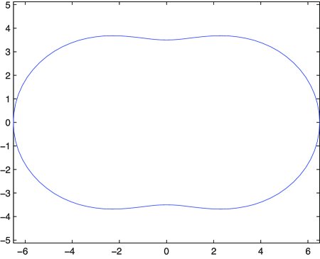
Figure 6: The non-convex curve considered in example 6.2.

Again, the simulation results for the closed-loop system with controller (19) and $K_{1}=5$, $K_{2}=2$ are shown in Figures 7, 8 for the initial condition $(\varphi(0),\dot{\varphi}(0),s(0),\dot{s}(0))=(0,0,0,2)$.

\psfrag{t}{$t$}\psfrag{P}{$\Phi(s(t))$}\psfrag{Q}{$\varphi(t)$}\includegraphics[width=234.87749pt]{FIGURES/non_convex_closed_loop2bis}

Figure 7: Simulation of the closed-loop system for the curve considered in example 6.2. The solution converges to the constraint manifold $\Gamma$.

\psfrag{s}{$s$}\psfrag{t}{$\dot{s}$}\psfrag{R}{$\mathcal{R}$}\includegraphics[width=234.87749pt]{FIGURES/non_convex_closed_loop1bis}

Figure 8: Simulation of the closed-loop system for the curve considered in example 6.2. The solution converges to the submanifold $\mathcal{R}\subset\Gamma$.

References

• [1] N. Getz, Control of balance for a nonlinear nonholonomic non- minimum phase model of a bicycle, in: American Control Conference, 1994, pp. 148–151.
• [2] N. Getz, J. Marsden, Control for an autonomous bicycle, in: IEEE International Conference on Robotics and Automation, Vol. 2, 1995, pp. 1397–1402 vol.2.
• [3] J. Hauser, A. Saccon, R. Frezza, Achievable motorcycle trajectories, in: IEEE Conference on Decision and Control, 2004.
• [4] J. Hauser, A. Saccon, Motorcycle modeling for high-performance maneuvering, IEEE Control Systems Magazine (2006) 89–105.
• [5] J. Hauser, S. Sastry, G. Meyer, Nonlinear control design for slightly non-minimum phase systems: Applications to V/STOL aircraft, Automatica 28 (4) (1992) 665–679.
• [6] L. Consolini, M. Maggiore, C. Nielsen, M. Tosques, Path following for the pvtol aircraft, Automatica 46 (8) (2010) 1284–1296.
• [7] F. Plestan, J. Grizzle, E. Westervelt, G. Abba, Stable walking of a 7-DOF biped robot, IEEE Transactions on Robotics and Automation 19 (4) (2003) 653–668.
• [8] E. Westervelt, J. Grizzle, D. Koditschek, Hybrid zero dynamics of planar biped robots, IEEE Transactions on Automatic Control 48 (1) (2003) 42–56.
• [9] C. Canudas-de-Wit, On the concept of virtual constraints as a tool for walking robot control and balancing, Annual Reviews in Control 28 (2004) 157–166.
• [10] A. Shiriaev, J. Perram, C. Canudas-de-Wit, Constructive tool for orbital stabilization of underactuated nonlinear systems: Virtual constraints approach, IEEE Transactions on Automatic Control 50 (8) (2005) 1164–1176.
• [11] L. Freidovich, A. Robertsson, A. Shiriaev, R. Johansson, Periodic motions of the Pendubot via virtual holonomic constraints: Theory and experiments, Automatica 44 (2008) 785–791.
• [12] A. M. Bloch, Nonholonomic Mechanics and Control, Interdisciplinary Applied Mathematics: Systems and Control, Springer-Verlag, New York, 2003.
• [13] A. Shiriaev, L. Freidovich, S. Gusev, Transverse linearization for controlled mechanical systems with several passive degrees of freedom, IEEE Transactions on Automatic Control 55 (4) (2010) 893–906.
• [14] A. Shiriaev, L. Freidovich, A. Robertsson, R. Johansson, A. Sandberg, Virtual-holonomic-constraints-based design of stable oscillations of Furuta pendulum: Theory and experiments, IEEE Transactions on Robotics 23 (4) (2007) 827–832.
• [15] M. Maggiore, L. Consolini, Virtual holonomic constraints for Euler-Lagrange systems, IEEE Transactions on Automatic Control 58 (4) (2013) 1001–1008.
• [16] J. Lee, Introduction to Smooth Manifolds, 2nd Edition, Springer, 2013.
• [17] L. Consolini, M. Maggiore, Virtual holonomic constraints for Euler-Lagrange systems, in: Proceedings of the 8th IFAC Symposium on Nonlinear Control Systems (NOLCOS), Bologna, Italy, 2010.
• [18] H. K. Khalil, Nonlinear Systems, 3rd Edition, Prentice Hall, 2002.
• [19] A. Shiriaev, A. Robertsson, J. Perram, A. Sandberg, Periodic motion planning for virtually constrained Euler-Lagrange systems, Systems and Control Letters 55 (11) (2006) 900 – 907.
• [20] P. Hartman, Ordinary differential equations, 2nd Edition, SIAM Classics in Applied Mathematics, 2002.
• [21] A. Mohammadi, M. Maggiore, L. Consolini, When is a Lagrangian control system with virtual holonomic constraints Lagrangian?, in: Proceedings of the 9th IFAC Symposium on Nonlinear Control System, Toulouse, France, 2013.
• [22] A. Polyanin, V. Zaitsev, Handbook of exact solutions for ordinary differential equations, CRC press, 2003.
• [23] P. Seibert, J. S. Florio, On the reduction to a subspace of stability properties of systems in metric spaces, Annali di Matematica pura ed applicata CLXIX (1995) 291–320.
• [24] M. El-Hawwary, M. Maggiore, Reduction theorems for stability of closed sets with application to backstepping control design, Automatica 49 (1) (2012) 214–222.