From rough path estimates to multilevel Monte Carlo

Abstract.

New classes of stochastic differential equations can now be studied using rough path theory (e.g. Lyons et al. [LCL07] or Friz–Hairer [FH14]). In this paper we investigate, from a numerical analysis point of view, stochastic differential equations driven by Gaussian noise in the aforementioned sense. Our focus lies on numerical implementations, and more specifically on the saving possible via multilevel methods. Our analysis relies on a subtle combination of pathwise estimates, Gaussian concentration, and multilevel ideas. Numerical examples are given which both illustrate and confirm our findings.

1. Introduction

We consider implementable schemes for large classes of stochastic differential equations (SDEs)

(1) $$dY_{t}=V_{0}\left(Y_{t}\right)dt+\sum_{i=1}^{d}V_{i}\left(Y_{t}\right)\,dX_{t}^{i}\left(\omega\right)$$

driven by multidimensional Gaussian signals, say $X=X_{t}\left(\omega\right)\in\mathbb{R}^{d}.$ The interpretation of these equations is in Lyons’ rough path sense [LQ02, LCL07, FV10b, FH14]. In essence, one deals with generalizations of classical Stratonovich SDE meaning for such equations. One requires some smoothness/boundedness conditions on the vector fields $V_{0}$ and $V\equiv\left(V_{1},\dots,V_{d}\right)$; for the sake of this introduction, the reader may assume bounded vector fields with bounded derivatives of all order (but we will be more specific later). This also requires a “natural” lift of $X\left(\cdot,\omega\right)$ to a (random) rough path

(2) $$\mathbf{X}_{t}\left(\omega\right)=\sum_{i=1}^{N}\int_{0<s_{1}<\cdots<s_{i}<t}dX_{s_{1}}(\omega)\otimes\cdots\otimes dX_{s_{i}}(\omega),$$

see, e.g., [LCL07, Ch. 3]. In (2), $N$ is related to the roughness of $X$. For instance, in the case of Brownian motion, we need $N=2$, but rougher processes $X$ require $N>2$. The reader not familiar with rough path theory may think of $Y$ as “Stratonovich” solution to (1). In fact, $Y$ is known to be the Wong-Zakai limit, obtained by replacing $X$ in (1) by piecewise-linear approximation followed by taking the mesh-to-zero limit.

We shall simplify the discussion by choosing $V_{0}\equiv 0$ and using the short-hand notation

(3) $$dY_{t}=V\left(Y_{t}\right)d\mathbf{X}_{t},$$

indicating that the differential equation is driven by the rough path $\mathbf{X}$ given in (2). Of course, it would be easy to include equations of the form (1) into the framework (3), e.g., by including time $t$ as an additional (smooth) component of the noise $X$. This setting includes, for instance, fractional Brownian motion (fBm) with Hurst parameter $H>1/4$, see [CQ02]. It may help the reader to recall that, in the case when $X=B$, a multidimensional Brownian motion, all this amounts to enhance $B$ with Lévy’s stochastic area or, equivalently, with all iterated stochastic integrals of $B$ against itself, say $\mathbb{B}_{s,t}=\int_{s}^{t}B_{s,u}\otimes dB_{u}$. The (rough-)pathwise solution concept then agrees with the usual notion of an SDE solution (in Itô- or Stratonovich sense, depending on which integration was used in defining $\mathbb{B}$). As is well-known this provides a robust extension of the usual Itô framework of stochastic differential equations with an exploding number of new applications (including non-linear SPDE theory, robustness of the filtering problem, non-Markovian Hörmander theory).

Gaussian noise more general than Brownian motion is also interesting from a modelling point of view. Many stochastic models are based on independent identically distributed noise terms, which lead to dynamics driven by standard Brownian motion (or similar Lévy processes) under re-scaling. Arguably, this choice is often based on convenience, since the resulting Markovian models are fairly simple to analyze. Besides, quantities of interest in Markovian models are often relatively easy to compute, with different numerical techniques available. On the other hand, non-trivial correlations in the noise can lead to more general (Gaussian) processes (under re-scaling) such as fractional Brownian motion. These models are typically much more difficult to both analyze and compute, but may well be adequate to explain features of the underlying real world phenomena. For instance, some recent studies in finance report excellent fits of (simple) asset price models driven by fractional Brownian motions to market data, substantially improving the performance of models (even more complex ones) driven by standard Brownian motion. We refer to [GJR14a, BFG15] for more information. The importance of fractional Brownian motion for models of turbulence has been understood since the 1940s, see, for instance, [SS94]. Rough path analysis provides a framework for analysis and numerics for these kind of models.

In a sense, the rough path interpretation of a differential equation is closely related to strong, pathwise error estimates of Euler- resp. Milstein-approximation to stochastic differential equations. For instance, Davie’s definition [Dav07] of a (rough)pathwise SDE solution is

(4) $$Y_{t}-Y_{s}\equiv Y_{s,t}=V_{i}\left(Y_{s}\right)B_{s,t}^{i}+V_{i}^{k}\left(Y_{s}\right)\partial_{k}V_{j}\left(Y_{s}\right)\mathbb{B}_{s,t}^{i,j}+o\left(\left|t-s\right|\right)\text{ as }t-s\downarrow 0,$$

where we employ Einstein’s convention. In fact, this becomes an entirely deterministic definition, only assuming

$$\exists\alpha\in\left(1/3,1/2\right):\left|B_{s,t}\right|\leq C\left|t-s\right|^{\alpha},\left|\mathbb{B}_{s,t}\right|\leq C\left|t-s\right|^{2\alpha},\text{ \ \ }$$

something which is known to hold true almost surely (i.e. for $C=C\left(\omega\right)<\infty$ a.s.), and something which is not at all restricted to Brownian motion. As the reader may suspect this approach leads to almost-sure convergence (with rates) of schemes which are based on the iteration of the approximation seen in the right-hand-side of (4). The practical trouble is that Lévy’s area, the anti-symmetric part of $\mathbb{B}$, is notoriously difficult to simulate; leave alone the simulation of Lévy’s area for other Gaussian processes. It has been understood for a while, at least in the Brownian setting, that the truncated (or: simplified) Milstein scheme, in which Lévy’s area is omitted, i.e. replace $\mathbb{B}_{s,t}$ by $Sym\left(\mathbb{B}_{s,t}\right)$ in (4), still offers benefits: For instance, Talay [Tal86] replaces Lévy area by suitable Bernoulli r.v. such as to obtain weak order $1$ (see also Kloeden–Platen [KP92] and the references therein). In the multilevel context, [GS14] use this truncated Milstein scheme together with a sophisticated antithetic (variance reduction) method. Finally, in the rough path context this scheme was used in [DNT12]: the convergence of the scheme can be traced down to an underlying Wong-Zakai type approximation for the driving random rough path – a (probabilistic!) result which is known to hold in great generality for stochastic processes, starting with [CQ02] in the context of fractional Brownian motion, see [FV10b, Ch. 15] and the references therein.

A rather difficult problem is to go from almost-sure convergence (with rates) to $L^{1}$ (or ever: $L^{r}$ any $r<\infty$) convergence. Indeed, as pointed out in [DNT12, Remark 1.2]: ”Note that the almost sure estimate [for the simplified Milstein scheme] cannot be turned into an $L^{1}$-estimate […]. This is a consequence of the use of the rough path method, which exhibits non-integrable (random) constants.” The resolution of this problem forms the first contribution of this paper. It is based on some recent progress [CLL13], see also [FR13], initially developed to prove smoothness of laws for (non-Markovian) SDEs driven by Gaussian signals under a Hörmander condition, [CF10, HP13].

Having established $L^{r}$-convergence (any $r<\infty$, with rates) for implementable “simplified” Milstein schemes we move to the second contribution of the paper: a multilevel algorithm, in the sense of Giles [Gil08b], for stochastic differential equations driven by large classes of Gaussian signals.

The savings here are rather dramatic. In absence of Markovian structure, the strong rate must proxy for the weak rate, which leaves one with complexity $\mathcal{O}(\epsilon^{-\theta-2})$, any $\theta>2\rho/(2-\rho)$ where the parameter $\rho$ quantifies the roughness of the noise. With multilevel, we reduce this to $\mathcal{O}(\epsilon^{-\theta})$. For instance, in the case of fBm with $H=0.4$, one has $\rho=1.25$ and thus $\theta\sim 3.33$, which is only marginally worse than single level Monte Carlo in the Brownian motion context (where one has $\theta=3$). On the other hand, the computational cost of single-level Monte Carlo would be proportional to $\varepsilon^{-\theta-2}\sim\varepsilon^{-5.33}$ which corresponds to a numerically non-feasible situation.

A strong, $L^{2}$ error estimate (“rate $\beta/2$”) is the key assumption in Giles’ complexity theorem, and this is precisely what we have established in the first part. Some other extension of the Giles theorem are necessary; indeed it is crucial to allow for a weak rate of convergence $\alpha<1/2$ (ruled out explicitly in [Gil08b]) whenever we deal with driving signals with sample path regularity “worse” then Brownian motion. We are able to do all this, moreover we carefully keep track of the relevant constants in front of the asymptotic terms, a necessity in such an irregular regime.

Let us now discuss the algorithm in more detail. We consider the following scheme for approximating $Y$, see [DNT12, FV10b]. Given an equi-distant dissection $D=\left(t_{k}\right)$ of $\left[0,T\right]$ with mesh $h$, so that $t_{k+1}-t_{k}\equiv h$ for all $k$, write $X_{t_{k},t_{k+1}}$ for the corresponding increments. We then define $\overline{Y}_{0}\equiv Y_{0}$ and the “simplified” step-$3$ Euler scheme

(5) $$\overline{Y}_{t_{k+1}}=\overline{Y}_{t_{k}}+\sum_{l=1}^{3}\frac{1}{l!}V_{i_{1}}\cdots V_{i_{l}}I\left(\overline{Y}_{t_{k}}\right)X_{t_{k},t_{k+1}}^{i_{1}}\cdots X_{t_{k},t_{k+1}}^{i_{l}},$$

where $I(y)=y$ is the identity function and the vector fields $V_{1},\ldots,V_{d}$, unless otherwise stated assumed bounded with bounded derivatives of all orders, are viewed as linear first order operators. Whenever convenient we extend $\overline{Y}$ to $\left[0,T\right]$ by linear interpolation. Moreover, the Einstein summation convention is in force. For a more detailed description of the algorithm we refer to Section 3.3. We are now able to state (a simple version of) our main results; cf. Corollary 17:

Theorem 1 (Strong rates).

Let $X=\left(X^{1},\dots,X^{d}\right)$ be a continuous, zero-mean Gaussian process with independent components. Assume furthermore that each component has stationary increments and that

$$\sigma^{2}\left(t-s\right):=E\left|X_{t}^{i}-X_{s}^{i}\right|^{2}$$

where $\sigma^{2}$ is concave and $\sigma^{2}\left(\tau\right)=\mathcal{O}\left(\tau^{1/\rho}\right)$ as $\tau\rightarrow 0$ for some $\rho\in[1,2).$
Let $Y$ be the solution to the rough differential equation (3) driven by (the rough path lift) of $X$ and $\overline{Y}=\overline{Y}^{h}$ be the approximate solution based on (5). Then we have strong convergence of (almost) rate $1/\rho-1/2$. More precisely, for any $1\leq r<\infty$ and $\delta>0$, there exists a constant $C$ such that

$$\left|E\left(\sup_{t\in\left[0,T\right]}\left|Y_{t}-\overline{Y}_{t}^{h}\right|^{r}\right)\right|^{\frac{1}{r}}\leq Ch^{1/\rho-1/2-\delta}.$$

The reader should notice that the assumption on $X$ is met by multidimensional Brownian motion (with $\rho=1$) in which case $Y$ is nothing but a Stratonovich solution of the SDE (1), which of course may be rewritten as Itô equation. More interestingly, $X$ may be a fractional Brownian motion (with $\rho=\frac{1}{2H}>1$) in the (interesting) “rougher than Brownian” regime $H\in(1/4,1/2)$. However, stationarity of increments of $X$ plays very little role aside from allowing an easy-to-state formulation above. The precise technical requirement is given in Condition 10 below and is satisfied in many examples, see [FGGR16].

Using Giles’ multi-level Monte Carlo methodology, we can greatly improve the complexity bounds for the discretization algorithm (5), see Theorem 23. Note that the overall computational cost depends on the computational cost of simulating the increments of the process $X$ as needed in equation (5). For each trajectory of $Y$, we need to sample a vector of increments of $X$ of length $N\equiv T/h$, i.e., we need to sample from an $N$-dimensional normal distribution with known non-diagonal covariance matrix. In general, this can be achieved at cost proportional to $N^{2}$ by multiplication of a standard normal vector with the lower triangular factor obtained by the Cholesky factorization of the covariance matrix. In many special cases, for instance for fBm, the cost can be reduced to $N\log N$, see [Die04], and we concentrate on this scenario below. The precise statement is given in Theorem 23.

Theorem 2 (Multilevel complexity estimate).

Let $X$ and $Y$ be as in the previous theorem and $f:C([0,T],\mathbb{R}^{m})\rightarrow\mathbb{R}^{n}$ a Lipschitz continuous functional. Assume that the computational cost of generating a vector of (non-overlapping) increments of $X$ of length $N$ is proportional to $N\log N$. Then the Monte Carlo evaluation of a path-dependent functional of the form

$$E(f(Y_{t}:0\leq t\leq T))$$

to within a MSE of $\varepsilon^{2}$, can be achieved with computational work

$$\mathcal{O}\left(\varepsilon^{-\theta}\right),\quad\forall\theta>\frac{2\rho}{2-\rho}.$$

As a sanity check, let us compare this results with the corresponding, well-known results for classical stochastic differential equations (here: in Stratonovich sense) driven by $d$-dimensional Brownian motion $B$. The assumptions on $X$ are clearly met with $\rho=1$. As a consequence, we obtain strong convergence of (almost) rate $1/2$ in agreement with the well-known strong rate $1/2$ in the classical setting. Concerning our multilevel complexity estimate, we obtain (almost) order $\varepsilon^{-2}$ which is arbitrarily ”close” to known result $\mathcal{O}\left(\varepsilon^{-2}\left(\log\varepsilon\right)^{2}\right)$ [Gil08a, Gil08b], recently sharpened to $\mathcal{O}\left(\varepsilon^{-2}\right)$ [GS14] with the aid of a suitable antithetic multilevel correction estimator.

Let us summarize the (computational) benefits of the multilevel approach in the present (“rougher than Brownian”) setting. A direct Monte Carlo implementation of the scheme (5) would require a complexity of $\mathcal{O}(\varepsilon^{-(2+1/\alpha)})$ in order to attain an MSE of no more than $\varepsilon^{2}$. Here, $\alpha$ is the weak rate of convergence of the scheme. On the other hand, we show in Theorem 18 that the complexity is only $\mathcal{O}(\varepsilon^{-(1+2\alpha-\beta)/\alpha})$ for the multi-level Monte Carlo estimator, where $\beta$ is two times the strong rate of convergence. Thus, when the weak rate of convergence is equal to the strong rate of convergence, then the complexity of the multi-level estimator is reduced by a factor $\varepsilon^{2}$ as compared by the complexity of the standard Monte Carlo estimator. When the weak rate is two times the strong rate, the speed up is still by a factor $\varepsilon$, see Table 1 and Table 2.

2. Rough path estimates revisited

In this section, we revisit some classical estimates used in rough paths theory. Definitions of the basic objects and all relevant notation may be found in the appendix. A more detailed account to the theory of rough paths may be found in the monographs [LQ02], [LCL07], [FV10b] or [FH14].

Versions of the results we are interested in (cf. the forthcoming theorems 4 and 8) are already stated in the above mentioned references, and the given estimates are (essentially) sharp when the oscillations of the driving rough path (i.e. its $p$-variation) become small. However, it turns out that they are less useful when its oscillations get large. In this case, we will show that the estimates can be improved by replacing the occurring $p$-variation norm of the rough path $\mathbf{x}$ in the inequality by another quantity $N(\mathbf{x})$ which was first introduced by Cass-Litterer-Lyons in [CLL13] (and which we recall in Definition 3 below). This becomes crucial when substituting the deterministic rough path $\mathbf{x}$ by the lift of a Gaussian process $\mathbf{X}$: A key result in [CLL13] states that the quantity $N(\mathbf{X})$ enjoys significantly better integrability properties than the $p$-variation of $\mathbf{X}$.

The aim of this section is to show that one can indeed improve the bound for the Lipschitz constant of the Itô-Lyons map (Theorem 4) and the estimate for the distance of the solution of a rough differential equation (RDE) and its Euler (or Milstein) approximation (Theorem 8). This will allow us to deduce the desired probabilistic estimates in the forthcoming section 3.

2.1. Improved bounds for the Lipschitz constant of the Itô-Lyons map

Recall the following definition, taken from [CLL13]:

Definition 3.

Let $\omega$ be a control function, that is, a continuous function $\omega\colon\{(s,t)\,:\,0\leq s\leq t\leq T\}\to[0,\infty)$ for which $\omega(s,t)+\omega(t,u)\leq\omega(s,u)$ holds for every $s\leq t\leq u$. For $\alpha>0$ and $\left[s,t\right]\subset\left[0,T\right]$, we set

$$\tau_{0}\left(\alpha\right) = s$$

$$\tau_{i+1}\left(\alpha\right) = \inf\left\{u:\omega\left(\tau_{i}(\alpha),u\right)\geq\alpha,\tau_{i}\left(\alpha\right)<u\leq t\right\}\wedge t$$

and define

$$N_{\alpha,\left[s,t\right]}\left(\omega\right)=\sup\left\{n\in\mathbb{N\cup}\left\{0\right\}:\tau_{n}\left(\alpha\right)<t\right\}.$$

When $\omega$ arises from the (homogenous) $p$-variation norm $\|\cdot\|_{p-\text{var}}$ of a ($p$-rough) path, $\mathbf{x}$, i.e. $\omega_{\mathbf{x}}=\left\|\mathbf{x}\right\|_{p\text{-var;}\left[\cdot,\cdot\right]}^{p}$ with $p\geq 1$, we shall also write $N_{\alpha,\left[s,t\right]}\left(\mathbf{x}\right):=N_{\alpha,\left[s,t\right]}\left(\omega_{\mathbf{x}}\right)$.

It is easy to see that $\alpha N_{\alpha,[0,T]}\left(\mathbf{x}\right)\leq\|\mathbf{x}\|_{p-\text{var};[0,T]}^{p}$ ([CLL13, Lemma 4.9]), and this is sharp (as one can see choosing $\alpha\nearrow\|\mathbf{x}\|_{p-\text{var};[0,T]}^{p}$). However, for fixed $\alpha$, the tail estimates for $N_{\alpha,[0,T]}\left(\mathbf{X}\right)$ are significantly better than for $\|\mathbf{X}\|_{p-\text{var};[0,T]}^{p}$ when we consider Gaussian lifts $\mathbf{X}$, cf. [CLL13] and [FR13].

Next, we give the main result of this section. The following theorem is a variant of [FV10b, Theorem 10.38]. The main difference is that in [FV10b, Theorem 10.38], the Lipschitz constant is (essentially) given by $C\exp\left\{C\left(\|\mathbf{x}^{1}\|_{p-\text{var};[0,T]}^{p}+\|\mathbf{x}^{2}\|_{p-\text{var};[0,T]}^{p}\right)\right\}$, whereas in the following theorem, $\|\mathbf{x}^{i}\|_{p-\text{var};[0,T]}^{p}$ is replaced by $N_{\alpha,[0,T]}(\mathbf{x}^{i})$, $i=1,2$.

Theorem 4.

Consider the RDEs

$$dy_{t}^{i}=V^{i}(y_{t}^{i})\,d\mathbf{x}_{t}^{i};\quad y_{0}^{i}\in\mathbb{R}^{e}$$

for $i=1,2$ on $[0,T]$ where $V^{1}$ and $V^{2}$ are two families of vector fields, $\gamma>p$ and $\nu$ is a bound on $|V^{1}|_{Lip^{\gamma}}$ and $|V^{2}|_{Lip^{\gamma}}$. Then for every $\alpha>0$ there is a constant $C=C(\gamma,p,\nu,\alpha)$ such that

$$\left|y^{1}-y^{2}\right|_{\infty\text{;}\left[0,T\right]} \leq \ C\left[|y_{0}^{1}-y_{0}^{2}|+\left|V^{1}-V^{2}\right|_{\text{Lip}^{\gamma-1}}+\rho_{p-\text{var};[0,T]}(\mathbf{x}^{1},\mathbf{x}^{2})\right]$$

$$\times\exp\left\{C\left(N_{\alpha,[0,T]}(\mathbf{x}^{1})+N_{\alpha,[0,T]}(\mathbf{x}^{2})\right)\right\}$$

holds.

The proof of Theorem 4 will be given at the end of this section. We first prove some preparatory lemmata. Recall that if $\omega^{1}$ and $\omega^{2}$ are controls, also $\omega^{1}+\omega^{2}$ is a control.

Lemma 5.

Let $\omega^{1}$ and $\omega^{2}$ be two controls. Then

$$N_{\alpha,[s,t]}(\omega^{1}+\omega^{2})\leq 2N_{\alpha,[s,t]}(\omega^{1})+2N_{\alpha,[s,t]}(\omega^{2})+2$$

for every $s<t$ and $\alpha>0$.

Proof.

If $\omega$ is any control, set

$$\omega_{\alpha}\left(s,t\right):=\sup\left\{\sum_{i=0}^{M-1}\omega(t_{i},t_{i+1})\,:\,s=t_{0}<t_{1}<\ldots<t_{M}=t,\ \omega(t_{i},t_{i+1})\leq\alpha,\ n\in\mathbb{N}\right\}.$$

If $\bar{\omega}:=\omega^{1}+\omega^{2}$, $\bar{\omega}(t_{i},t_{i+1})\leq\alpha$ implies $\omega^{i}(t_{i},t_{i+1})\leq\alpha$ for $i=1,2$ and therefore $\bar{\omega}_{\alpha}\left(s,t\right)\leq\omega_{\alpha}^{1}\left(s,t\right)+\omega_{\alpha}^{2}\left(s,t\right)$. From Proposition 4.6 in [CLL13] we know that $\omega_{\alpha}^{i}\left(s,t\right)\leq\alpha\left(2N_{\alpha,\left[s,t\right]}\left(\omega^{i}\right)+1\right)$ for $i=1,2$. We conclude

$$\alpha N_{\alpha,\left[s,t\right]}\left(\bar{\omega}\right) =\sum_{i=0}^{N_{\alpha,\left[s,t\right]}\left(\bar{\omega}\right)-1}\bar{\omega}(\tau_{i}\left(\alpha\right),\tau_{i+1}\left(\alpha\right))\leq\bar{\omega}_{\alpha}(s,t)\leq\omega_{\alpha}^{1}\left(s,t\right)+\omega_{\alpha}^{2}\left(s,t\right)$$

$$\leq\alpha\left(2N_{\alpha,\left[s,t\right]}\left(\omega^{1}\right)+2N_{\alpha,\left[s,t\right]}\left(\omega^{2}\right)+2\right).$$

∎

Lemma 6.

Let $\omega^{1}$ and $\omega^{2}$ be two controls and assume that $\omega^{2}(s,t)\leq K$. Then

$$N_{\alpha,[s,t]}(\omega^{1}+\omega^{2})\leq N_{\alpha-K,[s,t]}(\omega^{1})$$

for every $\alpha>K$.

Proof.

Set $\bar{\omega}:=\omega^{1}+\omega^{2}$ and

$$\bar{\tau}_{0}\left(\alpha\right) = s$$

$$\bar{\tau}_{i+1}\left(\alpha\right) = \inf\left\{u:\bar{\omega}\left(\bar{\tau}_{i}(\alpha),u\right)\geq\alpha,\bar{\tau}_{i}\left(\alpha\right)<u\leq t\right\}\wedge t.$$

Similarly, we define $(\tau_{i})_{i\in\mathbb{N}}=(\tau_{i}(\alpha-K))_{i\in\mathbb{N}}$ for $\omega^{1}$. It suffices to show that $\bar{\tau}_{i}\geq\tau_{i}$ for $i=0,\ldots,N_{\alpha,[s,t]}(\bar{\omega})$. We do this by induction. For $i=0$, this is clear. If $\bar{\tau}_{i}\geq\tau_{i}$ for some $i\leq N_{\alpha,[s,t]}(\bar{\omega})-1$, superadditivity of control functions gives

$$\alpha=\bar{\omega}(\bar{\tau}_{i},\bar{\tau}_{i+1})\leq\omega^{1}(\tau_{i},\bar{\tau}_{i+1})+K$$

which implies $\tau_{i+1}\leq\bar{\tau}_{i+1}$. ∎

For the next Lemma, recall the definition of the homogenous $p$-$\omega$ distance and -norm given in the appendix and in [FV10b, Definition 8.2].

Lemma 7.

Let $s<t\in[0,T]$ and assume that $\|\mathbf{x}^{i}\|_{p-\omega;[s,t]}\leq 1$ for $i=1,2$. Then there is a constant $C=C(\gamma,p)$ such that

$$\nu|y^{1}-y^{2}|_{\infty;[s,t]}\leq \left[\nu|y_{s}^{1}-y_{s}^{2}|+\left|V^{1}-V^{2}\right|_{\text{Lip}^{\gamma-1}}+\nu\rho_{p-\omega;[s,t]}(\mathbf{x}^{1},\mathbf{x}^{2})\right]$$

$$\times(N_{\alpha,[s,t]}(\omega)+1)\exp\left\{C\nu^{p}\alpha(N_{\alpha,[s,t]}(\omega)+1)\right\}$$

for every $\alpha>0$.

Proof.

Set $\bar{y}=y^{1}-y^{2}$ and

$$\kappa=\frac{\left|V^{1}-V^{2}\right|_{\text{Lip}^{\gamma-1}}}{\nu}+\rho_{p-\omega;[s,t]}(\mathbf{x}^{1},\mathbf{x}^{2}).$$

From [FV10b, Theorem 10.26] we can deduce that there is a constant $C=C(\gamma,p)$ such that

$$|\bar{y}_{u,v}|\leq C\nu\omega(u,v)^{1/p}\left[|\bar{y}_{u}|+\kappa\right]\exp\left\{C\nu^{p}\omega(u,v)\right\}$$

for every $u<v\in[s,t]$. From $|\bar{y}_{u,v}|\geq|\bar{y}_{s,v}|-|\bar{y}_{s,u}|$ we obtain

$$|\bar{y}_{s,v}| \leq C\nu\omega(u,v)^{1/p}\left[|\bar{y}_{u}|+\kappa\right]\exp\left\{C\nu^{p}\omega(u,v)\right\}+|\bar{y}_{s,u}|$$

$$\leq\left[|\bar{y}_{s}|+|\bar{y}_{s,u}|+\kappa\right]\exp\left\{C\nu^{p}\omega(u,v)\right\}$$

for $s\leq u<v\leq t$. Now let $s=\tau_{0}<\tau_{1}<\ldots<\tau_{M}<\tau_{M+1}=v\leq t$ for $M\geq 0$. By induction, one sees that

$$|\bar{y}_{s,v}| \leq(M+1)(|\bar{y}_{s}|+\kappa)\exp\left\{C\nu^{p}\sum_{i=0}^{M}\omega(\tau_{i},\tau_{i+1})\right\}$$

$$\leq C^{M+1}\left[|\bar{y}_{s}|+\kappa\right]\exp\left\{C\nu^{p}\sum_{i=0}^{M}\omega(\tau_{i},\tau_{i+1})\right\}.$$

It follows that for every $v\in[s,t]$,

$$|\bar{y}_{s,v}|\leq\left[|\bar{y}_{s}|+\kappa\right](N_{\alpha,[s,t]}(\omega)+1)\exp\left\{C\nu^{p}\alpha(N_{\alpha,[s,t]}(\omega)+1)\right\},$$

therefore

$$|\bar{y}_{v}|\leq\left[|\bar{y}_{s}|+\kappa\right](N_{\alpha,[s,t]}(\omega)+1)\exp\left\{C\nu^{p}\alpha(N_{\alpha,[s,t]}(\omega)+1)\right\}+|\bar{y}_{s}|$$

and finally

$$|\bar{y}|_{\infty;[s,t]}\leq\left[|\bar{y}_{s}|+\kappa\right](N_{\alpha,[s,t]}(\omega)+1)\exp\left\{C\nu^{p}\alpha(N_{\alpha,[s,t]}(\omega)+1)\right\}.$$

∎

Proof of Theorem 4.

Let $\omega$ be a control such that $\|\mathbf{x}^{i}\|_{p-\omega;[0,T]}\leq 1$ for $i=1,2$ (the precise choice of $\omega$ will be made later). From Lemma 7 we know that there is a constant $C=C(\gamma,p,\nu,\alpha)$ such that

$$\left|y^{1}-y^{2}\right|_{\infty\text{;}\left[0,T\right]} \leq\left[|y_{0}^{1}-y_{0}^{2}|+\left|V^{1}-V^{2}\right|_{\text{Lip}^{\gamma-1}}+\rho_{p-\omega;[s,t]}(\mathbf{x}^{1},\mathbf{x}^{2})\right]$$

$$\times\exp\left\{C(N_{\alpha,[s,t]}(\omega)+1)\right\}.$$

Now we set $\omega=\omega_{\mathbf{x}^{1},\mathbf{x}^{2}}$ where

$$\omega_{\mathbf{x}^{1},\mathbf{x}^{2}}(s,t)=\|\mathbf{x}^{1}\|_{p-\text{var};[s,t]}^{p}+\|\mathbf{x}^{2}\|_{p-\text{var};[s,t]}^{p}+\sum_{k=1}^{\lfloor p\rfloor}\frac{\left(\rho_{p-\text{var};[s,t]}^{(k)}(\mathbf{x}^{1},\mathbf{x}^{2})\right)^{p/k}}{\left(\rho_{p-\text{var};[0,T]}^{(k)}(\mathbf{x}^{1},\mathbf{x}^{2})\right)^{p/k}}$$

(the definition of $\rho_{p-\text{var}}^{(k)}(\cdot,\cdot)$ may be found in the appendix). It is easy to check that

$$\|\mathbf{x}^{1}\|_{p-\omega_{\mathbf{x}^{1},\mathbf{x}^{2}};[0,T]} \leq 1,\quad\|\mathbf{x}^{2}\|_{p-\omega_{\mathbf{x}^{1},\mathbf{x}^{2}};[0,T]}\leq 1\quad\text{ and}$$

$$\rho_{p-\omega_{\mathbf{x}^{1},\mathbf{x}^{2}};[0,T]}(\mathbf{x}^{1},\mathbf{x}^{2}) \leq\rho_{p-\text{var};[0,T]}(\mathbf{x}^{1},\mathbf{x}^{2}).$$

Finally, if $\alpha>\lfloor p\rfloor$ we can use Lemma 6 and Lemma 5 to see that

$$N_{\alpha,[0,T]}(\omega_{\mathbf{x}^{1},\mathbf{x}^{2}})+1 \leq N_{\alpha-\lfloor p\rfloor,[0,T]}(\omega_{\mathbf{x}^{1}}+\omega_{\mathbf{x}^{2}})+1$$

$$\leq 3\left(N_{\alpha-\lfloor p\rfloor,[0,T]}(\mathbf{x}^{1})+N_{\alpha-\lfloor p\rfloor,[0,T]}(\mathbf{x}^{2})+1\right).$$

Substituting $\alpha\mapsto\alpha+\lfloor p\rfloor$ gives the claimed estimate. ∎

2.2. Improved bounds for the higher order Euler approximations

We are now interested in proving a similar estimate for the distance between Euler-/Milstein approximations for rough paths and the actual solution (for the purpose of unified terminology, in the sequel we will only speak of Euler-schemes). Recall the notation from [FV10b]: If $V=\left(V_{1},\ldots,V_{d}\right)$ is a collection of sufficiently smooth vector fields on $\mathbb{R}^{e}$, $g\in T^{N}\left(\mathbb{R}^{d}\right)$ and $y\in\mathbb{R}^{e}$, we define an increment of the step-$N$ Euler scheme by

$$\mathcal{E}_{\left(V\right)}\left(y,g\right):=\sum_{k=1}^{N}V_{i_{1}}\ldots V_{i_{k}}I\left(y\right)g^{k,i_{1},\ldots,i_{k}}$$

where $g^{k,i_{1},\ldots,i_{k}}=\pi_{k}\left(g\right)^{i_{1},\ldots,i_{k}}\in\mathbb{R}$, $I$ is the identity on $\mathbb{R}^{e}$ and every $V_{j}$ is identified with the first-order differential operator $V_{j}^{k}\left(y\right)\frac{\partial}{\partial y^{k}}$ (throughout, we use the Einstein summation convention). Furthermore, we set

$$\mathfrak{E}^{g}y:=y+\mathcal{E}_{\left(V\right)}\left(y,g\right).$$

Given $D=\left\{0=t_{0}<\ldots<t_{n}=T\right\}$ and a path $\mathbf{x}\in C^{p-var}_{0}\left(\left[0,T\right];G^{\lfloor p\rfloor}\left(\mathbb{R}^{d}\right)\right)$ we define the (step-$N$) Euler approximation to the RDE solution $y$ of

(6) $$dy=V(y)\,d\mathbf{x}$$

with starting point $y_{0}\in\mathbb{R}^{e}$ at time $t_{k}\in D$ by

$$y_{t_{k}}^{\text{Euler;}D}:=\mathfrak{E}^{t_{k}\leftarrow t_{0}}y_{0}:=\mathfrak{E}^{S_{N}\left(\mathbf{x}\right)_{t_{k-1},t_{k}}}\circ\cdots\circ\mathfrak{E}^{S_{N}\left(\mathbf{x}\right)_{t_{0},t_{1}}}y_{0}$$

where $S_{N}\left(\mathbf{x}\right)$ denotes the Lyons lift of the rough path $\mathbf{x}$, see [FV10b, Section 9.1].

The following theorem is a version of [FV10b, Theorem 10.30] where, as in Theorem 4, the estimate is improved by replacing the quantity $\|\cdot\|_{p-\text{var};[0,T]}^{p}$ by $N_{\alpha,[0,T]}(\cdot)$.

Theorem 8.

Let $\mathbf{x}\in C^{p-var}_{0}\left(\left[0,T\right];G^{\lfloor p\rfloor}\left(\mathbb{R}^{d}\right)\right)$ and set $\omega\left(s,t\right)=\left\|\mathbf{x}\right\|_{p-\text{var};\left[s,t\right]}^{p}$. Assume that $V\in Lip^{\theta}$ for some $\theta>p$ and let $\nu\geq\left|V\right|_{Lip^{\theta}}$. Choose $N\in\mathbb{N}$ such that $\lfloor p\rfloor\leq N\leq\theta$. Fix a dissection $D=\left\{0=t_{0}<\ldots<t_{n}=T\right\}$ of $\left[0,T\right]$ and let $y_{T}^{\text{Euler;}D}$ denote the step-$N$ Euler approximation of $y$. Then for every $\zeta\in\left[\frac{N}{p},\frac{N+1}{p}\right)$ and $\alpha>0$ there is a constant $C=C\left(p,\theta,\zeta,N,\nu,\alpha\right)$ such that

$$\left|y_{T}-y_{T}^{\text{Euler;}D}\right|\leq C\exp\left\{C\left(N_{\alpha,[0,T]}(\mathbf{x})+1\right)\right\}\sum_{k=1}^{n}\omega\left(t_{k-1},t_{k}\right)^{\zeta}.$$

In particular, if $\mathbf{x}$ is a Hölder rough path and $\left|t_{k+1}-t_{k}\right|\leq\left|D\right|$ for all $k$ we obtain

(7) $$\left|y_{T}-y_{T}^{\text{Euler;}D}\right|\leq CT\left\|\mathbf{x}\right\|_{1/p\text{-H\"{o}l};\left[0,T\right]}^{\zeta p}\exp\left\{C\left(N_{\alpha,[0,T]}(\mathbf{x})+1\right)\right\}\left|D\right|^{\zeta-1}$$

Proof.

We basically repeat the proof of [FV10b, Theorem 10.30]. Recall the notation $\pi_{\left(V\right)}\left(s,y_{s};\mathbf{x}\right)$ for the (unique) solution of $\left(\ref{eqn_rde}\right)$ with starting point $y_{s}$ at time $s$. Set

$$z^{k}=\pi_{\left(V\right)}\left(t_{k},\mathfrak{E}^{t_{k}\leftarrow t_{0}}y_{0};\mathbf{x}\right).$$

Then $z_{t}^{0}=y_{t}$, $z_{t_{k}}^{k}=\mathfrak{E}^{t_{k}\leftarrow t_{0}}y_{0}$ for every $k=1,\ldots,n$ and $z_{T}^{n}=y_{T}^{\text{Euler;}D}$, hence

$$\left|y_{T}-y_{T}^{\text{Euler;}D}\right|\leq\sum_{k=1}^{n}\left|z_{T}^{k}-z_{T}^{k-1}\right|.$$

One can easily see that

$$z_{T}^{k-1}=\pi_{\left(V\right)}\left(t_{k-1},z_{t_{k-1}}^{k-1};\mathbf{x}\right)=\pi_{\left(V\right)}\left(t_{k},z_{t_{k}}^{k-1};\mathbf{x}\right)$$

for all $k=1,\ldots,n$. Applying Theorem 4 (in particular the Lipschitzness in the starting point) we obtain for any $\alpha>0$

$$\left|z_{T}^{k}-z_{T}^{k-1}\right|\leq c_{1}\left|z_{t_{k}}^{k}-z_{t_{k}}^{k-1}\right|\exp\left\{c_{1}\left(N_{\alpha,[0,T]}(\mathbf{x})+1\right)\right\}.$$

Moreover (cf. [FV10b, Theorem 10.30]),

$$\left|z_{t_{k}}^{k}-z_{t_{k}}^{k-1}\right|\leq\left|\pi_{\left(V\right)}\left(t_{k-1},\cdot,\mathbf{x}\right)_{t_{k-1},t_{k}}-\mathcal{E}_{\left(V\right)}\left(\cdot,S_{N}\left(\mathbf{x}\right)_{t_{k-1},t_{k}}\right)\right|_{\infty}.$$

Let $\delta\in[0,1)$ such that $\zeta=\frac{N+\delta}{p}$. Since $\left(N+\delta\right)-1<N\leq\gamma$ we have $V\in\text{Lip}^{\left(N+\delta\right)-1}$. Thus we can apply

[FV10b, Corollary 10.15] to see that

$$\left|\pi_{\left(V\right)}\left(t_{k-1},\cdot,\mathbf{x}\right)_{t_{k-1},t_{k}}-\mathcal{E}_{\left(V\right)}\left(\cdot,S_{N}\left(\mathbf{x}\right)_{t_{k-1},t_{k}}\right)\right|_{\infty} \leq c_{2}\left(\left|V\right|_{\text{Lip}^{\left(N+\delta\right)-1}}\left\|\mathbf{x}\right\|_{p-\text{var};\left[t_{k-1},t_{k}\right]}\right)^{N+\delta}$$

$$\leq c_{2}\left|V\right|_{\text{Lip}^{\gamma}}^{p\zeta}\omega\left(t_{k-1},t_{k}\right)^{\zeta}$$

which gives the claim. ∎

3. Probabilistic convergence results for RDEs

Let $X:[0,T]\to\mathbb{R}$ be a real valued, centered, continuous Gaussian process with covariance

$$R_{X}(s,t)=EX_{s}X_{t}.$$

We recall the definition of mixed right $(\gamma,\rho)$-variation: For $\gamma,\rho\geq 1$ let

(10) $$V_{\gamma,\rho}(R_{X};[s,t]\times[u,v]):=\sup_{\begin{subarray}{c}(t_{i})\in\mathcal{D}([s,t])\\ (t_{j}^{\prime})\in\mathcal{D}\left(\left[u,v\right]\right)\end{subarray}}\left(\sum_{t^{\prime}_{j}}\left(\sum_{t_{i}}\left|R_{X}\left(\begin{array}[]{c}t_{i},t_{i+1}\\ t_{j}^{\prime},t_{j+1}^{\prime}\end{array}\right)\right|^{\gamma}\right)^{\frac{\rho}{\gamma}}\right)^{\frac{1}{\rho}},$$

where $\mathcal{D}([s,t])$ denotes the set of all dissections of $[s,t]$ and

$$R_{X}\left(\begin{array}[]{c}t_{i},t_{i+1}\\ t_{j}^{\prime},t_{j+1}^{\prime}\end{array}\right)=EX_{t_{i},t_{i+1}}X_{t_{j}^{\prime},t_{j+1}^{\prime}}.$$

We note that $V_{\rho}\equiv V_{\rho,\rho}$ regularity plays a key role in Gaussian rough path theory [FV10b, FV10a, FH14] and in particular yields a stochastic integration theory for large classes of multidimensional Gaussian processes. The importance of finite mixed $(1,\rho)$-variation was understood in [FGGR16], where it is shown to allow for concentration of measure results (via Cass-Litterer-Lyons [CLL13]) which are pivotal for our result. In effect, one then has a substitute for good moment bounds in Itô theory which are no more available in our general Gaussian setting. (Recall that fBm, other than Brownian motion, is not a semimartingale.)

The following condition will be in place throughout the paper.

Condition 9.

Let $X=(X^{1},\ldots,X^{d})\colon[0,T]\rightarrow\mathbb{R}^{d}$ be a centered, continuous Gaussian process with independent components. Assume that the covariance of every component has finite mixed $(1,\rho)$-variation for some $\rho\in[1,2)$ on $[0,T]^{2}$, that is, for $k=1,\dots,d$,

$$\sup_{\begin{subarray}{c}(t_{i}),(t_{j}^{\prime})\in\mathcal{D}([0,T])\end{subarray}}\left(\sum_{t^{\prime}_{j}}\left(\sum_{t_{i}}\left|EX^{k}_{t_{i},t_{i+1}}X^{k}_{t_{j}^{\prime},t_{j+1}^{\prime}}\right|\right)^{\rho}\right)^{\frac{1}{\rho}}\\ <\infty.$$

We note that Condition 9 is satisfied by large number of Gaussian examples [FGGR16], in particular classical fBm, with Hurst parameter $H>1/4$, and many variants thereof. (The intuition behind this condition is that $\rho$ measures the roughness of the covariance close to the diagonal, whereas $1$ deals with the off-diagonal part and somehow expresses a “sign” in the correlation structure (negative in case of fBm with $H<1/2$), while still allowing for sufficiently regular perturbations.) There are two consequence of Condition 9 that will be most important to us. First, it guarantees the existence of a “canonical” Gaussian rough path associated to $X$, denoted by $\mathbf{X}$ (or $\mathbf{X}(\omega)$ if we want to stress its random nature). Secondly, it provides regularity of the Cameron–Martin space $\mathcal{H}$ associated to $X$,

(11) $$\iota\colon\mathcal{H}\hookrightarrow C^{q-\text{var}}\text{ with }q=\frac{1}{\frac{1}{2\rho}+\frac{1}{2}}<2$$

which - cutting a long story ([CLL13] or [FH14, Ch.12]) short - leads to probabilistic estimates akin to those available within Itô theory.

We will sometimes need a slightly stronger version of Condition 9 which will ensure that our rough paths live in Hölder-type spaces:

Condition 10.

Let $X=(X^{1},\ldots,X^{d})\colon[0,T]\rightarrow\mathbb{R}^{d}$ be a centered, continuous Gaussian process with independent components. Assume that the covariance of every component has Hölder dominated finite mixed $(1,\rho)$-variation for some $\rho\in[1,2)$ on $[0,T]^{2}$, that is, there exists $K<\infty$ such that, for $k=1,\dots,d$ and uniformly over $s<t$ in $[0,T]$,

$$\sup_{\begin{subarray}{c}(t_{i}),(t_{j}^{\prime})\in\mathcal{D}([s,t])\end{subarray}}\left(\sum_{t^{\prime}_{j}}\left(\sum_{t_{i}}\left|EX^{k}_{t_{i},t_{i+1}}X^{k}_{t_{j}^{\prime},t_{j+1}^{\prime}}\right|\right)^{\rho}\right)^{\frac{1}{\rho}}\\ \leq K\left(\left|t-s\right|^{1/\rho}\right).$$

Note that fBm (with $\rho=\frac{1}{2H}$) and then any centered Gaussian process with stationary increments s.t. $\sigma^{2}\left(t-s\right):=E\left|X_{t}^{i}-X_{s}^{i}\right|^{2}$ is concave and $\sigma^{2}\left(\tau\right)=\mathcal{O}\left(\tau^{1/\rho}\right)$ satisfies Condition 10, provided $\rho\in[1,2)$. This, and more examples, are discussed in [FGGR16].

In the following subsection, we will establish $L^{p}$-convergence rates for step-$N$ Euler approximations based on the entire Gaussian rough paths, i.e. schemes involving iterated (random) integrals up to order $N$. We continue by giving $L^{p}$-rates for the Wong-Zakai theorem in the Gaussian case. Putting together both results, we can give $L^{p}$ convergence rates for an (easy-to-implement) simplified Euler scheme presented first in [DNT12]. We will see that the (sharp) almost sure convergence rates obtained in [FR14] also hold in $L^{p}$.

3.1.  $L^{r}$-rates for step-$N$ Euler approximation (based on entire rough path)

For simplicity, the following Theorem is formulated only in the Hölder case.

Theorem 11.

Assume the driving Gaussian noise $X$ satisfies Condition 10. Choose $p>2\rho$, assume that $V\in Lip^{\theta}$ for some $\theta>p$ and let $\nu\geq\left|V\right|_{Lip^{\theta}}$. Let $D$ be a dissection of $[0,T]$ with mesh size at most $h>0$ and let $Y_{T}^{\text{Euler;}D}$ denote the step-$N$ Euler approximation of $Y$, the (pathwise) solution of

$$dY=V(Y)\,d\mathbf{X~{}};\quad Y_{0}\in\mathbb{R}^{e}$$

where $N$ is chosen such that $\lfloor p\rfloor\leq N\leq\theta$.

Then for every $r\geq 1$, $r^{\prime}>r$ and $\zeta\in\left[\frac{N}{p},\frac{N+1}{p}\right)$ there is a constant $C=C(\rho,p,\theta,\nu,K,r,r^{\prime},N,\zeta)$ such that

$$\left|Y_{T}-Y_{T}^{\text{Euler;}D}\right|_{L^{r}}\leq CT\left|\left\|\mathbf{X}\right\|_{1/p\text{-H\"{o}l};\left[0,T\right]}^{\zeta p}\right|_{L^{r^{\prime}}}h^{\zeta-1}$$

holds for all $h>0$.

Remark 12.

By choosing $\hat{p}\in(2\rho,p)$ one has $\frac{N+1}{p}<\frac{N+1}{\hat{p}}$ and applying Theorem 11 with $\hat{p}$ instead of $p$ shows that

$$\left|Y_{T}-Y_{T}^{\text{Euler;}D}\right|_{L^{r}}\leq Ch^{\frac{N+1}{p}-1}$$

holds for every $p>2\rho$ if $h\rightarrow 0$.

Proof of Theorem 11.

The embedding (11) provides the so-called complementary Young regularity (see e.g. [FH14, Sec. 11.1]) meaning that integrals of the form $\int hdX,\int Xdh$ are well-defined Young integrals. With this condition in place we can use (a variation of the theme of) [CLL13] to conclude sharp tail estimates for $N_{\alpha,[0,T]}(\mathbf{X})$. More precisely, choosing $q$ as in (11), [FR13, Lemma 5 and Corollary 2] show that there is an $\alpha=\alpha(p,\rho,K)>0$ and a positive constant $c_{1}=c_{1}\left(p,\rho,K\right)$ such that

$$P(N_{\alpha,[0,T]}(\mathbf{X})>u)\leq\exp\left\{-c_{1}\alpha^{2/p}u^{2/q}\right\}$$

holds for all $u>0$. Now we use the pathwise estimate $\eqref{eqn_euler_estim_hoelder_case}$ and take the $L^{r}$ norm on both sides of the inequality. The Hölder inequality shows that

$$\left|Y_{T}-Y_{T}^{\text{Euler;}D}\right|_{L^{r}}\leq c_{1}T\left|\left\|\mathbf{X}\right\|_{1/p\text{-H\"{o}l};\left[0,T\right]}^{\zeta p}\right|_{L^{r^{\prime}}}\left|\exp\left\{C\left(N_{\alpha,[0,T]}(\mathbf{X})+1\right)\right\}\right|_{L^{r^{\prime\prime}}}\left|D\right|^{\zeta-1}$$

holds for some (possibly large) $r^{\prime\prime}>r$. Our tail estimate for $N_{\alpha,[0,T]}(\mathbf{X})$ shows that the $L^{r^{\prime\prime}}$ norm of the exponential term above is finite which yields the claim. ∎

3.2. $L^{r}$-rates for Wong-Zakai approximations

We aim to formulate a version of the Wong-Zakai Theorem which contains convergence rates in $L^{r}$, any $r\geq 1$ for a class of suitable approximations $X^{h}$ of $X$. By this, we mean that $X^{h}$ is a centered, continuous Gaussian process with independent components for every $h\in(0,1]$ and that

1. $\left(X^{h},X\right)\colon\left[0,T\right]\rightarrow\mathbb{R}^{d+d}$ is jointly Gaussian, $\left(X^{h;i},X^{i}\right)$ and $\left(X^{h;j},X^{j}\right)$ are independent for $i\neq j$ and

   (12) $$\sup_{h\in(0,1]}V_{1,\rho}(R_{(X^{h},X)};[0,T]^{2})=:K<\infty$$

   for $\rho\in[1,2)$ as in Condition 9.

   (Note that this implies that Condition 9 also holds for every $X^{h}$, $h\in(0,1]$.)

2. Uniform convergence of the second moments:

   $$\sup_{t\in\left[0,T\right]}E\left[\left|X_{t}^{h}-X_{t}\right|^{2}\right]=:\delta\left(h\right)^{1/\rho}\rightarrow 0\quad\text{for }h\rightarrow 0.$$

Theorem 13.

Assume the driving Gaussian noise $X$ satisfies Condition 9 and let $(X^{h})_{h>0}$ be a family of suitable approximations as above. Let $\mathbf{X}$ and $\mathbf{X}^{h}$denote the lift of $X$ resp. $X^{h}$ to a process with $p$-rough sample paths for some $p>2\rho$. Let $V=(V_{1},\ldots,V_{d})$ be a collection of vector fields in $\mathbb{R}^{e}$. Choose $\eta<\frac{1}{\rho}-\frac{1}{2}$ and assume that $\left|V\right|_{Lip^{\theta}}\leq\nu<\infty$ for some $\theta>\frac{2\rho}{1-2\rho\eta}$. Let $Y,\,Y^{h}\colon\left[0,T\right]\rightarrow\mathbb{R}^{e}$ denote the pathwise solutions to the equations

$$dY_{t} = V(Y_{t})\,d\mathbf{X}_{t};\quad Y_{0}\in\mathbb{R}^{e}$$

$$dY_{t}^{h} = V(Y_{t}^{h})\,d\mathbf{X}_{t}^{h};\quad Y_{0}^{h}=Y_{0}\in\mathbb{R}^{e}.$$

Then, for any $r\geq 1$ there is a constant $C=C(\rho,p,\theta,\nu,K,\eta,r)$ such that

$$\left|\left|Y^{h}-Y\right|_{\infty;\left[0,T\right]}\right|_{L^{r}}\leq C\delta\left(h\right)^{\eta}$$

holds for all $h>0$.

A typical example of such approximations are the piecewise linear approximations:

Corollary 14.

Assume the driving Gaussian noise $X$ satisfies Condition 10 and that $X^{h}$ is a piecewise linear approximation of $X$ with mesh-size at most $h$. Then

$$\left|\left|Y^{h}-Y\right|_{\infty;\left[0,T\right]}\right|_{L^{r}}\leq Ch^{\eta}$$

for any $\eta<\frac{1}{\rho}-\frac{1}{2}$

Proof of Corollary 14.

We need to check that piecewise linear approximations are “suitable” in the sense of the beginning of this section. Secondly, we need to see that $E\left|X_{t}^{h}-X_{t}\right|^{2}\leq Ch^{1/\rho}$ uniformly in $t\in[0,T]$. To simplify notation, we will assume $d=1$. Let $D=\left\{0<s_{1}<\ldots<s_{M}=T\right\}$ be a dissection of $[0,T]$ such that $|s_{k+1}-s_{k}|\leq h$, $k=0,\ldots,M-1$, and let $X^{h}$ denote the piecewise linear approximation of $X$ at the time points given by $D$. Concerning the first point, we have to show that $V_{1,\rho}(R_{(X^{h},X)};[0,T]^{2})$ is uniformly bounded in $h$. Let $D_{1}$ and $D_{2}$ be two arbitrary dissections of $[0,T]$. Set $\bar{D}_{1}:=D_{1}\cup D$. By the triangle inequality,

$$\sum_{t^{\prime}_{j}\in D_{2}}\left(\sum_{t_{i}\in D_{1}}\left|EX^{h}_{t_{i},t_{i+1}}X_{t^{\prime}_{j},t^{\prime}_{j+1}}\right|\right)^{\rho} \leq\sum_{t^{\prime}_{j}\in D_{2}}\left(\sum_{\bar{t}_{i}\in\bar{D}_{1}}\left|EX^{h}_{\bar{t}_{i},\bar{t}_{i+1}}X_{t^{\prime}_{j},t^{\prime}_{j+1}}\right|\right)^{\rho}$$

$$=\sum_{t^{\prime}_{j}\in D_{2}}\left(\sum_{s_{k}\in D}\left|EX_{s_{k},s_{k+1}}X_{t^{\prime}_{j},t^{\prime}_{j+1}}\right|\right)^{\rho}$$

$$\leq V_{1,\rho}(R_{X};[0,T]^{2})^{\rho}.$$

Using the basic estimate $(a+b)^{\rho}\leq 2^{\rho-1}(a^{\rho}+b^{\rho})$ instead of the triangle inequality, we similarly obtain

$$\sum_{t^{\prime}_{j}\in D_{2}}\left(\sum_{t_{i}\in D_{1}}\left|EX_{t_{i},t_{i+1}}X^{h}_{t^{\prime}_{j},t^{\prime}_{j+1}}\right|\right)^{\rho} \leq 2^{\rho-1}V_{1,\rho}(R_{X};[0,T]^{2})^{\rho}$$

and

$$\sum_{t^{\prime}_{j}\in D_{2}}\left(\sum_{t_{i}\in D_{1}}\left|EX^{h}_{t_{i},t_{i+1}}X^{h}_{t^{\prime}_{j},t^{\prime}_{j+1}}\right|\right)^{\rho} \leq 2^{\rho-1}V_{1,\rho}(R_{X};[0,T]^{2})^{\rho}.$$

Taking the supremum over all dissections, these estimates imply that $V_{1,\rho}(R_{(X^{h},X)};[0,T]^{2})$ is bounded from above by $V_{1,\rho}(R_{X};[0,T]^{2})$ times a constant which only depends on $\rho$. Concerning the second point, note that for $t\in[s_{k},s_{k+1}]$,

$$|X^{h}_{t}-X_{t}|\leq|X_{s_{k+1}}-X_{s_{k}}|+|X_{t}-X_{s_{k}}|$$

and therefore, using Condition 10,

$$E|X_{t}^{h}-X_{t}|^{2} \leq 2E|X_{s_{k+1}}-X_{s_{k}}|^{2}+2E|X_{t}-X_{s_{k}}|^{2}\leq 4V_{1,\rho}(R_{X};[s_{k},s_{k+1}]^{2})\leq 4K|s_{k+1}-s_{k}|^{1/\rho}$$

$$\leq 4Kh^{1/\rho}$$

which implies the second point.

∎

Proof of Theorem 13.

Set $X^{0}:=X$ and $\mathbf{X}^{0}:=\mathbf{X}$. Let $\mathcal{H}^{h}$ denote the Cameron–Martin space associated to $X^{h}$, $h\geq 0$. Using the uniform bound (12), [FGGR16, Theorem 1] implies that

$$\left|\phi\right|_{q-\text{var}}\leq\sqrt{K}\left|\phi\right|_{\mathcal{H}^{h}}$$

holds for every $\phi\in\mathcal{H}^{h}$ and $h\geq 0$ with $q$ as in (11). As in the proof of Theorem 11, we can find an $\alpha=\alpha(p,\rho,K)>0$ and a positive constant $c_{1}=c_{1}\left(p,\rho,K\right)$ such that the uniform tail estimate

$$P(N_{\alpha,[0,T]}(\mathbf{X}^{h})>u)\leq\exp\left\{-c_{1}\alpha^{2/p}u^{2/q}\right\}\quad\text{for all }u>0$$

holds for all $h\geq 0$. Choose $\hat{p}\in\left(\frac{2\rho}{1-2\rho\eta},\theta\right)$ and set $\mathbf{\hat{X}}^{h}=S_{\lfloor\hat{p}\rfloor}\left(\mathbf{X}^{h}\right)$ for $h\geq 0$. Lipschitzness of the map $S_{\lfloor\hat{p}\rfloor}$ and [FR13, Lemma 2] show that also

(13) $$P(N_{\alpha,[0,T]}(\mathbf{\hat{X}}^{h})>u)\leq\exp\left\{-c_{1}\alpha^{2/p}u^{2/q}\right\}\quad\text{for all }u>0$$

holds for all $h\geq 0$ for a possibly smaller $\alpha>0$ (depending on $\hat{p}$). Now we use Theorem 4 and the Cauchy-Schwarz inequality to see that

$$\left|\left|Y^{h}-Y\right|_{\infty;\left[0,T\right]}\right|_{L^{r}}\leq c_{2}\left|\rho_{\hat{p}-\text{var};[0,T]}(\mathbf{\hat{X}}^{h},\mathbf{\hat{X}})\right|_{L^{2r}}\left|\exp\left\{c_{2}\left(N_{\alpha,[0,T]}(\mathbf{\hat{X}}^{h})+N_{\alpha,[0,T]}(\mathbf{\hat{X}})+1\right)\right\}\right|_{L^{2r}}$$

holds for a constant $c_{2}>0$. The uniform tail estimates $\left(\ref{eqn_unif_tails_rates}\right)$ show that

$$\sup_{h\geq 0}\left|\exp\left\{c_{2}\left(N_{\alpha,[0,T]}(\mathbf{\hat{X}}^{h})+N_{\alpha,[0,T]}(\mathbf{\hat{X}})+1\right)\right\}\right|_{L^{2r}}\leq c_{3}<\infty.$$

Applying [FR14, Theorem 5] with $\gamma=\frac{\rho}{1-2\rho\eta}$ shows that

$$\left|\rho_{\hat{p}-\text{var};[0,T]}(\mathbf{\hat{X}}^{h},\mathbf{\hat{X}})\right|_{L^{2r}}\leq c_{4}\sup_{t\in\left[0,T\right]}\left|X_{t}^{h}-X_{t}\right|_{L^{2}}^{1-\frac{\rho}{\gamma}}=c_{4}\delta\left(h\right)^{\eta}$$

for a constant $c_{4}$ which yields the claim. ∎

3.3. $L^{r}$-rates for the simplified Euler schemes

For $N\geq 2$, step-$N$ Euler schemes contain iterated integrals whose distributions are not easy to simulate when dealing with Gaussian processes. In contrast, the simplified step-$N$ Euler schemes avoid this difficulty by substituting the iterated integrals by a product of increments. In the context of fractional Brownian motion, it was introduced in [DNT12]. We make the following definition: If $V=\left(V_{1},\ldots,V_{d}\right)$ is sufficiently smooth, $\mathbf{x}$ is a $p$-rough path, $y\in\mathbb{R}^{e}$ and $N\geq\lfloor p\rfloor$, we set

$$\mathcal{E}_{\left(V\right)}^{\text{simple}}\left(y,S_{N}\left(\mathbf{x}\right)_{s,t}\right):=\sum_{k=1}^{N}\frac{1}{k!}V_{i_{1}}\ldots V_{i_{k}}I\left(y\right)x_{s,t}^{i_{1}}\cdots x_{s,t}^{i_{k}}$$

for $s<t$ and

$$\mathfrak{E}_{\text{simple}}^{S_{N}\left(\mathbf{x}\right)_{s,t}}y:=y+\mathcal{E}_{\left(V\right)}^{\text{simple}}\left(y,S_{N}\left(\mathbf{x}\right)_{s,t}\right).$$

Given $D=\left\{0=t_{0}<\ldots<t_{n}=T\right\}$ and a path $\mathbf{x}\in C^{p-var}_{0}\left(\left[0,T\right];G^{\lfloor p\rfloor}\left(\mathbb{R}^{d}\right)\right)$ we define the simplified (step-$N$) Euler approximation to the RDE solution $y$ of

$$dy=V\left(y\right)\,d\mathbf{x}$$

with starting point $y_{0}\in\mathbb{R}^{e}$ at time $t_{k}\in D$ by

$$y_{t_{k}}^{\text{simple Euler;}D}:=\mathfrak{E}_{\text{simple}}^{t_{k}\leftarrow t_{0}}y_{0}:=\mathfrak{E}_{\text{simple}}^{S_{N}\left(\mathbf{x}\right)_{t_{k-1},t_{k}}}\circ\cdots\circ\mathfrak{E}_{\text{simple}}^{S_{N}\left(\mathbf{x}\right)_{t_{0},t_{1}}}y_{0}$$

and at time $t\in(t_{k},t_{k+1})$ by

$$y_{t}^{\text{simple Euler;}D}:=\left(\frac{t-t_{k}}{t_{k+1}-t_{k}}\right)\left(y_{t_{k+1}}^{\text{simple Euler;}D}-y_{t_{k}}^{\text{simple Euler;}D}\right)+y_{t_{k}}^{\text{simple Euler;}D}.$$

Theorem 15.

Assume the driving Gaussian noise $X$ satisfies Condition 10. Choose $N\in\{2,3\}$, $\eta_{1}>0$ and $\eta_{2}>0$ such that

$$N>2\rho-1,\quad\eta_{1}<\frac{1}{\rho}-\frac{1}{2}\quad\text{and}\quad\eta_{2}<\frac{N+1}{2\rho}-1.$$

Assume that $\left|V\right|_{Lip^{\theta}}\leq\nu<\infty$ for some $\theta\in(2,\infty]$ which satisfies $\theta>\frac{2\rho}{1-2\rho\eta_{1}}$ and $\theta\geq N$. Let $D$ be a dissection of $[0,T]$ with mesh size at most $h>0$.

Then for any $r\geq 1$ there is a constant $C=C(\rho,K,N,\eta_{1},\eta_{2},\theta,\nu,r)$ such that

$$\left|\left|Y-Y^{\text{simple Euler;}D}\right|_{\infty}\right|_{L^{r}}\leq C(h^{\eta_{1}}+h^{\eta_{2}})$$

for all $h>0$.

Remark 16.

In the proof, we will see that the rate $\eta_{1}$ is the rate for the Wong-Zakai approximation and $\eta_{2}$ comes from the rate of the step-$N$ Euler approximation. In particular, for $\rho=1$, we can choose $N=2$ to obtain a rate arbitrary close to $\frac{1}{2}$ and the rate does not increase even if we choose $N=3$. For $\rho>1$, the choice $N=3$ gives a rate of almost $\frac{1}{\rho}-\frac{1}{2}$.

From this remark, we immediately obtain

Corollary 17.

Assume the driving Gaussian noise $X$ satisfies Condition 10. Assume that the vector fields $V=(V_{1},\ldots,V_{d})$ are bounded, $C^{\infty}$ with bounded derivatives.

(i) Case of $\rho<3/2$. The simplified step-2 Euler scheme converges in $L^{r}$, for any $r\geq 1$, and rate $\frac{3}{2\rho}-1-\delta$, for any $\delta>0$.

(ii) In the general case of $\rho<2$, the simplified step-3 Euler scheme converges in $L^{r}$, for any $r\geq 1$, and rate $\frac{1}{\rho}-\frac{1}{2}-\delta$, for any $\delta>0$,

Proof of Theorem 15.

Let $X^{h}$ denote the Gaussian process whose sample paths are piecewise linear approximated at the time points given by $D$ and let $Y^{h}\colon\left[0,T\right]\rightarrow\mathbb{R}^{e}$ denote the pathwise solution to the equation

$$dY^{h}=V(Y^{h})\,dX^{h};\quad Y_{0}^{h}=Y_{0}\in\mathbb{R}^{e}.$$

Then for any $t_{k},t_{k+1}\in D$ we have

$$\mathbf{X}_{t_{k},t_{k+1}}^{h;k;i_{1},\ldots,i_{k}}=\frac{1}{k!}X_{t_{k},t_{k+1}}^{i_{1}}\cdots X_{t_{k},t_{k+1}}^{i_{k}},$$

hence $Y_{t}^{\text{simple Euler;}D}=Y_{t}^{h;\text{ Euler;}D}$ for any $t\in D$ and thus

$$\left|Y_{t}-Y_{t}^{\text{simple Euler;}D}\right|\leq\left|Y-Y^{h}\right|_{\infty}+\max_{t_{k}\in D}\left|Y_{t_{k}}^{h}-Y_{t_{k}}^{h;\text{ Euler;}D}\right|$$

if $t\in D$. For $t\notin D$, choose $t_{k}\in D$ such that $t_{k}<t<t_{k+1}$. Set $a=\frac{t-t_{k}}{t_{k+1}-t_{k}}$ and $b=\frac{t_{k+1}-t}{t_{k+1}-t_{k}}$, i.e. $a+b=1$. In the following, the relation $A\lesssim B$ means $A\leq\text{const.}\,B$ where the constant does not depend on $h$ or $t$. By the triangle inequality,

$$\left|Y_{t}-Y_{t}^{\text{simple Euler;}D}\right| \leq a\left|Y_{t}-Y_{t_{k+1}}\right|+b\left|Y_{t}-Y_{t_{k}}\right|+a\left|Y_{t_{k+1}}-Y_{t_{k+1}}^{\text{simple Euler;}D}\right|$$

$$+\ b\left|Y_{t_{k}}-Y_{t_{k}}^{\text{simple Euler;}D}\right|$$

$$\lesssim h^{1/p}\left\|Y\right\|_{1/p\text{-H\"{o}l};\left[0,T\right]}+\max_{t_{k}\in D}\left|Y_{t_{k}}-Y_{t_{k}}^{\text{simple Euler;}D}\right|$$

$$\lesssim h^{1/p}\left(\left\|\mathbf{X}\right\|_{1/p\text{-H\"{o}l};\left[0,T\right]}\vee\left\|\mathbf{X}\right\|_{1/p\text{-H\"{o}l};\left[0,T\right]}^{p}\right)+\left|Y-Y^{h}\right|_{\infty}$$

$$+\ \max_{t_{k}\in D}\left|Y_{t_{k}}^{h}-Y_{t_{k}}^{h;\text{ Euler;}D}\right|$$

for $p>2\rho$ sufficiently small, where we used [FV10b, Theorem 10.14] in the last inequality. Since the estimate holds uniformly over $t$, we can pass to the sup-norm on the left hand side of the inequality. We now take the $L^{r}$-norm and use the triangle inequality on the right hand side.

Since $\mathbf{X}$ is the lift of a Gaussian process, $\left\|\mathbf{X}\right\|_{1/p\text{-H\"{o}l};\left[0,T\right]}$ has Gaussian tails ([FV10b, Theorem 15.33]). Therefore, all its moments are finite, and we can choose $p$ such that $1/\eta_{1}\geq p>2\rho$ to obtain

$$\left|h^{1/p}\left(\left\|\mathbf{X}\right\|_{1/p\text{-H\"{o}l};\left[0,T\right]}\vee\left\|\mathbf{X}\right\|_{1/p\text{-H\"{o}l};\left[0,T\right]}^{p}\right)\right|_{L^{r}}\lesssim h^{\eta_{1}}.$$

Corollary 14 implies that

$$\left|\left|Y-Y^{h}\right|_{\infty}\right|_{L^{r}}\lesssim h^{\eta_{1}}$$

holds for all $h>0$. Now we choose $p^{\prime}>2\rho$ such that $\frac{N+1}{p^{\prime}}-1=\eta_{2}$ and apply Theorem 11 to estimate the last term. Since $\left|d_{1/p^{\prime}\text{-H\"{o}l}}(\mathbf{X}^{h},\mathbf{X})\right|_{L^{r}}\to 0$ for $h\to 0$, clearly $\sup_{h>0}\left|\left\|\mathbf{X}^{h}\right\|_{1/p^{\prime}\text{-H\"{o}l};\left[0,T\right]}\right|_{L^{r}}<\infty$ and we obtain a uniform estimate of the form

$$\left|\max_{t_{k}\in D}\left|Y_{t_{k}}^{h}-Y_{t_{k}}^{h;\text{ Euler;}D}\right|\right|_{L^{r}}\lesssim h^{\eta_{2}}$$

which yields the claim. ∎

4. Multilevel simulation of RDEs

In the spirit of Giles [Gil08b] we consider a multilevel Monte Carlo procedure in connection with the developed schemes for RDEs. In this context we reconsider and refine the complexity analysis by Giles [Gil08b] in certain respects. On the one hand we relax the requirement $\alpha\geq 1/2$ in Giles [Gil08b] concerning the bias rate, and on the other we keep track of various proportionality constants more carefully. Müller-Gronbach and Ritter [MGR09, Theorem 1] give a very general abstract multilevel Monte Carlo complexity result, which includes Theorem 18 (but not Theorem 20) as a special case as far as rates are concerned. However, we also feel that the balance between the various constants of proportionality involved can make a big difference for the performance of a multilevel algorithm in practice.

(Cf. the importance of various proportionality constants in the multilevel Andersen-Broadie algorithm for simulating dual prices of American options due to multilevel sub-simulation in [BSD13]. See also Collier et al. [CHAN⁺15] for an empirical approach to constructing optimal multilevel Monte Carlo algorithms.) Furthermore, we will also give a discussion about the optimal balance between bias and variance in the multilevel Monte Carlo algorithm in Section 4.2 below.

We adapt the main theorem of [Gil08b] to our needs. Below one should think

$$P=f\left(Y_{\cdot}\right)$$

for a Lipschitz function $f$ and $Y$ the solution to the Gaussian RDE $dY=V\left(Y\right)dX$. Let $\widehat{P}_{l}$ denote some (modified) Milstein approximation à la [DNT12], for instance (5), based on a meshsize $h_{l}=T/(M_{0}M^{l}).$ Recall the basic idea

$$E\left[P\right] \approx E\left[\widehat{P}_{L}\right]\text{ for }L\text{ large}$$

$$=E\left[\widehat{P}_{0}\right]+\sum_{l=1}^{L}E\left[\widehat{P}_{l}-\widehat{P}_{l-1}\right]$$

set $\widehat{P}_{-1}\equiv 0$ and define the (unbiased) estimator $\widehat{Y}_{l}$ of $E\left[\widehat{P}_{l}-\widehat{P}_{l-1}\right]$, say

(14) $$\widehat{Y}_{l}=\frac{1}{N_{l}}\sum_{i=1}^{N_{l}}\left(\widehat{P}_{l}^{\left(i\right)}-\widehat{P}_{l-1}^{\left(i\right)}\right)$$

based on $i=1,\dots,N_{l}$ independent samples. Note that $\widehat{P}_{l}^{\left(i\right)}-\widehat{P}_{l-1}^{\left(i\right)}$ comes from approximations with different mesh but the same realization of the driving noise.

Any implementation of our proposed algorithm relies on samples of the increments of the underlying Gaussian process $X$, say on a grid with size $h_{l}^{-1}$. In the following, we assume that we know the covariances of those increments in closed form. For concreteness, let $\Sigma$ be the covariance matrix of the vector $\Delta X$ (of size $h_{l}^{-1}$) of increments of $X$. Clearly, we can always obtain samples from $\Delta X$ by the Cholesky factorization of $\Sigma$, at cost proportional to $h_{l}^{-2}$—disregarding the one-off cost of computing the Cholesky factorization itself. In this case, the cost of simulating one trajectory of the approximate solution at level $l$ is, thus, proportional to $h_{l}^{-2}$.

On the other hand, when the increments are stationary, $\Sigma$ can be embedded into a circulant matrix, and FFT-methods can be employed to sample $\Delta X$ at cost proportional to $h_{l}^{-1}\log(h_{l}^{-1})$. (This case includes the fractional Brownian motion.) We refer to Dieker [Die04] for a description of this and other related methods.

Finally, in case of a standard Brownian motion, it is of course possible to simulate $\Delta X$ at cost proportional to $h_{l}^{-1}$. For the multilevel analysis below, all three cases are going to be addressed.

4.1. Giles’ complexity theorem revisited

Theorem 18.

In the spirit of Giles, we assume that there are constants $c_{1}$, $c_{2}^{\prime}$, $c_{2}$, $c_{3}$ and a rate $\gamma$ such that

• $E\left[\widehat{P}_{l}-P\right]\leq c_{1}h_{l}^{\alpha}$,

• $E\left[\widehat{Y}_{0}\right]=E\left[\widehat{P}_{0}\right]$ and $E\left[\widehat{Y}_{l}\right]=E\left[\widehat{P}_{l}-\widehat{P}_{l-1}\right]$, $l>0$,

• $\operatorname{var}\left[\widehat{Y}_{0}\right]\leq c_{2}^{\prime}N_{0}^{-1}$ and $\operatorname{var}\left[\widehat{Y}_{l}\right]\leq c_{2}N_{l}^{-1}h_{l}^{\beta}$ for $l\in\mathbb{N}$,

• $C_{l}\leq c_{3}N_{l}h_{l}^{-\gamma}$, $l\geq 0$,

where $C_{l}$ denotes the computational cost at level $l$. We further need to assume that $0<\beta<\gamma$, $0<\alpha$.

Then for every $\varepsilon>0$, there are choices $L$ and $N_{l}$, $0\leq l\leq L$, to be given below in (18) and (19), respectively, and constants $c_{4}$ and $c_{5}$ given in (20) together with (21) such that the multilevel estimator $\widehat{Y}=\sum_{l=0}^{L}\widehat{Y}_{l}$ satisfies the mean square error bound

$$\operatorname{MSE}\equiv E\left[\left(\widehat{Y}-E[P]\right)^{2}\right]\leq\varepsilon^{2},$$

with complexity bound

$$C\leq\begin{cases}c_{4}\varepsilon^{-\frac{\gamma+2\alpha-\beta}{\alpha}}+o\left(\varepsilon^{-\frac{\gamma+2\alpha-\beta}{\alpha}}\right),&2\alpha>\beta,\\ (c_{4}+c_{5})\varepsilon^{-\frac{\gamma+2\alpha-\beta}{\alpha}}+o\left(\varepsilon^{-\frac{\gamma+2\alpha-\beta}{\alpha}}\right),&2\alpha=\beta,\\ c_{5}\varepsilon^{-\gamma/\alpha}+o\left(\varepsilon^{-\gamma/\alpha}\right),&2\alpha<\beta.\end{cases}$$

Proof.

The basic structure of the proof is closely based on the corresponding proof of Giles [Gil08b]. Hence, we will not give all the details. Note that the parameters $T$ and $M_{0}$ only enter into the picture in the form $T/M_{0}$. Without loss of generality, we may therefore set $M_{0}=1$.

As typical, the first step consists in a standard Lagrangian optimization procedure (minimizing the complexity constraint by the MSE), where one ignores the requirement of $L$ and $N_{l}$ being integers. In the second step one then chooses integer valued parameters that are close to the optimal real-valued ones.

The mean-square-error satisfies

$$\operatorname{MSE}=E\left[\left(\widehat{Y}-E[P]\right)^{2}\right]=\operatorname{var}\left[\widehat{Y}\right]+\left(E\left[\widehat{P}_{L}\right]-E[P]\right)^{2}\leq c_{2}^{\prime}N_{0}^{-1}+c_{2}T^{\beta}\sum_{l=1}^{L}N_{l}^{-1}M^{-l\beta}+c_{1}^{2}h_{L}^{2\alpha}.$$

Now we need to minimize the total computational work

$$C\leq c_{3}N_{0}h_{0}^{-\gamma}+c_{3}\sum_{l=1}^{L}N_{l}h_{l}^{-\gamma}=c_{3}T^{-\gamma}\left[N_{0}+\sum_{l=1}^{L}N_{l}M^{\gamma l}\right]$$

under the constraint $\operatorname{MSE}\leq\varepsilon^{2}$. We first assume $L$ to be given and minimize over $N_{0},\ldots,N_{L}$, and then we try to find an optimal $L$. We consider the Lagrange function

$$f(N_{0},\ldots,N_{L},\lambda)\equiv c_{3}T^{-\gamma}\left[N_{0}+\sum_{l=1}^{L}N_{l}M^{\gamma l}\right]+\\ +\lambda\left(c_{2}^{\prime}N_{0}^{-1}+c_{2}T^{\beta}\sum_{l=1}^{L}N_{l}^{-1}M^{-l\beta}+c_{1}^{2}h_{L}^{2\alpha}-\varepsilon^{2}\right).$$

Taking derivatives with respect to $N_{l}$, $0\leq l\leq L$, we arrive at

$$\frac{\partial f}{\partial N_{0}}=c_{3}T^{-\gamma}-\lambda c_{2}^{\prime}N_{0}^{-2}=0,$$

$$\frac{\partial f}{\partial N_{l}}=c_{3}T^{-\gamma}M^{\gamma l}-\lambda c_{2}T^{\beta}M^{-l\beta}N_{l}^{-2}=0,$$

implying that

(15a) $$N_{0}=\sqrt{\lambda}\sqrt{\frac{c_{2}^{\prime}}{c_{3}}}T^{\gamma/2},$$

(15b) $$N_{l}=\sqrt{\lambda}\sqrt{\frac{c_{2}}{c_{3}}}T^{(\gamma+\beta)/2}M^{-l(\gamma+\beta)/2},\ 1\leq l\leq L,$$

which we insert into the bound for the MSE to obtain the Lagrange multiplier

(16) $$\sqrt{\lambda}=\left[\sqrt{c_{2}^{\prime}c_{3}}T^{-\gamma/2}+\sqrt{c_{2}c_{3}}T^{-(\gamma-\beta)/2}\frac{M^{L(\gamma-\beta)/2}-1}{M^{(\gamma-\beta)/2-1}}\right]\cdot\left[\varepsilon^{2}-c_{1}^{2}T^{2\alpha}M^{-2\alpha L}\right]^{-1}.$$

By construction, we see that for any such choice of $N_{0},\ldots,N_{L}$, the MSE is, indeed, bounded by $\varepsilon^{2}$. For fixed $L$, the total complexity is now given by

(17) $$C(L)=\left[\sqrt{c_{2}^{\prime}c_{3}}T^{-\gamma/2}+\sqrt{c_{2}c_{3}}T^{-(\gamma-\beta)/2}M^{(\gamma-\beta)/2}\frac{M^{L(\gamma-\beta)/2}-1}{M^{(\gamma-\beta)/2}-1}\right]^{2}\frac{1}{\varepsilon^{2}-c_{1}^{2}T^{2\alpha}M^{-2\alpha L}}.$$

In general, the optimal (but real-valued) choice of $L$ would now be the arg-min of complexity estimate corresponding to the above choices of $N_{l}$, which we could not determine explicitly in an arbitrary regime.

We now turn to the second step, i.e., to integer-valued parameter choices. We parametrize the optimal choice of $L$ by $d_{1}$ in

(18) $$L=\left\lceil\frac{\log\left(d_{1}c_{1}T^{\alpha}\varepsilon^{-1}\right)}{\alpha\log(M)}\right\rceil.$$

The proper choice of the parameter $d_{1}$ is discussed in detail in the subsequent subsection 4.2. Moreover, we choose with $\kappa=\frac{\gamma-\beta}{2\alpha}$

(19a) $$N_{0} =\left\lceil\sqrt{c_{2}^{\prime}}\frac{d_{1}^{2}}{d_{1}^{2}-1}\left(\sqrt{c_{2}^{\prime}}+\sqrt{c_{2}}T^{\beta/2}M^{\alpha\kappa}\frac{d_{1}^{\kappa}c_{1}^{\kappa}T^{\alpha\kappa}\varepsilon^{-\kappa}-1}{M^{\alpha\kappa}-1}\right)\varepsilon^{-2}\right\rceil,$$

(19b) $$N_{l} =\left\lceil\sqrt{c_{2}}\frac{d_{1}^{2}}{d_{1}^{2}-1}\left(\sqrt{c_{2}^{\prime}}T^{\beta/2}+\sqrt{c_{2}}T^{\beta}\frac{d_{1}^{\kappa}c_{1}^{\kappa}T^{\alpha\kappa}\varepsilon^{-\kappa}-1}{M^{\alpha\kappa}-1}\varepsilon^{-2}M^{-l(\beta+\gamma)/2}\right)\right\rceil,$$

$$1\leq l\leq L$$.

By construction, the MSE will be bounded by $\varepsilon^{2}$ using the choices (18) and (19). In the next step, we insert these definitions into the complexity bound. In order to obtain suitable simplifications, we use that $\lceil x\rceil\leq x+1$ for real $x$.

After a tedious calculation, we finally arrive at the expression

(20) $$C\leq c_{4}\varepsilon^{-2(1+\kappa)}+c_{5}\varepsilon^{-\gamma/\alpha}+c_{6}\varepsilon^{-(2+\kappa)}+c_{7}\varepsilon^{-2}+c_{8},$$

where (once more including the dependence on $M_{0}$)

(21a) $$c_{4} =c_{1}^{2\kappa}c_{2}c_{3}\frac{d_{1}^{2+2\kappa}}{d_{1}^{2}-1}\frac{M^{3\alpha\kappa}}{\left(M^{\alpha\kappa}-1\right)^{2}},$$

(21b) $$c_{5} =c_{1}^{\gamma/\alpha}c_{3}d_{1}^{\gamma/\alpha}\frac{M^{\gamma}}{M^{\gamma}-1},$$

(21c) $$c_{6} =c_{1}^{\kappa}c_{3}\frac{d_{1}^{2+\kappa}}{d_{1}^{2}-1}\biggl{[}\sqrt{c_{2}c_{2}^{\prime}}T^{-\gamma/2}M_{0}^{\gamma/2}-2c_{2}T^{-\kappa\alpha}M_{0}^{\kappa\alpha}\frac{M^{\alpha\kappa}}{M^{\alpha\kappa}-1}\biggr{]}\frac{M^{\alpha\kappa}(1+M^{\alpha\kappa})}{M^{\alpha\kappa}-1},$$

(21d) $$c_{7} =c_{3}\frac{d_{1}^{2}}{d_{1}^{2}-1}\biggl{[}c_{2}^{\prime}T^{-\gamma}M_{0}^{\gamma}-\sqrt{c_{2}}(1+\sqrt{c_{2}^{\prime}})T^{-(\gamma-\beta/2)}M_{0}^{\gamma-\beta/2}\frac{M^{\alpha\kappa}}{M^{\alpha\kappa}-1}$$

$$\quad+c_{2}T^{-2\alpha\kappa}M_{0}^{2\alpha\kappa}\frac{M^{2\alpha\kappa}}{\left(M^{\alpha\kappa}-1\right)^{2}}\biggr{]},{}$$

(21e) $$c_{8} =c_{3}T^{-\gamma}M_{0}^{\gamma}.$$

If $2\alpha>\beta$, then $\varepsilon^{-2(1+\kappa)}$ is the leading order term, and we obtain the first alternative in the complexity bound of the theorem statement. If $2\alpha<\beta$, then $\varepsilon^{-\gamma/\kappa}$ is the leading order term—i.e., the total work is dominated by the work needed for simulating one trajectory at the finest level—, and we obtain the third alternative in the complexity bound. Finally, when $2\alpha=\beta$, then the two terms are of the same order. ∎

Remark 19.

Note that the complexity bound (20) needs to be considered with care when $\beta$ is close to $\gamma$. Indeed, the coefficients $c_{4}$ and $c_{6}$ explode as $\beta\to\gamma$. However, please note that for $\varepsilon$ fixed and $\beta\to\gamma$ we have that the corresponding powers $\varepsilon^{-2(1+\kappa)}$ and $\varepsilon^{-(2+\kappa)}$ converge to $\varepsilon^{-2}$ as $\kappa\to 0$. Moreover, a closer look at (21) verifies that $c_{4}\varepsilon^{-2(1+\kappa)}+c_{6}\varepsilon^{-(2+\kappa)}$ remains bounded as $\beta\to\gamma$. Hence, there is no inconsistency in the results reported in Theorem 18 with the results of [Gil08b].

Next, we consider the situation when the actual complexity bound for computing one trajectory has logarithmic terms in $h_{l}^{-1}$, for instance in the case of fractional Brownian motion.

Theorem 20.

In the setting of Theorem 18, we replace the complexity bound (iv) by the new condition

• $C_{l}\leq c_{3}N_{l}h_{l}^{-\gamma}\log(h_{l}^{-1})$, $0\leq l$.

Then the choices of $L$ and $N_{l}$, $0\leq l\leq L$, given in (18) and (19), respectively, lead to a mean squared error bound $\operatorname{MSE}\leq\varepsilon^{2}$ with a complexity bound

$$C\leq\begin{cases}c_{4}^{\prime}\varepsilon^{-\frac{\gamma+2\alpha-\beta}{\alpha}}\log(\varepsilon^{-1})+o\left(\varepsilon^{-\frac{\gamma+2\alpha-\beta}{\alpha}}\log(\varepsilon^{-1})\right),&2\alpha>\beta,\\ (c_{4}^{\prime}+c_{5}^{\prime})\varepsilon^{-\frac{\gamma+2\alpha-\beta}{\alpha}}\log(\varepsilon^{-1})+o\left(\varepsilon^{-\frac{\gamma+2\alpha-\beta}{\alpha}}\log(\varepsilon^{-1})\right),&2\alpha=\beta,\\ c_{5}^{\prime}\varepsilon^{-\gamma/\alpha}\log(\varepsilon^{-1})+o\left(\varepsilon^{-\gamma/\alpha}\log(\varepsilon^{-1})\right),&2\alpha<\beta,\end{cases}$$

where $c_{i}^{\prime}=c_{i}/\alpha$, $i=4,5$.

Proof.

We choose $L$ and $N_{0},\ldots,N_{L}$ as in Theorem 18. As the mean squared error is not effected by the changed complexity bound, we obtain that the mean squared error is, once more, bounded by $\varepsilon^{2}$. On the other hand, for the complexity bound, we note that

$$C\leq c_{3}\sum_{l=0}^{L}N_{l}h_{l}^{-\gamma}\log(h_{l}^{-1})\leq c_{3}\log(h_{L}^{-1})\sum_{l=0}^{L}N_{l}h_{l}^{-\gamma}.$$

The last sum gives the upper bound given in (20). On the other hand, by (18) (using once more $\lceil x\rceil\leq x+1$ for $x\in\mathbb{R}$), we have

$$\log(h_{L}^{-1})\leq\log\left(M_{0}Md_{1}^{1/\alpha}c_{1}^{1/\alpha}\right)+\frac{\log(\varepsilon^{-1})}{\alpha}.\qed$$

	MLMC	classical MC	speed up of MLMC
Generic	$\varepsilon^{-(\gamma+2\alpha-\beta)/\alpha}$	$\varepsilon^{-(2+\gamma/\alpha)}$	$\varepsilon^{-\beta/\alpha}$
$\alpha=\beta/2$	$\varepsilon^{-\gamma/\alpha}$	$\varepsilon^{-(2+\gamma/\alpha)}$	$\varepsilon^{-2}$
$\alpha=\beta$	$\varepsilon^{-(\gamma/\alpha+1)}$	$\varepsilon^{-(2+\gamma/\alpha)}$	$\varepsilon^{-1}$

Table 1. Comparison of asymptotic complexity for multilevel and standard Monte Carlo in the framework of Theorem 18—i.e., ignoring log-terms. $\alpha$ denotes the weak order of convergence, $\beta/2$ the strong order. We distinguish the cases $\alpha=\beta/2$ and $\alpha=\beta$. We choose the work rate to be $\gamma=1$, which is the most relevant case (up to logarithmic terms).

Under the assumptions of Theorem 18, we can summarize the complexity requirements for the multi-level and the classical Monte Carlo methods, respectively, to obtain an MSE of order $\varepsilon^{2}$, see Table 1. In particular, note that the complexity of classical Monte Carlo is asymptotically worse by a factor $\varepsilon^{-2}$ in the “non-regular” case, when the weak rate is equal to the strong rate, but still worse by a factor $\varepsilon^{-1}$ when the weak rate is actually twice as good as the strong rate. With Theorem 20 we get the same speed ups, as the logarithmic terms appear for both multilevel and single level Monte Carlo.

4.2. Balancing bias and variance in the multilevel algorithm

In the now classical works of Giles on multilevel Monte Carlo, the choice $d_{1}=\sqrt{2}$ is advocated, see for instance [Gil08b]. This means that we reserve the same error tolerance $\varepsilon/2$ both for the bias or discretization error and for the statistical or Monte Carlo error. Indeed, the choice of $d_{1}$ corresponds to the distribution of the total MSE $\varepsilon^{2}$ between the statistical and the discretization error according to

$$\varepsilon^{2}=\underbrace{\frac{\varepsilon^{2}}{d_{1}^{2}}}_{\text{disc.~{}error}}+\underbrace{\left(1-\frac{1}{d_{1}^{2}}\right)\varepsilon^{2}}_{\text{stat.~{}error}}.$$

In many situations, the choice $d_{1}=\sqrt{2}$ is not optimal. In fact, even in an ordinary Monte Carlo framework, one should not blindly follow this rule. For instance, for an SDE driven by a Brownian motion, the Euler scheme usually (i.e., under suitable regularity conditions) exhibits weak convergence with rate $1$. Assuming the same constants for the weak error and the statistical error, a straightforward optimization will show that it is optimal to choose the number of timesteps and the number of Monte Carlo samples such that the (squared) discretization error is $\varepsilon^{2}/3$ and the (squared) statistical error is $2\varepsilon^{2}/3$.

Let us now study in detail the asymptotic behavior for $\varepsilon\downarrow 0$ of the optimal choice for $d_{1}$ for a given fixed $M$ in the context of Theorem 20. Once again assuming $M_{0}=1$ by absorbing it into $T$, we obtain the complexity

$$D(L)=\left[\sqrt{c_{2}^{\prime}c_{3}}T^{-\gamma/2}+\sqrt{c_{2}c_{3}}T^{(\beta-\gamma)/2}M^{(\gamma-\beta)/2}\frac{M^{L(\gamma-\beta)/2}-1}{M^{(\gamma-\beta)/2}-1}\right]^{2}\frac{L\log M-\log T}{\varepsilon^{2}-c_{1}^{2}T^{2\alpha}M^{-2\alpha L}},$$

i.e., (17) with an extra factor stemming from $\log h_{L}^{-1}=L\log M-\log T$. (We note that we disregard integer constraints on $L$ and $N_{l}$ for this asymptotic analysis.) We assume in advance that $L$ is such that $L\log M-\log T>0$. Setting $\frac{d}{dL}\log(D(L))=0$ yields

$$\underbrace{\frac{2\sqrt{c_{2}}T^{\beta/2}M^{(\gamma-\beta)/2}}{\sqrt{c_{2}^{\prime}}+\sqrt{c_{2}}T^{\beta/2}M^{(\gamma-\beta)/2}\frac{M^{L(\gamma-\beta)/2}-1}{M^{(\gamma-\beta)/2}-1}}\frac{M^{L(\gamma-\beta)/2}}{M^{(\gamma-\beta)/2}-1}\frac{\gamma-\beta}{2}}_{\equiv h_{M}(L,\alpha,\beta,\gamma)}+\frac{1}{L\log M-\log T}=\frac{2\alpha c_{1}^{2}T^{2\alpha}}{\varepsilon^{2}M^{2\alpha L}-c_{1}^{2}T^{2\alpha}}.$$

Noting that $h_{M}>0$,

$$\lim_{L\rightarrow\infty}h_{M}(L,\alpha,\beta,\gamma)=\gamma-\beta>0,\quad h_{M}(0,\alpha,\beta,\gamma)=\frac{2\sqrt{c_{2}^{\prime}c_{3}}T^{-(\gamma-\beta)/2}M^{(\gamma-\beta)/2}}{\sqrt{c_{2}^{\prime}c_{3}}T^{-\gamma/2}\frac{2}{\gamma-\beta}(M^{(\gamma-\beta)/2}-1)},$$

we may rewrite the above equality as

(22) $$\frac{2\alpha c_{1}^{2}T^{2\alpha}}{h_{M}(L,\alpha,\beta,\gamma)+\frac{1}{L\log M-\log T}}+c_{1}^{2}T^{2\alpha}=\varepsilon^{2}M^{2\alpha L}.$$

Clearly, the l.h.s. of (22) is bounded from below by $c_{1}^{2}T^{2\alpha}$ if $L>\log\left(T/M\right).$ That is, if $\varepsilon\downarrow 0$ we must have $M^{2\alpha L}\rightarrow\infty,$ hence $L\rightarrow\infty.$ Then by taking logarithms of (22) and solving for $L$ we get for $\varepsilon\downarrow 0,$

$$L=\frac{\log\varepsilon^{-1}}{\alpha\log M}+\frac{1}{2\alpha\log M}\log\left(\frac{2\alpha c_{1}^{2}T^{2\alpha}}{h_{M}(L,\alpha,\beta,\gamma)+\frac{1}{L\log M-\log T}}+c_{1}^{2}T^{2\alpha}\right).$$

Then, for $\varepsilon\downarrow 0,$ i.e. $L\rightarrow\infty,$ it follows that

(23) $$L^{\ast}=\frac{1}{\alpha\log M}\log\left(\varepsilon^{-1}\left(\frac{2\alpha c_{1}^{2}T^{2\alpha}}{\gamma-\beta}+c_{1}^{2}T^{2\alpha}\right)^{1/2}\right)+O(\frac{1}{\log\varepsilon^{-1}}).$$

Now, with $d_{1}$ implicitly defined by $L^{\ast}=\frac{\log\left(d_{1}c_{1}T^{\alpha}\varepsilon^{-1}\right)}{\alpha\log M}$, cf. (18), we obtain

(24) $$d_{1}=\left(\frac{2\alpha}{\gamma-\beta}+1\right)^{1/2}\left(1+O(\frac{1}{\log\varepsilon^{-1}})\right).$$

Remark 21.

Notice that the dominant term in the asymptotically optimal choice for $d_{1}$ only depends on the rates $\alpha,\beta,\gamma$, but not on the constants.

Plugging the optimal choice $L=L^{\ast}$ into the (approximate) computational cost $D$, we obtain

$$D(L^{\ast})=\frac{2\alpha+\gamma-\beta}{2\alpha^{2}}\frac{4c_{2}c_{3}T^{-\gamma}M^{(\gamma-\beta)}c_{1}^{\frac{\gamma-\beta}{\alpha}}}{2\left(M^{(\gamma-\beta)/2}-1\right)^{2}}f\left(\frac{\gamma-\beta}{2\alpha}\right)\varepsilon^{-\frac{2\alpha+\gamma-\beta}{\alpha}}\log\varepsilon^{-1}\left(1+O\left(\frac{1}{\log\varepsilon^{-1}}\right)\right)$$

with $f(x):=\left(1+\frac{1}{x}\right)^{x}$ being increasing with $f(0+)=1$ and $f(x)\rightarrow e$ when $x\rightarrow\infty.$ Comparing with Giles’ choice $d_{1}=\sqrt{2},$ i.e.,

$$L^{\text{Giles}}=\frac{\log\left(\sqrt{2}c_{1}T^{\alpha}\varepsilon^{-1}\right)}{\alpha\log M}$$

we get

$$\frac{D\left(L^{\text{Giles}}\right)}{D\left(L^{\ast}\right)}=\frac{2^{1+\frac{\gamma-\beta}{2\alpha}}}{\left(1+\frac{\gamma-\beta}{2\alpha}\right)f\left(\frac{\gamma-\beta}{2\alpha}\right)}\left(1+O\left(\frac{1}{\log\varepsilon^{-1}}\right)\right).$$

Note that the above fraction—plotted in Figure 1—(asymptotically) takes its minimum value of $1$ when $\frac{\gamma-\beta}{2\alpha}=1$. In this case, our proposed asymptotically optimal choice of $d_{1}$ takes the value $\sqrt{2}$ (up to higher order terms) and, thus, coincides with Giles’ choice.

Figure 1. Dominant term of $\frac{D\left(L^{\text{Giles}}\right)}{D\left(L^{\ast}\right)}$ as a function of $\frac{\gamma-\beta}{2\alpha}$

Remark 22.

The special case $\gamma=\beta$ requires new calculations (due to exploding terms). In this case, one can see that

$$L^{\ast}=\frac{\log\varepsilon^{-2}}{2\alpha\log M}+\frac{\log\log\varepsilon^{-2}}{2\alpha\log M}-\frac{\log\log M^{2\alpha}}{2\alpha\log M}+\frac{1}{2}c_{1}^{2}T^{2\alpha}+O\left(\frac{\log\log\varepsilon^{-2}}{\log\varepsilon^{-2}}\right)$$

corresponding to

$$d_{1}=\frac{M^{c_{1}^{2}\alpha T^{2\alpha}/2}}{c_{1}T^{\alpha}\sqrt{\alpha M}}\sqrt{\log\varepsilon^{-1}}\left(1+O\left(\frac{\log\log\varepsilon^{-2}}{\log\varepsilon^{-2}}\right)\right).$$

We see that $d_{1}\rightarrow\infty$ as $\varepsilon\downarrow 0$. Nonetheless, the relative computational costs compared to $d_{1}=\sqrt{2}$ stays bounded as

$$\frac{D\left(L^{\text{Giles}}\right)}{D\left(L^{\ast}\right)}=2\left(1+O\left(\frac{1}{\log\varepsilon^{-1}}\right)\right).$$

Let us note an important difference between the multilevel algorithm for the irregular case $\beta<1$ explored here and the classical multilevel algorithm of Giles [Gil08b] regarding the distribution of the work-load. For the case of a classical SDE, the work is going to be essentially equi-distributed among the levels. For the rough SDE case considered here, we see from the proof of Theorem 18 that most of the computational budget is actually spent on the fine grids, i.e., on the levels with high index $l$. This is schematically represented in Figure 2, where we used the theoretical complexity estimates from the proof of Theorem 18 with $\beta=0.6$, $\alpha=0.3$ and the remaining constants set to arbitrary values.

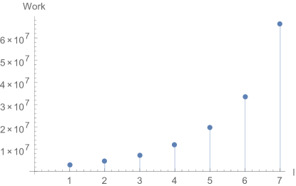
Figure 2. Work distribution among levels. Schematic presentation based on a case of $\beta=0.6$.

4.3. Multilevel Monte Carlo for RDEs

We shall now combine the results of Section 3 and Section 4. For convenience, we recall the regularity assumptions of the convergence analysis (cf. Condition 10): Let $X=(X^{1},\ldots,X^{d})\colon[0,T]\rightarrow\mathbb{R}^{d}$ be a centered, continuous Gaussian process with independent components. Assume that the covariance of every component has finite mixed $(1,\rho)$-variation for some $\rho\in[1,2)$ on $[0,T]^{2}$, that is, for $k=1,\dots,d$,

$$\sup_{\begin{subarray}{c}(t_{i}),(t_{j}^{\prime})\in\mathcal{D}([0,T])\end{subarray}}\left(\sum_{t^{\prime}_{j}}\left(\sum_{t_{i}}\left|E\left[X^{k}_{t_{i},t_{i+1}}X^{k}_{t_{j}^{\prime},t_{j+1}^{\prime}}\right]\right|\right)^{\rho}\right)^{\frac{1}{\rho}}\\ <\infty.$$

Consider the solution $Y\colon[0,T]\to\mathbb{R}^{m}$ of the RDE

$$dY_{t}=V(Y_{t})\,d\mathbf{X}_{t};\quad Y_{0}\in\mathbb{R}^{m}$$

where $V=(V_{1},\ldots,V_{d})$ is a collection of vector fields in $\mathbb{R}^{m}$ with $|V|_{\text{Lip}^{\eta}}<\infty$ for some $\eta\geq\frac{2\rho}{\rho-1}$. Set $S:=Y$ and let $S^{(h_{l})}$ be the simplified step-3 Euler approximation of $Y$ with mesh-size $h_{l}$ (in the case $\rho=1$, it suffices to consider a step-2 approximation). Let $f\colon C([0,T],\mathbb{R}^{m})\to\mathbb{R}^{n}$ be a Lipschitz continuous functional and set $P:=f(S)$, $\widehat{P}_{l}:=f(S^{(h_{l})})$.

Theorem 23.

Consider a functional of an RDE driven by Gaussian signal satisfying the above assumptions, which is evaluated to within a MSE of $\varepsilon^{2}$.
(a) If we assume that the cost of sampling a vector of increments of $X$ of length $N$ is proportional to $N\log(N)$, then an upper bound for the complexity is given by

$$\mathcal{O}\left(\varepsilon^{-\theta}\right),\quad\forall\theta>\frac{2\rho}{2-\rho}.$$

(b) On the other hand, if we assume that the cost of obtaining such a sample is proportional to $N^{2}$, then an upper bound of the total complexity is

$$\mathcal{O}\left(\varepsilon^{-\theta}\right),\quad\forall\theta>\frac{4\rho}{2-\rho}.$$

Proof.

We want to calculate the quantities needed in Theorem 18. As $f$ is assumed to be Lipschitz, the weak rate of convergence is (at least) the strong rate of convergence, i.e., $\alpha=\beta/2$ in the notation of Theorem 18. By Corollary 17, the strong rate is $\beta/2=\frac{2}{\rho}-\frac{1}{2}-\delta$ for any $\delta>0$. Observe that

$$\operatorname{var}\left[\widehat{P}_{l}-P\right]\leq E\left[\left(\widehat{P}_{l}-P\right)^{2}\right]\leq\left|f\right|_{Lip}^{2}E\left[\left|S^{\left(h_{l}\right)}-S\right|^{2}\right]=O\left(h_{l}^{\beta}\right)$$

and

$$\operatorname{var}\left[\widehat{P}_{l}-\widehat{P}_{l-1}\right]\leq\left(\operatorname{var}\left[\widehat{P}_{l}-P\right]^{1/2}+\operatorname{var}\left[\widehat{P}_{l-1}-P\right]^{1/2}\right)^{2}=O\left(h_{l}^{\beta}\right)$$

for all $\beta<\frac{2}{\rho}-1$. Of course the variance of the average of $N_{l}$ IID samples becomes

$$\operatorname{var}\left[\widehat{Y}_{l}\right]=\frac{1}{N_{l}}\operatorname{var}\left[\widehat{P}_{l}-\widehat{P}_{l-1}\right]=O\left(h_{l}^{\beta}/N_{l}\right).$$

This shows condition (iii) in Theorem 18. Trivially, a strong rate is also a weak rate, in the sense that

$$E\left(\widehat{P}_{l}-P\right)\leq E\left[\left(\widehat{P}_{l}-P\right)^{2}\right]^{1/2}=O\left(h_{l}^{\beta/2}\right),$$

which gives condition (i) Condition (ii), “unbiasedness” is obvious for the estimator (14).

In case (a), condition (iv’) of Theorem 20 holds, and the theorem implies that an MSE $\varepsilon^{2}$ can be achieved at cost proportional to

$$\varepsilon^{-\frac{1}{\alpha}}\log(\varepsilon^{-1})=\varepsilon^{-\left(\frac{1}{\frac{1}{\rho}-\frac{1}{2}}+\delta\right)}\log(\varepsilon^{-1})=\varepsilon^{-\left(\frac{2\rho}{2-\rho}+\delta\right)}\log(\varepsilon^{-1})$$

for any $\delta>0$. By choosing $\delta$ slightly larger, we may get rid of the logarithmic term. In the end, we get $\mathcal{O}\left(\varepsilon^{-\theta}\right)$ for any $\theta>\frac{2\rho}{2-\rho}$.

On the other hand, in the general case (b), we rely on Theorem 18 with $\gamma=2$. By similar calculations as above (replacing $1/\alpha$ by $2/\alpha$), we arrive at the result for this case. ∎

Remark 24.

If $X$ is a fractional Brownian motion with Hurst parameter $H>1/4$ (with $\rho=1/(2H)<2$), then we can generate samples of increments at cost proportional to $N\log(N)$ (e.g., by circulant embedding methods, see [Die04]), and we are, hence, in the situation of Theorem 23 (a).

In Table 2 we compare typical asymptotic complexities for RDEs driven by fractional Brownian motion for both the multi-level and the classical Monte Carlo estimators. We distinguish between the “non-regular” regime when $\alpha=\beta/2$ and the more favorable regime when $\alpha=\beta$. Moreover, we have simplified the presentation in Table 2 by neglecting the higher order and logarithmic terms. I.e., any complexity $\varepsilon^{-a}$ in Table 2 should actually be understood as $\varepsilon^{-a-\delta}$ for any $\delta>0$. Thus, when the Hurst parameter is not too small, multi-level can make the difference between a feasible simulation and a quite impossible one. E.g., when $H=2/5$ and the payoff function $f$ is so irregular that the weak rate of convergence is not better than the strong rate of convergence, the complexity for a standard Monte Carlo estimator would be roughly of order $\varepsilon^{-5.33}$, whereas the multi-level version would have complexity roughly of order $\varepsilon^{-3.33}$, which is not much worse than the complexity of a standard Monte Carlo estimator of the usual Brownian motion regime. Admittedly, when $H=1/3$ and one has an irregular payoff, then both standard and multi-level Monte Carlo are very costly computation wise.

	$H=2/5$		$H=1/3$
	MLMC	classical MC	MLMC	classical MC
$\alpha=\beta/2$	$\varepsilon^{-10/3}\approx\varepsilon^{-3.33}$	$\varepsilon^{-16/3}\approx\varepsilon^{-5.33}$	$\varepsilon^{-6}$	$\varepsilon^{-8}$
$\alpha=\beta$	$\varepsilon^{-8/3}\approx\varepsilon^{-2.67}$	$\varepsilon^{-11/3}\approx\varepsilon^{-3.67}$	$\varepsilon^{-4}$	$\varepsilon^{-5}$

Table 2. Comparison of asymptotic complexities for multi-level and classical Monte Carlo for RDEs driven by fractional Brownian motion with Hurst index $H=2/5$ and $H=1/3$. We distinguish between the cases $\alpha=\beta/2$ and $\alpha=\beta$. For this summary, we neglect the “higher order terms”, i.e., we neglect the $\delta$ in $\beta/2=1/\rho-1/2-\delta$. For $H=2/5$, we set $\beta/2=3/10$, and for $H=1/3$ we set $\beta/2=1/6$.

5. Numerical experiments

5.1. A linear, non-smoothing example

Figure 3. Strong and weak error for a fBm with Hurst index $H=0.4$. Dashed line corresponds to the theoretical strong rate of convergence $0.3$, dotted lines show confidence intervals around the error due to the integration error. Weak error corresponds to the functional $f(y):=(|y(1)|-1)^{+}$.

We consider a linear RDE in $\mathbb{R}^{3}$ driven by a two-dimensional fractional Brownian motion with Hurst index $H$. In fact, we consider vector fields $V_{i}(y)=A_{i}y$, $y\in\mathbb{R}^{3}$, $i=1,\,2$, with

$$A_{1}=\begin{pmatrix}0&1&2\\ -1&0&1/2\\ -2&-1/2&0\end{pmatrix},\quad A_{2}=\begin{pmatrix}0&0.7&0.9\\ -0.7&0&1\\ -0.9&-1&0\end{pmatrix}.$$

Note that the matrices $A_{1}$ and $A_{2}$ are anti-symmetric, implying that the sphere $S^{2}$ is invariant under the solution of the SDE. Note that the RDE driven by these vector fields is rather challenging from a numerical point of view, if we try to solve them using general, non-geometric schemes. In particular, in the case $H=1/2$, the equation is non-hypoelliptic and provides a smooth example in which the standard Euler scheme only has weak convergence rate $1/2$. In the case $H\neq 1/2$, we cannot expect any smoothing properties of the solution, either. Formally, further note that the vector fields are unbounded, violating one of our theoretical assumptions.

We implement the simplified Euler scheme (5), where the increments of the fractional Brownian motion were simulated by Hosking’s method, see [Die04]. Hosking’s method is an exact simulation method, i.e., if fed with truly Gaussian random numbers, it will produce samples from the true distribution of increments of the fractional Brownian motion. It is similar to the more obvious simulation method based on the Cholesky factorization of the covariance matrix of the increments, but preferable in terms of memory requirement, especially when grids of sizes of up to $2^{14}=16384$ are considered. As Cholesky’s method, the complexity of simulating the increments of the fractional Brownian motion on a grid with size $M$ is essentially proportional to $M^{2}$, so we are working in the context of Theorem 23 (b).

Starting at $Y_{0}=(1,0,0)$, Figure 3 shows the strong and weak convergence of the scheme for $H=0.4$. More precisely, let $\overline{Y}_{1}^{N}$ denote the result of the scheme based on a uniform grid on $[0,1]$ based on $N$ time-step. Then consider $\overline{Y}_{1}^{2N}$ based on the increments of the same fBm. Then, the lower part of Figure 3 shows the Monte Carlo estimator of $E\left[\left\lvert\overline{Y}^{N}_{1}-\overline{Y}^{2N}_{1}\right\rvert\right]$ plotted against $N$. We, indeed, observe the expected rate of strong convergence, which, due to Theorem 15 is $2H-1/2=0.3$, but only after a prolonged pre-asymptotic phase.

In the upper panel of Figure 3, we plot the weak error for the calculation of $E\left[f\left(Y_{1}\right)\right]$ for the functional

$$f(y):=(|y|-1)^{+}.$$

This implies that $E\left[f\left(Y_{1}\right)\right]=0$, so that we do not need to carry out lengthy calculations in order to find an appropriately accurate reference value. The figure indicates that the rate of the weak error is again equal to the strong rate $0.3$. Note that the same would be true even in the case $H=1/2$, because the Markov semigroup associated to the solution (in the case $H=1/2$) is not smoothing and, in addition, the functional $f$ is non-smooth on $S^{2}$, i.e., with probability $1$. Again, the roughness of the driving signal leads to a remarkably strong pre-asymptotic regime. Indeed, when the grid is too coarse, then the weak approximation error can be huge. Visually, it seems that the asymptotic error analysis accurately describes the true error when the mesh of the grid is at least around $0.02$ for the case $H=0.4$.

Figure 4. Strong and weak error for a fBm with Hurst index $H=0.33$. Dashed line corresponds to the theoretical strong rate of convergence $0.16$, dotted lines show confidence intervals around the error due to the integration error. Weak error corresponds to the functional $f(y):=(|y(1)|-1)^{+}$.

Figure 4 shows strong and weak errors for the same differential equation and the same function $f$, but in the even rougher case $H=0.33$. In this case, the size of the errors for very coarse grids are even larger than for $H=0.4$, and, moreover, the pre-asymptotic phase seems even longer: here the mesh of the grid should probably be at least $0.01$ in order to describe the true computational error by the asymptotic error bounds.

5.2. Multilevel Monte Carlo for the linear example

This long pre-asymptotic phase, in which the computational error is very large, needs to be taken into account when constructing a successful multi-level estimator: indeed, it is advisable to choose the coarsest grid used in the multi-level iteration already within the asymptotic regime. Thus, in the case $H=0.4$, we would recommend to choose $h_{0}\leq 0.02$ for this particular example. This is remarkably different from the standard SDE case, where often $h_{0}$ is chosen to be equal to $T$, i.e., the coarsest grid contains only the start and end points of the interval $[0,T]$. However, when employing this strategy for the fBm example here, the constants in the error bound for the multi-level estimator will completely overshadow the asymptotic convergence rate, to the extent that even for long computation time no “empirical” convergence is exhibited. Indeed, the coarsest levels then combine a large error with an even larger variance, and this combination, while harmless in the asymptotic limit $\varepsilon\to 0$, renders the standard multi-level construction useless.

Fortunately, the picture is completely different when the coarsest grid is chosen to be fine enough, in the current example for $H=0.4$ this means $h_{0}\leq 0.02$. Then the multi-level algorithm requires considerably less computational time for the same MSE tolerance than a classical MC estimator, even for quite moderate levels of the tolerance. For this demonstration, we choose a different function, namely

$$g(y)=|y|\mathbf{1}_{y^{1}>0}.$$

Indeed, the previously used function $f(y)=(|y|-1)^{+}$ has the property that $f(Y_{1})\equiv 0$, so that the variance of $f(\overline{Y}_{1}^{N})$ goes to $0$ when $N\to\infty$. This, however, makes the basic idea of the multi-level approach redundant, as the variance of estimators anyway decrease when the mesh is decreased, even without the telescoping procedure.

A direct comparison of the performance of the classical and the multi-level Monte-Carlo estimator is difficult in our situation, as it is very hard to obtain a reference value, i.e., a “true result”. Moreover, by the same reasoning the coefficients $c_{i}$ in Theorem 18 are very difficult to estimate. Thus, we use the following procedure to test the respective performances:

• Fix $L$, the number of levels in the multi-level procedure, and $h_{0}$, the coarsest grid. Here, we choose $h_{0}=1/64$ and $L=7$. Thus, the finest grid in the multi-level Monte Carlo corresponds to $h_{L}=0.00012=1/8192$. As the fixed $L$ is probably sub-optimal, this choice is disadvantageous to the multi-level algorithm. We also choose the multiplication factor $M=2$ here, and we parametrize the number of paths $N_{l}$ for the level $l$ by the number of paths $N_{0}$ at the coarsest level by some heuristic. In Table 3, we choose $N_{0}=100$. Again, these non-optimal choices favour the classical Monte Carlo estimator.

• Choose the mesh of the classical Monte Carlo estimator to be equal to $h_{L}$, the finest grid in the multi-level hierarchy. This guarantees that both estimators have the same bias – even though we cannot easily estimate this bias due to the absence of a reference value.

• Choose the number of paths in the classical Monte Carlo estimator and the number of paths in the coarsest grid for the multi-level estimator such that the complexity for the classical Monte Carlo estimator is equal to the complexity of the multi-level Monte Carlo estimator. We use an a-priori estimate for the complexity.

  • For the classical Monte Carlo method, the complexity is estimated by the number of trajectories multiplied by the size of the grid.

  • For the multi-level Monte Carlo method, the complexity at a level $l$ is estimated by the product of the size of the finer grid and the number of trajectories for the level. The overall complexity is estimated by the sum of these complexity estimates for the individual levels.

  Note that in practice, this complexity estimate is only given up to a constant of proportionality, which can be checked by comparing run-times on a computer.

• Compute the sample variance for both estimators. If the sample variance for the multi-level Monte Carlo estimator is (significantly) smaller than the sample variance for the classical Monte Carlo estimator, then we, indeed, have demonstrated that the multi-level estimator will have a smaller MSE than the classical Monte Carlo estimator given the same computational budget, i.e., the same complexity.

The nice aspect of this procedure is that it allows a reliable comparison of MSE given a certain complexity, even when the true MSE is not known because of the absence of a reference value. However, we stress again that the multi-level estimator constructed above will certainly not be optimal.In order to take care of the constant in the complexity bound, we also compare the actual run-times as empirical complexity estimates.

	Multilevel	Classical MC
Variance	$1.47\times 10^{-2}$	$1.90\times 10^{-2}$
Time	$0.99$ s	$3.68$ s

Table 3. Variance and run-times for the multi-level and the classical Monte Carlo algorithm for fixed complexity and bias. Calculations are normalized by $N_{0}=100$.

Table 3 finds that for comparable complexity the variance associated to the classical Monte Carlo estimator is considerably lower than the variance of the classical Monte Carlo estimator. It is interesting to note that the classical Monte Carlo estimator takes considerably longer computational time. The reason is that the multi-level algorithm uses the Euler scheme on coarser grids on average than the classical Monte Carlo algorithm. As the complexity for sampling the increments of the fractional Brownian motion increases quadratically in the size of the grid when Hosking’s method is applied, this explains why the computational time is almost four times larger for the classical Monte Carlo method. Note that there are other exact simulation methods with a complexity of order $\mathcal{O}(M\log(M))$ in the grid size $M$, and approximate simulation methods even with order $\mathcal{O}(M)$, see [Die04]. However, at least for the present, linear differential equation, the simulation of the increments of the fBm will always dominate the Euler steps, even when the complexity does only increase linearly. Thus, the conclusions of Table 3 should hold irrespective of the simulation method.

5.3. A fractional Heston model

As a third example, let us consider an application from finance. One of the most popular asset price models is the Heston model, a stochastic volatility model, meaning that the diffusion coefficient of the asset price is itself stochastic. Recently, it has emerged that the stochastic volatility component is rougher than a standard Brownian motion (or a diffusion process) and should be modelled by a fractional Brownian motion or a process driven by a fractional Brownian motion, respectively, see Gatheral, Jaisson and Rosenbaum [GJR14a] and Bayer, Friz and Gatheral [BFG15] and the references therein. Hence, the following fractional Heston model—corresponding to the classical Heston model in Stratonovich formulation for $h=1/2$—, see also Guennoun, Jacquier and Roome [GJR14b], could be considered:

(25a) $$dS_{t} =-\frac{1}{2}\left(v_{t}+\frac{1}{2}\xi\varrho\right)S_{t}dt+\sqrt{v_{t}}S_{t}dW^{1}_{t}$$

(25b) $$dv_{t} =\left(\kappa(\theta-v_{t})-\frac{1}{4}\xi^{2}\right)dt+\xi\sqrt{v_{t}}(\varrho dW^{1}_{t}+\sqrt{1-\varrho^{2}}dW^{2}_{t}),$$

for a standard Brownian motion $W^{1}$ and an independent fractional Brownian motion $W^{2}$ with Hurst index $1/4<H<1/2$. That is, in terms of the RDE (1), we choose the Gaussian process $X_{t}=(W^{1}_{t},W^{2}_{t})$, which satisfies our assumptions with $\rho=1/(2H)$. Note that the driving noise of the price and the variance processes can be correlated using $-1\leq\varrho\leq 1$.

Notice that the fractional Heston model does not satisfy our regularity assumptions in several ways:

• the vector fields are unbounded;

• the vector fields are not differentiable at $v=0$ and not even defined for $v<0$.

Hence, depending on the choice of parameters and initial values $(S_{0},v_{0})$, we may expect the rate to deteriorate. We also need to adjust the scheme in order to preserve positivity of $(S,v)$, in this case by simply taking the positive part after each time step.

On the other hand, one may expect the impact of the Brownian motion $W^{1}$ to be stronger than the impact of the fractional Brownian motion $W^{2}$, especially when considering standard payoff functions depending on the asset price component $S$ only. Thus, the actual error based on a step size $h$ might look like $h^{-1/2}$ and $h^{-1}$ in the strong and weak sense, respectively, when the parameters and initial values are “nice enough” and $h$ is not too small.

Figure 5. Weak and strong error for the fractional Heston model. Solid lines show the empirical errors, dashed lines show regression lines with rates $1.02$ in the weak and $0.42$ in the strong case. Dotted lines show confidence intervals around the solid lines.

We choose model parameters $\kappa=1$, $\theta=0.16$, $\xi=0.2$, $\rho=-0.1$, $H=0.4$. Notice that these parameters easily verify the Feller condition $2\kappa\theta>\xi^{2}$ (which would imply $v_{t}>0$ for $H=1/2$). We further choose $S_{0}=1$, $v_{0}=\theta$ and $r=0$ and consider a European call option with strike price $K=1$.

As expected and shown in Figure 5, we empirically observe first order weak convergence and strong convergence with rate $1/2$—actually, regression gives rates $1.02$ and $0.42$, respectively. This is significantly better than the theoretical (strong) rate $0.3$. We expect the rate to deteriorate eventually, when the number of timesteps is increased even further.

We have also implemented the multilevel Monte Carlo algorithm for the fractional Heston model (using the same parameters as above). We normalize the workload to (roughly) $2\,610\,000$ individual Euler steps—i.e., we set the cost of one Euler step to one. We choose $M_{0}=M=2$ and fix the bias by requiring $h_{L}=\frac{1}{16}.$ Under these normalizations, the single level and multilevel algorithms produce the variances and run times reported in Table 4.

	Multilevel	Classical MC
Variance	$1.9\times 10^{-7}$	$7.4\times 10^{-7}$
Time	$0.88$ s	$0.79$ s

Table 4. Variance and run-times for the multi-level and the classical Monte Carlo algorithm for fixed complexity and bias.

As expected, the multilevel algorithm again clearly outperforms the single level algorithm in producing an estimate with essentially $4$ times smaller variance. We note that the parameters of the multilevel algorithm were based on the observed weak and strong rates of convergence, not the theoretical ones.

Appendix A Elements of rough path theory

We will now very briefly recall the elements of rough paths theory used in this paper. For more details we refer to [FV10b], [LCL07], [LQ02] or [FH14]. Our notation coincides with the one used in [FV10b].

Let $T^{N}(\mathbb{R}^{d})=\mathbb{R}\oplus\mathbb{R}^{d}\oplus(\mathbb{R}^{d}\otimes\mathbb{R}^{d})\oplus\ldots\oplus(\mathbb{R}^{d})^{\otimes N}$ be the truncated step-$N$ tensor algebra. We are concerned with $T^{N}(\mathbb{R}^{d})$-valued paths, as naturally given by iterated integrations of $\mathbb{R}^{d}$-valued smooth paths (“lifted smooth paths”). Such a path $\mathbf{x}$ has natural increments $\mathbf{x}_{s,t}\equiv\mathbf{x}_{s}^{-1}\otimes\mathbf{x}_{t}$. The projection of such a path $\mathbf{x}$ on the first level is an $\mathbb{R}^{d}$-valued path and will be denoted by $\pi_{1}(\mathbf{x})$, the projection to $k$th level is denoted by $\pi_{k}$. Lifted smooth paths actually take values in $G^{N}(\mathbb{R}^{d})\subset T^{N}(\mathbb{R}^{d})$, where $G^{N}(\mathbb{R}^{d})$ denotes the free step-$N$ nilpotent Lie group with $d$ generators. The (left-invariant) Carnot-Caratheodory metric turns $(G^{N}(\mathbb{R}^{d}),d)$ into a metric space.

This already allows (see e.g. [FV10b]) to introduce the most commonly used (homogenous) rough path “norms”

$$\left\|\mathbf{x}\right\|_{p\text{-var;}\left[0,T\right]} = \sup_{\left(t_{i}\right)\subset\left[0,T\right]}\left(\sum_{i}d\left(\mathbf{x}_{t_{i}},\mathbf{x}_{t_{i+1}}\right)^{p}\right)^{1/p},$$

$$\left\|\mathbf{x}\right\|_{1/p\text{-H\"{o}l;}\left[0,T\right]} = \sup_{0\leq s<t\leq T}\frac{d\left(\mathbf{x}_{s},\mathbf{x}_{t}\right)}{\left|t-s\right|^{1/p}},$$

and distances

$$d_{p\text{-var;}\left[0,T\right]}(\mathbf{x},\mathbf{y}) = \left(\sup_{(t_{i})\subset[0,T]}\sum_{i}d\left(\mathbf{x}_{t_{i},t_{i+1}},\mathbf{y}_{t_{i},t_{i+1}}\right)^{p}\right)^{1/p},$$

$$d_{1/p\text{-H\"{o}l;}\left[0,T\right]}(\mathbf{x},\mathbf{y}) = \sup_{0\leq s<t\leq T}\frac{d\left(\mathbf{x}_{s,t},\mathbf{y}_{s,t}\right)}{\left|t-s\right|^{1/p}}$$

where $p\in[1,\infty)$. Define also “inhomogenous” variation and Hölder distances as follows. For $k=$ $1,\ldots,N,$

$$\rho_{p\text{-var;}\left[0,T\right]}^{\left(k\right)}\left(\mathbf{x},\mathbf{y}\right)=\sup_{\left(t_{i}\right)\subset\left[0,T\right]}\left(\sum_{i}\left|\pi_{k}\left(\mathbf{x}_{t_{i},t_{i+1}}-\mathbf{y}_{t_{i},t_{i+1}}\right)\right|^{p/k}\right)^{k/p},$$

and

$$\rho_{p\text{-var;}\left[0,T\right]}\left(\mathbf{x},\mathbf{y}\right)=\max_{k=1,\ldots,N}\rho_{p\text{-var;}\left[0,T\right]}^{\left(k\right)}\left(\mathbf{x},\mathbf{y}\right).$$

Similarly,

$$\rho_{1/p\text{-H\"{o}l;}\left[0,T\right]}^{\left(k\right)}\left(\mathbf{x},\mathbf{y}\right)=\sup_{0\leq s<t\leq T}\frac{\left|\pi_{k}\left(\mathbf{x}_{s,t}-\mathbf{y}_{s,t}\right)\right|}{\left|t-s\right|^{k/p}},$$

and

$$\rho_{1/p\text{-H\"{o}l;}\left[0,T\right]}\left(\mathbf{x},\mathbf{y}\right)=\max_{k=1,\ldots,N}\rho_{1/p\text{-H\"{o}l;}\left[0,T\right]}^{\left(k\right)}\left(\mathbf{x},\mathbf{y}\right).$$

Recall that a control function $\omega$ is a continuous function from $\{\,0\leq s\leq t\leq T\}$ to $[0,\infty)$, for which $\omega(s,t)+\omega(t,u)\leq\omega(s,u)$ holds for every $s\leq t\leq u$. Note that $\omega(s,t)^{1/p}$ is a natural generalization of the quantity $|t-s|^{1/p}$ which appeared in the definition of all “Hölder objects”

$$\left\|\mathbf{x}\right\|_{1/p\text{-H\"{o}l;}\left[0,T\right]},\,\,d_{1/p\text{-H\"{o}l;}\left[0,T\right]}(\mathbf{x},\mathbf{y}),\,\,\rho^{k}_{1/p\text{-H\"{o}l;}\left[0,T\right]}\left(\mathbf{x},\mathbf{y}\right),\,\,\rho_{1/p\text{-H\"{o}l;}\left[0,T\right]}\left(\mathbf{x},\mathbf{y}\right),\,\,$$

defined above. Replacing $|t-s|^{1/p}$ by $\omega(s,t)^{1/p}$ then gives rise to similar norms and distances, denoted by

$$\left\|\mathbf{x}\right\|_{p\text{-}\omega;\left[0,T\right]},\,\,d_{p\text{-}\omega;\left[0,T\right]}(\mathbf{x},\mathbf{y}),\,\,\rho^{k}_{p\text{-}\omega;\left[0,T\right]}\left(\mathbf{x},\mathbf{y}\right),\,\,\rho_{p\text{-}\omega;\left[0,T\right]}\left(\mathbf{x},\mathbf{y}\right).\,\,$$

By definition, a geometric $1/p$-Hölder rough path $\mathbf{x}$ is a path in $T^{\lfloor p\rfloor}(\mathbb{R}^{d})$ which can be approximated by lifts of smooth paths in the $d_{1/p-\text{H\"{o}l}}$ (equivalently: $\rho_{1/p\text{-H\"{o}l}}$) metric; geometric $p$-rough paths are defined similarly (with respect to the variation distance). Necessarily then, any such $\mathbf{x}$ takes values in $G^{\lfloor p\rfloor}(\mathbb{R}^{d})\subset T^{\lfloor p\rfloor}(\mathbb{R}^{d})$. The resulting rough path spaces are know to be Polish and are denoted by

$$C^{0,1/p-\text{H\"{o}l}}_{0}([0,T],G^{\lfloor p\rfloor}(\mathbb{R}^{d}))\quad\text{and}\quad C^{0,p-\text{var}}_{0}([0,T],G^{\lfloor p\rfloor}(\mathbb{R}^{d})).$$

If $V=(V_{i})_{i=1,\ldots,d}$ is a collection of $\operatorname{Lip}^{\gamma}(\mathbb{R}^{e})$ vector fields (in the sense of Stein, cf. [FV10b]) for some $\gamma>p$ and $\mathbf{x}$ is a geometric $p$-rough path, one can make sense of a unique solution $y\colon[0,T]\to\mathbb{R}^{e}$ of the equation

$$dy_{t}=V(y_{t})\,d\mathbf{x}_{t};\quad y_{0}\in\mathbb{R}^{e}$$

and the solution depends (locally Lipschitz) continuously on the driving signal in the inhomogenous rough paths metric.

Acknowledgements

P.F. has received funding from the European Research Council under the European Union’s Seventh Framework Program (FP7/2007-2013) / ERC grant agreement nr. 258237. S.R. was supported by a scholarship from the Berlin Mathematical School (BMS). C. B. and P. F.  acknowledge funding by the DFG grants BA5484/1 and FR2943/2). All authors acknowledge support from the DFG within Research Unit FOR 2402.

This paper contains results of S. Riedel’s Ph.D. dissertation [Rie13, Ch. 6], which was written in collaboration with CB, PKF and JS.

References

- [BFG15] Christian Bayer, Peter Friz, and Jim Gatheral, Pricing under rough volatility, Quantitative Finance (2015), to appear.
- [BSD13] Denis Belomestny, John Schoenmakers, and Fabian Dickmann, Multilevel dual approach for pricing American style derivatives, Finance Stoch. 17 (2013), no. 4, 717–742.
- [CC80] John M. C. Clark and R. J. Cameron, The maximum rate of convergence of discrete approximations for stochastic differential equations, Stochastic differential systems (Proc. IFIP-WG 7/1 Working Conf., Vilnius, 1978), Lecture Notes in Control and Information Sci., vol. 25, Springer, Berlin, 1980, pp. 162–171.
- [CF10] Thomas Cass and Peter K. Friz, Densities for rough differential equations under Hörmander’s condition, Ann. of Math. (2) 171 (2010), no. 3, 2115–2141.
- [CHAN+15] Nathan Collier, Abdul-Lateef Haji-Ali, Fabio Nobile, Erik von Schwerin, and Ra l Tempone, A continuation multilevel monte carlo algorithm, BIT Numerical Mathematics 55 (2015), no. 2, 399–432 (English).
- [CLL13] Thomas Cass, Christian Litterer, and Terry Lyons, Integrability and tail estimates for Gaussian rough differential equations, Ann. Probab. 41 (2013), no. 4, 3026–3050.
- [CQ02] Laure Coutin and Zhongmin Qian, Stochastic analysis, rough path analysis and fractional Brownian motions, Probab. Theory Related Fields 122 (2002), no. 1, 108–140.
- [Dav07] Alexander M. Davie, Differential equations driven by rough paths: an approach via discrete approximation, Appl. Math. Res. Express. AMRX (2007), no. 2, Art. ID abm009, 40.
- [Die04] Ton Dieker, Simulation of fractional Brownian motion, Master’s thesis, University of Twente, 2004.
- [DNT12] Aurélien Deya, Andreas Neuenkirch, and Samy Tindel, A Milstein-type scheme without Lévy area terms for SDEs driven by fractional Brownian motion, Ann. Inst. Henri Poincaré Probab. Stat. 48 (2012), no. 2, 518–550.
- [FGGR16] Peter K. Friz, Benjamin Gess, Archil Gulisashvili, and Sebastian Riedel, The Jain-Monrad criterion for rough paths and applications to random Fourier series and non-Markovian Hörmander theory, Ann. Probab. 44 (2016), no. 1, 684–738.
- [FH14] Peter K. Friz and Martin Hairer, A course on rough paths, Universitext, Springer, Cham, 2014, With an introduction to regularity structures.
- [FR13] Peter K. Friz and Sebastian Riedel, Integrability of (non-)linear rough differential equations and integrals, Stoch. Anal. Appl. 31 (2013), no. 2, 336–358.
- [FR14] Peter Friz and Sebastian Riedel, Convergence rates for the full Gaussian rough paths, Ann. Inst. Henri Poincaré Probab. Stat. 50 (2014), no. 1, 154–194.
- [FV10a] Peter K. Friz and Nicolas B. Victoir, Differential equations driven by Gaussian signals, Ann. Inst. Henri Poincaré Probab. Stat. 46 (2010), no. 2, 369–413.
- [FV10b] by same author, Multidimensional stochastic processes as rough paths, Cambridge Studies in Advanced Mathematics, vol. 120, Cambridge University Press, Cambridge, 2010, Theory and applications.
- [Gil08a] Michael B. Giles, Improved multilevel Monte Carlo convergence using the Milstein scheme, Monte Carlo and quasi-Monte Carlo methods 2006, Springer, Berlin, 2008, pp. 343–358.
- [Gil08b] by same author, Multilevel Monte Carlo path simulation, Oper. Res. 56 (2008), no. 3, 607–617.
- [GJR14a] Jim Gatheral, Thibault Jaisson, and Mathieu Rosenbaum, Volatility is rough, preprint, 2014.
- [GJR14b] Hamza Guennoun, Antoine Jacquier, and Patrick Roome, Asymptotic behaviour of the fractional heston model, preprint, 2014.
- [GS14] Michael B. Giles and Lukasz Szpruch, Antithetic multilevel Monte Carlo estimation for multi-dimensional SDEs without Lévy area simulation, Ann. Appl. Probab. 24 (2014), no. 4, 1585–1620. MR 3211005
- [HP13] Martin Hairer and Natesh S. Pillai, Regularity of laws and ergodicity of hypoelliptic SDEs driven by rough paths, Ann. Probab. 41 (2013), no. 4, 2544–2598.
- [KP92] Peter E. Kloeden and Eckhard Platen, Numerical solution of stochastic differential equations, Applications of Mathematics (New York), vol. 23, Springer-Verlag, Berlin, 1992.
- [LCL07] Terry J. Lyons, Michael Caruana, and Thierry Lévy, Differential equations driven by rough paths, Lecture Notes in Mathematics, vol. 1908, Springer, Berlin, 2007, Lectures from the 34th Summer School on Probability Theory held in Saint-Flour, July 6–24, 2004, With an introduction concerning the Summer School by Jean Picard.
- [LQ02] Terry J. Lyons and Zhongmin Qian, System control and rough paths, Oxford Mathematical Monographs, Oxford University Press, Oxford, 2002, Oxford Science Publications.
- [MGR09] Thomas Müller-Gronbach and Klaus Ritter, Variable subspace sampling and multi-level algorithms, Monte Carlo and quasi-Monte Carlo methods 2008, Springer, Berlin, 2009, pp. 131–156. MR 2743892 (2012e:65012)
- [MN98] M. Matsumoto and T. Nishimura, Mersenne Twister: A 623-dimensionally equidistributed uniform pseudorandom number generator, ACM Trans. on Modeling and Computer Simulation 8 (1998), no. 1, 3–30.
- [Rie13] Sebastian Riedel, Topics in Gaussian rough paths theory, dissertation, Technische Universität Berlin, 2013.
- [SS94] G. Stolovitzky and K. R. Sreenivasan, Kolmogorov’s refined similarity hypotheses for turbulence and general stochastic processes, Rev. Mod. Phys. 66 (1994), no. 1, 229–240.
- [Tal86] Denis Talay, Discrétisation d’une équation différentielle stochastique et calcul approché d’espérances de fonctionnelles de la solution, RAIRO Modél. Math. Anal. Numér. 20 (1986), no. 1, 141–179.