Tree Decomposition based Steiner Tree Computation over Large Graphs

Abstract

In this paper, we present an exact algorithm for the Steiner tree problem. The algorithm is based on certain pre-computed index structures. Our algorithm offers a practical solution for the Steiner tree problems on graphs of large size and bounded number of terminals.

1 Introduction

The Steiner tree problem is a well-studied NP-hard problem, where we have a graph $G=(V,E)$ with costs on the edges given and a set of terminals $S\subseteq V$. The goal is to find a minimum-cost tree in $G$ that connects/contains the terminals. The well-known exact algorithm (parameterized algorithm) is the Dreyfus-Wagner algorithm [4], which follows the dynamic programming paradigm by computing Steiner trees from its minimum subtrees. The exact complexity of the algorithm is $O(|V|\cdot 3^{|S|}+|V|^{2}\cdot 2^{|S|}+|V|^{3})$. Hence if $|S|$ is considered as a constant, the algorithm is tractable.

Recently, new applications over Web information systems such as keyword search and social network analysis emerge and Steiner tree computation is at the core of the algorithms solving these problems [5]. One prominent feature in this scenario is that the graph size is large: the size of social networks or other graph data in the format of XML/RDF can easily reach hundreds of million of vertices. As a consequence, for the Web-scale graph data, the parameter $|V|^{3}$ is dominant and the computation takes prohibitively long time even $|S|$ is considered as a constant. Although efforts have been made, algorithms yielding exact results can only be applied to small size graphs[3].

In this paper, we present an exact algorithm STEIN I by first constructing certain index structures based on the so-called tree decomposition methodology, and then conducting the Steiner tree computation over the index structure. We show that our algorithm achieves the run time of $O(h\cdot(2tw)^{|S|})$ where $tw$ is the treewidth of the graph (see Definition 5), and $h$ is the height of the tree decomposition of $G$ with an upper bound of $|V|$.

Chimani et al. [2] recently proposed an algorithm for Steiner tree computation with the time complexity $O(B_{2tw}^{2}\cdot tw\cdot|V|)$, where $B_{2tw}$ is the Bell number with the upper bound of $(2tw)^{2tw}$. Clearly this algorithm is only applicable to the graphs with bounded treewidth. Notice that finding the optimal treewidth of a graph is an intractable problem [1]. Thus this algorithm has limitations in practice.

2 Preliminaries

An undirected weighted graph is defined as $G=(V,E)$ plus the weight function $w$, where $V$ is the vertex set and $E\subseteq V\times V$ is the edge set. $w:E\rightarrow\mathbb{Q}^{+}$ is the weight function. Let $G=(V,E)$ be a graph. $G_{1}=(V_{1},E_{1})$ and $G_{2}=(V_{2},E_{2})$ be subgraphs of $G$. The union of $G_{1}$ and $G_{2}$, denoted as $G_{1}\cup G_{2}$, is the graph $G^{\prime}=(V^{\prime},E^{\prime})$ where $V^{\prime}=V_{1}\cup V_{2}$ and $E^{\prime}=E_{1}\cup E_{2}$.

Definition 1 (Steiner tree)

Let $G=(V,E)$ be an undirected graph with the weight function $w$. $S\subseteq V$ is a set of terminals. The Steiner tree with respect to $S$, denoted as $ST_{S}$, is a tree spanning the terminals, where $w(ST_{S}):=\sum_{e\in ST_{S}}w(e)$ is minimal.

If the context is clear, we will sometimes use the statement ”$ST_{S}$ has the value of” by meaning that ”the weight of $ST_{S}$ has the value of”. As a running example, consider the graphs illustrated in Figure 1(a), where two graphs are illustrated in the same figure and they distinguish from each other on the weight of the edge $(v_{5},v_{6})$, where graph 1 has the weight 1 and graph 2 has the value 9. Assume $S=\{v_{1},v_{2},v_{3},v_{4}\}$. Steiner tree for Graph 1 has the weight 5 including $(v_{5},v_{6})$ while the Steiner tree for Graph 2 does not include $(v_{5},v_{6})$.

(a) Graph

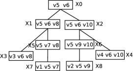
(b) Tree decomposition

Figure 1: Example graphs with $S=\{v_{1},v_{2},v_{3},v_{4}\}$ as terminals and the tree decomposition.

2.1 Algorithm STVS

In this section, we introduce the first Steiner tree algorithm STVS.

Definition 2 (Vertex Separator)

Let $G=(V,E)$ be a graph, $v_{0},v\in V$. $C\subseteq V$ is a $(v_{0},v)$-vertex separator, denoted as $(v_{0},v)$-VS, if for every path $P$ from $v$ to $v_{0}$, there exists a vertex $u$ such that $u\in P$ and $u\in C$.

Theorem 1

Let $G=(V,E)$ be a graph, $v,v_{0}\in V$, $S\subseteq V$ and $S=\{v_{1},\ldots,v_{n}\}$. $C\subseteq V$ is a $(v,v_{0})$-VS. Then

$$ST_{S\cup v_{0}\cup v}={\mbox{min}}~{}~{}~{}ST_{S^{\prime}\cup w\cup v}\cup ST_{S^{\prime\prime}\cup w\cup v_{0}}$$ (1)

where minimum is taken over all $w\in C$ and all bipartitions $S=S^{\prime}\cup S^{\prime\prime}$.

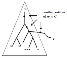
(a) Illustration of Theorem 1

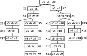
(b) Nice tree decomposition

• Proof. Consider the Steiner tree $ST_{S\cup v_{0}\cup v}$. There must exist a path $P$ from $v$ to $v_{0}$. Given the fact that $C\subseteq V$ is a $(v,v_{0})$-VS, we know that there exists one vertex $w\in C$, such that $w\in P$ as shown in Figure 2(a). No matter where $w$ is located, we can split $ST_{S\cup v_{0}\cup v}$ into two subtrees. One is the subtree rooted at $w$, which contains $v$. The other subtree contains the rest of the terminals in $S$, together with $v_{0}$ and $w$. Each of the subtree is a Steiner tree regarding the terminals. It is trivial to show the minimum of both trees, due to the fact that the entire tree is a Steiner tree.

0:  $G=(V,E)$, $v,v_{0}\in V$, $S=\{v_{1},\ldots,v_{n}\}$, $C\subseteq V$ is a $(v,v_{0})$-VS.

0:  $ST_{S\cup v_{0}\cup v}$ for all vertex $w$ $\in$ $C$   for all $S^{\prime}$, $S^{\prime\prime}$ where $S=S^{\prime}\cup S^{\prime\prime}$        $ST_{S\cup v_{0}\cup v}={\mbox{min}}~{}~{}~{}ST_{S^{\prime}\cup w\cup v}\cup ST_{S^{\prime\prime}\cup w\cup v_{0}}$

  return  $ST_{S\cup v_{0}\cup v}$

Algorithm 1 STVS($v,v_{0},S,C$)

Algorithm 1 shows the pseudo code for computing the Steiner tree according to Theorem 3. The complexity of the algorithm is $|C|\cdot 2^{|S|}$. One important observation about STVS is that the number of terminals of the sub-Steiner trees is not necessarily less than that of the final Steiner tree $ST_{S\cup v_{0}\cup v}$. For instance, take the case of $S^{\prime}=S$ and $S^{\prime\prime}=\emptyset$, the number of terminals of $ST_{S^{\prime}\cup w\cup v}$ is equal to $ST_{S\cup v_{0}\cup v}$ (both are $|S|+2$). Therefore, the dynamic programming paradigm is not applicable in this regard. Moreover, given only the graph, it is unknown how to compute the vertex separator set $C$. If $C$ is not confined in any form (i.e. $C=V$), then STVS becomes an algorithm á la Dreyfus-Wagner. Therefore, in order to make the STVS algorithm useful, it has to be guaranteed that all the sub-Steiner trees be pre-computed, and $C$ be relatively small comparing to $V$. In the following section, we will explain in detail how these conditions are fulfilled with the tree decomposition techniques.

2.2 Tree Decomposition and Treewidth

Definition 3 (Tree Decomposition)

A tree decomposition of a graph $G=(V,E)$, denoted as $T_{G}$, is a pair $(\{X_{i}|i\in I\},T)$, where $I$ is a finite set of integers with the form $\{0,1,\ldots,p\}$ and $\{X_{i}|i\in I\}$ is a collection of subsets of $V$ and $T=(I,F)$ is a tree such that:

1. $\bigcup_{i\in I}X_{i}=V$.

2. for every $(u,v)\in E$, there is $i\in I$, s.t. $u,v\in X_{i}$.

3. for every $v\in V$, the set $\{i|$ v $\in X_{i}\}$ forms a connected subtree of $T$.

A tree decomposition consists of a set of tree nodes, where each node contains a set of vertices in $V$. We call the sets $X_{i}$ bags. It is required that every vertex in $V$ should occur in at least one bag (condition 1), and for every edge in $E$, both vertices of the edge should occur together in at least one bag (condition 2). The third condition is usually referred to as the connectedness condition, which requires that given a vertex $v$ in the graph, all the bags which contain $v$ should be connected.

Note that from now on, the node in the graph $G$ is referred to as vertex, and the node in the tree decomposition is referred to as tree node or simply node. For each tree node $i$, there is a bag $X_{i}$ consisting of vertices. To simplify the representation, we will sometimes use the term node and its corresponding bag interchangeably.

Figure 1(b) illustrates a tree decomposition of the graph from the running example. In most of the tree decomposition related literature, the so-called nice tree decomposition is used. In short, a nice tree decomposition is a tree decomposition, with the following additional conditions: (1) Every internal node $t\in T$ has either 1 or 2 child nodes. (2) If a node $t$ has one child node $t_{0}$, then the bag $X_{t}$ is obtained from $X_{t_{0}}$ either by removing one element or by introducing a new element. (3) If a node $t$ has two child nodes then these child nodes have identical bags as $t$. Given a tree decomposition $T_{G}$, the size of the nice tree decomposition of $T_{G}$ is linear to it. Moreover, the transformation can be done in linear time w.r.t. the size of $T_{G}$. Figure 2(b) shows the nice tree decomposition of the running example graph.

Definition 4 (Induced Subtree)

Let $G=(V,E)$ be a graph and $T_{G}$ its tree decomposition. $v\in V$. The induced subtree of $v$ on $T_{G}$, denoted as $T_{v}$, is a subtree of $T_{G}$ such that for every bag $X\in T_{G}$, $v\in X$ if and only if $X\in T_{v}$.

Intuitively, the induced subtree of a given vertex $v$ consists of precisely those bags that contain $v$. Due to the connectedness condition, $T_{v}$ is a tree. With the definition of induced subtree, any vertex $v$ in the graph $G$ can be uniquely identified with the root of its induced subtree in $T_{G}$. Therefore, from now on we will use the expression of ”the vertex $v$ in $T_{G}$” with the intended meaning that ”the root of the induced subtree of $v$ in $T_{G}$”, if the context is clear.

The following theorem reveals the the relationship between a tree decomposition structure and the vertex separator.

Theorem 2

[6] Let $G=(V,E)$ be a graph and $T_{G}$ its tree decomposition. $u,v\in V$. Every bag $X$ on the path between $u$ and $v$ in $T_{G}$ is a $(u,v)$-vertex separator.

Definition 5 (Width, Treewidth)

Let $G=(V,E)$ be a graph. The width of a tree decomposition $(\{X_{i}|i\in I\},T)$ is defined as $max\{|X_{i}|-1\ |i\in I\}$. The treewidth of $G$ is the minimal width of all tree decompositions of $G$. It is denoted as $tw(G)$ or simply $tw$.

3 STEIN I

Definition 6 (Steiner Tree Set)

Given a set of vertices $S=\{v_{1},\ldots,v_{n}\}$, the Steiner tree Set $\mathcal{ST}_{S}^{m}$ is the set of the Steiner trees of the form $ST_{u_{1},\ldots,u_{k}}$ where $\{u_{1},\ldots,u_{k}\}$ $\subseteq$ $\{v_{1},\ldots,v_{n}\}$ and $2\leq k\leq m$.

Now we are ready to present the algorithm STEIN I, which consists of mainly two parts: (1) Index construction, and (2) Steiner tree query processing. In step (1), we first generate the tree decomposition $T_{G}$ for a given graph $G$. Then for each bag $X$ on $T_{G}$, we compute $\mathcal{ST}_{X}^{l}$, where $l$ is the number of terminals of the Steiner tree computation. In another word, for computing a Steiner tree with $l$ terminals, we need to pre-compute in each bag all the Steiner trees with 2, 3,.$\ldots$, $l$ terminals.

Theorem 3 (STEIN I)

Let $G=(V,E)$ and $T_{G}$ is the tree decomposition of $G$ with treewidth $tw$. $S\subseteq V$ is the terminal set. For every bag $X$ in $T_{G}$, $\mathcal{ST}_{X}^{|S|}$ is pre-computed. Then $ST_{S}$ can be computed in time $O(h\cdot(2tw)^{|S|})$, where $h$ is the height of $T_{G}$.

• Proof. Assume that $T_{G}$ is a nice tree decomposition. First, for each terminal $v_{i}$ we identify the root of the induced subtree $X_{i}$ in $T_{G}$. Then we retrieve the lowest common ancestor (LCA) of all $X_{i}$. We start from the $X_{i}$s, conduct the bottom up traversal from the children nodes to the parent node over $T_{G}$, till LCA is reached.

  Given a bag $X$ in $T_{G}$, we denote all the terminals located in the subtree rooted at $X$ as $S_{X}$. In the following we prove the theorem by induction.

  Claim: Given a bag $X$ in $T_{G}$, if for all its child bags $X_{i}$, $\mathcal{ST}_{X_{i}\cup S_{X_{i}}}^{|S|}$ are computed, then $\mathcal{ST}_{X\cup S_{X}}^{|S|}$ can be computed with the time $O((2tw)^{|S|})$.

  Basis: Bag $X$ is the root of the induced subtree of a terminal $v$, and there is no other terminal below $X$. (That is, $X$ is the one of the bags where we start with.) In this case, $X\cup S_{X}$ = $X$ and $\mathcal{ST}_{X\cup S_{X}}^{|S|}$ = $\mathcal{ST}_{X}^{|S|}$. This is exactly what was pre-computed in bag $X$.

  Induction: In a nice tree decomposition, there are three traversal patterns from the child nodes to the parent node:

  (*) Vertex removal: parent node $X$ has one child node $X_{c}$ where $X_{c}=X\cup v$.

  (*) Vertex insertion: parent node $X$ has one child node $X_{c}$ where $X=X_{c}\cup v$.

(*) Merge: parent node $X$ has two child nodes $X_{c_{1}}$ and $X_{c_{2}}$, where $X$= $X_{c_{1}}$ = $X_{c_{2}}$

Vertex removal. Assume the current parent bag $X$ has the child bag $X_{c}$, such that $X_{c}=X\cup v$ . We observe that $S_{X}$ = $S_{X_{c}}$. That is, the terminal set below $X$ remains the same as with $X_{c}$. This is because from $X_{c}$ to $X$, no new vertex is introduced. There are two cases:

• $v$ is a terminal. Then we need to remember $v$ in $X$. Therefore, we have $\mathcal{ST}_{X\cup S_{X}}^{|S|}$ = $\mathcal{ST}_{X_{c}\setminus v\cup S_{X}\cup v}^{|S|}$ = $\mathcal{ST}_{X_{c}\cup S_{X_{c}}}^{|S|}$. That is, the Steiner tree set in $X$ remains exactly the same as $X_{c}$.

• $v$ is not a terminal. In this case, we remove simply all the Steiner trees from $\mathcal{ST}_{X_{c}\cup S_{X_{c}}}^{|S|}$ where $v$ occurrs as a terminal. This operation costs constant time.

Vertex insertion. Assume the current parent bag $X$ has the child bag $X_{c}$, such that $X=X_{c}\cup v$. First let us consider the inserted vertex $v$ in $X$. Note that $v$ does not occur in $X_{c}$, so according to the connectedness condition, $v$ does not occur in any bag below $X_{c}$. Now consider any terminal $v_{i}$ below $X_{c}$. According to the definition, the root of the induced subtree of $v_{i}$ is also below $X_{c}$. In the following we first prove that $X_{c}$ is a $(v,v_{i})$-vertex separator.

As stated above, $v$ occurs in $X$ and does not occur in $X_{c}$, so we can conclude that the root of the induced subtree of $v$ ($r_{v}$) is an ancestor of $X$. Moreover, we know that the root of the induced subtree of $x_{i}$ ($r_{v_{i}}$) is below $X_{c}$. As a result, $X_{c}$ is in the path between $r_{v}$ and $r_{v_{i}}$. Then according to Theorem 2, $X_{c}$ is a $(v,v_{i})$-vertex separator.

Next we generate all the Steiner trees $ST_{Y\cup v}$, where $Y\subseteq X_{c}\cup S_{X_{c}}$ . We execute the generation of all the Steiner trees in an incremental manner, by inserting the vertices in $X_{c}\cup S_{X_{c}}$ one by one to $v$, starting from the vertices in $X_{c}$, which is then followed by $S_{X_{c}}$. We distinguish the following cases:

• $Y\subseteq X_{c}$. That is, all vertices in $Y$ occurs in $X_{c}$. Obviously $Y\subseteq X$ holds. Then the Steiner tree $ST_{Y\cup v}$ is pre-computed for bag $X$ and we can directly retrieve it.

• $Y\cap S_{X_{c}}\neq\emptyset$. According to the order of the Steiner trees generation above, we assign the newly inserted terminal as $v_{i}$. Let $W=Y\setminus v_{i}$. It is known that $\mathcal{ST}_{W\cup v}^{|S|}$ is already generated. We call the function STVS as follows: STVS$(v_{i},v,W,X_{c})$. Since $X_{c}$ is the $(v_{i},v)$-vertex separator as we shown above, the function will correctly compute the results, as long as all the sub-Steiner trees are available. Let $W=W^{\prime}\cup W^{\prime\prime}$. The first sub-Steiner tree $ST_{W^{\prime}\cup w\cup v_{i}}$ (where $w\in X_{c}$) can be retrieved from the Steiner tree set in $X_{c}$, because there is no $v$ involved. The second sub-Steiner tree has the form $ST_{W^{\prime\prime}\cup w\cup v}$ (where $w\in X_{c}$). It can be retrieved from $\mathcal{ST}_{W\cup v}^{|S|}$, because $W^{\prime\prime}\subseteq W$ and $X_{c}\subseteq W$. The later is true due to the fact that the current step by inserting terminals, all the vertices in $X_{c}$ have already been inserted, according the order of Steiner tree generation we assign. This complete the proof of the correctness.

As far as the complexity is concerned, at each step of vertex insertion, we need to generate $tw^{|S|-1}$ new Steiner trees. Each call of the function of STVS takes time $tw\cdot 2^{|S|}$ in worst case. Thus the total time cost is $tw^{|S|}\cdot 2^{|S|}$ = $(2tw)^{|S|}$.

Merge: Merge operation occurs as bag $X$ has two child nodes $X_{c_{1}}$ and $X_{c_{2}}$, and both children consist of the same set of vertices as $X$. Since each of the child nodes induces a distinct subtree, the terminals below the child nodes are disjunctive.

Basically the step is to merge the Steiner tree sets of both children nodes. Assume the Steiner tree set of both child nodes are $\mathcal{ST}_{X_{c_{1}}\cup S_{X_{c_{1}}}}^{|S|}$ and $\mathcal{ST}_{X_{c_{2}}\cup S_{X_{c_{2}}}}^{|S|}$ respectively, we shall generate the Steiner tree set $\mathcal{ST}_{X\cup S_{X_{c_{1}}}\cup S_{X_{c_{2}}}}^{|S|}$ at the parent node.

The merge operation is analogously to the vertex insertion traversal we introduced above. We start from one child node, say $X_{c_{1}}$. The task is to insert the terminals in $S_{X_{c_{2}}}$ into $\mathcal{ST}_{X_{c_{1}}\cup S_{X_{c_{1}}}}^{|S|}$ one by one. The vertex separator between any terminal in $S_{X_{c_{1}}}$ and $S_{X_{c_{2}}}$ is obviously the bag $X$. The time complexity for the traversal is $(2tw)^{|S|}$ as well.

To conclude, in the bottom up traversal, at each step the Steiner tree set can be computed with the time complexity of $(2tw)^{|S|}$. Since the number of steps is of $O(h\cdot|S|)$, the overall time complexity is $O(h\cdot(2tw)^{|S|})$. This completes the proof.

4 Conclusion

In this paper we presented the algorithm STEIN I, solving the Steiner tree problem over tree decomposed-based index structures. One requirement for the algorithm is that the sub-Steiner trees in the bags have to be pre-computed. However, the computation can be conducted offline. Note that the space for the index storage is $O(tw^{|S|}\cdot|V|)$.

If the number of terminals is considered as a constant, the algorithm is polynomial to the treewidth of the graph $G$, thus the algorithm can also be applied to the graphs whose treewidth is not bounded, but the relationship $tw\ll|V|$ holds. As stated in Introduction, finding $tw$ is an intractable problem. Thus even the treewidth of a graph is bounded, it is unlikely $tw$ can be obtained from a graph of large size. So in practice we can only find certain width $w$, s. t. $w\ll|V|$, which can be achieved for the graphs from Web information systems. There is no obvious correlation between the time complexity and the graph size. In theory, the height of the tree decomposition ($h$) is $\log|V|$ for balanced tree and $|V|$ in worst case. However in practice this value is much smaller than the graph size.

References

- [1] Hans L. Bodlaender. A tourist guide through treewidth. Acta Cybernetica, 11:1–23, 1993.
- [2] Markus Chimani, Petra Mutzel, and Bernd Zey. Improved steiner tree algorithms for bounded treewidth. J. Discrete Algorithms, 16:67–78, 2012.
- [3] Bolin Ding, Jeffrey Xu Yu, Shan Wang, Lu Qin, Xiao Zhang, and Xuemin Lin. Finding top-k min-cost connected trees in databases. In ICDE, 2007.
- [4] S. E. Dreyfus and R. A. Wagner. The Steiner problem in graphs. Networks, 1:195–207, 1972.
- [5] Wen-Syan Li, K. Selçuk Candan, Quoc Vu, and Divyakant Agrawal. Retrieving and organizing web pages by information unit. In Proceedings of the 10th international conference on World Wide Web, 2001.
- [6] Fang Wei. TEDI: efficient shortest path query answering on graphs. In SIGMOD Conference. ACM, 2010.