Convergence to the equilibria for self-stabilizing processes in double-well landscape

Abstract

We investigate the convergence of McKean–Vlasov diffusions in a nonconvex landscape. These processes are linked to nonlinear partial differential equations. According to our previous results, there are at least three stationary measures under simple assumptions. Hence, the convergence problem is not classical like in the convex case. By using the method in Benedetto et al. [J. Statist. Phys. 91 (1998) 1261–1271] about the monotonicity of the free-energy, and combining this with a complete description of the set of the stationary measures, we prove the global convergence of the self-stabilizing processes.

T1Supported by the DFG-funded CRC 701, Spectral Structures and Topological Methods in Mathematics, at the University of Bielefeld.

Introduction

We investigate the weak convergence in long-time of the following so-called self-stabilizing process:

$$\cases{\displaystyle X_{t}=X_{0}+\sqrt{\varepsilon}B_{t}-\int_{0}^{t}V^{\prime}(X_{s})\,ds-\int_{0}^{t}F^{\prime}\ast u_{s}^{\varepsilon}(X_{s})\,ds,\vspace*{2pt}\cr u_{s}^{\varepsilon}=\mathcal{L}(X_{s}).}$$ (I)

Here, $\ast$ denotes the convolution. Since the own law of the process intervenes in the drift, this equation is nonlinear, in the sense of McKean. We note that $X_{t}$ depends on $\varepsilon$. We do not write $\varepsilon$ for simplifying the reading.

The motion of the process is generated by three concurrent forces. The first one is the derivative of a potential $V$—the confining potential. The second influence is a Brownian motion $(B_{t})_{t\in\mathbb{R}_{+}}$. It allows the particle to move upwards the potential $V$. The third term—the so-called self-stabilizing term—represents the attraction between all the others trajectories. Indeed, we remark: $F^{\prime}\ast u_{s}^{\varepsilon}(X_{s}(\omega_{0}))=\int_{\omega\in\Omega}F^{\prime}(X_{s}(\omega_{0})-X_{s}(\omega))\,d\mathbb{P}(\omega)$ where $(\Omega,\mathcal{F},\mathbb{P})$ is the underlying measurable space.

This kind of processes were introduced by McKean, see McKean or McKean1966 . Here, we will make some smoothness assumptions on the interaction potential $F$. Let just note that it is possible to consider nonsmooth $F$. If $F$ is the Heaviside step function and $V:=0$, (I) is the Burgers equation; see SV1979 . If $F:=\delta_{0}$, and without confining potential, it is the Oelschläger equation, studied in Oel1985 .

The particle $X_{t}$ which verifies (I) can be seen as one particle in a continuous mean-field system of an infinite number of particles. The mean-field system that we will consider is a random dynamical system like

$$\cases{\displaystyle dX_{t}^{1}=\sqrt{\varepsilon}\,dB_{t}^{1}-V^{\prime}\bigl{(}X_{t}^{1}\bigr{)}\,dt-\frac{1}{N}\sum_{j=1}^{N}F^{\prime}\bigl{(}X_{t}^{1}-X_{t}^{j}\bigr{)}\,dt,\cr\vdots\cr\displaystyle dX_{t}^{i}=\sqrt{\varepsilon}\,dB_{t}^{i}-V^{\prime}\bigl{(}X_{t}^{i}\bigr{)}\,dt-\frac{1}{N}\sum_{j=1}^{N}F^{\prime}\bigl{(}X_{t}^{i}-X_{t}^{j}\bigr{)}\,dt,\cr\vdots\cr\displaystyle dX_{t}^{N}=\sqrt{\varepsilon}\,dB_{t}^{N}-V^{\prime}\bigl{(}X_{t}^{N}\bigr{)}\,dt-\frac{1}{N}\sum_{j=1}^{N}F^{\prime}\bigl{(}X_{t}^{N}-X_{t}^{j}\bigr{)}\,dt,}$$ (II)

where the $N$ Brownian motions $(B_{t}^{i})_{t\in\mathbb{R}_{+}}$ are independents. Mean-field systems are the subject of a rich literature; see DG1987 for the large deviations for $N\to+\infty$ and M1996 under weak assumptions on $V$ and $F$. For applications, see CDPS2010 for social interactions or CX2010 for the stochastic partial differential equations.

The link between the self-stabilizing process and the mean-field system when $N$ goes to $+\infty$ is called the propagation of chaos; see Sznitman under Lipschitz properties; BRTV if $V$ is a constant; Malrieu2001 or Malrieu2003 when both potentials are convex; BAZ1999 for a more precise result; BGV2007 , DPPH1996 or DG1987 for a sharp estimate; CGM for a uniform result in time in the nonuniformly convex case.

Equation (II) can be rewritten in the following way:

$$d\mathcal{X}_{t}=\sqrt{\varepsilon}\mathcal{B}_{t}-N\nabla\Upsilon^{N}(\mathcal{X}_{t})\,dt,$$ (II)

where the $i$th coordinate of $\mathcal{X}_{t}$ (resp., $\mathcal{B}_{t}$) is $X_{t}^{i}$ (resp., $B_{t}^{i}$) and

$$\Upsilon^{N}(\mathcal{X}):=\frac{1}{N}\sum_{j=1}^{N}V(\mathcal{X}_{j})+\frac{1}{2N^{2}}\sum_{i=1}^{N}\sum_{j=1}^{N}F(\mathcal{X}_{i}-\mathcal{X}_{j})$$

for all $\mathcal{X}\in\mathbb{R}^{N}$. As noted in TT , the potential $\Upsilon^{N}$ converges toward a functional $\Upsilon$ acting on the measures. A perturbation (proportional to $\varepsilon$) of $\Upsilon$ will play the central role in the article.

As observed in DG1987 , the empirical law of the mean-field system can be seen as a perturbation of the law of the diffusion (I). Consequently, the long-time behavior of $\mathcal{L}(X_{t})$ that we study in this paper provides some consequences on the exit time for the particle system (II).

Also, the convergence plays an important role in the exit problem for the self-stabilizing process since the exit time is strongly linked to the drift according to the Kramers law (see DZ or HIP ) which converges toward a homogeneous function if the law of the process converges toward a stationary measure.

Let us recall briefly some of the previous results on diffusions like (I). The existence problem has been investigated by two different methods. The first one consists in the application of a fixed point theorem; see McKean , BRTV , CGM or HIP in the nonconvex case. The other consists of a propagation of chaos; see, for example, M1996 . Moreover, it has been proved in Theorem 2.13 in HIP that there is a unique strong solution.

In McKean , the author proved—by using Weyl’s lemma—that the law of the unique strong solution $du_{t}^{\varepsilon}$ admits a $\mathcal{C}^{\infty}$-continuous density $u_{t}^{\varepsilon}$ with respect to the Lebesgue measure for all $t>0$. Furthermore, this density satisfies a nonlinear partial differential equation of the following type:

$$\frac{\partial}{\partial t}u_{t}^{\varepsilon}(x)=\frac{\partial}{\partial x}\biggl{\{}\frac{\varepsilon}{2}\frac{\partial}{\partial x}u_{t}^{\varepsilon}(x)+u_{t}^{\varepsilon}(x)\bigl{(}V^{\prime}(x)+F^{\prime}\ast u_{t}^{\varepsilon}(x)\bigr{)}\biggr{\}}.$$ (III)

It is then possible to study equations like (III) by probabilistic methods which involve diffusions (I) or (II); see CGM , Funaki1984 , Malrieu2003 . Reciprocally, equation (III) is a useful tool for characterizing the stationary measure(s) and the long-time behavior; see BRTV , BRV , Tamura194 , Tamura1987 , Veret2006 . In HT1 , in the nonconvex case, by using (III), it has been proved that the diffusion (I) admits at least three stationary measures under assumptions easy to verify. One is symmetric, and the two others are not. Moreover, Theorem 3.2 in HT1 states the thirdness of the stationary measures if $V^{\prime\prime}$ is convex and $F^{\prime}$ is linear. This nonuniqueness prevents the long-time behavior from being as intuitive as in the case of unique stationary measure.

The work in HT2 and HT3 provides some estimates of the small-noise asymptotic of these three stationary measures. In particular, the convergence toward Dirac measures and its rate of convergence have been investigated. This will be one of the two main tools for obtaining the convergence.

Convergence for (I) is not a new subject. In BRV , if $V$ is identically equal to $0$, the authors proved the convergence toward the stationary measure by using an ultracontractivity property, a Poincaré inequality and a comparison lemma for stochastic processes. The ultracontractivity property still holds if $V$ is not convex by using the results in KKR . It is possible to conserve the Poincaré inequality by using the theorem of Muckenhoupt (see logsob2000 ) instead of the Bakry–Emery theorem. But, the comparison lemma needs some convexity properties. However, it is possible to apply these results if the initial law is symmetric in the synchronized case ($V^{\prime\prime}(0)+F^{\prime\prime}(0)\geq 0$); see Theorem 7.10 in TT .

Another method consists of using the propagation of chaos in order to derive the convergence of the self-stabilizing process from the one of the mean-field system. However, we shall use it independently of the time and the classical result which is on a finite interval of time is not sufficiently strong. Cattiaux, Guillin and Malrieu proceeded a uniform propagation of chaos in CGM and obtained the convergence in the convex case, including the nonuniformly strictly convex case. See also Malrieu2003 . Nevertheless, according to Proposition 5.17 and Remark 5.18 in TT , it is impossible to find a general result of uniform propagation of chaos. In the synchronized case, if the initial law is symmetric, it is possible to find such a uniform propagation of chaos; see Theorems 7.11 and 7.12 in TT .

The method that we will use in this paper is based on the one of BCCP . See also Malrieu2003 , Tamura194 , Malrieu2001 , HS1987 , AMTU2001 for the convex case. In the nonconvex case, Carrillo, McCann and Villani provide the convergence in CMV2003 under two restrictions: the center of mass is fixed and $V^{\prime\prime}(0)+F^{\prime\prime}(0)>0$ (that means it is the synchronized case).

However, by combining the results in HT1 , HT2 , HT3 with the work of BCCP (and the more rigorous proofs in CMV2003 about the free-energy), we will be able to prove the convergence in a more general setting. The principal tool of the paper is the monotonicity of the free-energy along the trajectories of (III).

First, we introduce the following functional:

$$\Upsilon(u):=\int_{\mathbb{R}}V(x)\,du(x)+\frac{1}{2}\int\!\!\!\int_{\mathbb{R}^{2}}F(x-y)\,du(x)\,du(y).$$ (IV)

This quantity appears intuitively as the limit of the potential in (II) for $N\to+\infty$. We consider now the free-energy of the self-stabilizing process (I),

$$\Upsilon_{\varepsilon}(u):=\frac{\varepsilon}{2}\int_{\mathbb{R}}u(x)\log\bigl{(}u(x)\bigr{)}\,dx+\Upsilon(u)$$

for all measures $du$ which are absolutely continuous with respect to the Lebesgue measure. We can note that $du_{t}^{\varepsilon}$ satisfies this hypothesis for all $t>0$.

The paper is organized as follows. After presenting the assumptions, we will state the first results, in particular, the convergence of a subsequence $(u_{t_{k}}^{\varepsilon})_{k}$. This subconvergence will be used for improving the results about the thirdness of the stationary measures. Then, we will give the main statement which is the convergence toward a stationary measure, briefly discuss the assumptions of the theorem and give the proof. Subsequently, we will study the basins of attraction by two different methods and prove that these basins are not reduced to a single point. Finally, we postpone four results in the annex, including Proposition .2 which extends the classical higher-bound for the moments of the self-stabilizing processes.

Assumptions

We assume the following properties on the confining potential $V$ (see Figure 1): [(V-1)]

$V$ is an even polynomial function with $\deg(V)=:2m\geq 4$.

The equation $V^{\prime}(x)=0$ admits exactly three solutions: $a$, $-a$ and $0$ with $a>0$. Furthermore, $V^{\prime\prime}(a)>0$ and $V^{\prime\prime}(0)<0$. Then, the bottoms of the wells are located in $x=a$ and $x=-a$.

$V(x)\geq C_{4}x^{4}-C_{2}x^{2}$ for all $x\in\mathbb{R}$ with $C_{2},C_{4}>0$.

$\lim_{x\to\pm\infty}V^{\prime\prime}(x)=+\infty$ and $V^{\prime\prime}(x)>0$ for all $x\geq a$.

$V^{\prime\prime}$ is convex.

Initialization: $V(0)=0$.

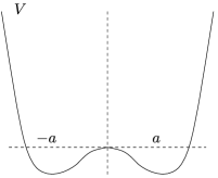
Figure 1: Potential $V$.

Let us remark that the positivity of $V^{\prime\prime}$ on $[-a;a]^{c}$ [in hypothesis (V-4)] is an immediate consequence of (V-1) and (V-5). The simplest and most studied example is $V(x):=\frac{x^{4}}{4}-\frac{x^{2}}{2}$. Also, we would like to stress that weaker assumptions could be considered, but all the mathematical difficulties are present in the polynomial case, and it allows us to avoid some technical and tedious computations. Let us present now the assumptions on the interaction potential $F$: [(F-1)]

$F$ is an even polynomial function with $\deg(F)=:2n\geq 2$.

$F$ and $F^{\prime\prime}$ are convex.

Initialization: $F(0)=0$. Under these assumptions, we know by HT1 that (I) admits at least one symmetric stationary measure. And, if $\sum_{p=0}^{2n-2}\frac{|F^{(p+2)}(a)|}{p!}a^{p}<F^{\prime\prime}(0)+V^{\prime\prime}(a)$, there are at least two asymmetric stationary measures: $u^{\varepsilon}_{+}$ and $u^{\varepsilon}_{-}$. Furthermore, we know by HT2 that there is a unique nonnegative real $x_{0}$ such that $V^{\prime}(x_{0})+\frac{1}{2}F^{\prime}(2x_{0})=0$ and $V^{\prime\prime}(x_{0})+\frac{F^{\prime\prime}(0)+F^{\prime\prime}(2x_{0})}{2}>0$. The same paper provides that $u^{\varepsilon}_{0}$ converges weakly toward $\frac{1}{2}\delta_{x_{0}}+\frac{1}{2}\delta_{-x_{0}}$ and $u^{\varepsilon}_{\pm}$ converges weakly toward $\delta_{\pm a}$ in the small-noise limit.

We present now the assumptions on the initial law $du_{0}$: [(ES)]

The $8q^{2}$th moment of the measure $du_{0}$ is finite with $q:=\max\{m,n\}$.

The probability measure $du_{0}$ admits a $\mathcal{C}^{\infty}$-continuous density $u_{0}$ with respect to the Lebesgue measure. And, the entropy $\int_{\mathbb{R}}u_{0}\log(u_{0})$ is finite. Under (ES), (I) admits a unique strong solution. Indeed, the assumptions of Theorem 2.13 in HIP are satisfied: $V^{\prime}$ and $F^{\prime}$ are locally Lipschitz, $F^{\prime}$ is odd, $F^{\prime}$ grows polynomially, $V^{\prime}$ is continuously differentiable, and there exists a compact $K$ such that $V^{\prime\prime}$ is uniformly negative on $K^{c}$. Moreover, we have the following inequality:

$$\max_{1\leq j\leq 8q^{2}}\sup_{t\in\mathbb{R}_{+}}\mathbb{E}\bigl{[}|X_{t}|^{j}\bigr{]}\leq M_{0}.$$ (V)

We deduce immediately that the family $(u_{t}^{\varepsilon})_{t\in\mathbb{R}_{+}}$ is tight. The assumption (FE) ensures that the initial free-energy is finite. In the following, we shall use occasionally one of the following three additional properties concerning the two potentials $V$ and $F$ and the initial law $du_{0}$: [(SYN)]

$F^{\prime}$ is linear.

$V^{\prime\prime}(0)+F^{\prime\prime}(0)>0$.

For all $N\in\mathbb{N}$, we have $\int_{\mathbb{R}}|x|^{N}\,du_{0}(x)<+\infty$. In the following, three important properties linked to the enumeration of the stationary measures for the self-stabilizing process (I) will be helpful for proving the convergence: [(0M1)]

The process (I) admits exactly three stationary measures. One is symmetric: $u^{\varepsilon}_{0}$ and the other ones are asymmetric: $u^{\varepsilon}_{+}$ and $u^{\varepsilon}_{-}$. Furthermore, $\Upsilon_{\varepsilon}(u^{\varepsilon}_{+})=\Upsilon_{\varepsilon}(u^{\varepsilon}_{-})<\Upsilon_{\varepsilon}(u^{\varepsilon}_{0})$.

There exists $M>0$ such that the diffusion (I) admits exactly three stationary measures with free-energy less than $M$. Furthermore, we have $\Upsilon_{\varepsilon}(u^{\varepsilon}_{+})=\Upsilon_{\varepsilon}(u^{\varepsilon}_{-})<\Upsilon_{\varepsilon}(u^{\varepsilon}_{0})\leq M$ ; $u^{\varepsilon}_{0}$ is symmetric, and $u^{\varepsilon}_{+}$ and $u^{\varepsilon}_{-}$ are asymmetric.

The process (I) admits only one symmetric stationary measure $u^{\varepsilon}_{0}$. In the following, we will give some simple conditions such that (M3), (M3)^′ or (0M1) are true.

Finally, we recall assumption (H) introduced in HT2 :

A family of measures $(v^{\varepsilon})_{\varepsilon}$ verifies assumption (H) if the family of positive reals $(\int_{\mathbb{R}}x^{2n}v^{\varepsilon}(dx))_{\varepsilon>0}$ is bounded. The aim of the weaker assumption (M3)^′ is to obtain the convergence even if there exists a family of stationary measures which does not verify the assumption (H).

For concluding the Introduction, we write the statement of the main theorem:

Let $du_{0}$ be a probability measure which verifies (FE) and (FM). Under (M3), $u_{t}^{\varepsilon}$ converges weakly toward a stationary measure.

1 First results

This section is devoted to present the tools that we will use for proving the main result of the paper. Furthermore, we provide some new results about the thirdness of the stationary measures for the self-stabilizing processes.

We introduce the following functional:

$$\Upsilon_{\varepsilon}^{-}(u):=\frac{\varepsilon}{2}\int_{\mathbb{R}}u(x)\log\bigl{(}u(x)\bigr{)}\mathbh{1}_{\{u(x)<1\}}\,dx+\int_{\mathbb{R}}V(x)u(x)\,dx.$$

This new functional is linked to the free-energy $\Upsilon_{\varepsilon}$. The interaction part and the positive contribution of the entropy term $\int_{\mathbb{R}}u\log(u)$ have been removed. Let us consider a measure $u$ which verifies the previous assumptions. Due to the nonnegativity of the functions $F$ and $x\mapsto\frac{\varepsilon}{2}u(x)\log(u(x))\mathbh{1}_{\{u(x)\geq 1\}}$, we obtain directly the inequality $\Upsilon_{\varepsilon}(u)\geq\Upsilon_{\varepsilon}^{-}(u)$.

In the following, we will need two particular functions [the free-energy of the system and a function $\eta_{t}$ such that $\frac{d}{dt}u_{t}^{\varepsilon}(x)=\frac{d}{dx}\eta_{t}(x)$].

Definition 1.1.

For all $t\in\mathbb{R}_{+}$, we introduce the functions

$$\xi(t):=\Upsilon_{\varepsilon}\bigl{(}u_{t}^{\varepsilon}\bigr{)}\quad\mbox{and}\quad\eta_{t}:=\frac{\varepsilon}{2}\frac{\partial}{\partial x}u_{t}^{\varepsilon}+u_{t}^{\varepsilon}\bigl{(}V^{\prime}+F^{\prime}\ast u_{t}^{\varepsilon}\bigr{)}.\vspace*{-2pt}$$

According to (III), we remark that if $\eta_{t}$ is identically equal to $0$, then $u_{t}^{\varepsilon}$ is a stationary measure for (I).

We recall the following well-known entropy dissipation:

Proposition 1.2

Let $du_{0}$ be a probability measure which verifies (FE) and (ES). Then, for all $t,s\geq 0$, we have

$$\xi(t+s)\leq\xi(t)\leq\xi(0)<+\infty.$$

Furthermore, $\xi$ is derivable, and we have

$$\xi^{\prime}(t)\leq-\int_{\mathbb{R}}\frac{\eta_{t}^{2}}{u_{t}^{\varepsilon}}.\vspace*{-2pt}$$

See CMV2003 for a proof.

1.1 Preliminaries

Let us introduce the functional space

$$\mathcal{M}_{8q^{2}}:=\biggl{\{}f\in\mathcal{C}_{0}^{2}(\mathbb{R},\mathbb{R}_{+})\Big{|}\int_{\mathbb{R}}f(x)\,dx=1\biggr{\}}.$$

We can remark that $u_{t}^{\varepsilon}\in\mathcal{M}_{8q^{2}}$ for all $t>0$; see McKean . The first tool is the Proposition 1.2 [i.e., to say the fact that the free-energy is decreasing along the orbits of (III)]. The second one is its lower-bound.

Lemma 1.3

There exists $\Xi_{v}arepsilon\in\mathbb{R}$ such that $\inf_{u\in\mathcal{M}_{8q^{2}}}\Upsilon_{\varepsilon}(u)\geq\Xi_{\varepsilon}$.

Let us recall $\Upsilon_{\varepsilon}(u)\geq\Upsilon_{\varepsilon}^{-}(u)$. It suffices then to prove the inequality $\inf_{u\in\mathcal{M}_{8q^{2}}}\Upsilon_{\varepsilon}^{-}(u)\geq\Xi_{\varepsilon}$. We proceed as in the first part of the proof of Theorem 2.1 in BCCP . We show that we can minorate the negative part of the entropy by a function of the second moment. Then a growth condition of $V$ will provide the result.

We split the negative part of the entropy into two integrals,

$$-\int_{\mathbb{R}}u(x)\log\bigl{(}u(x)\bigr{)}\mathbh{1}_{\{u(x)<1\}}\,dx=-I_{+}-I_{-}\vspace*{-2pt}$$

with

$$I_{+}:=\int_{\mathbb{R}}u(x)\log\bigl{(}u(x)\bigr{)}\mathbh{1}_{\{e^{-|x|}<u(x)<1\}}\,dx\vspace*{-2pt}$$

and

$$I_{-}:=\int_{\mathbb{R}}u(x)\log\bigl{(}u(x)\bigr{)}\mathbh{1}_{\{u(x)\leq e^{-|x|}\}}\,dx.\vspace*{-2pt}$$

By definition of $I_{+}$, we have the following estimate:

$$I_{+} \geq \int_{\mathbb{R}}u(x)\log\bigl{(}e^{-|x|}\bigr{)}\mathbh{1}_{\{e^{-|x|}<u(x)<1\}}\,dx$$

$$\geq -\int_{\mathbb{R}}|x|u(x)\mathbh{1}_{\{e^{-|x|}<u(x)<1\}}\,dx$$

$$\geq -\int_{\mathbb{R}}|x|u(x)\,dx\geq-\frac{1}{2}-\frac{1}{2}\int_{\mathbb{R}}x^{2}u(x)\,dx.$$

By putting $\gamma(x):=\sqrt{x}\log(x)\mathbh{1}_{\{x<1\}}$, a simple computation provides $\gamma(x)\geq-2e^{-1}$ for all $x<1$. We deduce

$$I_{-}=\int_{\mathbb{R}}\sqrt{u(x)}\gamma\bigl{(}u(x)\bigr{)}\mathbh{1}_{\{u(x)\leq e^{-|x|}\}}\,dx\geq-2e^{-1}\int_{\mathbb{R}}e^{-{|x|}/{2}}\,dx=-8e^{-1}.$$

Consequently, it yields

$$-\int_{\mathbb{R}}u(x)\log\bigl{(}u(x)\bigr{)}\mathbh{1}_{\{u(x)<1\}}\,dx\leq\frac{1}{2}\int_{\mathbb{R}}x^{2}u(x)\,dx+\frac{1}{2}+8e^{-1}.$$

This implies

$$\Upsilon_{\varepsilon}^{-}(u)\geq-\frac{\varepsilon}{4}-4\varepsilon e^{-1}+\int_{\mathbb{R}}\biggl{(}V(x)-\frac{\varepsilon}{4}x^{2}\biggr{)}u(x)\,dx.$$ (1.1)

By hypothesis, there exist $C_{2},C_{4}>0$ such that $V(x)\geq C_{4}x^{4}-C_{2}x^{2}$ so the function $x\mapsto V(x)-\frac{\varepsilon}{4}x^{2}$ is lower-bounded by a negative constant. This achieves the proof. Let us note that the unique assumption we used is $\lim_{x\to\pm\infty}V^{\prime\prime}(x)=+\infty$.

Lemma 1.4

Let $du_{0}$ be a probability measure which satisfies the assumptions (FE) and (ES). Then, there exists $L_{0}\in\mathbb{R}$ such that $\Upsilon_{\varepsilon}(u_{t}^{\varepsilon})$ converges toward $L_{0}$ as time goes to infinity.

The assumption (FE) implies $\xi(0)=\Upsilon_{\varepsilon}(u_{0})<\infty$. As $\xi$ is nonincreasing by Lemma 1.2 and lower-bounded by a constant $\Xi_{\varepsilon}$ according to Lemma 1.3, we deduce that the function $\xi$ converges toward a real $L_{0}$.

Lemma 1.5

If and only if $\xi^{\prime}(t)=0$, the following is true: $u_{t}^{\varepsilon}$ is a stationary measure $u^{\varepsilon}$.

If $u_{t}^{\varepsilon}$ is a stationary measure $u^{\varepsilon}$, then $\xi(t)=\Upsilon_{\varepsilon}(u_{t}^{\varepsilon})=\Upsilon_{\varepsilon}(u^{\varepsilon})$ is a constant. This provides $\xi^{\prime}(t)=0$.

Reciprocally, if $\xi^{\prime}(t)=0$, Proposition 1.2 implies

$$\int_{\mathbb{R}}\frac{\eta_{t}^{2}}{u_{t}^{\varepsilon}}=0.$$

We deduce $\eta_{t}(x)=0$ for all $x\in\mathbb{R}$. This means that $u_{t}^{\varepsilon}$ is a stationary measure.

1.2 Subconvergence

Theorem 1.6

Let $du_{0}$ be a probability measure which satisfies the assumptions (FE) and (ES). Then there exists a stationary measure $u^{\varepsilon}$ and a sequence $(t_{k})_{k}$ which converges toward infinity such that $u_{t_{k}}^{\varepsilon}$ converges weakly toward $u^{\varepsilon}$.

Plan: First, we use the convergence of $\int_{t}^{\infty}\xi^{\prime}(s)\,ds$ toward $0$ when $t$ goes to infinity, and we deduce the existence of a sequence $(t_{k})_{k}$ such that $\xi^{\prime}(t_{k})$ tends toward $0$ when $k$ goes to infinity. Then, we extract a subsequence of $(t_{k})_{k}$ for obtaining an adherence value. By using a test function, we prove that this adherence value is a stationary measure. [Step 1.]

Lemma 1.4 implies that $\int_{t}^{\infty}\xi^{\prime}(s)\,ds$ collapses at infinity. According to Proposition 1.2, the sign of $\xi^{\prime}$ is a constant, so we deduce the existence of an increasing sequence $(t_{k})_{k\in\mathbb{N}}$ which goes to infinity such that $\xi^{\prime}(t_{k})\longrightarrow 0$.

The uniform boundedness of the first $8q^{2}$ moments with respect to the time allows us to use Prohorov’s theorem: we can extract a subsequence [we continue to write it $(t_{k})_{k}$ for simplifying] such that $u_{t_{k}}^{\varepsilon}$ converges weakly toward a probability measure $u^{\varepsilon}$.

We consider now a function $\varphi\in\mathcal{C}^{\infty}(\mathbb{R},\mathbb{R})\cap\mathcal{L}_{2}(u^{\varepsilon})$ with compact support, and we estimate the following quantity:

$$\biggl{|}\int_{\mathbb{R}}\varphi(x)\biggl{\{}\frac{\varepsilon}{2}\frac{\partial}{\partial x}u_{t_{k}}^{\varepsilon}(x)+u_{t_{k}}^{\varepsilon}(x)\bigl{[}V^{\prime}(x)+\bigl{(}F^{\prime}\ast u_{t_{k}}^{\varepsilon}\bigr{)}(x)\bigr{]}\biggr{\}}\,dx\biggr{|}$$

$$\qquad=\biggl{|}\int_{\mathbb{R}}\varphi(x)\eta_{t_{k}}(x)\,dx\biggr{|}=\biggl{|}\int_{\mathbb{R}}\varphi(x)\sqrt{u_{t_{k}}^{\varepsilon}(x)}\frac{|\eta_{t_{k}}(x)|}{\sqrt{u_{t_{k}}^{\varepsilon}(x)}}\,dx\biggr{|}$$

$$\qquad\leq\biggl{(}\int_{\mathbb{R}}\varphi(x)^{2}u_{t_{k}}^{\varepsilon}(x)\,dx\biggr{)}^{{1}/{2}}\times\biggl{(}\int_{\mathbb{R}}\frac{1}{u_{t_{k}}^{\varepsilon}(x)}\bigl{(}\eta_{t_{k}}(x)\bigr{)}^{2}\,dx\biggr{)}^{{1}/{2}}$$

$$\qquad\leq\sqrt{-\xi^{\prime}(t_{k})}\sqrt{\int_{\mathbb{R}}\varphi(x)^{2}u_{t_{k}}^{\varepsilon}(x)}\longrightarrow 0$$

when $k$ goes to infinity; by using the Cauchy–Schwarz inequality, the hypothesis about the sequence $(t_{k})_{k}$, and the weak convergence of $u_{t_{k}}^{\varepsilon}$ toward $u^{\varepsilon}$. The support of $\varphi$ is compact, so we can apply an integration by part to the integral $\int_{\mathbb{R}}\varphi(x)\frac{\partial}{\partial x}u_{t_{k}}^{\varepsilon}(x)\,dx$. Hence, we obtain

$$\int_{\mathbb{R}}\varphi(x)\biggl{\{}\frac{\varepsilon}{2}\frac{\partial}{\partial x}u_{t_{k}}^{\varepsilon}(x)+u_{t_{k}}^{\varepsilon}(x)\bigl{[}V^{\prime}(x)+F^{\prime}\ast u_{t_{k}}^{\varepsilon}(x)\bigr{]}\biggr{\}}\,dx$$

$$\qquad=\int_{\mathbb{R}}\varphi(x)\bigl{[}V^{\prime}(x)+F^{\prime}\ast u_{t_{k}}^{\varepsilon}(x)\bigr{]}u_{t_{k}}^{\varepsilon}(x)\,dx-\int_{\mathbb{R}}\frac{\varepsilon}{2}\varphi^{\prime}(x)u_{t_{k}}^{\varepsilon}(x)\,dx.$$

The weak convergence of $u_{t_{k}}^{\varepsilon}$ to $u^{\varepsilon}$ implies that the previous term tends toward $\int_{\mathbb{R}}\varphi(V^{\prime}+F^{\prime}\ast u^{\varepsilon})u^{\varepsilon}-\int_{\mathbb{R}}\frac{\varepsilon}{2}\varphi^{\prime}u^{\varepsilon}$ when $k$ goes to $\infty$. It has already been proven that $\int_{\mathbb{R}}\varphi\{\frac{\varepsilon}{2}\frac{\partial}{\partial x}u_{t_{k}}^{\varepsilon}+u_{t_{k}}^{\varepsilon}(V^{\prime}+F^{\prime}\ast u_{t_{k}}^{\varepsilon})\}$ is collapsing when $k$ goes to $\infty$. We deduce the following statement:

$$\int_{\mathbb{R}}\varphi\bigl{(}V^{\prime}+F^{\prime}\ast u^{\varepsilon}\bigr{)}u^{\varepsilon}-\int_{\mathbb{R}}\frac{\varepsilon}{2}\varphi^{\prime}u^{\varepsilon}=0.$$ (1.2)

This means that $u^{\varepsilon}$ is a weak solution of the equation

$$\frac{\varepsilon}{2}\frac{\partial}{\partial x}u(x)+\bigl{[}V^{\prime}(x)+F^{\prime}\ast u(x)\bigr{]}u(x)=0.$$

Now, we consider a smooth function $\widetilde{\varphi}$ with compact support $[a,b]$. We put

$$\varphi(x):=\exp\biggl{\{}\frac{2}{\varepsilon}\bigl{[}V(x)+F\ast u^{\varepsilon}(x)\bigr{]}\biggr{\}}\widetilde{\varphi}^{\prime}(x).$$

$\varphi$ is also a smooth function with compact support. Indeed, the application $x\mapsto F\ast u^{\varepsilon}(x)$ is a polynomial function parametrized by the moments of $u^{\varepsilon}$, and these moments are bounded. Equality (1.2) becomes

$$\int_{\mathbb{R}}\widetilde{\varphi}^{\prime\prime}(x)\exp\biggl{\{}\frac{2}{\varepsilon}\bigl{[}V(x)+F\ast u^{\varepsilon}(x)\bigr{]}\biggr{\}}u^{\varepsilon}(x)\,dx=0.$$

By applying Weyl’s lemma, we deduce that $\exp[\frac{2}{\varepsilon}(V+F\ast u^{\varepsilon})]u^{\varepsilon}$ is a smooth function. Moreover, its second derivative is equal to $0$. Then, there exists $A,B\in\mathbb{R}$ such that

$$u^{\varepsilon}(x)=(Ax+B)\exp\biggl{[}-\frac{2}{\varepsilon}\bigl{(}V(x)+F\ast u^{\varepsilon}(x)\bigr{)}\biggr{]}$$

for all $x\in\mathbb{R}$. If $A\neq 0$, it yields $u^{\varepsilon}(-Ax)<0$ for $x$ big enough. This is impossible. Consequently, $u^{\varepsilon}(x)=Z^{-1}\exp[-\frac{2}{\varepsilon}(V(x)+F\ast u^{\varepsilon}(x))]$. This means that $u^{\varepsilon}$ is a stationary measure. ∎

Definition 1.7.

From now on, we call $\mathcal{A}$ the set of the adherence values of the family $(u_{t}^{\varepsilon})_{t\in\mathbb{R}_{+}}$.

Proposition 1.8

With the assumptions and the notation of Theorem 1.6, we have the following limit:

$$L_{0}:=\lim_{t\longrightarrow+\infty}\Upsilon_{\varepsilon}\bigl{(}u_{t}^{\varepsilon}\bigr{)}=\Upsilon_{\varepsilon}\bigl{(}u^{\varepsilon}\bigr{)}.$$

The convergence from the quantity $\int_{\mathbb{R}}Vu_{t_{k}}^{\varepsilon}+\frac{1}{2}\int_{\mathbb{R}}(F\ast u_{t_{k}}^{\varepsilon})u_{t_{k}}^{\varepsilon}$ toward $\int_{\mathbb{R}}Vu^{\varepsilon}+\frac{1}{2}\int_{\mathbb{R}}(F\ast u^{\varepsilon})u^{\varepsilon}$ is a consequence of Theorem 1.6. So we focus on the entropy term.

First of all, we aim to prove that $(u_{t_{k}}^{\varepsilon})_{k}$ is uniformly bounded in the space $W^{1,1}$. For doing this, we will bound the integral on $\mathbb{R}$ of $\frac{\partial}{\partial x}u_{t_{k}}^{\varepsilon}(x)$. The triangular inequality provides

$$\int_{\mathbb{R}}\biggl{|}\frac{\partial}{\partial x}u_{t_{k}}^{\varepsilon}\biggr{|}\leq\frac{2}{\varepsilon}\int_{\mathbb{R}}|\eta_{t_{k}}|+\frac{2}{\varepsilon}\int_{\mathbb{R}}\bigl{|}V^{\prime}+F^{\prime}\ast u_{t_{k}}^{\varepsilon}\bigr{|}u_{t_{k}}^{\varepsilon},$$

where $t\mapsto\eta_{t}$ is defined in Definition 1.1. By using (V) and the growth property of $V^{\prime}$ and $F^{\prime}$, it yields

$$\int_{\mathbb{R}}\bigl{|}V^{\prime}(x)+F^{\prime}\ast u_{t_{k}}^{\varepsilon}(x)\bigr{|}u_{t_{k}}^{\varepsilon}(x)\,dx\leq C_{1}\int_{\mathbb{R}}\bigl{(}1+\bigl{|}x^{2q}\bigr{|}\bigr{)}u_{t_{k}}^{\varepsilon}(x)\,dx\leq C_{2},$$

where $C_{2}$ is a constant. By using the Cauchy–Schwarz inequality, like in the proof of Theorem 1.6, we obtain

$$\int_{\mathbb{R}}\bigl{|}\eta_{t_{k}}(x)\bigr{|}\,dx\leq\sqrt{-\xi^{\prime}(t_{k})}.$$

The quantity $\sqrt{-\xi^{\prime}(t_{k})}$ tends toward $0$, so it is bounded. Finally, it leads to

$$\int_{\mathbb{R}}\biggl{|}\frac{\partial}{\partial x}u_{t_{k}}^{\varepsilon}(x)\biggr{|}\,dx\leq C_{3},$$

where $C_{3}$ is a constant. Consequently, $u_{t_{k}}^{\varepsilon}(x)\leq u_{t_{k}}^{\varepsilon}(0)+C$ for all $x\in\mathbb{R}$. And, since the sequence $(u_{t_{k}}^{\varepsilon}(0))_{k}$ converges, it is bounded, so there exists a constant $C_{4}$ such that $u_{t_{k}}^{\varepsilon}(x)\leq C_{4}$ for all $k\in\mathbb{N}$ and $x\in\mathbb{R}$. It is then easy to prove the convergence of $\int_{\mathbb{R}}u_{t_{k}}^{\varepsilon}(x)\log(u_{t_{k}}^{\varepsilon}(x))\,dx$ toward $\int_{\mathbb{R}}u^{\varepsilon}(x)\log(u^{\varepsilon}(x))\,dx$.

Indeed, the application $x\mapsto u_{t_{k}}^{\varepsilon}(x)\log(u_{t_{k}}^{\varepsilon}(x))$ is lower-bounded, uniformly with respect to $k$. We can then apply the Lebesgue theorem which provides the convergence—when $k$ goes to infinity—of $\int_{\mathbb{R}}u_{t_{k}}^{\varepsilon}(x)\log(u_{t_{k}}^{\varepsilon}(x))\mathbh{1}_{\{|x|\leq R\}}\,dx$ toward $\int_{\mathbb{R}}u^{\varepsilon}(x)\log(u^{\varepsilon}(x))\mathbh{1}_{\{|x|\leq R\}}\,dx$ for all $R\geq 0$. The other integral is split into two terms. The first one is

$$\int_{\mathbb{R}}u_{t_{k}}^{\varepsilon}(x)\log\bigl{(}u_{t_{k}}^{\varepsilon}(x)\bigr{)}\mathbh{1}_{\{|x|>R;u_{t_{k}}^{\varepsilon}(x)\geq 1\}}\,dx \leq \log(C)u_{t_{k}}^{\varepsilon}\bigl{(}[-R;R]^{c}\bigr{)}$$

$$\leq \frac{\log(C)M_{0}}{R^{2}}.$$

The second term is bounded as in the proof of Lemma 1.3:

$$-\int_{\mathbb{R}}u_{t_{k}}^{\varepsilon}(x)\log\bigl{(}u_{t_{k}}^{\varepsilon}(x)\bigr{)}\mathbh{1}_{\{|x|>R;u_{t_{k}}^{\varepsilon}(x)<1\}}\,dx$$

$$\qquad\leq\int_{[-R;R]^{c}}\bigl{\{}|x|u_{t_{k}}^{\varepsilon}(x)-\gamma\bigl{(}u_{t_{k}}^{\varepsilon}(x)\bigr{)}e^{-{|x|}/{2}}\bigr{\}}\,dx\leq\frac{M_{0}}{R}+4e^{-{R}/{2}}.$$

Consequently, $\Upsilon_{\varepsilon}(u_{t_{k}}^{\varepsilon})$ converges toward $\Upsilon_{\varepsilon}(u^{\varepsilon})$, then $\Upsilon_{\varepsilon}(u_{t}^{\varepsilon})$ converges toward $\Upsilon_{\varepsilon}(u^{\varepsilon})$ since the free-energy is monotonous.

By taking $R$ big enough and then $k$ big enough, we can make the following quantity arbitrarily small: $|\int u_{t_{k}}^{\varepsilon}\log(u_{t_{k}}^{\varepsilon})-\int u^{\varepsilon}\log(u^{\varepsilon})|$.

1.3 Consequences

When $V$ is symmetric, Proposition 3.1 (resp., Theorem 4.6) in HT1 states the existence of at least three stationary measures for $\varepsilon$ small enough if $F^{\prime}$ is linear [resp., if $\sum_{p=0}^{\infty}\frac{|F^{(p+2)}(a)|}{p!}a^{p}<F^{\prime\prime}(0)+V^{\prime\prime}(a)$]. Theorem 1.6 permits to extend these results.

Corollary 1.9

For $\varepsilon$ small enough, process (I) admits at least three stationary measures: one is symmetric ($u^{\varepsilon}_{0}$), and two are asymmetric ($u^{\varepsilon}_{+}$ and $u^{\varepsilon}_{-}$). Moreover, for sufficiently small $\varepsilon$, $\Upsilon_{\varepsilon}(u^{\varepsilon}_{+})=\Upsilon_{\varepsilon}(u^{\varepsilon}_{-})<\Upsilon_{\varepsilon}(u^{\varepsilon}_{0})$.

We know by Theorem 4.5 in HT1 that there exists a symmetric stationary measure $u^{\varepsilon}_{0}$. Theorem 5.4 in HT2 implies the weak convergence of $u^{\varepsilon}_{0}$ toward $\frac{1}{2}(\delta_{x_{0}}+\delta_{-x_{0}})$ in the small-noise limit where $x_{0}\in[0;a[$ is the unique solution of

$$\cases{\displaystyle V^{\prime}(x_{0})+\frac{1}{2}F^{\prime}(2x_{0})=0,\vspace*{2pt}\cr\displaystyle V^{\prime\prime}(x_{0})+\frac{F^{\prime\prime}(0)}{2}+\frac{F^{\prime\prime}(2x_{0})}{2}\geq 0.}$$

Lemma .3 provides

$$\lim_{\varepsilon\to 0}\Upsilon_{\varepsilon}\bigl{(}u^{\varepsilon}_{0}\bigr{)}=V(x_{0})+\tfrac{1}{4}F(2x_{0})\quad\mbox{and}\quad\lim_{\varepsilon\to 0}\Upsilon_{\varepsilon}\bigl{(}v^{\varepsilon}_{+}\bigr{)}=V(a)$$

with

$$v^{\varepsilon}_{+}(x):=Z^{-1}\exp\biggl{[}-\frac{2}{\varepsilon}\bigl{(}V(x)+F(x-a)\bigr{)}\biggr{]}.$$

We note that $V(x_{0})+\frac{1}{4}F(2x_{0})>V(a)$. Consequently, for $\varepsilon$ small enough, we have $\Upsilon_{\varepsilon}(v^{\varepsilon}_{+})<\Upsilon_{\varepsilon}(u^{\varepsilon}_{0})$.

We consider now process (I) starting by $u_{0}:=v^{\varepsilon}_{+}$. This is possible because the $8q^{2}$th moment of $v^{\varepsilon}_{+}$ is finite. Theorem 1.6 implies the existence of a sequence $(t_{k})_{k}$ which goes to infinity such that $u_{t_{k}}^{\varepsilon}$ converges weakly toward a stationary measure $u^{\varepsilon}$ satisfying $\Upsilon_{\varepsilon}(u^{\varepsilon})\leq\Upsilon_{\varepsilon}(u_{0})=\Upsilon_{\varepsilon}(v^{\varepsilon}_{+})<\Upsilon_{\varepsilon}(u^{\varepsilon}_{0})$. So $u^{\varepsilon}\neq u^{\varepsilon}_{0}$. We immediately deduce the existence of at least two stationary measures.

If $V^{\prime\prime}(0)+F^{\prime\prime}(0)\neq 0$, we know by Theorem 1.6 in HT3 that there exists a unique symmetric stationary measure for $\varepsilon$ small enough. Hence $u^{\varepsilon}$ is not symmetric.

Let us assume now that $V^{\prime\prime}(0)+F^{\prime\prime}(0)=0$. By (1.1), and by the definition of $\Upsilon_{\varepsilon}^{-}(u)$, we have

$$\Upsilon_{\varepsilon}(u) \geq -\frac{\varepsilon}{4}-4\varepsilon e^{-1}+\int_{\mathbb{R}}\biggl{\{}V(x)-\frac{\varepsilon x^{2}}{4}\biggr{\}}u(x)\,dx$$

$${}+\frac{1}{2}\int\!\!\!\int_{\mathbb{R}^{2}}F(x-y)u(x)u(y)\,dx\,dy$$

for all $u\in\mathcal{M}_{8q^{2}}$. Since $F^{\prime\prime}$ is convex, $x\mapsto F(x)-\frac{F^{\prime\prime}(0)}{2}x^{2}$ is nonnegative. It yields

$$\Upsilon_{\varepsilon}(u) \geq -\frac{\varepsilon}{4}-4\varepsilon e^{-1}+\int_{\mathbb{R}}\biggl{\{}V(x)+\frac{F^{\prime\prime}(0)}{2}x^{2}-\frac{\varepsilon x^{2}}{4}\biggr{\}}u(x)\,dx$$

$${}-\frac{F^{\prime\prime}(0)}{2}\biggl{(}\int_{\mathbb{R}}xu(x)\,dx\biggr{)}^{2}.$$

We deduce the following inequality for all the probability measures satisfying $\int_{\mathbb{R}}xu(x)\,dx=0$:

$$\Upsilon_{\varepsilon}(u)\geq-\frac{\varepsilon}{4}-4\varepsilon e^{-1}+\int_{\mathbb{R}}\biggl{\{}V(x)+\frac{F^{\prime\prime}(0)}{2}x^{2}-\frac{\varepsilon x^{2}}{4}\biggr{\}}u(x)\,dx.$$

In particular, this holds for the symmetric measures. Then, for $\varepsilon$ small enough, $\Upsilon_{\varepsilon}(u)>\frac{V(a)}{2}$ for all the symmetric measures. However, $\Upsilon_{\varepsilon}(v^{\varepsilon}_{+})<\frac{V(a)}{2}$ [then $\Upsilon_{\varepsilon}(u^{\varepsilon})<\frac{V(a)}{2}$] for $\varepsilon$ small enough.

Consequently, the process admits at least one asymmetric stationary measure that we call $u^{\varepsilon}_{+}$. The measure $u^{\varepsilon}_{-}(x):=u^{\varepsilon}_{+}(-x)$ is invariant too. By construction of $u^{\varepsilon}_{+}$ and $u^{\varepsilon}_{-}$, $\Upsilon_{\varepsilon}(u^{\varepsilon}_{+})=\Upsilon_{\varepsilon}^{-}(u^{\varepsilon}_{-})<\Upsilon_{\varepsilon}(u^{\varepsilon}_{0})$.

Remark 1.10.

By a similar method, we could also prove the existence of at least one stationary measure in the asymmetric-landscape case.

We know by Theorem 3.2 in HT1 that if $V^{\prime\prime}$ is convex and if $F^{\prime}$ is linear, there are exactly three stationary measures for $\varepsilon$ small enough. We present a more general setting. In view of the convergence, we will prove that the number of relevant stationary measures is exactly three even if it is a priori possible to imagine the existence of at least four such measures.

Theorem 1.11

We assume $F^{\prime\prime}(0)+V^{\prime\prime}(0)>0$. Then, for all $M>0$, there exists $\varepsilon(M)>0$ such that for all $\varepsilon\leq\varepsilon(M)$, the number of measures $u$ satisfying the two following conditions is exactly three: [(1)]

$u$ is a stationary measure for the diffusion (I).

$\Upsilon_{\varepsilon}(u)\leq M$. Moreover, if $\deg(V)=2m>2n=\deg(F)$, diffusion (I) admits exactly three stationary measures for $\varepsilon$ small enough.

Plan. We will begin to prove the second statement (when $m>n$). For doing this, we will use Corollary 1.9 and the results in HT2 , HT3 . Then, we will prove the first statement by using the second one and a minoration of the free-energy for a sequence of stationary measures which does not verify (H).

[Step 3.2.1.]

Corollary 1.9 implies the existence of $\varepsilon_{0}>0$ such that process (I) admits at least three stationary measures (one is symmetric, and two are asymmetric) if $\varepsilon<\varepsilon_{0}$: $u^{\varepsilon}_{+}$, $u^{\varepsilon}_{-}$ and $u^{\varepsilon}_{0}$.

First, we assume that $\deg(V)>\deg(F)$.

Proposition 3.1 in HT2 implies that each family of stationary measures for the self-stabilizing process (I) verifies condition (H). It has also been shown that under (H), we can extract a subsequence which converges weakly from any family of stationary measures $(u^{\varepsilon})_{\varepsilon>0}$ of the diffusion (I).

Since $F^{\prime\prime}(0)+V^{\prime\prime}(0)>0$, there are three possible limiting values: $\delta_{0}$, $\delta_{a}$ and $\delta_{-a}$ according to Proposition 3.7 and Remark 3.8 in HT2 .

As $F^{\prime\prime}(0)+V^{\prime\prime}(0)>0$ and $V^{\prime\prime}$ and $F^{\prime\prime}$ are convex, there is a unique symmetric stationary measure for $\varepsilon$ small enough by Theorem 1.6 in HT3 . Also, Theorem 1.6 in HT3 implies there are exactly two asymmetric stationary measures for $\varepsilon$ small enough. This achieves the proof of the statement.

Now, we will prove the first statement. First, if $m>n$, by applying the second statement, the result is obvious. We assume now $m\leq n$. Let $M>0$. All the previous results still hold if we restrict the study to the families of stationary measures which verify condition (H). Consequently, it is sufficient to show the following results in order to achieve the proof of the theorem: [(1)]

$\sup\{\Upsilon_{\varepsilon}(u^{\varepsilon}_{0});\Upsilon_{\varepsilon}(u^{\varepsilon}_{+});\Upsilon_{\varepsilon}(u^{\varepsilon}_{-})\}<M$ for $\varepsilon$ small enough.

If $(u^{\varepsilon_{k}})_{k}$ is a sequence of stationary measures, $\int_{\mathbb{R}}x^{2n}u^{\varepsilon_{k}}(x)\,dx\to\infty$ implies $\Upsilon_{\varepsilon_{k}}(u^{\varepsilon_{k}})\to\infty$.

Lemma .3 tells us that $\Upsilon_{\varepsilon}(u^{\varepsilon}_{0})$ [resp., $\Upsilon_{\varepsilon}(u^{\varepsilon}_{+})=\Upsilon_{\varepsilon}(u^{\varepsilon}_{-})$] tends toward $0$ [resp., $V(a)<0$] when $\varepsilon$ goes to $0$. Hence, the first point is obvious.

We will prove the second point. We recall lower-bound (1.1),

$$\Upsilon_{\varepsilon}^{-}(u)\geq-\frac{\varepsilon}{4}-4\varepsilon e^{-1}+\int_{\mathbb{R}}\biggl{(}V(x)-\frac{\varepsilon}{4}x^{2}\biggr{)}u(x)\,dx.$$

As $V(x)\geq C_{4}x^{4}-C_{2}x^{2}$ and $\Upsilon_{\varepsilon}^{-}(u)\leq\Upsilon_{\varepsilon}(u)$ for all smooth $u$, we obtain

$$\Upsilon_{\varepsilon}(u)\geq\int_{\mathbb{R}}x^{2}u(x)\,dx-C,$$

where $C$ is a constant. It is now sufficient to prove that $\int_{\mathbb{R}}x^{2n}u^{\varepsilon_{k}}(x)\,dx\to\infty$ implies $\int_{\mathbb{R}}x^{2}u^{\varepsilon_{k}}(x)\,dx\to\infty$. We will not write the index $k$ for simplifying the reading. We proceed areductio ad absurdum by assuming the existence of a sequence $(u^{\varepsilon})_{\varepsilon}$ which verifies $\int_{\mathbb{R}}x^{2n}u^{\varepsilon}(x)\,dx\to\infty$ and $\int_{\mathbb{R}}x^{2}u^{\varepsilon}(x)\,dx\to C_{+}\in\mathbb{R}_{+}$.

By taking the notation of HT2 , we have the equality $u^{\varepsilon}(x)=Z^{-1}\exp[-\frac{2}{\varepsilon}(W_{\varepsilon}(x))]$ with

$$W_{\varepsilon}(x) := V(x)+F\ast u^{\varepsilon}(x)=\sum_{k=1}^{2n}\omega_{k}(\varepsilon)x^{k}\mbox{,}$$

$$\omega_{k}(\varepsilon) := \frac{1}{k!}\Biggl{\{}V^{(k)}(0)+(-1)^{k}\sum_{j\geq{k}/{2}}^{2n}\frac{F^{(2j)}(0)}{(2j-k)!}m_{2j-k}(\varepsilon)\Biggr{\}}\quad\mbox{and}$$

$$m_{l}(\varepsilon) := \int_{\mathbb{R}}x^{l}u^{\varepsilon}(x)\,dx\qquad\forall l\in\mathbb{N}.$$

We introduce $\omega(\varepsilon):=\sup\{|\omega_{k}(\varepsilon)|^{{1}/{(2n-k)}};1\leq k\leq 2n\}$.

We note that $\omega_{2n}(\varepsilon)=\frac{V^{(2n)}(0)+F^{(2n)}(0)}{(2n)!}>0$. Then, $\omega(\varepsilon)$ is uniformly lower-bounded. Consequently, we can divide by $\omega(\varepsilon)$.

The change of variable $x:=\omega(\varepsilon)y$ provides

$$\frac{m_{2l}(\varepsilon)}{\omega(\varepsilon)^{2l}}=\frac{\int_{\mathbb{R}}y^{2l}\exp[-({2}/{\widehat{\varepsilon}})\widehat{W}^{\varepsilon}(y)]\,dy}{\int_{\mathbb{R}}\exp[-{2}/({\widehat{\varepsilon}})\widehat{W}^{\varepsilon}(y)]\,dy}\qquad\mbox{with }\widehat{W}^{\varepsilon}(x):=\sum_{k=1}^{2n}\frac{\omega_{k}(\varepsilon)}{\omega(\varepsilon)^{2n-k}}x^{k}$$

for all $l\in\mathbb{N}$, with $\widehat{\varepsilon}:=\frac{\varepsilon}{\omega(\varepsilon)^{2n}}$.

The $2n$ sequences $(\frac{\omega_{k}(\varepsilon)}{\omega(\varepsilon)^{2n-k}})_{\varepsilon}$ are bounded so we can extract a subsequence of $\varepsilon$ (we continue to write $\varepsilon$ for simplifying) such that $\frac{\omega_{k}(\varepsilon)}{\omega(\varepsilon)^{2n-k}}$ converges toward $\widehat{\omega}_{k}$ when $\varepsilon\to 0$. We put $\widehat{W}(x):=\sum_{k=1}^{2n}\widehat{\omega}_{k}x^{k}$. We call $A_{1},\ldots,A_{r}$ the $r\geq 1$ location(s) of the global minimum of $\widehat{W}$.

By applying the result of Lemma .4, we can extract a subsequence (and we continue to denote it by $\varepsilon$) such that $\frac{\int_{\mathbb{R}}y^{2l}\exp[-{2}/{\widehat{\varepsilon}}\widehat{W}^{\varepsilon}(y)]\,dy}{\int_{\mathbb{R}}\exp[-{2}/{\widehat{\varepsilon}}\widehat{W}^{\varepsilon}(y)]\,dy}$ converges toward $\sum_{j=1}^{r}p_{j}A_{j}^{2l}$ where $p_{1}+\cdots+p_{r}=1$ and $p_{j}\geq 0$.

If $(\omega(\varepsilon))_{\varepsilon}$ is bounded, since the quantity $\sum_{j=1}^{r}p_{j}A_{j}^{2n}$ is finite, we deduce that $(m_{2n}(\varepsilon))_{\varepsilon}$ is bounded too. Since $m_{2n}(\varepsilon)$ tends toward infinity when $\varepsilon$ goes to $0$, we deduce that $(\omega(\varepsilon))_{\varepsilon}$ converges toward infinity. As $m_{2}(\varepsilon)$ is bounded, the quantity $\frac{m_{2}(\varepsilon)}{\omega(\varepsilon)^{2}}$ vanishes when $\varepsilon$ goes to $0$. This means $\sum_{j=1}^{r}p_{j}A_{j}^{2}=0$ which implies $A_{j}=0$ for all $1\leq j\leq r$. Then $\sum_{j=1}^{r}p_{j}A_{j}^{2n}=0$. Consequently, $m_{2n}(\varepsilon)=o\{\omega(\varepsilon)^{2n}\}$. The Jensen inequality provides $m_{k}(\varepsilon)=o\{\omega(\varepsilon)^{k}\}$.

We recall the definition of $\omega_{k}(\varepsilon)$,

$$\omega_{k}(\varepsilon)=\frac{1}{k!}\Biggl{\{}V^{(k)}(0)+(-1)^{k}\sum_{j\geq{k}/{2}}^{2n}\frac{F^{(2j)}(0)}{(2j-k)!}m_{2j-k}(\varepsilon)\Biggr{\}}.$$

We deduce $\omega_{k}(\varepsilon)=O\{m_{2n-k}(\varepsilon)\}=o\{\omega(\varepsilon)^{2n-k}\}$. So

$$\omega(\varepsilon)=\sup\bigl{\{}\bigl{|}\omega_{k}(\varepsilon)\bigr{|}^{{1}/{(2n-k)}};1\leq k\leq 2n\bigr{\}}=o\bigl{\{}\omega(\varepsilon)\bigr{\}}.$$

This is a contradiction which achieves the proof. ∎ This theorem means that—even if the diffusion (I) admits more than three stationary measures—there are only three stationary measures which play a role in the convergence. Indeed, if we take a measure $u_{0}$ with a finite free-energy, we know that for $\varepsilon$ small enough, there are only three (maybe fewer) stationary measures which can be adherence value of the family $(u_{t}^{\varepsilon})_{t\in\mathbb{R}_{+}}$.

The assumption (LIN) implies (M3) (and (M3)^′ because it is weaker) and (0M1) for $\varepsilon$ small enough. The condition (SYN) implies (M3)^′ and (0M1) for $\varepsilon$ small enough. Furthermore, if $\deg(V)>\deg(F)$, (SYN) implies (M3) when $\varepsilon$ is less than a threshold.

This description of the stationary measures permits us to obtain the principal result, that is to say, the long-time convergence of the process.

2 Global convergence

2.1 Statement of the theorem

We write the main result of the paper:

Theorem 2.1

Let $du_{0}$ be a probability measure which verifies (FE) and (FM). Under (M3), $u_{t}^{\varepsilon}$ converges weakly toward a stationary measure.

The proof is postponed in Section 2.3. First, we will discuss briefly the assumptions.

2.2 Remarks on the assumptions

$du_{0}$ is absolutely continuous with respect to the Lebesgue measure

We shall use Theorem 1.6 and prove that the family $(u_{t}^{\varepsilon})_{t\in\mathbb{R}_{+}}$ admits a unique adherence value. This theorem requires that the initial law is absolutely continuous with respect to the Lebesgue measure. However, it is possible to relax this hypothesis by using the following result (see Lemma 2.1 in HT1 for a proof):

Let $du_{0}$ be a probability measure which verifies $\int_{\mathbb{R}}x^{8q^{2}}\,du_{0}(x)<+\infty$. Then, for all $t>0$, the probability $du_{t}^{\varepsilon}$ is absolutely continuous with respect to the Lebesgue measure.

Consequently, it is sufficient to apply Theorem 2.1 to the probability measure $u_{1}^{\varepsilon}$ since there is a unique solution to the nonlinear equation (I).

The entropy of $du_{0}$ is finite

An essential point of the proof is the convergence of the free-energy. To be sure of this, we assume that it is finite at time $0$. The assumption about the moments implies $\Upsilon_{\varepsilon}(u_{t}^{\varepsilon})<+\infty$ if and only if $\int_{\mathbb{R}}u_{t}^{\varepsilon}\log(u_{t}^{\varepsilon})<+\infty$.

If $V$ was convex, a little adaptation of the theorem in OV2001 (taking into account the fact that the drift is not homogeneous here) would provide the nonoptimal following inequality:

$$\Upsilon_{\varepsilon}\bigl{(}u_{t}^{\varepsilon}\bigr{)}\leq\frac{1}{2t}\inf\bigl{\{}\sqrt{\mathbb{E}|X-Y|^{2}};\mathcal{L}(X)=u_{t}^{\varepsilon};\mathcal{L}(Y)=v_{t}^{\varepsilon}\bigr{\}}$$

with

$$v_{t}^{\varepsilon}(x):=Z^{-1}\exp\biggl{[}-\frac{2}{\varepsilon}\bigl{(}V(x)+F\ast u_{t}^{\varepsilon}(x)\bigr{)}\biggr{]}$$

for all $t>0$. The second moment of $u_{t}^{\varepsilon}$ is upper-bounded uniformly with respect to $t$. By using the convexity of $V$ and $F$, we can prove the same thing for $v_{t}^{\varepsilon}$. Consequently, since $t>0$, the free-energy is finite so the entropy is finite. However, in this paper, we deal with nonconvex landscape, so we will not relax this hypothesis.

All the moments are finite

Theorem 1.6 tells us that we can extract a sequence from the family $(u_{t}^{\varepsilon})_{t\in\mathbb{R}_{+}}$ such that it converges toward a stationary measure. The last step in order to obtain the convergence is the uniqueness of the limiting value. The most difficult part will be to prove this uniqueness when the symmetric stationary measure $u^{\varepsilon}_{0}$ is an adherence value and the only one of these adherence values to be stationary. To do this, we will consider a function like this one:

$$\Phi(u):=\int_{\mathbb{R}}\varphi(x)u(x)\,dx,$$

where $\varphi$ is an odd and smooth function with compact support such that $\varphi(x)=x^{2l+1}$ for all $x$ in a compact subset of $\mathbb{R}$. Then, we will prove—by proceeding a reductio ad absurdum—that there exists an integer $l$ such that $\Phi(u^{\varepsilon}_{0})\neq\Phi(u_{\infty}^{\varepsilon})$, where $u_{\infty}^{\varepsilon}$ would be another limiting value which is a stationary measure. This inequality will allow us to construct a stationary measure $u^{\varepsilon}$ such that $\Phi(u^{\varepsilon})\notin\{\Phi(u^{\varepsilon}_{0});\Phi(u^{\varepsilon}_{+});\Phi(u^{\varepsilon}_{-})\}$. This implies the existence of a stationary measure which does not belong to $\{u^{\varepsilon}_{0};u^{\varepsilon}_{+};u^{\varepsilon}_{-}\}$. Under (M3), it is impossible.

We make the integration with an “almost-polynomial” function because we need the square of the derivative of such function to be uniformly bounded with respect to the time.

However, it is possible to relax the condition (FM). Indeed, according to Proposition .2, if we assume that $\int_{\mathbb{R}}x^{8q^{2}}\,du_{0}(x)<+\infty$ (the condition used for the existence of a strong solution), we have

$$\int_{\mathbb{R}}x^{2l}u_{t}^{\varepsilon}(x)\,dx<+\infty\qquad\forall t>0,l\in\mathbb{N}.$$

Hypothesis (M3)

As written before, the key for proving the uniqueness of the adherence value is to proceed a reductio ad absurdum and then to construct a stationary measure $u^{\varepsilon}$ such that $\Phi(u^{\varepsilon})$ takes a forbidden value [a value different from $\Phi(u^{\varepsilon}_{0})$, $\Phi(u^{\varepsilon}_{+})$ and $\Phi(u^{\varepsilon}_{-})$].

But, it is possible to deal with a weaker hypothesis. Indeed, by considering an initial law with finite free-energy and since the free-energy is decreasing, it is impossible for $u_{t}^{\varepsilon}$ to converge toward a stationary measure with a higher energy. Consequently, we can consider (M3)^′ instead of (M3).

All of these remarks allow us to obtain the following result:

Theorem 2.2

Let $du_{0}$ be a probability measure with finite entropy. If $V$ and $F$ are polynomial functions such that $F^{\prime\prime}(0)+V^{\prime\prime}(0)>0$, $u_{t}^{\varepsilon}$ converges weakly toward a stationary measure for $\varepsilon$ small enough.

2.3 Proof of the theorem

In order to obtain the statement of Theorem 2.1, we will provide two lemmas and one proposition about the free-energy. The lemmas state that a probability measure which verifies simple properties and with a level of energy is necessary a stationary measure for the self-stabilizing process (I). The third one allows us to confine all the adherence values under a level of energy.

Lemma 2.3

Under (M3), if $u$ is a probability measure which satisfies (FE) and (ES), the inequality $\Upsilon_{\varepsilon}(u)\leq\Upsilon_{\varepsilon}(u^{\varepsilon}_{\pm})$ implies $u\in\{u^{\varepsilon}_{+};u^{\varepsilon}_{-}\}$.

Let $u$ be such a measure. We consider the process (I) starting by the initial law $u_{0}:=u$. Theorem 1.6 implies that there exists a stationary measure $u^{\varepsilon}$ such that $\Upsilon_{\varepsilon}(u_{t}^{\varepsilon})$ converges toward $\Upsilon_{\varepsilon}(u^{\varepsilon})$.

However, according to Propositions 1.2 and 1.8,

$$\Upsilon_{\varepsilon}\bigl{(}u^{\varepsilon}\bigr{)}=\lim_{t\to+\infty}\Upsilon_{\varepsilon}\bigl{(}u_{t}^{\varepsilon}\bigr{)}\leq\Upsilon_{\varepsilon}\bigl{(}u_{t}^{\varepsilon}\bigr{)}\leq\Upsilon_{\varepsilon}(u)\leq\Upsilon_{\varepsilon}\bigl{(}u^{\varepsilon}_{\pm}\bigr{)}.$$

Condition (M3) provides $u^{\varepsilon}\in\{u^{\varepsilon}_{+};u^{\varepsilon}_{-};u^{\varepsilon}_{0}\}$. But, $\Upsilon_{\varepsilon}(u^{\varepsilon})\leq\Upsilon_{\varepsilon}(u^{\varepsilon}_{\pm})<\Upsilon_{\varepsilon}(u^{\varepsilon}_{0})$ so $u^{\varepsilon}\in\{u^{\varepsilon}_{+};u^{\varepsilon}_{-}\}$. Without loss of generality, we will assume $u^{\varepsilon}=u^{\varepsilon}_{+}$.

Consequently, the function $\xi$ (see Definition 1.1) is constant. We deduce that $\xi^{\prime}(t)=0$ for all $t\geq 0$. Lemma 1.5 implies that $u_{t}^{\varepsilon}$ is a stationary measure. This means that $u=u_{0}=u^{\varepsilon}=u^{\varepsilon}_{+}$. We have a similar result with the symmetric measures:

Lemma 2.4

Under (0M1), if $u$ is a symmetric probability measure satisfying (FE) and (ES), $\Upsilon_{\varepsilon}(u)\leq\Upsilon_{\varepsilon}(u^{\varepsilon}_{0})$ implies $u=u^{\varepsilon}_{0}$.

The key-argument is the following: if the initial law is symmetric, then the law at time $t$ is still symmetric. The proof is similar to the previous one, so it is left to the reader’s attention.

Before making the convergence, we need a last result on the adherence values: the free-energy of a limiting value is less than the limit value of the free-energy.

Proposition 2.5

We assume that $u_{\infty}^{\varepsilon}$ is an adherence value of the family $(u_{t}^{\varepsilon})_{t\in\mathbb{R}_{+}}$. We call $L_{0}:=\lim_{t\to+\infty}\Upsilon_{\varepsilon}(u_{t}^{\varepsilon})$. Then $\Upsilon_{\varepsilon}(u_{\infty}^{\varepsilon})\leq L_{0}$.

As $u_{\infty}^{\varepsilon}$ is an adherence value of the family $(u_{t}^{\varepsilon})_{t\in\mathbb{R}_{+}}$, there exists an increasing sequence $(t_{k})_{k}$ which goes to infinity such that $u_{t_{k}}^{\varepsilon}$ converges weakly toward $u_{\infty}^{\varepsilon}$. We remark

$$\Upsilon\bigl{(}u_{t_{k}}^{\varepsilon}\bigr{)} = V(a)+\int_{\mathbb{R}}\bigl{(}V(x)-V(a)\bigr{)}u_{t_{k}}^{\varepsilon}(x)\,dx$$

$${}+\frac{1}{2}\int\!\!\!\int_{\mathbb{R}^{2}}F(x-y)u_{t_{k}}^{\varepsilon}(x)u_{t_{k}}^{\varepsilon}(y)\,dx\,dy,$$

where the functional $\Upsilon$ is defined in (IV). As $V(x)-V(a)\geq 0$ for all $x\in\mathbb{R}$, the Fatou lemma implies $\Upsilon(u_{\infty}^{\varepsilon})\leq\liminf_{k\to\infty}\Upsilon(u_{t_{k}}^{\varepsilon})$. In the same way,

$$\int_{\mathbb{R}}u_{\infty}^{\varepsilon}(x)\log\bigl{(}u_{\infty}^{\varepsilon}(x)\bigr{)}\mathbh{1}_{\{u_{\infty}^{\varepsilon}(x)\geq 1\}}\,dx$$

$$\qquad\leq\liminf_{k\to\infty}\int_{\mathbb{R}}u_{t_{k}}^{\varepsilon}(x)\log\bigl{(}u_{t_{k}}^{\varepsilon}(x)\bigr{)}\mathbh{1}_{\{u_{t_{k}}^{\varepsilon}(x)\geq 1\}}\,dx.$$

Let $R>0$. By putting $\gamma_{k}^{-}(x):=u_{t_{k}}^{\varepsilon}(x)\log(u_{t_{k}}^{\varepsilon}(x))\mathbh{1}_{\{u_{t_{k}}^{\varepsilon}(x)<1\}}\mathbh{1}_{\{|x|\leq R\}}$, we note that $|\gamma_{k}^{-}(x)|\leq e^{-1}\mathbh{1}_{\{|x|\leq R\}}$ for all $x\in\mathbb{R}$ and $k\in\mathbb{N}$. We can apply the Lebesgue theorem,

$$\int_{\mathbb{R}}u_{\infty}^{\varepsilon}(x)\log\bigl{(}u_{\infty}^{\varepsilon}(x)\bigr{)}\mathbh{1}_{\{u_{\infty}^{\varepsilon}(x)\geq 1\}}\mathbh{1}_{\{|x|\leq R\}}=\lim_{k\to\infty}\int_{\mathbb{R}}\gamma_{k}^{-}(x)\,dx.$$

We put $\gamma_{k}^{+}(x):=u_{t_{k}}^{\varepsilon}(x)\log(u_{t_{k}}^{\varepsilon}(x))\mathbh{1}_{\{u_{t_{k}}^{\varepsilon}(x)<1\}}\mathbh{1}_{\{|x|>R\}}$. By proceeding as in the proof of Lemma 1.3, we have

$$-\gamma_{k}^{+}(x) = -u_{t_{k}}^{\varepsilon}(x)\log\bigl{(}u_{t_{k}}^{\varepsilon}(x)\bigr{)}\mathbh{1}_{\{e^{-|x|}\leq u_{t_{k}}^{\varepsilon}(x)<1\}}\mathbh{1}_{\{|x|>R\}}$$

$${}-u_{t_{k}}^{\varepsilon}(x)\log\bigl{(}u_{t_{k}}^{\varepsilon}(x)\bigr{)}\mathbh{1}_{\{u_{t_{k}}^{\varepsilon}(x)<e^{-|x|}\}}\mathbh{1}_{\{|x|>R\}}$$

$$\leq |x|u_{t_{k}}^{\varepsilon}(x)\mathbh{1}_{\{|x|>R\}}+2e^{-1}e^{-{|x|}/{2}}\mathbh{1}_{\{|x|>R\}}.$$

Consequently, it leads to the lower-bound

$$\int_{\mathbb{R}}u_{t_{k}}^{\varepsilon}(x)\log\bigl{(}u_{t_{k}}^{\varepsilon}(x)\bigr{)}\mathbh{1}_{\{u_{t_{k}}^{\varepsilon}(x)<1\}}\mathbh{1}_{\{|x|>R\}}\,dx\geq-\frac{M_{0}}{R}-8e^{-1}e^{-{R}/{2}},$$

where $M_{0}$ is defined in (V).

By introducing $\widehat{\Upsilon}_{\varepsilon}(u):=\Upsilon_{\varepsilon}(u)-\frac{\varepsilon}{2}\int_{\mathbb{R}}u(x)\log(u(x))\mathbh{1}_{\{u(x)<1\}}\mathbh{1}_{\{|x|>R\}}\,dx$, we obtain

$$\Upsilon_{\varepsilon}\bigl{(}u_{\infty}^{\varepsilon}\bigr{)}\leq\widehat{\Upsilon}_{\varepsilon}\bigl{(}u_{\infty}^{\varepsilon}\bigr{)} \leq \liminf_{k\to\infty}\widehat{\Upsilon}_{\varepsilon}\bigl{(}u_{t_{k}}^{\varepsilon}\bigr{)}$$

$$\leq \liminf_{k\to\infty}\Upsilon_{\varepsilon}\bigl{(}u_{t_{k}}^{\varepsilon}\bigr{)}+\frac{M_{0}\varepsilon}{2R}+4e^{-1}\exp\biggl{(}-\frac{R}{2}\biggr{)}\varepsilon$$

$$\leq L_{0}+\frac{M_{0}\varepsilon}{2R}+4e^{-1}\varepsilon\exp\biggl{(}-\frac{R}{2}\biggr{)}$$

for all $R>0$. Consequently, $\Upsilon_{\varepsilon}(u_{\infty}^{\varepsilon})\leq L_{0}$. Proof of the theorem Plan: The first step of the proof consists of the application of the Prohorov theorem since the family of measure is tight. We shall prove the uniqueness of the adherence value. We will proceed a reductio ad absurdum. The previous results provide $\mathcal{A}\cap\{u^{\varepsilon}_{0};u^{\varepsilon}_{+};u^{\varepsilon}_{-}\}\neq\varnothing$ where $\mathcal{A}$ is introduced in Definition 1.7. We will then study all the possible cases, and we will prove that all of these cases imply contradictions. If $\mathcal{A}\cap\{u^{\varepsilon}_{0};u^{\varepsilon}_{+};u^{\varepsilon}_{-}\}=\{u^{\varepsilon}_{+}\}$ and $\mathcal{A}\cap\{u^{\varepsilon}_{0};u^{\varepsilon}_{+};u^{\varepsilon}_{-}\}=\{u^{\varepsilon}_{-}\}$ imply contradiction since $u^{\varepsilon}_{+}$ and $u^{\varepsilon}_{-}$ are the unique minimizers of the free-energy. The cases $u^{\varepsilon}_{0}\in\mathcal{A}$ and $\mathcal{A}\cap\{u^{\varepsilon}_{0};u^{\varepsilon}_{+};u^{\varepsilon}_{-}\}=\{u^{\varepsilon}_{+};u^{\varepsilon}_{-}\}$ contradict (M3). [Step 2.1.1.]

Inequality (V) implies that the family of probability measures $\{u_{t}^{\varepsilon};t\in\mathbb{R}_{+}\}$ is tight. Prohorov’s theorem allows us to conclude that each extracted sequence of this family is relatively compact with respect to the weak convergence. So, in order to prove the statement of the theorem, it is sufficient to prove that this family admits exactly one adherence value. We proceed a reductio ad absurdum. We assume in the following that the family admits at least two adherence values.

As condition (M3) is true, there are exactly three stationary measures: $u^{\varepsilon}_{0}$, $u^{\varepsilon}_{+}$ and $u^{\varepsilon}_{-}$. By Theorem 1.6, we know that $\mathcal{A}\cap\{u^{\varepsilon}_{0};u^{\varepsilon}_{+};u^{\varepsilon}_{-}\}\neq\varnothing$. We split this step into three cases:

• $u^{\varepsilon}_{0}\in\mathcal{A}$.

• $\mathcal{A}\cap\{u^{\varepsilon}_{0};u^{\varepsilon}_{+};u^{\varepsilon}_{-}\}=\{u^{\varepsilon}_{+};u^{\varepsilon}_{-}\}$.

• $\mathcal{A}\cap\{u^{\varepsilon}_{0};u^{\varepsilon}_{+};u^{\varepsilon}_{-}\}=\{u^{\varepsilon}_{+}\}$.

By symmetry, we will not deal with the case $\mathcal{A}\cap\{u^{\varepsilon}_{0};u^{\varepsilon}_{+};u^{\varepsilon}_{-}\}=\{u^{\varepsilon}_{-}\}$.

We will prove that the first case, $u^{\varepsilon}_{0}\in\mathcal{A}$, is impossible. It will be the core of the proof.

Let $u_{\infty}^{\varepsilon}$ be an other adherence value of the family $(u_{t}^{\varepsilon})_{t\in\mathbb{R}_{+}}$. Proposition 2.5 tells us $\Upsilon_{\varepsilon}(u_{\infty}^{\varepsilon})\leq\Upsilon_{\varepsilon}(u^{\varepsilon}_{0})$. Since $u_{\infty}^{\varepsilon}\neq u^{\varepsilon}_{0}$, Lemma 2.4 implies that the law $u_{\infty}^{\varepsilon}$ is not symmetric. We deduce that there exists $l\in\mathbb{N}$ such that $\int_{\mathbb{R}}x^{2l+1}u_{\infty}^{\varepsilon}(x)\,dx\neq 0$. Let $R>0$. We introduce the function

$$\varphi(x) := x^{2l+1}\mathbh{1}_{[-R;R]}(x)$$

$${}+x^{2l+1}\mathbh{1}_{[R;R+1]}(x)Z^{-1}\int_{x}^{R+1}\exp\biggl{[}-\frac{1}{(y-R)^{2}}-\frac{1}{(y-R-1)^{2}}\biggr{]}\,dy$$

$${}+x^{2l+1}\mathbh{1}_{[-R-1;-R]}(x)Z^{-1}\int_{-R-1}^{x}\exp\biggl{[}-\frac{1}{(y+R)^{2}}-\frac{1}{(y+R+1)^{2}}\biggr{]}\,dy$$

with

$$Z:=\int_{0}^{1}\exp\biggl{[}-\frac{1}{z^{2}}-\frac{1}{(z-1)^{2}}\biggr{]}\,dz.$$

By construction, $\varphi$ is an odd function, so $\int_{\mathbb{R}}\varphi(x)u^{\varepsilon}_{0}(x)\,dx=0$. Furthermore, $|\varphi(x)|\leq|x|^{2l+1}$. By using the triangular inequality and (FM), we have

$$\biggl{|}\int_{\mathbb{R}}\varphi(x)u_{\infty}^{\varepsilon}(x)\,dx\biggr{|} \geq \biggl{|}\int_{\mathbb{R}}x^{2l+1}u_{\infty}^{\varepsilon}(x)\,dx\biggr{|}-\int_{[-R;R]^{c}}|x|^{2l+1}u_{\infty}^{\varepsilon}(x)\,dx$$

$$\geq \biggl{|}\int_{\mathbb{R}}x^{2l+1}u_{\infty}^{\varepsilon}(x)\,dx\biggr{|}-\frac{1}{R^{3}}C_{0},$$

where $C_{0}:=\sup_{t\in\mathbb{R}_{+}}\int_{\mathbb{R}}|x|^{2l+4}u_{t}^{\varepsilon}(x)\,dx<+\infty$. Since $\int_{\mathbb{R}}x^{2l+1}u_{\infty}^{\varepsilon}(x)\,dx\neq 0$, we deduce that $\int_{\mathbb{R}}\varphi(x)u_{\infty}^{\varepsilon}(x)\,dx\neq 0$ for $R$ big enough. Consequently, we obtain the existence of a smooth function $\varphi$ with compact support such that

$$0=\int_{\mathbb{R}}\varphi(x)u^{\varepsilon}_{0}(x)\,dx<\int_{\mathbb{R}}\varphi(x)u_{\infty}^{\varepsilon}(x)\,dx.$$

Moreover, we can verify that $\varphi^{\prime}(x)^{2}\leq C(R)x^{4l+2}$ for all $x\in\mathbb{R}$. This implies $\sup_{t\in\mathbb{R}_{+}}\int_{\mathbb{R}}\varphi^{\prime}(x)^{2}u_{t}^{\varepsilon}(x)\,dx<+\infty$.

Let $\kappa>0$ such that $|\int_{\mathbb{R}}\varphi(x)u^{\varepsilon}_{+}(x)\,dx|>3\kappa$. By definition of $\mathcal{A}$, there exist two increasing sequences $(t_{k}^{(1)})_{k}$ [resp., $(t_{k}^{(2)})_{k}$] which go to infinity such that $u_{t_{k}^{(1)}}^{\varepsilon}$ [resp., $u_{t_{k}^{(2)}}^{\varepsilon}$] converges weakly toward $u^{\varepsilon}_{0}$ (resp., $u_{\infty}^{\varepsilon}$). We deduce that there exist two increasing sequences $(r_{k})_{k}$ and $(s_{k})_{k}$ such that $\int_{\mathbb{R}}\varphi(x)u_{r_{k}}^{\varepsilon}(x)\,dx=\kappa$ and $\int_{\mathbb{R}}\varphi(x)u_{s_{k}}^{\varepsilon}(x)\,dx=2\kappa$. Then, for all $k\in\mathbb{N}$, we put $\widehat{r}_{k}:=\sup\{t\in[0;s_{k}]|\int_{\mathbb{R}}\varphi(x)u_{t}^{\varepsilon}(x)\,dx=\kappa\}$, and then we define $\widehat{s}_{k}:=\inf\{s\in[\widehat{r}_{k};s_{k}]|\int_{\mathbb{R}}\varphi(x)u_{s}^{\varepsilon}(x)\,dx=2\kappa\}$. For simplifying, we write $r_{k}$ (resp., $s_{k}$) instead of $\widehat{r}_{k}$ (resp., $\widehat{s}_{k}$). And we have

$$\kappa=\int_{\mathbb{R}}\varphi(x)u_{r_{k}}^{\varepsilon}(x)\,dx\leq\int_{\mathbb{R}}\varphi(x)u_{t}^{\varepsilon}(x)\,dx\leq\int_{\mathbb{R}}\varphi(x)u_{s_{k}}^{\varepsilon}(x)\,dx=2\kappa$$

for all $t\in[r_{k};s_{k}]$.

By applying Proposition .1, we deduce that there exists an increasing sequence $(q_{k})_{k}$ going to $+\infty$ such that $(u_{q_{k}}^{\varepsilon})_{k}$ converges weakly toward a stationary measure $u^{\varepsilon}$ verifying $\int_{\mathbb{R}}\varphi(x)u^{\varepsilon}(x)\,dx\in[\kappa;2\kappa]$. Since we have the inequality $|\int_{\mathbb{R}}\varphi(x)u^{\varepsilon}_{+}(x)\,dx|=|\int_{\mathbb{R}}\varphi(x)u^{\varepsilon}_{-}(x)\,dx|>3\kappa$, we deduce $u^{\varepsilon}=u^{\varepsilon}_{0}$. This is impossible since $\int_{\mathbb{R}}\varphi(x)u^{\varepsilon}_{0}(x)\,dx=0\notin[\kappa;2\kappa]$.

We deal now with the third case, $\mathcal{A}\cap\{u^{\varepsilon}_{0};u^{\varepsilon}_{+};u^{\varepsilon}_{-}\}=\{u^{\varepsilon}_{+};u^{\varepsilon}_{-}\}$.

By definition of $u^{\varepsilon}_{+}$ and $u^{\varepsilon}_{-}$, these measures are not symmetric. Consequently, there exists $l\in\mathbb{N}$ such that $\int_{\mathbb{R}}x^{2l+1}u^{\varepsilon}_{+}(x)\,dx\neq 0$. As $u^{\varepsilon}_{-}(x)=u^{\varepsilon}_{+}(-x)$, by proceeding as in Step 2.1, we deduce that there exists an increasing sequence $(q_{k})_{k\in\mathbb{N}}$ which goes to $\infty$ such that $u_{q_{k}}^{\varepsilon}$ converges weakly toward a stationary measure $u^{\varepsilon}$ which verifies $\int_{\mathbb{R}}\varphi u^{\varepsilon}\in[\kappa;2\kappa]$ where $\varphi$ is a smooth function with compact support such that $\int_{\mathbb{R}}\varphi u^{\varepsilon}_{\pm}\notin[\kappa;2\kappa]$. We deduce that $u^{\varepsilon}=u^{\varepsilon}_{0}$ which contradicts $u^{\varepsilon}_{0}\notin\mathcal{A}$.

We consider now the last case, $\mathcal{A}\cap\{u^{\varepsilon}_{0};u^{\varepsilon}_{+};u^{\varepsilon}_{-}\}=\{u^{\varepsilon}_{+}\}$. Proposition 1.8 implies that $\Upsilon_{\varepsilon}(u_{t}^{\varepsilon})$ converges toward $\Upsilon_{\varepsilon}(u^{\varepsilon}_{+})$. Let $u_{\infty}^{\varepsilon}$ be a limit value of the family $(u_{t}^{\varepsilon})_{t\in\mathbb{R}_{+}}$ which is not $u^{\varepsilon}_{+}$. By Proposition 2.5, we know that $\Upsilon_{\varepsilon}(u_{\infty}^{\varepsilon})\leq\Upsilon_{\varepsilon}(u^{\varepsilon}_{+})=\lim_{t\longrightarrow+\infty}\Upsilon_{\varepsilon}(u_{t}^{\varepsilon})$. Then, Lemma 2.3 implies $u_{\infty}^{\varepsilon}=u^{\varepsilon}_{-}\notin\mathcal{A}$.

The family $(u_{t}^{\varepsilon})_{t\in\mathbb{R}_{+}}$ admits only one adherence value with respect to the weak convergence. So $u_{t}^{\varepsilon}$ converges weakly toward a stationary measure which achieves the proof. ∎

3 Basins of attraction

Now we shall provide some conditions in order to precise the limit.

3.1 Domain of $u^{\varepsilon}_{0}$

Theorem 3.1

Let $du_{0}$ be a symmetric probability measure which verifies (FE) and (ES). We assume that $V^{\prime\prime}(0)+F^{\prime\prime}(0)\neq 0$. Then, for $\varepsilon$ small enough $u_{t}^{\varepsilon}$ converges weakly toward $u^{\varepsilon}_{0}$.

$V^{\prime\prime}(0)+F^{\prime\prime}(0)\neq 0$, and both functions $V^{\prime\prime}$ and $F^{\prime\prime}$ are convex. Theorem 1.6 in HT3 implies the existence and the uniqueness of a symmetric stationary measure $u^{\varepsilon}_{0}$ for $\varepsilon$ small enough.

Theorem 1.6 provides the existence of a stationary measure $u^{\varepsilon}$ and an increasing sequence $(t_{k})_{k}$ which goes to $\infty$ such that $u_{t_{k}}^{\varepsilon}$ converges weakly toward $u^{\varepsilon}$ and $\Upsilon_{\varepsilon}(u_{t}^{\varepsilon})$ converges toward $\Upsilon_{\varepsilon}(u^{\varepsilon})$. As $u_{t}^{\varepsilon}$ is symmetric for all $t\geq 0$, we deduce $u^{\varepsilon}=u^{\varepsilon}_{0}$, the unique symmetric stationary measure.

We proceed a reductio ad absurdum by assuming the existence of another sequence $(s_{k})_{k}$ which goes to $\infty$ such that $u_{s_{k}}^{\varepsilon}$ does not converge toward $u^{\varepsilon}_{0}$. The uniform boundedness of the second moment with respect to the time permits to extract a subsequence [we continue to write $(s_{k})_{k}$ for simplifying] such that $u_{s_{k}}^{\varepsilon}$ converges weakly toward $u_{\infty}^{\varepsilon}\neq u^{\varepsilon}_{0}$. Proposition 2.5 implies $\Upsilon_{\varepsilon}(u_{\infty}^{\varepsilon})\leq\Upsilon_{\varepsilon}(u^{\varepsilon}_{0})$. Lemma 2.4 implies $u_{\infty}^{\varepsilon}=u^{\varepsilon}_{0}$. This is absurd.

Remark 3.2.

We assume $V^{\prime\prime}(0)+F^{\prime\prime}(0)\neq 0$ in order to have a unique symmetric stationary measure for $\varepsilon$ small enough, that is to say (0M1). We can extend to the case $V^{\prime\prime}(0)+F^{\prime\prime}(0)=0$ by using auniform propagation of chaos; see Theorem 6.5 in TT . We can also assume that $n=2$ which means $\deg(F)=4$ by Section 4.2 in HT1 .

Remark 3.3.

In the previous theorem, if we assumed (FM) instead of (ES), we could have directly applied Theorem 2.1.

3.2 Domain of $u^{\varepsilon}_{\pm}$

The principal tool of the previous theorem is the stability of a subset (all the symmetric measures with a finite $8q^{2}$-moment). If we could find an invariant subset which contains $u^{\varepsilon}_{+}$, but neither $u^{\varepsilon}_{0}$ nor $u^{\varepsilon}_{-}$, we could apply the same method than previously.

Instead of this, we will consider an inequality linked to the free-energy and we will exhibit a simple subset included in the domain of attraction of $u^{\varepsilon}_{+}$. Let us first introduce the following hyperplan:

$$\mathcal{H}:=\biggl{\{}u\in\mathcal{C}^{\infty}(\mathbb{R};\mathbb{R}_{+})\Big{|}\int_{\mathbb{R}}x^{8q^{2}}u(x)\,dx<\infty\mbox{ and }\int_{\mathbb{R}}xu(x)\,dx=0\biggr{\}}.$$

Theorem 3.4

Let $du_{0}$ be a probability measure which verifies (FE) and (FM). We assume also

$$\Upsilon_{\varepsilon}(u_{0})<\inf_{u\in\mathcal{H}}\Upsilon_{\varepsilon}(u)\quad\mbox{and}\quad\int_{\mathbb{R}}xu_{0}(x)\,dx>0.$$

Under (M3), $u_{t}^{\varepsilon}$ converges weakly toward $u^{\varepsilon}_{+}$.

We know by Theorem 2.1 that there exists a stationary measure $u^{\varepsilon}$ such that $(u_{t}^{\varepsilon})_{t}$ converges weakly toward $u^{\varepsilon}$. And, by Proposition 1.8, $\Upsilon_{\varepsilon}(u_{t}^{\varepsilon})$ converges toward $\Upsilon_{\varepsilon}(u^{\varepsilon})$. [Step 1.]

As $\int_{\mathbb{R}}xu^{\varepsilon}_{0}(x)\,dx=0$ and $\int_{\mathbb{R}}x^{8q^{2}}u^{\varepsilon}_{0}(x)\,dx<+\infty$, we have

$$\Upsilon_{\varepsilon}\bigl{(}u^{\varepsilon}_{0}\bigr{)}\geq\inf_{u\in\mathcal{H}}\Upsilon_{\varepsilon}(u)>\Upsilon_{\varepsilon}(u_{0}).$$

We deduce $u^{\varepsilon}\neq u^{\varepsilon}_{0}$ since $t\mapsto\xi(t)=\Upsilon_{\varepsilon}(u_{t}^{\varepsilon})$ is nonincreasing.

We proceed now a reductio ad absurdum by assuming $u^{\varepsilon}=u^{\varepsilon}_{-}$. There exists $t_{0}>0$ such that $\int_{\mathbb{R}}xu_{t_{0}}^{\varepsilon}(x)\,dx=0$. Consequently,

$$\Upsilon_{\varepsilon}\bigl{(}u_{t_{0}}^{\varepsilon}\bigr{)}\geq\inf_{u\in\mathcal{H}}\Upsilon_{\varepsilon}(u)>\Upsilon_{\varepsilon}(u_{0}),$$

which contradicts the fact that $\xi$ is nonincreasing.

Assumption (M3) implies the weak convergence toward $u^{\varepsilon}_{+}$. ∎ We use now Theorem 3.4 in some particular cases.

Theorem 3.5

Let $du_{0}$ be a probability measure which verifies (FE) and (FM). We assume also

$$\Upsilon(u_{0})<V(x_{0})+\frac{1}{4}F(2x_{0})\quad\mbox{and}\quad\int_{\mathbb{R}}xu_{0}(x)\,dx>0,$$

where $x_{0}$ is defined in the Introduction. Under either conditions (LIN) or (SYN), $u_{t}^{\varepsilon}$ converges weakly toward $u^{\varepsilon}_{+}$ for $\varepsilon$ small enough.

Step 1. Theorem 3.2 in HT1 and Theorem 1.11 imply condition (M3) under (LIN) or (SYN). [Step 2.]

Lemma .3 provides the limit $\lim_{\varepsilon\longrightarrow 0}\Upsilon_{\varepsilon}(u^{\varepsilon}_{0})=V(x_{0})+\frac{1}{4}F(2x_{0})$. Then, we deduce

$$\lim_{\varepsilon\longrightarrow 0}\inf_{u\in\mathcal{H}}\Upsilon_{\varepsilon}(u)\leq V(x_{0})+\frac{1}{4}F(2x_{0}).$$ (3.1)

We prove now that $V(x_{0})+\frac{1}{4}F(2x_{0})=\lim_{\varepsilon\longrightarrow 0}\inf_{u\in\mathcal{H}}\Upsilon_{\varepsilon}(u)$. Indeed, if $u$ is a probability measure such that $\int_{\mathbb{R}}xu(x)\,dx=0$, it verifies the following inequality:

$$\Upsilon_{\varepsilon}(u) \geq \Upsilon_{\varepsilon}^{-}(u)+\frac{F^{\prime\prime}(0)}{4}\int\!\!\!\int_{\mathbb{R}^{2}}(x-y)^{2}u(x)u(y)\,dx\,dy$$

$$\geq \Upsilon_{\varepsilon}^{-}(u)+\frac{F^{\prime\prime}(0)}{2}\int_{\mathbb{R}}x^{2}u(x)\,dx.$$

By using (1.1), it yields

$$\Upsilon_{\varepsilon}(u)\geq-\frac{\varepsilon}{4}-\frac{4\varepsilon}{\exp(1)}+\int_{\mathbb{R}}\biggl{\{}V(x)+\frac{F^{\prime\prime}(0)}{2}x^{2}-\frac{\varepsilon x^{2}}{4}\biggr{\}}u(x)\,dx.$$ (3.2)

We split now the study depending on whether we use conditions (LIN) or (SYN): [(SYN)]

If $F^{\prime}$ is linear, $\frac{F^{\prime\prime}(0)}{2}x^{2}=\frac{1}{4}F(2x)$. So the minimum of $x\mapsto V(x)+\frac{1}{4}F(2x)$ is $V(x_{0})+\frac{1}{4}F(2x_{0})$. We can easily prove that

$$\min_{x\in\mathbb{R}}\biggl{(}V(x)+\frac{F^{\prime\prime}(0)}{2}x^{2}-\frac{\varepsilon}{4}x^{2}\biggr{)}=V(x_{0})+\frac{1}{4}F(2x_{0})+o(1).$$

Consequently,

$$\Upsilon_{\varepsilon}(u)\geq-\frac{\varepsilon}{4}-\frac{4\varepsilon}{\exp(1)}+V(x_{0})+\frac{1}{4}F(2x_{0})+o(1)$$

for all $u\in\mathcal{H}$. Then, $\lim_{\varepsilon\longrightarrow 0}\min_{u\in\mathcal{H}}\Upsilon_{\varepsilon}(u)\geq V(x_{0})+\frac{1}{4}F(2x_{0})$. Inequality (3.1) provides $\lim_{\varepsilon\longrightarrow 0}\inf_{u\in\mathcal{H}}\Upsilon_{\varepsilon}(u)=V(x_{0})+\frac{1}{4}F(2x_{0})$.

Since $V^{\prime\prime}(0)+F^{\prime\prime}(0)>0$, (3.2) implies $\Upsilon_{\varepsilon}(u)\geq-\frac{\varepsilon}{4}-\frac{4\varepsilon}{\exp(1)}$ for all $u\in\mathcal{H}$ if $\varepsilon$ is less than $2(V^{\prime\prime}(0)+F^{\prime\prime}(0))$. We deduce that$\lim_{\varepsilon\longrightarrow 0}\inf_{u\in\mathcal{H}}\Upsilon_{\varepsilon}(u)\geq 0$. However, as $V^{\prime\prime}(0)+F^{\prime\prime}(0)>0$, Theorem 5.4 in HT2 implies $x_{0}=0$ so $V(x_{0})+\frac{1}{4}F(2x_{0})=0$. Inequality (3.1) provides the following limit: $\lim_{\varepsilon\longrightarrow 0}\inf_{u\in\mathcal{H}}\Upsilon_{\varepsilon}(u)=0=V(x_{0})+\frac{1}{4}F(2x_{0})$.

Consequently, $\Upsilon_{\varepsilon}(u_{0})<\inf_{u\in\mathcal{H}}\Upsilon_{\varepsilon}(u)$ for $\varepsilon$ small enough. Then, we apply Theorem 3.4. ∎

Remark 3.6.

We can replace $\int_{\mathbb{R}}xu_{0}(x)\,dx>0$ by $\int_{\mathbb{R}}xu_{0}(x)\,dx<0$ in Theorems 3.4 and 3.5; then the same results hold with $u^{\varepsilon}_{-}$ instead of $u^{\varepsilon}_{+}$.

Appendix: Useful technical results

In this annex, we present some results used previously in the proofs of the main theorems.

Proposition .1 allows us to ensure that even if the free-energy does not reach its global minimum on the stationary measure $u^{\varepsilon}_{0}$, if the unique symmetric stationary measure is an adherence value, then it is unique.

Proposition .2 is a general result on the self-stabilizing processes. Indeed, it is well known that $du_{t}^{\varepsilon}$ is absolutely continuous with respect to the Lebesgue measure for all $t>0$. Proposition .2 extends this instantaneous regularization to the finiteness of all the moments.

Lemma .3 consists in asymptotic computation of the free-energy in the small-noise limit for some useful measures. Lemma .4 use a Laplace method for making a tedious computation which is necessary for avoiding to assume that each family of stationary measures verify condition (H).

We present now the essential proposition for proving Theorem 2.1.

Proposition .1.

Let $du_{0}$ be a probability measure which verifies (FE) and (FM). We assume the existence of two polynomial functions $\mathcal{P}$ and $\mathcal{Q}$, a smooth function $\varphi$ with compact support such that $|\varphi(x)|\leq\mathcal{P}(x)$ and $|\varphi^{\prime}(x)|^{2}\leq\mathcal{Q}(x)$, $\kappa>0$ and two sequences $(r_{k})_{k}$ and $(s_{k})_{k}$ which go to $\infty$ such that for all $r_{k}\leq t\leq s_{k}<r_{k+1}$,

$$\kappa=\int_{\mathbb{R}}\varphi(x)u_{r_{k}}^{\varepsilon}(x)\,dx\leq\int_{\mathbb{R}}\varphi(x)u_{t}^{\varepsilon}(x)\,dx\leq\int_{\mathbb{R}}\varphi(x)u_{s_{k}}^{\varepsilon}(x)\,dx=2\kappa.$$

Then, there exists a stationary measure $u^{\varepsilon}$ which verifies $\int_{\mathbb{R}}\varphi(x)u^{\varepsilon}(x)\,dx\in[\kappa;2\kappa]$ and an increasing sequence $(q_{k})_{k}$ which goes to $\infty$ such that $u_{q_{k}}^{\varepsilon}$ converges weakly toward $u^{\varepsilon}$.

Step 1. We will prove that $\liminf_{k\longrightarrow+\infty}(s_{k}-r_{k})>0$. We introduce the function

$$\Phi(t):=\int_{\mathbb{R}}\varphi(x)u_{t}^{\varepsilon}(x)\,dx.$$

This function is well defined since $|\varphi|$ is bounded by a polynomial function. The derivation of $\Phi$, the use of equation (III) and an integration by parts lead to

$$\Phi^{\prime}(t) = -\int_{\mathbb{R}}\varphi^{\prime}(x)\biggl{\{}\frac{\varepsilon}{2}\frac{\partial}{\partial x}u_{t}^{\varepsilon}(x)+u_{t}^{\varepsilon}(x)\bigl{(}V^{\prime}(x)+F^{\prime}\ast u_{t}^{\varepsilon}(x)\bigr{)}\biggr{\}}\,dx$$

$$= -\int_{\mathbb{R}}\varphi^{\prime}(x)\eta_{t}(x)\,dx.$$

The Cauchy–Schwarz inequality implies

$$\bigl{|}\Phi^{\prime}(t)\bigr{|}\leq\sqrt{\bigl{|}\xi^{\prime}(t)\bigr{|}}\sqrt{\int_{\mathbb{R}}\bigl{(}\varphi^{\prime}(x)\bigr{)}^{2}u_{t}^{\varepsilon}(x)\,dx},$$

where we recall that $\xi(t)=\Upsilon_{\varepsilon}(u_{t}^{\varepsilon})$. The function $(\varphi^{\prime})^{2}$ is bounded by a polynomial function, and $\int_{\mathbb{R}}x^{2N}u_{t}^{\varepsilon}(x)$ is uniformly bounded with respect to $t\in\mathbb{R}_{+}$ for all $N\in\mathbb{N}$. So, there exists $C>0$ such that $\int_{\mathbb{R}}(\varphi^{\prime}(x))^{2}u_{t}^{\varepsilon}(x)\,dx\leq C^{2}$ for all $t\in\mathbb{R}_{+}$. We deduce

$$\bigl{|}\Phi^{\prime}(t)\bigr{|}\leq C\sqrt{\bigl{|}\xi^{\prime}(t)\bigr{|}}.$$ (.1)

By definition of the two sequences $(r_{k})_{k}$ and $(s_{k})_{k}$, we have

$$\Phi(s_{k})-\Phi(r_{k})=\kappa.$$

Combining this identity with (.1), it yields

$$C\int_{r_{k}}^{s_{k}}\sqrt{\bigl{|}\xi^{\prime}(t)\bigr{|}}\,dt\geq\kappa.$$

We apply the Cauchy–Schwarz inequality, and we obtain

$$C\sqrt{s_{k}-r_{k}}\sqrt{\xi(r_{k})-\xi(s_{k})}\geq\kappa$$

since $\xi$ is nonincreasing; see Proposition 1.2. Moreover, $\xi(t)$ converges as $t$ goes to $\infty$; see Lemma 1.4. It implies the convergence of $\xi(r_{k})-\xi(s_{k})$ toward $0$ when $k$ goes to $+\infty$. Consequently, $s_{k}-r_{k}$ converges toward $+\infty$ so $\liminf_{k\longrightarrow+\infty}s_{k}-r_{k}>0$. [Step 2.]

By Lemma 1.4, $\Upsilon_{\varepsilon}(u_{t}^{\varepsilon})-\Upsilon_{\varepsilon}(u^{\varepsilon})=\int_{t}^{\infty}\xi^{\prime}(s)\,ds$ converges toward $0$. As $\xi^{\prime}$ is nonpositive, we deduce that $\sum_{k=N}^{\infty}\int_{r_{k}}^{s_{k}}\xi^{\prime}(s)\,ds$ converges also toward $0$ when $N$ goes to $+\infty$. As $\liminf_{k\longrightarrow+\infty}s_{k}-r_{k}>0$, we deduce that there exists an increasing sequence $q_{k}\in[r_{k};s_{k}]$ which goes to $\infty$ and such that $\xi^{\prime}(q_{k})$ converges toward $0$ when $k$ goes to $\infty$. Furthermore, $\int_{\mathbb{R}}\varphi(x)u_{q_{k}}^{\varepsilon}(x)\,dx\in[\kappa;2\kappa]$ for all $k\in\mathbb{N}$.

By proceeding similarly as in the proof of Theorem 1.6, we extract a subsequence of $(q_{k})_{k}$ (we continue to write it $q_{k}$ for simplifying the reading) such that $u_{q_{k}}^{\varepsilon}$ converges weakly toward a stationary measure $u^{\varepsilon}$. Moreover, $u^{\varepsilon}$ verifies $\int_{\mathbb{R}}\varphi(x)u^{\varepsilon}(x)\,dx\in[\kappa;2\kappa]$. ∎ We provide now a result which allows us to obtain the statements of the main theorem (Theorem 2.1) with a weaker condition:

Proposition .2.

Let $du_{0}$ be a probability measure which verifies (FE) and (ES). Then, for all $t>0$, $du_{t}^{\varepsilon}$ satisfies (FM).

Step 1. If $du_{0}$ verifies (FM), then $du_{t}^{\varepsilon}$ satisfies (FM) for all $t>0$; see Theorem 2.13 in HIP . We assume now that $du_{0}$ does not satisfy (FM). Let us introduce $l_{0}:=\min\{l\geq 0|\mathbb{E}[X_{0}^{2l}]\}=+\infty$. We know that $\mathbb{E}[X_{t}^{2l_{0}-2}]<+\infty$ for all $t\geq 0$. [Step 2.]

Let $t_{0}>0$. We proceed a reductio ad absurdum by assuming that $\mathbb{E}[X_{t_{0}}^{2l_{0}}]=+\infty$. This implies directly $\mathbb{E}[X_{t}^{2l_{0}}]=+\infty$ for all $t\in[0,t_{0}]$. We recall that $2m$ (resp., $2n$) is the degree of the confining (resp., interaction) potential $V$ (resp., $F$). Also, $q:=\max\{m;n\}$. For all $t\in[0,t_{0}]$, the application $x\mapsto F^{\prime}\ast u_{t}^{\varepsilon}(x)$ is a polynomial function with parameters $m_{1}(t),\ldots,m_{2n-1}(t)$, where $m_{j}(t)$ is the $j$th moment of the law $du_{t}^{\varepsilon}$. We recall inequality (V),

$$\sup_{1\leq j\leq 8q^{2}}\sup_{t\in[0,t_{0}]}m_{j}(t)\leq M_{0}.$$

Consequently, the application $x\mapsto V^{\prime}(x)+F^{\prime}\ast u_{t}^{\varepsilon}(x)$ is a polynomial function with degree $2q-1$. Furthermore, the principal term does not depend of the moments of the law $du_{t}^{\varepsilon}$, so we can write

$$V^{\prime}(x)+F^{\prime}\ast u_{t}^{\varepsilon}(x)=\kappa_{2q-1}x^{2q-1}+\mathcal{P}_{t}(x),$$

where $\kappa_{2q-1}\in\mathbb{R}_{+}^{*}$ is a constant, and $\mathcal{P}_{t}$ is a polynomial function with degree at most $2q-2$. Moreover, $\mathcal{P}_{t}$ is parametrized by the $2n$ first moments only. Let $l\in\mathbb{N}$. We introduce the function $\mathcal{Q}_{t}(x):=2lx^{2q-1}\mathcal{P}_{t}(x)-l(2l-1)\varepsilon x^{2l-2}$. As $\mathcal{Q}_{t}$ is a polynomial function of degree less than $2l+2q-3$, we have the following inequality:

$$2l\kappa_{2q-1}x^{2l+2q-2}+\mathcal{Q}_{t}(x)\geq C_{l}\bigl{(}x^{2l+2q-2}-1\bigr{)},$$ (.2)

where $C_{l}$ is a positive constant. The application of Ito formula provides

$$dX_{t}^{2l}=2lX_{t}^{2l-1}\sqrt{\varepsilon}\,dB_{t}-\bigl{[}2l\kappa_{2q-1}X_{t}^{2l+2q-2}+\mathcal{Q}_{t}(X_{t})\bigr{]}\,dt.$$

After integration, we obtain

$$X_{t_{0}}^{2l} = X_{0}^{2l}+2l\sqrt{\varepsilon}\int_{0}^{t_{0}}X_{t}^{2l-1}\,dB_{t}-\int_{0}^{t_{0}}\bigl{[}2l\kappa_{2q-1}X_{t}^{2l+2q-2}+\mathcal{Q}_{t}(X_{t})\bigr{]}\,dt$$

$$\leq X_{0}^{2l}+2l\sqrt{\varepsilon}\int_{0}^{t_{0}}X_{t}^{2l-1}\,dB_{t}-\int_{0}^{t_{0}}C_{l}\bigl{(}X_{t}^{2l+2q-2}-1\bigr{)}\,dt$$

after using (.2). We choose $l:=l_{0}+1-q$, and then we take the expectation. We obtain

$$0\leq\mathbb{E}\bigl{[}X_{t_{0}}^{2l_{0}+2-2q}\bigr{]}\leq C_{1}-C_{2}\int_{0}^{t_{0}}\mathbb{E}\bigl{[}X_{t}^{2l_{0}}\bigr{]}\,dt,$$

where $C_{1}$ and $C_{2}$ are positive constants. Since $\mathbb{E}[X_{t}^{2l_{0}}]=+\infty$ for all $t\in[0;t_{0}]$, this contradicts the inequality $0\leq\mathbb{E}[X_{t_{0}}^{2l_{0}+2-2q}]$. Consequently, for all $t_{0}>0$: $\mathbb{E}[X_{t_{0}}^{2l_{0}}]<+\infty$.

Let $T>0$ and $l_{1}\in\mathbb{N}$ such that $l_{1}\geq l_{0}$ where the integer $l_{0}$ is defined as previously: $l_{0}:=\min\{l\geq 0|\mathbb{E}[X_{0}^{2l}]=+\infty\}$. If $l_{1}=l_{0}$, the application of Step $2$ leads to $\mathbb{E}[X_{T}^{2l_{1}}]<+\infty$. If $l_{1}>l_{0}$, we put $t_{i}:=\frac{i}{l_{1}+1-l_{0}}T$ for all $1\leq i\leq l_{1}+1-l_{0}$. We apply Step $2$ to $t_{1}$, and we deduce $\mathbb{E}[X_{t_{1}}^{2l_{0}}]<+\infty$. By recurrence, we deduce $\mathbb{E}[X_{t_{i}}^{2l_{0}+2i}]<+\infty$ for all $1\leq i\leq l_{1}+1-l_{0}$, in particular $\mathbb{E}[X_{t_{l_{0}-l_{1}}}^{2l_{0}+2(l_{1}-l_{0})}]<+\infty$ that means $\mathbb{E}[X_{T}^{2l_{1}}]<+\infty$. This inequality holds for all $l_{1}\geq l_{0}$, so the probability measure $du_{T}^{\varepsilon}$ satisfies (FM). ∎ In order to obtain the thirdness of the stationary measure (or a weaker result, see Theorem 1.11), we need to compute the small-noise limit of the free-energy for the stationary measures $u^{\varepsilon}_{+}$, $u^{\varepsilon}_{-}$ and $u^{\varepsilon}_{0}$.

Lemma .3.

Let $\varepsilon_{0}$ such that there exist three families of stationary measures $(u^{\varepsilon}_{+})_{\varepsilon\in]0;\varepsilon_{0}]}$, $(u^{\varepsilon}_{-})_{\varepsilon\in]0;\varepsilon_{0}]}$ and $(u^{\varepsilon}_{0})_{\varepsilon\in]0;\varepsilon_{0}]}$ which verify

$$\lim_{\varepsilon\to 0}u^{\varepsilon}_{\pm}=\delta_{\pm a}\qquad\mbox{and}\qquad\lim_{\varepsilon\to 0}u^{\varepsilon}_{0}=\frac{1}{2}\delta_{x_{0}}+\frac{1}{2}\delta_{-x_{0}},$$

where $x_{0}$ is defined in the Introduction. Then, we have the following limits:

$$\lim_{\varepsilon\to 0}\Upsilon_{\varepsilon}\bigl{(}u^{\varepsilon}_{\pm}\bigr{)}=V(a)\qquad\mbox{and}\qquad\lim_{\varepsilon\to 0}\Upsilon_{\varepsilon}\bigl{(}u^{\varepsilon}_{0}\bigr{)}=V(x_{0})+\frac{1}{4}F(2x_{0}).$$

Plus, by considering the measure $v^{\varepsilon}_{+}(x):=Z^{-1}\exp[-\frac{2}{\varepsilon}(V(x)+F(x-a))]$, we have

$$\lim_{\varepsilon\to 0}\Upsilon_{\varepsilon}\bigl{(}v^{\varepsilon}_{+}\bigr{)}=V(a).$$

Step 1. We begin to prove the result for $u^{\varepsilon}_{0}$. [Step 1.1.]

We can write $u^{\varepsilon}_{0}(x)=Z^{-1}\exp[-\frac{2}{\varepsilon}(V(x)+F\ast u^{\varepsilon}_{0}(x))]$ since it is a stationary measure. Hence

$$\Upsilon_{\varepsilon}\bigl{(}u^{\varepsilon}_{0}\bigr{)} = -\frac{\varepsilon}{2}\log\biggl{(}\int_{\mathbb{R}}\exp\biggl{[}-\frac{2}{\varepsilon}\bigl{(}V(x)+F\ast u^{\varepsilon}_{0}(x)\bigr{)}\biggr{]}\,dx\biggr{)}$$

$${}-\frac{1}{2}\int\!\!\!\int_{\mathbb{R}^{2}}F(x-y)u^{\varepsilon}_{0}(x)u^{\varepsilon}_{0}(y)\,dx\,dy.$$

It has been proved in HT3 [Theorem 1.2 if $V^{\prime\prime}(0)+F^{\prime\prime}(0)>0$, Theorem 1.4 if $V^{\prime\prime}(0)+F^{\prime\prime}(0)=0$ and Theorem 1.3 if $V^{\prime\prime}(0)+F^{\prime\prime}(0)<0$ applied with $f_{2l}(x):=x^{2l}$] that the $2l$th moment of $u^{\varepsilon}_{0}$ tends toward $x_{0}^{2l}$ for all $l\in\mathbb{N}$. Since $F$ is a polynomial function, we deduce the convergence of $\int\!\!\!\int_{\mathbb{R}^{2}}F(x-y)u^{\varepsilon}_{0}(x)u^{\varepsilon}_{0}(y)\,dx\,dy$ toward $\frac{F(2x_{0})}{2}$.

If $V^{\prime\prime}(0)+F^{\prime\prime}(0)\neq 0$, we can apply Lemma A.4 in HT3 to $f(x):=1$ and $U_{\varepsilon}(x):=V(x)+F\ast u^{\varepsilon}_{0}(x)$. This provides

$$\int_{\mathbb{R}}\exp\biggl{[}-\frac{2}{\varepsilon}\bigl{(}V(x)+F\ast u^{\varepsilon}_{0}(x)\bigr{)}\biggr{]}\,dx=C_{\varepsilon}\exp\biggl{[}-\frac{2}{\varepsilon}\biggl{(}V(x_{0})+\frac{F(2x_{0})}{2}\biggr{)}\biggr{]},$$

where the constant $C_{\varepsilon}$ verifies $\varepsilon\log(C_{\varepsilon})\longrightarrow 0$ in the small-noise limit. We deduce

$$-\frac{\varepsilon}{2}\log\biggl{(}\int_{\mathbb{R}}\exp\biggl{[}-\frac{2}{\varepsilon}\bigl{(}V(x)+F\ast u^{\varepsilon}_{0}(x)\bigr{)}\biggr{]}\,dx\biggr{)}\longrightarrow V(x_{0})+\frac{F(2x_{0})}{2}$$

when $\varepsilon$ collapses. Consequently, it leads to the following limit:

$$\Upsilon_{\varepsilon}\bigl{(}u^{\varepsilon}_{0}\bigr{)}\longrightarrow V(x_{0})+\tfrac{1}{4}F(2x_{0}).$$

We assume now $V^{\prime\prime}(0)+F^{\prime\prime}(0)=0$. Then $x_{0}=0$ according to Proposition 3.7 and Remark 3.8 in HT2 . Propositions 3.5 and 3.6 in HT3 imply

$$0<\liminf_{\varepsilon\to 0}\varepsilon^{{1}/{(2m_{0})}}\int_{\mathbb{R}}\exp\biggl{[}-\frac{2}{\varepsilon}\bigl{(}V(x)+F\ast u^{\varepsilon}_{0}(x)\bigr{)}\biggr{]}\,dx$$

and

$$\limsup_{\varepsilon\to 0}\varepsilon^{{1}/{(2m_{0})}}\int_{\mathbb{R}}\exp\biggl{[}-\frac{2}{\varepsilon}\bigl{(}V(x)+F\ast u^{\varepsilon}_{0}(x)\bigr{)}\biggr{]}\,dx<+\infty,$$

where $m_{0}\in\mathbb{N}^{*}$ depends only on $V$ and $F$. We deduce

$$-\frac{\varepsilon}{2}\log\biggl{(}\int_{\mathbb{R}}\exp\biggl{[}-\frac{2}{\varepsilon}\bigl{(}V(x)+F\ast u^{\varepsilon}_{0}(x)\bigr{)}\biggr{]}\,dx\biggr{)}\longrightarrow 0$$

when $\varepsilon$ collapses. Consequently, we obtain the following limit:

$$\Upsilon_{\varepsilon}\bigl{(}u^{\varepsilon}_{0}\bigr{)}\longrightarrow 0=V(x_{0})+\tfrac{1}{4}F(2x_{0}).$$

We prove now the result for $u^{\varepsilon}_{+}$ (the proof is similar for $u^{\varepsilon}_{-}$).

We can write $u^{\varepsilon}_{+}(x)=Z^{-1}\exp[-\frac{2}{\varepsilon}(V(x)+F\ast u^{\varepsilon}_{+}(x))]$ since it is a stationary measure. Hence

$$\Upsilon_{\varepsilon}\bigl{(}u^{\varepsilon}_{+}\bigr{)} = -\frac{\varepsilon}{2}\log\biggl{(}\int_{\mathbb{R}}\exp\biggl{[}-\frac{2}{\varepsilon}\bigl{(}V(x)+F\ast u^{\varepsilon}_{+}(x)\bigr{)}\biggr{]}\,dx\biggr{)}$$

$${}-\frac{1}{2}\int\!\!\!\int_{\mathbb{R}^{2}}F(x-y)u^{\varepsilon}_{+}(x)u^{\varepsilon}_{+}(y)\,dx\,dy.$$

It has been proved in HT3 (Theorem 1.5 applied with $f_{l}(x):=x^{l}$) that the $l$th moment of $u^{\varepsilon}_{+}$ tends toward $a^{l}$ for all $l\in\mathbb{N}$. Since $F$ is a polynomial function, we obtain the convergence of $\int\!\!\!\int_{\mathbb{R}^{2}}F(x-y)u^{\varepsilon}_{+}(x)u^{\varepsilon}_{+}(y)\,dx\,dy$ toward $0$.

Since the second derivative of the application $x\mapsto V(x)+F(x-a)$ in $a$ is positive, we can apply Lemma A.4 in HT3 to $f(x):=1$ and $U_{\varepsilon}(x):=V(x)+F\ast u^{\varepsilon}_{+}(x)$ [after noting that $U_{\varepsilon}^{(i)}(x)$ tends toward $V^{(i)}(x)+F^{(i)}(x-a)$ uniformly on each compact for all $i\in\mathbb{N}$]. This provides

$$\int_{\mathbb{R}}\exp\biggl{[}-\frac{2}{\varepsilon}\bigl{(}V(x)+F\ast u^{\varepsilon}_{+}(x)\bigr{)}\biggr{]}\,dx=C_{\varepsilon}\exp\biggl{[}-\frac{2}{\varepsilon}V(a)\biggr{]},$$

where the constant $C_{\varepsilon}$ verifies $\varepsilon\log(C_{\varepsilon})\longrightarrow 0$ in the small-noise limit. We deduce

$$-\frac{\varepsilon}{2}\log\biggl{(}\int_{\mathbb{R}}\exp\biggl{[}-\frac{2}{\varepsilon}\bigl{(}V(x)+F\ast u^{\varepsilon}_{+}(x)\bigr{)}\biggr{]}\,dx\biggr{)}\longrightarrow V(a)$$

when $\varepsilon\longrightarrow 0$. Consequently, the following limit holds:

$$\Upsilon_{\varepsilon}\bigl{(}u^{\varepsilon}_{0}\bigr{)}\longrightarrow V(a).$$

We proceed similarly for $v^{\varepsilon}_{+}$. ∎ We provide here a useful asymptotic result linked to the Laplace method.

Lemma .4.

Let $U_{k}$ and $U\in\mathcal{C}^{\infty}(\mathbb{R},\mathbb{R})$ such that for all $i\in\mathbb{N}$, $U_{k}^{(i)}$ converges toward $U{(i)}$ uniformly on each compact subset when $k$ goes to $+\infty$. Let $(\varepsilon_{k})_{k}$ be a sequence which converges toward $0$ as $k$ goes to $+\infty$. If $U$ has $r$ global minimum locations $A_{1}<\cdots<A_{r}$ and if there exist $R>0$ and $k_{c}$ such that $U_{k}(x)>x^{2}$ for all $|x|>R$ and $k>k_{c}$, then, for $k$ big enough, we have: [(1)]

$U_{k}$ has exactly one global minimum location $A_{j}^{(k)}$ on each interval $I_{j}$, where $I_{j}$ represents the Voronoï cells corresponding to the central points $A_{j}$, with $1\leq j\leq r$.

$A_{j}^{(k)}$ tends toward $A_{j}$ when $k$ goes to $+\infty$.

Furthermore, for all $N\in\mathbb{N}$, there exist $p_{1},\ldots,p_{r}$ which verify $p_{1}+\cdots+p_{r}=1$ and $p_{i}\geq 0$ for all $1\leq i\leq r$ such that we can extract a subsequence $\psi(k)$ which satisfies

$$\lim_{k\to+\infty}\frac{\int_{\mathbb{R}}x^{l}\exp[-{2}/{\varepsilon_{\psi(k)}}U_{\psi(k)}]\,dx}{\int_{\mathbb{R}}\exp[-{2}/{\varepsilon_{\psi(k)}}U_{\psi(k)}]\,dx}=\sum_{j=1}^{r}p_{j}A_{j}^{l}$$

for all $1\leq l\leq N$.

(1) The first point of the lemma is exactly the one of Lemma A.4 in HT3 . [(2)]

Since $U_{k}(x)\geq x^{2}$ for $|x|\geq R$ and $k>k_{c}$, we can confine each $A_{j}^{(k)}$ in a compact subset. Then, the uniform convergence on all the compact subset implies the convergence of $A_{j}^{(k)}$ toward $A_{j}$ when $k$ goes to $+\infty$.

Let $\rho>0$ arbitrarily small such that $[A_{j}-\rho,A_{j}+\rho]\subset I_{j}$. For obvious reasons, we can extract a subsequence such that

$$\frac{\int_{A_{i}-\rho}^{A_{i}+\rho}\exp[-{2}/{\varepsilon_{\psi(k)}}U_{\psi(k)}(x)]\,dx}{\sum_{j=1}^{r}\int_{A_{j}-\rho}^{A_{j}+\rho}\exp[-{2}/{\varepsilon_{\psi(k)}}U_{\psi(k)}(x)]\,dx}\longrightarrow\lambda_{i}(\rho)$$

with $\lambda_{i}(\rho)\geq 0$ for all $1\leq i\leq r$ and $\sum_{j=1}^{r}\lambda_{j}(\rho)=1$.

We can note that the generation of the sequence $\psi(k)$ depends on the choice of $\rho$. Consequently, in the following, we can take $\rho$ arbitrarily small, then $\varepsilon_{\psi(k)}$ arbitrarily small.

As the $r$ families $(\lambda_{j}(\rho))_{\rho>0}$ are bounded, we can extract a subsequence $(\rho_{p})_{p}$ such that $\lambda_{j}(\rho_{p})$ tends toward $\lambda_{j}$ when $p$ goes to $+\infty$. Furthermore, $\lambda_{j}\geq 0$ for all $1\leq j\leq r$ and $\sum_{j=1}^{r}\lambda_{j}=1$. For simplifying, we will write $\rho$ (resp., $k$) instead of $\rho_{p}$ [resp., $\psi(k)$].

We introduce the function $\zeta_{l}^{(k)}(x):=x^{l}\exp[-\frac{2}{\varepsilon_{k}}U_{\varepsilon_{k}}(x)]$ for all $l\in\mathbb{N}$. By using classical analysis’ inequality, we obtain

$$\Biggl{|}\frac{\int_{\mathbb{R}}\zeta_{l}^{(k)}(x)\,dx}{\int_{\mathbb{R}}\zeta_{0}^{(k)}(x)\,dx}-\sum_{j=1}^{r}\lambda_{j}A_{j}^{l}\Biggr{|}\leq\mathcal{T}_{1}+\mathcal{T}_{2}+\mathcal{T}_{3}+\mathcal{T}_{4}+\mathcal{T}_{5}$$ (.3)

with

$$\mathcal{T}_{1}(\rho) := \Biggl{|}\sum_{j=1}^{r}\bigl{(}\lambda_{j}-\lambda_{j}(\rho)\bigr{)}A_{j}^{l}\Biggr{|},\qquad\mathcal{T}_{2}(\rho,R):=\rho lR^{l-1}\mbox{,}$$

$$\mathcal{T}_{3}(\rho,k) := \sum_{j=1}^{r}\frac{\int_{I_{j}\cap[A_{j}-\rho,A_{j}+\rho]^{c}}\zeta_{l}^{(k)}(x)\,dx}{\int_{\mathbb{R}}\zeta_{0}^{(k)}(x)\,dx},\qquad\mathcal{T}_{4}(R,k):=2\frac{\int_{R}^{+\infty}\zeta_{l}^{(k)}(x)\,dx}{\int_{\mathbb{R}}\zeta_{0}^{(k)}(x)\,dx}$$

and

$$\mathcal{T}_{5}(\rho,R,k):=\sum_{j=1}^{r}|A_{j}|^{l}\biggl{|}\frac{\int_{A_{j}-\rho}^{A_{j}+\rho}\zeta_{0}^{(k)}(x)\,dx}{\int_{\mathbb{R}}\zeta_{0}^{(k)}(x)\,dx}-\lambda_{j}(\rho)\biggr{|}\leq\Biggl{(}\sum_{j=1}^{r}|A_{j}|^{l}\Biggr{)}(\mathcal{T}_{3}+\mathcal{T}_{4}).$$

Let $\tau>0$ arbitrarily small. We take $R\geq 2$ such that

$$\max_{z\in[A_{1}-1;A_{1}+1]}U(z)+2<\frac{R^{2}}{2}.$$

[3.1.]

The convergence of $\lambda_{j}(\rho)$ toward $\lambda_{j}$ implies the existence of $\rho_{0}>0$ such that for all $\rho<\rho_{0}$, we have

$$\mathcal{T}_{1}(\rho)\leq\frac{\tau}{5}$$ (.4)

for all $1\leq l\leq N$.

By taking $\rho<\min\{\rho_{0};\min_{1\leq l\leq N}\frac{\tau}{5lR^{l-1}}\}$, we deduce

$$\mathcal{T}_{2}(\rho,R)\leq\frac{\tau}{5}$$ (.5)

for all $1\leq l\leq N$.

We will prove that the third term tends toward $0$. It is sufficient to prove the following convergence:

$$\frac{\int_{I_{j}\cap[A_{j}-\rho,A_{j}+\rho]^{c}}\zeta_{l}^{(k)}(x)\,dx}{\int_{[A_{j}-\rho,A_{j}+\rho]}\zeta_{0}^{(k)}(x)\,dx}\longrightarrow 0$$

for all $1\leq j\leq r$. Since $I_{j}\subset[-R,R]$, we have

$$\frac{\int_{I_{j}\cap[A_{j}-\rho,A_{j}+\rho]^{c}}\zeta_{l}^{(k)}(x)\,dx}{\int_{[A_{j}-\rho,A_{j}+\rho]}\zeta_{0}^{(k)}(x)\,dx} \leq R^{l}\frac{\int_{I_{j}\cap[A_{j}-\rho,A_{j}+\rho]^{c}}\zeta_{0}^{(k)}(x)\,dx}{\int_{[A_{j}-\rho,A_{j}+\rho]}\zeta_{0}^{(k)}(x)\,dx}.$$

Let us prove the convergence toward $0$ of the right-hand term:

$$\frac{\int_{I_{j}\cap[A_{j}-\rho,A_{j}+\rho]^{c}}\zeta_{0}^{(k)}(x)\,dx}{\int_{[A_{j}-\rho,A_{j}+\rho]}\zeta_{0}^{(k)}(x)\,dx}$$

$$\qquad\leq R^{l+1}\frac{\sup\{\zeta_{0}^{(k)}(z);z\in I_{j}\cap[A_{j}-\rho,A_{j}+\rho]^{c}\}}{\int_{A_{j}-{\rho}/{2}}^{A_{j}+{\rho}/{2}}\zeta_{0}^{(k)}(x)\,dx}$$

$$\qquad\leq\frac{R^{l+1}}{\rho}\frac{\sup\{\zeta_{0}^{(k)}(z);z\in I_{j}\cap[A_{j}-\rho,A_{j}+\rho]^{c}\}}{\inf\{\zeta_{0}^{(k)}(z);z\in[A_{j}-{\rho}/{2},A_{j}+{\rho}/{2}]\}}$$

$$\qquad\leq\frac{R^{l+1}}{\rho}\exp\biggl{\{}-\frac{2}{\varepsilon_{k}}\Bigl{[}\inf_{z\in I_{j}\cap[A_{j}-\rho,A_{j}+\rho]^{c}}U_{k}(z)-\sup_{z\in[A_{j}-{\rho}/{2},A_{j}+{\rho}/{2}]}U_{k}(z)\Bigr{]}\biggr{\}}.$$

Let $\rho_{1}>0$ such that for all $\rho<\rho_{1}$, we have

$$\min_{1\leq j\leq r}\Bigl{\{}\inf_{z\in I_{j}\cap[A_{j}-\rho,A_{j}+\rho]^{c}}U(z)-\sup_{z\in[A_{j}-{\rho}/{2},A_{j}+{\rho}/{2}]}U(z)\Bigr{\}}\geq\delta>0.$$

We take $\rho<\min\{\rho_{0},\rho_{1},\min_{1\leq l\leq N}\frac{\tau}{5lR^{l-1}}\}$. As $U_{k}$ converges uniformly toward $U$ on all the compact subset, we deduce that for $k\geq k_{0}$, we have

$$\mathcal{T}_{3}(\rho,k)\leq\frac{\tau}{5(1+\max_{1\leq l\leq N}\sum_{j=1}^{r}|A_{j}|^{l})}$$ (.6)

for all $1\leq l\leq N$.

By using the growth property on $U_{k}$ then the change of variable $x:=\sqrt{\varepsilon_{k}}y$, it yields

$$\int_{R}^{+\infty}\zeta_{l}^{(k)}(x) \leq \int_{R}^{+\infty}x^{l}\exp\biggl{[}-\frac{2}{\varepsilon_{k}}x^{2}\biggr{]}\,dx\leq C(l)e^{-{R^{2}}/{\varepsilon_{k}}}\varepsilon_{k}^{{(l+1)}/{2}},$$

where $C(l)$ is a constant. We recall the assumption $\max_{z\in[A_{1}-1;A_{1}+1]}U(z)+2<\frac{R^{2}}{2}$. Since $U_{k}$ converges toward $U$ uniformly on each compact subset, we have $\max_{z\in[A_{1}-1;A_{1}+1]}U_{k}(z)+1<\frac{R^{2}}{2}$ for $k\geq k_{1}$ (independently of $\rho$). Consequently,

$$\mathcal{T}_{4}(R,k) \leq \frac{2C(l)\varepsilon_{k}^{{(l+1)}/{2}}\exp[-{2}/{\varepsilon_{k}}(\max_{z\in[A_{1}-1;A_{1}+1]}U_{k}(z)+1)]}{\int_{A_{1}-1}^{A_{1}+1}\exp[-{2}/{\varepsilon_{k}}U_{k}(z)]\,dx}$$

$$\leq C(l)\varepsilon_{k}^{{(l+1)}/{2}}\exp\biggl{[}-\frac{2}{\varepsilon_{k}}\biggr{]}.$$

For $k\geq k_{2}$, we have the inequality

$$\varepsilon_{k}^{{(l+1)}/{2}}\exp\biggl{[}-\frac{2}{\varepsilon_{k}}\biggr{]}\leq\frac{\tau}{5\max_{1\leq l\leq N}C(l)\times(1+\max_{1\leq l\leq N}\sum_{j=1}^{r}|A_{j}|^{l})}.$$

By taking $k\geq\max\{k_{0},k_{1},k_{2}\}$, we obtain

$$\mathcal{T}_{4}(R,k)\leq\frac{\tau}{5(1+\max_{1\leq l\leq N}\sum_{j=1}^{r}|A_{j}|^{l})}$$ (.7)

for all $1\leq l\leq N$.

By taking $\rho<\min\{\rho_{0},\rho_{1},\frac{\tau}{5lR^{l-1}}\}$ and $k\geq\max\{k_{0},k_{1},k_{2}\}$, inequalities (.3)–(.6) and (.7) provide

$$\Biggl{|}\frac{\int_{\mathbb{R}}\zeta_{l}^{(k)}(x)\,dx}{\int_{\mathbb{R}}\zeta_{0}^{(k)}(x)\,dx}-\sum_{j=1}^{r}\lambda_{j}A_{j}^{l}\Biggr{|}<\tau$$

for all $1\leq l\leq N$. This achieves the proof. ∎

Remark .5.

This lemma seems weaker than Lemma A.4 in HT3 . However, here, we do not assume that the second derivative of $U$ is positive in all the global minimum locations.

References

- (1) {bbook}[auto:STB—2012/07/16—09:13:59] \bauthor\bsnmAné, \bfnmCécile\binitsC., \bauthor\bsnmBlachère, \bfnmSébastien\binitsS., \bauthor\bsnmChafaï, \bfnmDjalil\binitsD., \bauthor\bsnmFougères, \bfnmPierre\binitsP., \bauthor\bsnmGentil, \bfnmIvan\binitsI., \bauthor\bsnmMalrieu, \bfnmFlorent\binitsF., \bauthor\bsnmRoberto, \bfnmCyril\binitsC. and \bauthor\bsnmScheffer, \bfnmGrégory\binitsG. (\byear2000). \btitleSur les Inégalités de Sobolev Logarithmiques. \bseriesPanoramas et Synthèses [Panoramas and Syntheses] \bvolume10. \bpublisherSociété Mathématique de France, \baddressParis. \bidmr=1845806 \bptokimsref \endbibitem
- (2) {barticle}[mr] \bauthor\bsnmArnold, \bfnmAnton\binitsA., \bauthor\bsnmMarkowich, \bfnmPeter\binitsP., \bauthor\bsnmToscani, \bfnmGiuseppe\binitsG. and \bauthor\bsnmUnterreiter, \bfnmAndreas\binitsA. (\byear2001). \btitleOn convex Sobolev inequalities and the rate of convergence to equilibrium for Fokker–Planck type equations. \bjournalComm. Partial Differential Equations \bvolume26 \bpages43–100. \biddoi=10.1081/PDE-100002246, issn=0360-5302, mr=1842428 \bptokimsref \endbibitem
- (3) {barticle}[mr] \bauthor\bsnmBen Arous, \bfnmG.\binitsG. and \bauthor\bsnmZeitouni, \bfnmO.\binitsO. (\byear1999). \btitleIncreasing propagation of chaos for mean field models. \bjournalAnn. Inst. Henri Poincaré Probab. Stat. \bvolume35 \bpages85–102. \biddoi=10.1016/S0246-0203(99)80006-5, issn=0246-0203, mr=1669916 \bptokimsref \endbibitem
- (4) {barticle}[mr] \bauthor\bsnmBenachour, \bfnmS.\binitsS., \bauthor\bsnmRoynette, \bfnmB.\binitsB., \bauthor\bsnmTalay, \bfnmD.\binitsD. and \bauthor\bsnmVallois, \bfnmP.\binitsP. (\byear1998). \btitleNonlinear self-stabilizing processes. I. Existence, invariant probability, propagation of chaos. \bjournalStochastic Process. Appl. \bvolume75 \bpages173–201. \biddoi=10.1016/S0304-4149(98)00018-0, issn=0304-4149, mr=1632193 \bptokimsref \endbibitem
- (5) {barticle}[mr] \bauthor\bsnmBenachour, \bfnmS.\binitsS., \bauthor\bsnmRoynette, \bfnmB.\binitsB. and \bauthor\bsnmVallois, \bfnmP.\binitsP. (\byear1998). \btitleNonlinear self-stabilizing processes. II. Convergence to invariant probability. \bjournalStochastic Process. Appl. \bvolume75 \bpages203–224. \biddoi=10.1016/S0304-4149(98)00019-2, issn=0304-4149, mr=1632197 \bptokimsref \endbibitem
- (6) {barticle}[mr] \bauthor\bsnmBenedetto, \bfnmD.\binitsD., \bauthor\bsnmCaglioti, \bfnmE.\binitsE., \bauthor\bsnmCarrillo, \bfnmJ. A.\binitsJ. A. and \bauthor\bsnmPulvirenti, \bfnmM.\binitsM. (\byear1998). \btitleA non-Maxwellian steady distribution for one-dimensional granular media. \bjournalJ. Stat. Phys. \bvolume91 \bpages979–990. \biddoi=10.1023/A:1023032000560, issn=0022-4715, mr=1637274 \bptokimsref \endbibitem
- (7) {barticle}[mr] \bauthor\bsnmBolley, \bfnmFrançois\binitsF., \bauthor\bsnmGuillin, \bfnmArnaud\binitsA. and \bauthor\bsnmVillani, \bfnmCédric\binitsC. (\byear2007). \btitleQuantitative concentration inequalities for empirical measures on non-compact spaces. \bjournalProbab. Theory Related Fields \bvolume137 \bpages541–593. \biddoi=10.1007/s00440-006-0004-7, issn=0178-8051, mr=2280433 \bptokimsref \endbibitem
- (8) {barticle}[mr] \bauthor\bsnmCarrillo, \bfnmJosé A.\binitsJ. A., \bauthor\bsnmMcCann, \bfnmRobert J.\binitsR. J. and \bauthor\bsnmVillani, \bfnmCédric\binitsC. (\byear2003). \btitleKinetic equilibration rates for granular media and related equations: Entropy dissipation and mass transportation estimates. \bjournalRev. Mat. Iberoam. \bvolume19 \bpages971–1018. \biddoi=10.4171/RMI/376, issn=0213-2230, mr=2053570 \bptokimsref \endbibitem
- (9) {barticle}[mr] \bauthor\bsnmCattiaux, \bfnmP.\binitsP., \bauthor\bsnmGuillin, \bfnmA.\binitsA. and \bauthor\bsnmMalrieu, \bfnmF.\binitsF. (\byear2008). \btitleProbabilistic approach for granular media equations in the non-uniformly convex case. \bjournalProbab. Theory Related Fields \bvolume140 \bpages19–40. \biddoi=10.1007/s00440-007-0056-3, issn=0178-8051, mr=2357669 \bptokimsref \endbibitem
- (10) {barticle}[mr] \bauthor\bsnmCollet, \bfnmFrancesca\binitsF., \bauthor\bsnmDai Pra, \bfnmPaolo\binitsP. and \bauthor\bsnmSartori, \bfnmElena\binitsE. (\byear2010). \btitleA simple mean field model for social interactions: Dynamics, fluctuations, criticality. \bjournalJ. Stat. Phys. \bvolume139 \bpages820–858. \biddoi=10.1007/s10955-010-9964-1, issn=0022-4715, mr=2639892 \bptokimsref \endbibitem
- (11) {barticle}[mr] \bauthor\bsnmCrisan, \bfnmDan\binitsD. and \bauthor\bsnmXiong, \bfnmJie\binitsJ. (\byear2010). \btitleApproximate McKean–Vlasov representations for a class of SPDEs. \bjournalStochastics \bvolume82 \bpages53–68. \biddoi=10.1080/17442500902723575, issn=1744-2508, mr=2677539 \bptokimsref \endbibitem
- (12) {barticle}[mr] \bauthor\bsnmDai Pra, \bfnmPaolo\binitsP. and \bauthor\bparticleden \bsnmHollander, \bfnmFrank\binitsF. (\byear1996). \btitleMcKean–Vlasov limit for interacting random processes in random media. \bjournalJ. Stat. Phys. \bvolume84 \bpages735–772. \biddoi=10.1007/BF02179656, issn=0022-4715, mr=1400186 \bptokimsref \endbibitem
- (13) {barticle}[mr] \bauthor\bsnmDawson, \bfnmDonald A.\binitsD. A. and \bauthor\bsnmGärtner, \bfnmJürgen\binitsJ. (\byear1987). \btitleLarge deviations from the McKean–Vlasov limit for weakly interacting diffusions. \bjournalStochastics \bvolume20 \bpages247–308. \biddoi=10.1080/17442508708833446, issn=0090-9491, mr=0885876 \bptokimsref \endbibitem
- (14) {bbook}[mr] \bauthor\bsnmDembo, \bfnmAmir\binitsA. and \bauthor\bsnmZeitouni, \bfnmOfer\binitsO. (\byear2010). \btitleLarge Deviations Techniques and Applications. \bseriesStochastic Modelling and Applied Probability \bvolume38. \bpublisherSpringer, \baddressBerlin. \biddoi=10.1007/978-3-642-03311-7, mr=2571413 \bptokimsref \endbibitem
- (15) {barticle}[mr] \bauthor\bsnmFunaki, \bfnmTadahisa\binitsT. (\byear1984). \btitleA certain class of diffusion processes associated with nonlinear parabolic equations. \bjournalZ. Wahrsch. Verw. Gebiete \bvolume67 \bpages331–348. \biddoi=10.1007/BF00535008, issn=0044-3719, mr=0762085 \bptokimsref \endbibitem
- (16) {barticle}[mr] \bauthor\bsnmHerrmann, \bfnmSamuel\binitsS., \bauthor\bsnmImkeller, \bfnmPeter\binitsP. and \bauthor\bsnmPeithmann, \bfnmDierk\binitsD. (\byear2008). \btitleLarge deviations and a Kramers’ type law for self-stabilizing diffusions. \bjournalAnn. Appl. Probab. \bvolume18 \bpages1379–1423. \biddoi=10.1214/07-AAP489, issn=1050-5164, mr=2434175 \bptokimsref \endbibitem
- (17) {barticle}[mr] \bauthor\bsnmHerrmann, \bfnmS.\binitsS. and \bauthor\bsnmTugaut, \bfnmJ.\binitsJ. (\byear2010). \btitleNon-uniqueness of stationary measures for self-stabilizing processes. \bjournalStochastic Process. Appl. \bvolume120 \bpages1215–1246. \biddoi=10.1016/j.spa.2010.03.009, issn=0304-4149, mr=2639745 \bptokimsref \endbibitem
- (18) {barticle}[mr] \bauthor\bsnmHerrmann, \bfnmS.\binitsS. and \bauthor\bsnmTugaut, \bfnmJ.\binitsJ. (\byear2010). \btitleStationary measures for self-stabilizing processes: Asymptotic analysis in the small noise limit. \bjournalElectron. J. Probab. \bvolume15 \bpages2087–2116. \biddoi=10.1214/EJP.v15-842, issn=1083-6489, mr=2745727 \bptokimsref \endbibitem
- (19) {barticle}[auto:STB—2012/07/16—09:13:59] \bauthor\bsnmHerrmann, \bfnmS.\binitsS. and \bauthor\bsnmTugaut, \bfnmJ.\binitsJ. (\byear2012). \btitleSelf-stabilizing processes: Uniqueness problem for stationary measures and convergence rate in the small-noise limit. \bjournalESAIM Probab. Stat. \bvolume16 \bpages277–305. \bidmr=2956575 \bptokimsref \endbibitem
- (20) {barticle}[mr] \bauthor\bsnmHolley, \bfnmRichard\binitsR. and \bauthor\bsnmStroock, \bfnmDaniel\binitsD. (\byear1987). \btitleLogarithmic Sobolev inequalities and stochastic Ising models. \bjournalJ. Stat. Phys. \bvolume46 \bpages1159–1194. \biddoi=10.1007/BF01011161, issn=0022-4715, mr=0893137 \bptokimsref \endbibitem
- (21) {barticle}[mr] \bauthor\bsnmKavian, \bfnmOtared\binitsO., \bauthor\bsnmKerkyacharian, \bfnmGérard\binitsG. and \bauthor\bsnmRoynette, \bfnmBernard\binitsB. (\byear1993). \btitleQuelques remarques sur l’ultracontractivité. \bjournalJ. Funct. Anal. \bvolume111 \bpages155–196. \biddoi=10.1006/jfan.1993.1008, issn=0022-1236, mr=1200640 \bptokimsref \endbibitem
- (22) {barticle}[mr] \bauthor\bsnmMalrieu, \bfnmF.\binitsF. (\byear2001). \btitleLogarithmic Sobolev inequalities for some nonlinear PDE’s. \bjournalStochastic Process. Appl. \bvolume95 \bpages109–132. \biddoi=10.1016/S0304-4149(01)00095-3, issn=0304-4149, mr=1847094 \bptokimsref \endbibitem
- (23) {barticle}[mr] \bauthor\bsnmMalrieu, \bfnmFlorent\binitsF. (\byear2003). \btitleConvergence to equilibrium for granular media equations and their Euler schemes. \bjournalAnn. Appl. Probab. \bvolume13 \bpages540–560. \biddoi=10.1214/aoap/1050689593, issn=1050-5164, mr=1970276 \bptokimsref \endbibitem
- (24) {barticle}[mr] \bauthor\bsnmMcKean, \bfnmH. P.\binitsH. P. \bsuffixJr. (\byear1966). \btitleA class of Markov processes associated with nonlinear parabolic equations. \bjournalProc. Natl. Acad. Sci. USA \bvolume56 \bpages1907–1911. \bidissn=0027-8424, mr=0221595 \bptokimsref \endbibitem
- (25) {bincollection}[mr] \bauthor\bsnmMcKean, \bfnmH. P.\binitsH. P. \bsuffixJr. (\byear1967). \btitlePropagation of chaos for a class of non-linear parabolic equations. In \bbooktitleStochastic Differential Equations (Lecture Series in Differential Equations, Session 7, Catholic Univ., 1967) \bpages41–57. \bpublisherAir Force Office Sci. Res., \baddressArlington, VA. \bidmr=0233437 \bptokimsref \endbibitem
- (26) {bincollection}[mr] \bauthor\bsnmMéléard, \bfnmSylvie\binitsS. (\byear1996). \btitleAsymptotic behaviour of some interacting particle systems; McKean–Vlasov and Boltzmann models. In \bbooktitleProbabilistic Models for Nonlinear Partial Differential Equations (Montecatini Terme, 1995). \bseriesLecture Notes in Math. \bvolume1627 \bpages42–95. \bpublisherSpringer, \baddressBerlin. \biddoi=10.1007/BFb0093177, mr=1431299 \bptokimsref \endbibitem
- (27) {barticle}[mr] \bauthor\bsnmOelschläger, \bfnmKarl\binitsK. (\byear1985). \btitleA law of large numbers for moderately interacting diffusion processes. \bjournalZ. Wahrsch. Verw. Gebiete \bvolume69 \bpages279–322. \biddoi=10.1007/BF02450284, issn=0044-3719, mr=0779460 \bptokimsref \endbibitem
- (28) {barticle}[mr] \bauthor\bsnmOtto, \bfnmFelix\binitsF. and \bauthor\bsnmVillani, \bfnmCédric\binitsC. (\byear2001). \btitleComment on “Hypercontractivity of Hamilton–Jacobi equations,” by S. G. Bobkov, I. Gentil and M. Ledoux. \bjournalJ. Math. Pures Appl. (9) \bvolume80 \bpages697–700. \biddoi=10.1016/S0021-7824(01)01207-7, issn=0021-7824, mr=1846021 \bptokimsref \endbibitem
- (29) {bbook}[mr] \bauthor\bsnmStroock, \bfnmDaniel W.\binitsD. W. and \bauthor\bsnmVaradhan, \bfnmS. R. Srinivasa\binitsS. R. S. (\byear1979). \btitleMultidimensional Diffusion Processes. \bseriesGrundlehren der Mathematischen Wissenschaften [Fundamental Principles of Mathematical Sciences] \bvolume233. \bpublisherSpringer, \baddressBerlin. \bidmr=0532498 \bptokimsref \endbibitem
- (30) {bincollection}[mr] \bauthor\bsnmSznitman, \bfnmAlain-Sol\binitsA.-S. (\byear1991). \btitleTopics in propagation of chaos. In \bbooktitleÉcole D’Été de Probabilités de Saint-Flour XIX–1989. \bseriesLecture Notes in Math. \bvolume1464 \bpages165–251. \bpublisherSpringer, \baddressBerlin. \biddoi=10.1007/BFb0085169, mr=1108185 \bptokimsref \endbibitem
- (31) {barticle}[mr] \bauthor\bsnmTamura, \bfnmYozo\binitsY. (\byear1984). \btitleOn asymptotic behaviors of the solution of a nonlinear diffusion equation. \bjournalJ. Fac. Sci. Univ. Tokyo Sect. IA Math. \bvolume31 \bpages195–221. \bidissn=0040-8980, mr=0743525 \bptokimsref \endbibitem
- (32) {barticle}[mr] \bauthor\bsnmTamura, \bfnmYozo\binitsY. (\byear1987). \btitleFree energy and the convergence of distributions of diffusion processes of McKean type. \bjournalJ. Fac. Sci. Univ. Tokyo Sect. IA Math. \bvolume34 \bpages443–484. \bidissn=0040-8980, mr=0914029 \bptokimsref \endbibitem
- (33) {bmisc}[auto:STB—2012/07/16—09:13:59] \bauthor\bsnmTugaut, \bfnmJ.\binitsJ. (\byear2010). \bhowpublishedProcessus autostabilisants dans un paysage multi-puits. Ph.D. thesis, Univ. Henri Poincaré, Nancy. Available at http://tel.archives-ouvertes.fr/ tel-00573044/fr/. \bptokimsref \endbibitem
- (34) {bincollection}[mr] \bauthor\bsnmVeretennikov, \bfnmA. Yu.\binitsA. Y. (\byear2006). \btitleOn ergodic measures for McKean–Vlasov stochastic equations. In \bbooktitleMonte Carlo and Quasi-Monte Carlo Methods 2004 \bpages471–486. \bpublisherSpringer, \baddressBerlin. \biddoi=10.1007/3-540-31186-6_29, mr=2208726 \bptokimsref \endbibitem