Gravitational-Wave Detection using Multivariate Analysis

Abstract

Searches for gravitational-wave bursts (transient signals, typically of unknown waveform) require identification of weak signals in background detector noise. The sensitivity of such searches is often critically limited by non-Gaussian noise fluctuations which are difficult to distinguish from real signals, posing a key problem for transient gravitational-wave astronomy. Current noise rejection tests are based on the analysis of a relatively small number of measured properties of the candidate signal, typically correlations between detectors. Multivariate analysis (MVA) techniques probe the full space of measured properties of events in an attempt to maximise the power to accurately classify events as signal or background. This is done by taking samples of known background events and (simulated) signal events to train the MVA classifier, which can then be applied to classify events of unknown type. We apply the boosted decision tree (BDT) MVA technique to the problem of detecting gravitational-wave bursts associated with gamma-ray bursts. We find that BDTs are able to increase the sensitive distance reach of the search by as much as 50%, corresponding to a factor of $\sim 3$ increase in sensitive volume. This improvement is robust against trigger sky position, large sky localisation error, poor data quality, and the simulated signal waveforms that are used. Critically, we find that the BDT analysis is able to detect signals that have different morphologies to those used in the classifier training and that this improvement extends to false alarm probabilities beyond the 3$\sigma$ significance level. These findings indicate that MVA techniques may be used for the robust detection of gravitational-wave bursts with a priori unknown waveform.

I Introduction

The upcoming Advanced LIGO Harry:2010zz , Advanced Virgo TheVirgoCollaboration:ug , and KAGRA Somiya:2012en gravitational-wave detectors will open a new channel for studying the most extreme phenomena and environments found in nature, including gamma ray bursts (GRBs) 2006RPPh…69.2259M , core-collapse supernovae Ott09 ; Kotake:2011vg , and neutron stars 2009ApJ…702.1171C . The associated gravitational-wave (GW) emission typically depends on poorly understood physics, such as the equation-of-state of matter at supra-nuclear densities. While GWs will therefore provide an exciting new probe of these astrophysical systems, the detection of a GW burst depends on being able to distinguish a rare weak signal with a priori unknown waveform from the highly non-stationary and non-Gaussian background noise of the detectors.

Unfortunately, in the analysis of data from the first-generation LIGO and Virgo detectors no GW signals were detected; the only case where a (simulated) GW signal of realistic amplitude was identified at a significance level permitting a tentative detection claim ($>3\sigma$) relied on the precise knowledge of the complex time-frequency structure of the signal (a binary neutron star merger) to reject spurious background transients lowMassS5y2 lowMassS6 . Similar blind injection tests of general burst searches, where the GW emission is not known a priori have shown that current model-independent methods are not able to reduce the false alarm rate significantly below 0.1-1 per year burstS5y2 ; burstS6allsky This points to a clear need to investigate new techniques for signal/background discrimination.

In GW transient searches, candidate events (clusters of excess power in the signal streams) are typically classified as signal or background by applying thresholds or rankings based on a small number of the measured properties of the events, such as signal-to-noise ratio, $\chi^{2}$ match to a model Allen05 , or cross-correlation between detectors Was:2012ey . By contrast multivariate analysis (MVA)methods Hoecker:2007tp ; Hastie2001 ; webb2002 based on machine learning techniques explore the full dimensionality of the event space, and have proven useful in fields of research where there is a need to separate signal from background in large quantities of high-dimensional data, such as particle physics Collaboration:2012vb ; Wolter:ta . Also, MVA methods have previously been shown to give improvements in detection probability, for a given false alarm rate, when applied to a GW search 0264-9381-25-10-105024 .

MVA addresses the problem of signal/background classification through supervised machine learning. Starting with samples of data of known type (signal or background), the data are divided randomly into training and testing sets, each of which consists of a mix of signal and background events. The training data set is used to fix the parameters of the MVA classifier, a function that assigns to each input event a measure of its consistency with the signal or background hypotheses. The parameters are chosen to achieve the best separation between the signal and background training events. The trained classifier is then applied to the testing data set to obtain an unbiased evaluation of the classifier’s detection performance from the number of correctly classified signal and background events.

In this paper we investigate the power of MVA to detect GW bursts. Specifically, we apply the toolkit for multivariate analysis (TMVA) package Hoecker:2007tp to events from the analysis of LIGO and Virgo data associated with GRBs. By reclassifying events with the boosted decision tree (BDT)MVA technique, we find that BDTs are able to suppress background events relative to signal events and increase the sensitive distance reach of the search by as much as 50%. We see consistent improvement, regardless of the sky position and position uncertainty of the GRB and good/poor data quality, and for a variety of signal morphologies. Critically, we find that the BDT analysis is able to detect signals that have different morphologies to those used in the classifier training; in the worst case, a classifier trained with the “wrong” signal morphology is as sensitive as the standard LIGO–Virgo analysis. A detailed study of one event shows that the suppression of the background by BDTs extends at least down to false alarm probabilities of order $10^{-5}$ for a single GRB. This corresponds to a $3\sigma$ significance or better in the context of a LIGO–Virgo search, which typically analyses 100–150 GRBs. These results indicate that MVA may be a promising technique for robust GW burst detection.

This paper is organised as follows. In Section II we briefly review the standard GW transient analysis package, X-Pipeline. In Section III we describe MVA techniques, focussing on the BDT classifier which we use in this paper. In Section IV we describe the waveforms used for our signal event populations. In Section V we describe the various scenarios used for our tests and compare the performance of BDT and X-Pipeline. We discuss the results and summarise our conclusions in Section VI.

II X-Pipeline

X-Pipeline is a standard analysis package used for LIGO–Virgo searches for generic GW transients associated with GRBs and other astrophysical triggers. Here we give a brief description of the aspects of the pipeline relevant for this paper; for a complete description see Sutton10 ; Was:2012ey

X-Pipeline processes data from a network of GW detectors. First, the data are time-shifted according to the direction of the GRB trigger so that GW signals will arrive simultaneously in all data streams. Various combinations of the data streams are then formed, split into two groups: those that maximise the signal-to-noise ratio of a GW (signal streams); and those that cancel out GW signals leaving only noise events (null streams). Time-frequency maps of the signal streams are constructed, and clusters of pixels that have large energy values are selected as candidate signal events Sutton10 . For each event cluster a variety of energy measures and time-frequency information (such as peak frequency, bandwidth, peak time, duration, and number of pixels) are recorded. Each event is also assigned a significance measure based on the energy in the signal stream; in this study we use a Bayesian-inspired likelihood statistic appropriate for circularly polarised GWs Was:2012ey . Brief descriptions of the 15 event properties fed into the BDT analysis are given in Table. 1.

Event property	Description
significance	The statistic used to rank events. By
	default equal to loghbayesiancirc.
loghbayesiancirc	Bayesian-inspired likelihood ratio for the
	hypothesis of a circularly polarised GWs
	versus Gaussian noise Was:2012ey .
$E_{\textnormal{max}}$	The maximum amount of energy in the
	whitened data that is consistent with the
	hypothesis of a GW of any polarisation
	from a given sky position.
$E_{\textnormal{circ}}$	The circular coherent energy is the
	maximum amount of energy in the
	whitened data that is consistent with the
	hypothesis of a circularly polarised
	GW from a given sky position.
$I_{\textnormal{circ}}$	The circular incoherent energy is the
	sum of the autocorrelation terms of $E_{\textnormal{circ}}$;
	i.e., neglecting cross-correlation terms.
$E_{\textnormal{circnull}}$	The circular coherent null energy,
	$E_{\textnormal{max}}-E_{\textnormal{circ}}$. Physically, it is the energy
	in the whitened data that is inconsistent
	with the hypothesis of a circularly polarised
	GW from a given sky position, but which
	could be produced by a GW of a
	different polarisation.
$I_{\textnormal{circnull}}$	The circular incoherent null energy is the
	sum of the autocorrelation terms of
	$E_{\textnormal{circnull}}$; i.e., neglecting cross-correlation
	terms.
$E_{\textnormal{null}}$	The coherent null energy is the minimum
	amount of energy in the whitened data
	that is inconsistent with the hypothesis
	of a GW of any polarisation from a given
	sky position.
$I_{\textnormal{null}}$	The incoherent null energy is the
	sum of the autocorrelation terms of $E_{\textnormal{null}}$;
	i.e., neglecting cross-correlation terms.
$E_{\textnormal{H1}}$	The cluster energy in the LIGO-Hanford
	interferometer.
$E_{\textnormal{L1}}$	The cluster energy in the LIGO-Livingston
	interferometer.
$E_{\textnormal{V1}}$	The cluster energy in the Virgo
	interferometer.
number of pixels	The number of pixels in the cluster.
duration	The extent of the cluster in time (s).
bandwidth	The extent of the cluster in frequency (Hz).

Table 1: Cluster properties recorded by X-Pipeline that are fed into the BDT analysis. See Sutton10 ; thesisWas ; Was:2012ey for more details.

Background noise fluctuations produce clusters of excess power in the signal streams. For these noise “glitches” there is typically a strong correlation between the energy in the individual detector data streams (incoherent energy $I$) and the corresponding energy in the combined detector data steams (coherent energy $E$) Chatterji06 . These incoherent and coherent energies are compared in order to remove events with properties similar to the background noise. The test uses a threshold curve in the two-dimensional $(I,E)$ space, such as that shown in Fig. 1. The test may be single-sided, vetoing all events on one side of the line, or two-sided, vetoing events inside a band centred on the $I=E$ diagonal. Two curve shapes are tested (see thesisWas for a discussion):

$$\centering\frac{I}{E}\@add@centering = \mathrm{constant}\,,$$ (1)

$$\frac{|E-I|}{(E+I)^{0.8}} = \mathrm{constant}\,.$$ (2)

For the studies performed in this paper, there are usually three distinct $(I,E)$ energy pairs available for testing: one associated with the signal stream, and two associated with null streams. Which pairs will be used for a given analysis and the thresholds to be used are determined by an automated tuning procedure.

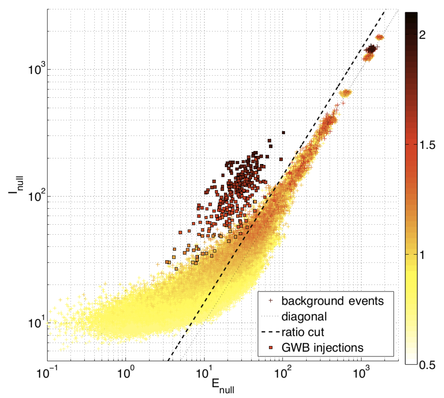
Figure 1: $I_{\textnormal{null}}$ vs. $E_{\textnormal{null}}$ for background events ($+$) and simulated gravitational wave bursts ($\Box$) for a sample GRB search. The colour of the symbols represents the significance associated with each event, with redder (darker) colours representing higher significance. The dotted line shows the $I=E$ diagonal. The dashed line shows the threshold selected by X-Pipeline to separate background and signal; all events that fall below this line are discarded Sutton10 .

The thresholds for the background rejection tests are selected to optimise the trade-off between glitch rejection and signal acceptance. Samples of known background events are generated by analysing data with unphysically large ($>1\,$s) relative time shifts applied to the detector data streams. Known signal events are generated by adding simulated GW signals to the data, known as “injections”. The background and injection events are randomly divided into two equal sets, one that is used for training the pipeline and a second that is used for testing performance. For each $(I,E)$ pair the background rejection test is applied to both the background and injection training samples using a range of trial thresholds. The cumulative distribution of significance of background events surviving the cuts is computed. We then determine the minimum injection amplitude at which 50% of the injections both survive the cuts and have significance greater than a user-specified fraction of the background (e.g., greater than 99% of the background, for a false alarm probability (FAP) $p\leq 0.01$). The optimum thresholds are then defined as those which yield the lowest minimum injection amplitude at the user-specified FAP (i.e., which make the analysis sensitive to the weakest GW signals at fixed FAP). Finally, unbiased estimates of the background distribution and detectable injection amplitudes are made by processing the training data set with our fixed optimal test thresholds.

III Multivariate analysis

The sensitivity of GW transient searches is limited by the ability to distinguish between signals and background. As described above, the standard X-Pipeline analysis uses a simple pass/fail cut in one or more two-dimensional parameter spaces. These cuts only discriminate between signal and background using a few of the variables associated with each event, and ignore other information such as duration, bandwidth, and time-frequency volume. MVA techniques can mine the full parameter space of the events to better discriminate between signal and background. Here we explore the efficacy of MVA in GW detection by using the BDT classifier to re-evaluate the significance of events from an X-Pipeline analysis. We find that the BDT classification of events renders the $(I,E)$ test redundant, and that BDT improves the amplitude sensitivity of the analysis by up to 50% in some cases.

III.1 Toolkit for multivariate analysis

We use the ROOT ROOT:2006vu based software package TMVA Hoecker:2007tp which was developed by the particle physics community. TMVA takes as input known signal and background events. These events are split randomly into two sets, one for training the classifier and the other for testing its performance. This split ensures that the testing produces an unbiased estimate of the classifier performance, since the event used for testing are independent of those used for training.

The results from the training of the classifier are stored in a “weight” file, that contains all the information needed to evaluate the classifier function for any input event and assign a MVA significance value. This significance is a measure of the likelihood of an event being a signal; events with high values of significance are more likely to be signals, and events with small values of significance are more likely to be background. The TMVA package provides many classifiers such as boosted decision trees (BDTs), neural networks (NNs)and projective likelihood Hoecker:2007tp . Initial tests found that a number of the classifiers produced similar results, and that by tuning the classifier parameters an improvement of $\sim 10\%$ was possible; for simplicity we selected BDT using the default parameters for in-depth testing as it exhibited the best performance in the shortest processing time. However, a more in-depth study should be performed to optimise MVA performance for GW applications.

III.2 Boosted Decision Trees

A decision tree consists of a series of yes/no decisions applied to each event, as shown schematically in Fig. 2. Beginning at the root node, an initial criterion for splitting the full set of events is determined. The split criterion consists of a threshold applied to a single variable, selected to best discriminate signal from background. This split results in two branches, each containing a subset of the events. The process then repeats, with a new split criterion being determined at each branch node to further separate signal from background. The splitting process ends once a minimum number of events has been reached within a node, which then becomes a leaf node. We use the default value in TMVA of 400 events. Leaf nodes are labelled as either signal or background depending on the class of the majority of training events that fall within it. The user can specify criteria at which the tree stops being grown, such as how many layers a tree can contain and the total number of nodes which may be created.

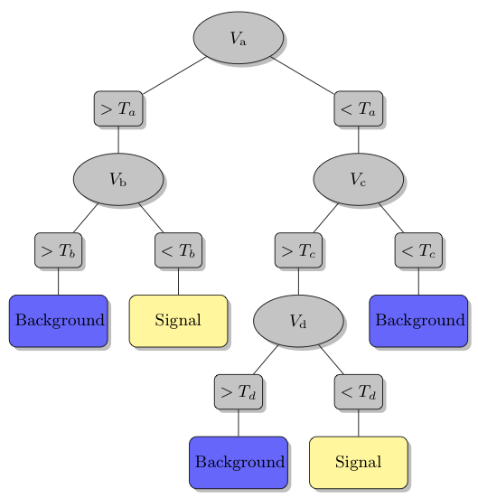
Figure 2: Schematic of a decision tree. Decision nodes for each event variable ($V_{\textnormal{a}}$, $V_{\textnormal{b}}$, $V_{\textnormal{c}}$, and $V_{\textnormal{d}}$) are grey ellipses, with thresholds ($T_{\textnormal{a}}$, $T_{\textnormal{b}}$, $T_{\textnormal{c}}$, and $T_{\textnormal{d}}$) for each branch given in grey rectangles. The events are classified by a majority vote of events in a leaf node as either signal (yellow/ light grey rectangles) or background (blue /dark grey rectangles).

Decision trees are susceptible to statistical fluctuations within the set of training events used to derive the tree structure. To avoid over training, a whole “forest” of decision trees are created, each generated using a randomly selected subset of the training events. The final classification of events is determined by a majority vote from the classifications of each individual tree within the forest. This procedure stabilises the response of individual trees and enhances overall performance. We use the default forest in TMVA made of 400 BDTs.

Another procedure to statistically stabilise the classifier is “boosting”. During training, signal and background events which are misclassified by one tree are given increased weight when constructing the next tree in the forest. We use the default boosting method in TMVA, “AdaBoost”.

IV Signal population

We test BDT for a common GW scenario: the search for a GW burst associated with a GRB.

GRBs are astrophysical events that are observed as an intense flash of gamma rays. Short-duration ($<2\,$s) GRBs are thought to be due to the merger of compact binaries consisting of two neutron stars or a neutron star and a black hole Duncan:1992hh ; NAKAR:2007es . Long-duration ($>2\,$s) GRBs are associated with the core collapse of massive stars Hjorth11 . Both of these progenitor models are highly relativistic and lead to the formation of an accreting black hole (or possibly a magnetar 2009ApJ…702.1171C ). While the GWs produced by the inspiral phase of compact binaries coalescences in short GRBs are well modelled, the expected signal from long GRBs is speculative. A number of such searches for GWs associated with GRBs have been performed by the LIGO and Virgo collaborations Abbott05 ; GRB070201 ; burstGrbS234 ; Acernese08 ; 2010ApJ…715.1453A , including several using X-Pipeline burstGrbS5 ; grb051103 ; Abadie:2012cf .

For our purposes, the GRB trigger provides a known sky position (accurate to within a few degrees) and approximate arrival time (to within a few minutes) of the GW signal, as well as motivating some possible signal models. Furthermore, in each model the GWs are emitted by a quadrupolar mass distribution rotating around the GRB jet axis. Since the GRB is observed at Earth, this implies the observer is near the system axis, which yields circularly polarized GWs Kobayashi:2002ez .

For training and testing the MVA classifier we need to choose a set of simulated GW waveforms to generate our signal data set. Since the expected GW emission is not known with certainty (particularly for long GRBs), we must be careful to avoid training the classifier to find only the waveforms that have been used for training. To do this we use a combination of different waveform classes, which are described below.

circular sine-Gaussians (CSGs):

circular sine-Gaussians (CSGs) are circularly polarized, Gaussian-modulated sinusoids with a fixed central frequency and quality factor (number of cycles); see Fig. 3(a). This simple ad hoc waveform is a standard choice for evaluating the sensitivity of burst searches, and is a special case of the chirplets, which are described below.

binary neutron star inspirals (BNS):

The binary neutron star progenitor model for short GRBs implies an associated “chirp” signal in GWs which can be accurately modelled using a Post-Newtonian expansion Blanchet96 . See Fig. 3 for an example. Since the X-Pipeline analysis is not sensitive to the precise morphology, we use the approximation that is quadrupolar in amplitude and 2 PN in phase and frequency, and cut off the inspiral at the earlier of the coalescence time or the time that the phase second derivative becomes negative.

chirplets:

Chirplets are a generalisation of the CSG waveforms with a non-zero chirp parameter that causes the instantaneous frequency to increase or decrease linearly with time. See Fig. 3(c) for an example.

white noise bursts (WNBs):

White noise bursts are stochastic signals – bursts of Gaussian noise which are white over a frequency band $[f_{\textnormal{low}},f_{\textnormal{low}}+\delta f]$ and which have a Gaussian time profile with decay time $\tau$. See Fig. 3(d) for an example.

The incident sky position is distributed over the GRB sky uncertainty region following a Fisher distribution Was:2012ey . The signal arrival time is distributed uniformly over the interval [$t_{\textnormal{GRB}}-120\,$s, $t_{\textnormal{GRB}}+60\,$s], known as the on-source window. Here $t_{\textnormal{GRB}}$ is the time of the GRB trigger; this on-source window is wide enough to encompass most plausible scenarios of GW emission associated with GRBs. The polarisation angle is uniformly distributed over [0,$\pi$]. For the CSGs and chirplets, the central frequency is distributed uniformly over the search band, 64 Hz to 500 Hz, which is the most sensitive frequency band of the LIGO and Virgo detectors. The signal decay rate $\tau$ is uniformly distributed between the minimum ($1/4$ s) and maximum ($1/128$ s) time resolutions searched by X-Pipeline. The chirp parameter is distributed uniformly between the values which half or double the central frequency in the time interval from $-\tau$ to $\tau$ about the peak time. The binary neutron star inspiral (BNS) signals use a fixed mass of $1.35\,M_{\odot}$ for each of the components of the binary, and an inclination angle between $0^{\circ}$ and $30^{\circ}$. The White noise burst (WNB) waveforms are constructed with fixed values $f_{\textnormal{low}}=50\,\mathrm{Hz}$, $\delta f=100\,\mathrm{Hz}$ and decay time $\tau=0.1\,\mathrm{s}$.

The BNS waveforms are physically motivated signal models. While the other waveforms are ad hoc, the CSGs are a standard waveform class for evaluating the sensitivity of gravitational-wave burst (GWB) searches. Therefore we choose to use a combination of BNS and CSG waveforms for our default training signal set. The WNB and chirplet (chirplet) waveforms are used to test the robustness of the analysis, as described in Section V.6. In particular, the WNB model, being stochastic, provides a rigorous test of the ability of MVA to detect signals of a priori unknown shape.

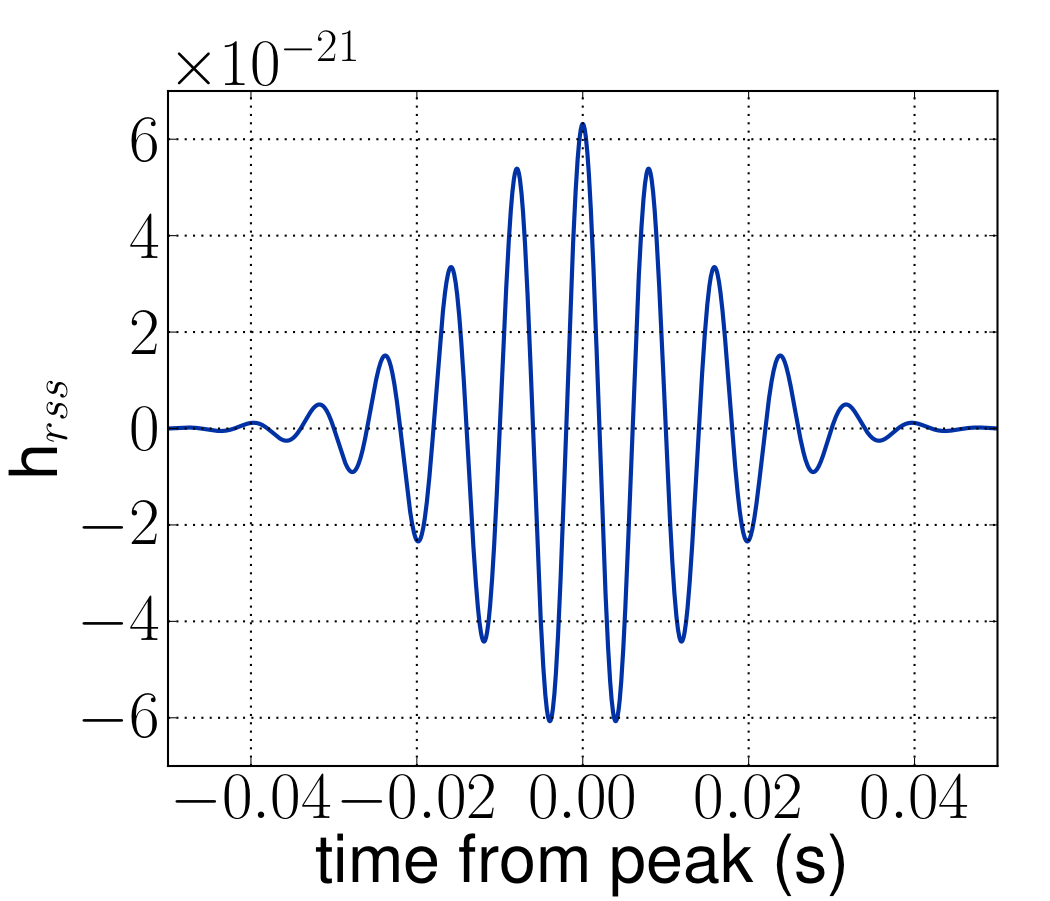
(a)  CSG

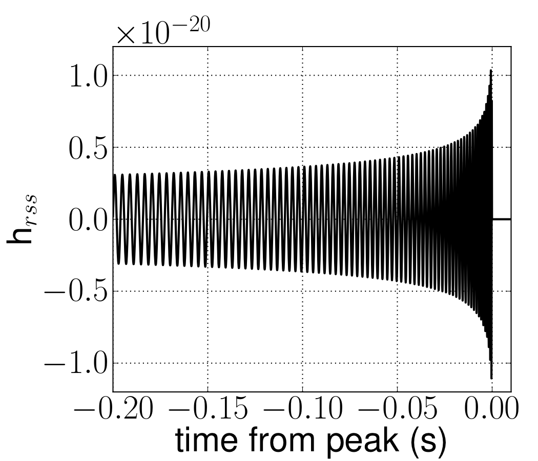
(b)  inspiral

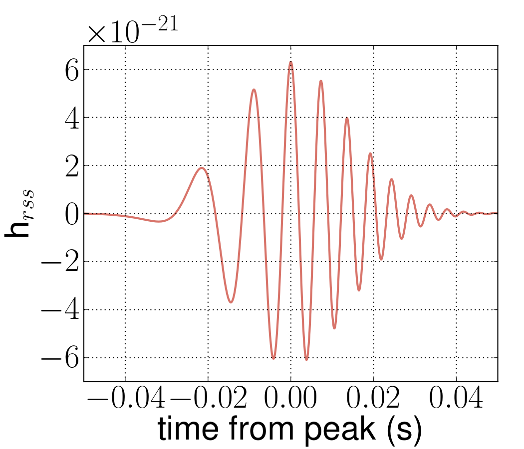
(c)  chirplet

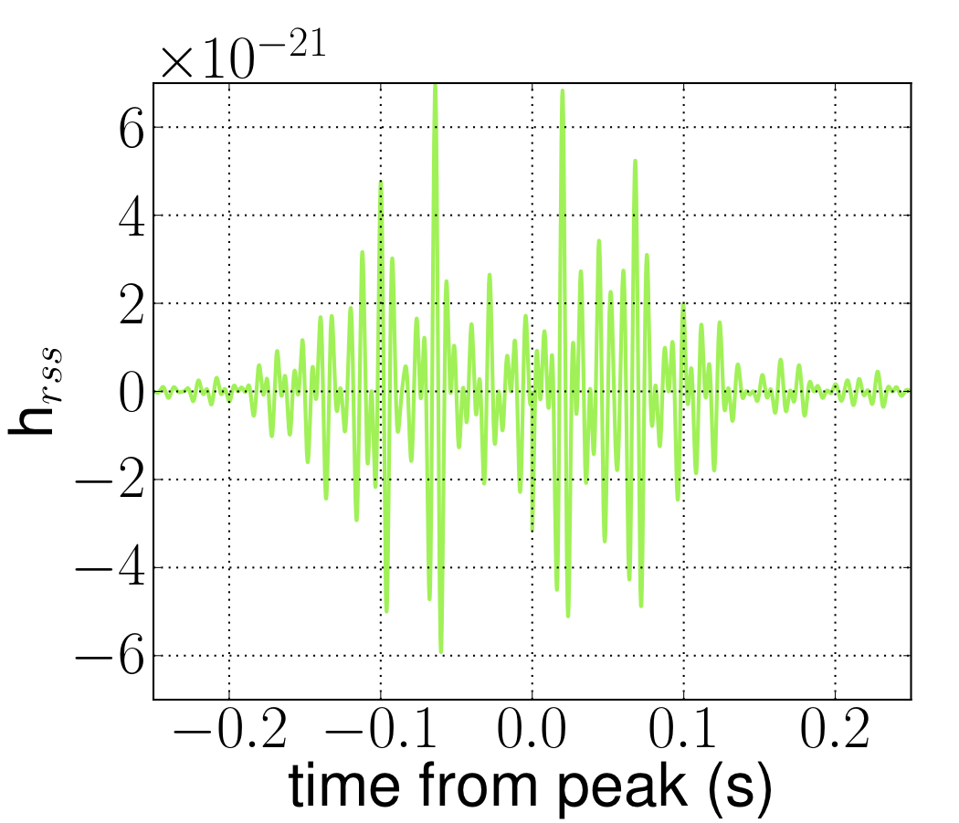
(d)  WNB

Figure 3: Time series of waveforms used for signal injections. For clarity, only one of the two polarisations is plotted.

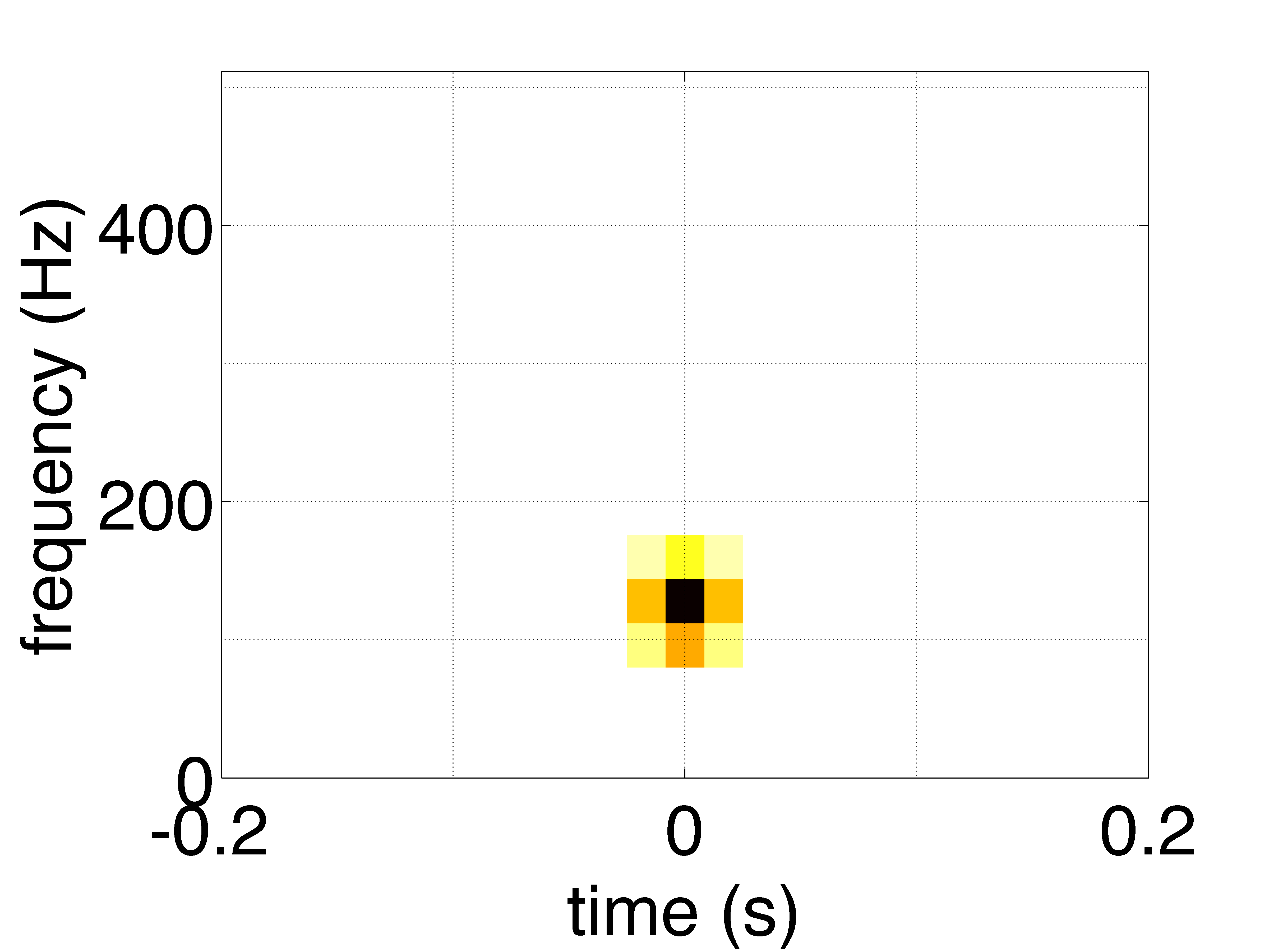
(a)  CSG

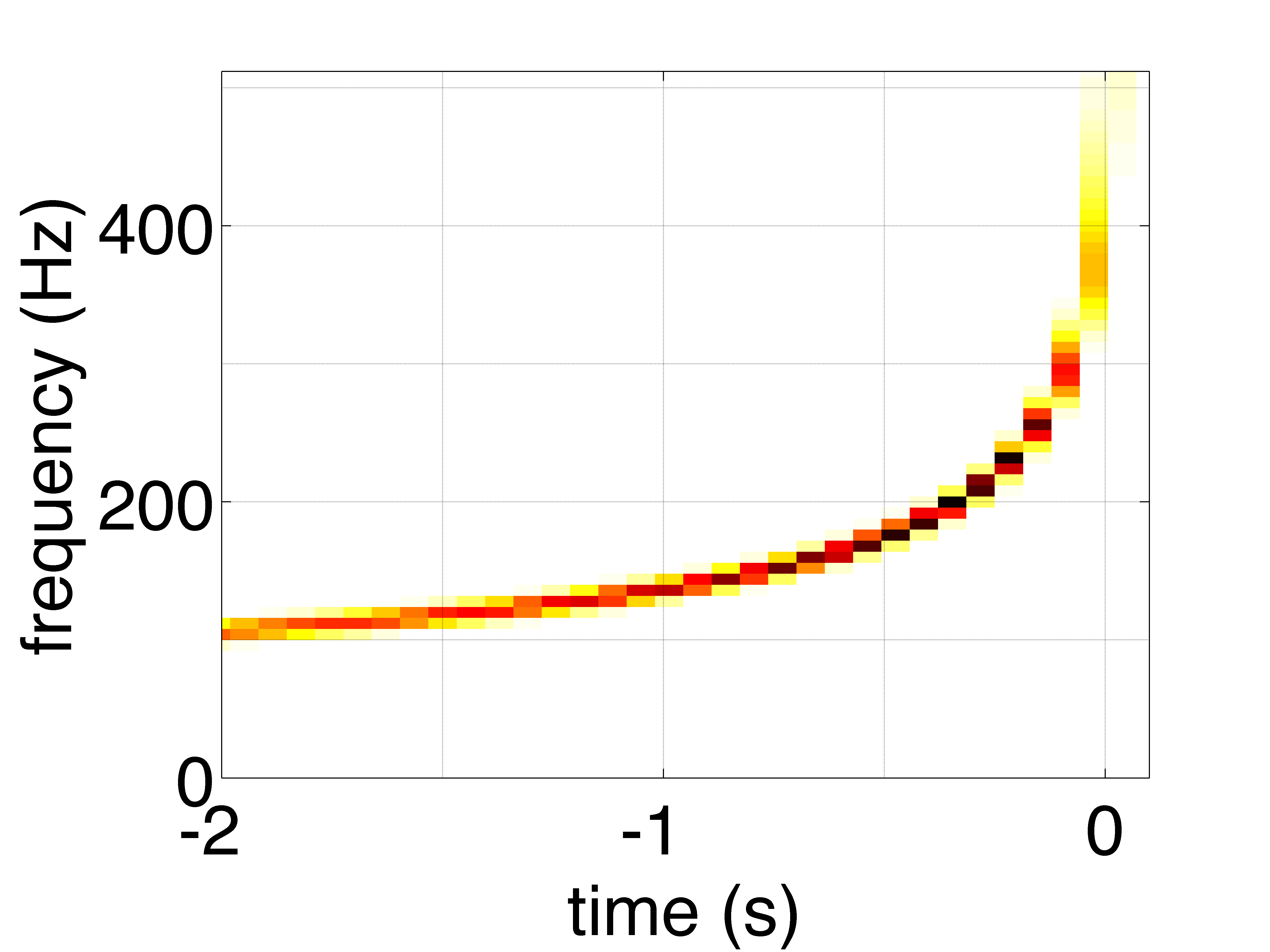
(b)  inspiral

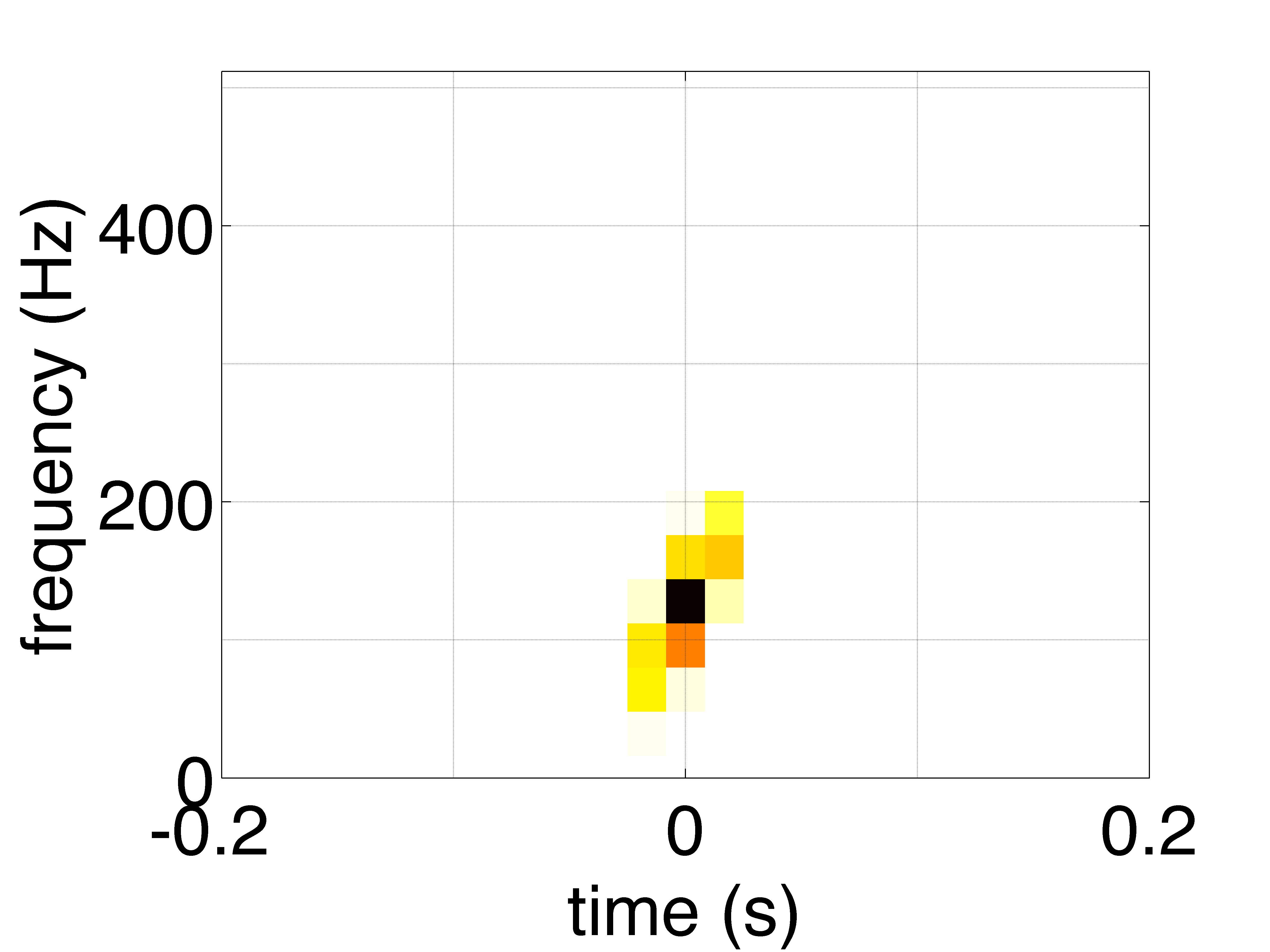
(c)  chirplet

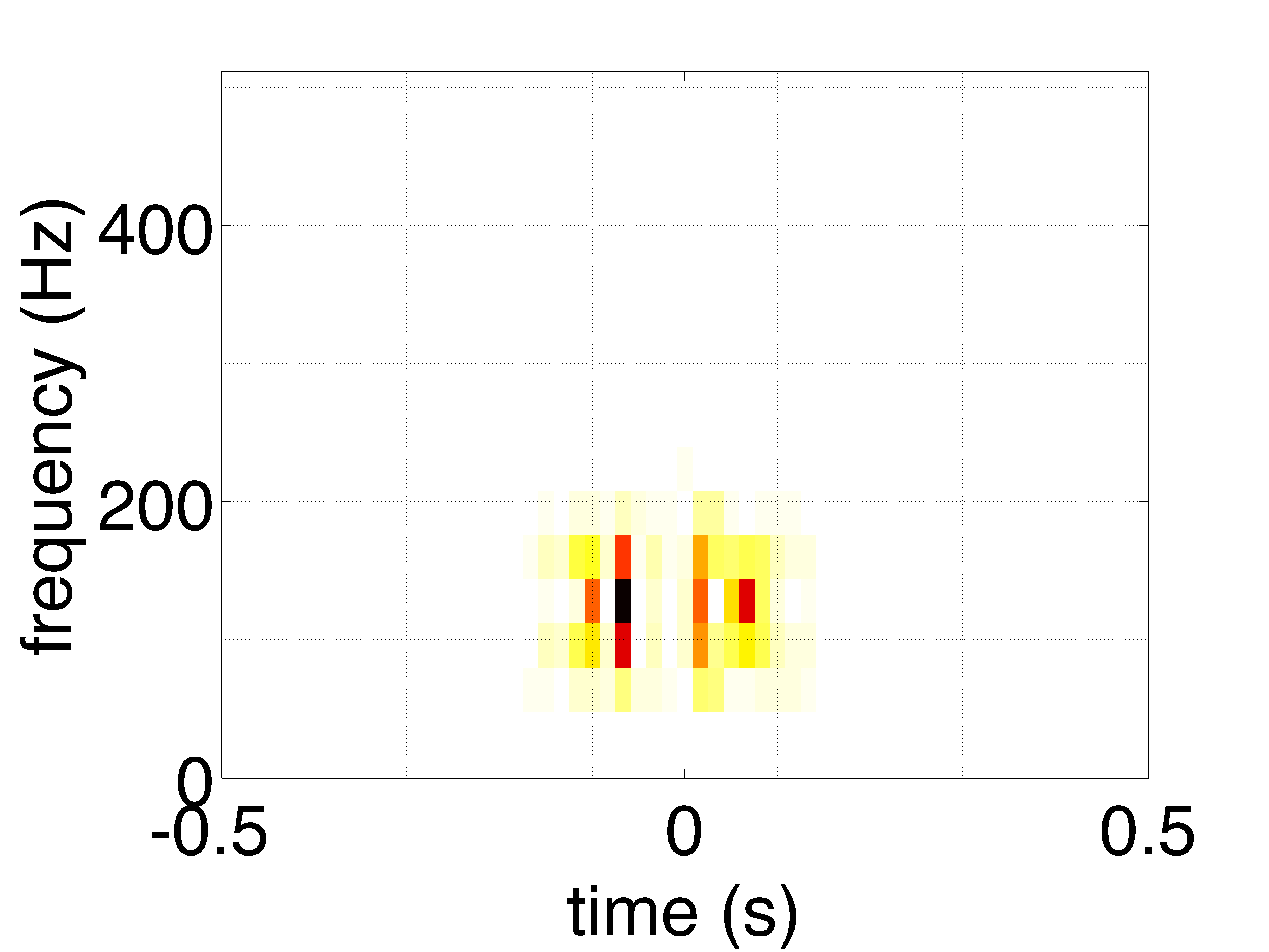
(d)  WNB

Figure 4: Time-frequency spectrograms of waveforms used for signal injections. For clarity, only one of the two polarisations is plotted.

V MVA Performance

We test the efficacy of MVA for GW burst detection by performing a standard analysis of the type used to search for GWs from GRBs. First, X-Pipeline is used to process the data around the time and sky position of a (simulated) GRB trigger. The sensitivity of the analysis is characterised by the minimum amplitude at which at least 50% of simulated signals survive the analysis cuts and have $p$ values of 1% or less, as discussed in Section II. This amplitude is denoted by $h_{\textnormal{rss}}^{50\%}$. The BDT classifier is then applied to the events recorded by X-Pipeline to re-evaluate the significance of each event. The procedure of cut threshold tuning and sensitivity estimation is then repeated using the BDT measure of significance to rank events. The relative performance is measured as the ratio of $h_{\textnormal{rss}}^{50\%}$ for the standard X-Pipeline analysis and the BDT analysis. A ratio greater than unity indicates that the BDT analysis is more sensitive to a particular waveform type than the standard X-Pipeline analysis.

To verify that the performance improvement of MVA is robust, we repeat the GRB analysis for a number of different scenarios. Specifically, we test different GRB sky positions covering a range of network sensitivities, and both large and small sky position uncertainty regions. We also repeat the analysis for a period of particularly poor data quality, and using simulated Gaussian noise to approximate ideal data quality. We find that the relative improvement of BDT to X-Pipeline is consistent across all of these scenarios. We also explore the effect of training using only two types of waveform (CSGs, BNSs) or all four types of waveform. We find that even when searching for signal types that are not included in the training set, the BDT analysis is consistently at least as sensitive as the X-Pipeline analysis, and typically more sensitive. Furthermore, in all cases we find that after processing events with BDT, the X-Pipeline background rejection tests do not improve the sensitivity further; i.e., the BDT has effectively incorporated the signal/background discrimination power of the X-Pipeline background rejection test. Since the test typically requires some assumption about the signal polarisation (in this study we assume circular polarisation), the replacement of the test by BDT actually broadens the range of signals to which the analysis is sensitive.

The following subsections describe each of these tests in turn. We give a full table of the $h_{\textnormal{rss}}^{50\%}$ results for all analyses and all waveforms in Table 3.

Test name	UTC time	Right ascension	Declination	Sky position uncertainty
GRB 060223A (default)	2006-02-23 06:04:23	$55.19^{\circ}$	$-17.13^{\circ}$	$0.03^{\circ}$
sky position 1	2006-02-23 06:04:23	$299.56^{\circ}$	$44.16^{\circ}$	$0.03^{\circ}$
sky position 2	2006-02-23 06:04:23	$311.02^{\circ}$	$32.70^{\circ}$	$0.03^{\circ}$
sky position 3	2006-02-23 06:04:23	$345.40^{\circ}$	$-1.67^{\circ}$	$0.03^{\circ}$
sky position 4	2006-02-23 06:04:23	$31.23^{\circ}$	$-47.51^{\circ}$	$0.03^{\circ}$
large sky position uncertainty 1	2006-02-23 06:04:23	$345.40^{\circ}$	$-1.67^{\circ}$	$9.0^{\circ}$
large sky position uncertainty 2	2006-02-23 06:04:23	$31.23^{\circ}$	$-47.51^{\circ}$	$9.0^{\circ}$
highly non-Gaussian background	2007-06-20 03:05:40	$319.52^{\circ}$	$-57.67^{\circ}$	$0.03^{\circ}$
detection challenge	2007-09-22 03:05:40	$33.44^{\circ}$	$16.94^{\circ}$	$0.03^{\circ}$

Table 2: Trigger parameters used during test analyses. The waveform robustness and Gaussian noise tests used the default GRB 060223A parameters.

V.1 GRB 060223A analysis

For our baseline test we perform an analysis using the parameters (time, sky position) of GRB 060223A, as given in Table 2. GRB 060223A was detected by the Swift satellite (swift04, ) during a period of operation of the LIGO H1, LIGO L1, and Virgo V1 detectors, and localised by Swift to a well-defined sky position. We generate signal events by adding simulated CSG and BNS signals to the three minute on-source window $t_{\textnormal{GRB}}-120\,$s, $t_{\textnormal{GRB}}+60\,$s around the GRB. We generate background events by analysing a three-hour off-source window surrounding the GRB time. These events were split randomly into two sets for training and testing the BDT.

As can be seen in Fig. 5, for CSG signals the BDT analysis gives a substantial improvement in sensitivity – of order $50\%$ – over the standard X-Pipeline analysis. However, there is no significant improvement in the sensitivity to BNS signals (differences of order 5% are not statistically significant).

V.2 Sky position

To verify that the results of the BDT–X-Pipeline comparison are robust, we repeat the test for a variety of other cases. First, we vary the sky position of the GRB trigger. We test four additional sky positions, as listed in Table 2. These positions were chosen to cover a range of different relative detector network sensitivities Was:2012ey .

As can be seen in Fig. 5, for CSG waveforms the BDT analysis gives a consistent improvement in sensitivity of $30-50\%$, for all tested sky positions, compared to the standard X-Pipeline analysis. Again there is no significant change in the sensitivity to BNS signals.

V.3 Large sky position uncertainty

The previous tests have assumed the GRB sky position to be known to high accuracy ($\ll 1^{\circ}$). By contrast, GRBs detected by the GBM instrument on the Fermi satellite have relatively large sky location systematic uncertainties of a few degrees Briggs09 and statistical errors of up to $\sim$10 degrees. This requires analysing the GW data over a grid of trial sky positions covering the error region Was:2012ey . We test the performance of the BDT analysis in this scenario using two different sky positions with sky position uncertainties of $\approx 9^{\circ}$ (see Table 2), which is typical for Fermi-GBM GRBs Meegan:2009qu .

As can be seen in Fig. 5, the BDT performance is consistent with previous tests: for CSG waveforms BDT improves the sensitivity by $40-50\%$, with no significant change in the sensitivity to BNS signals.

V.4 Highly non-Gaussian (glitchy) background

Excess power noise transients can be introduced into the detector data streams by a wide range of known and unknown sources. These glitches are artefacts of the detectors and can be difficult to distinguish from real weak signals. To test the performance of the BDT analysis, we analyse a trigger which is at a time of unusually poor data quality.

As can be seen in Fig. 5, for CSG waveforms the BDT analysis again gives a $\sim$30% improvement in sensitivity, with no notable change for BNS signals compared to the standard X-Pipeline analysis.

V.5 Gaussian background

As a best-case scenario, the performance of the BDT analysis was tested using simulated Gaussian noise with a spectral density coloured to match that of the real detector noise at the time of our default GRB 060223A trigger. All other parameters are kept the same as in the default analysis.

As can be seen in Fig. 5, for CSG waveforms the BDT analysis gives an improvement in sensitivity of $40\%$ compared to the standard X-Pipeline analysis. There is no notable change in the sensitivity to BNS signals.

V.6 Waveform robustness

In GW burst searches the signal waveform is usually not known a priori. It is therefore of the utmost importance to verify that MVA is able to detect waveforms with morphologies that differ from those used for training; at the very least, MVA should not have worse sensitivity for unknown waveforms than the standard analysis. We study this issue by repeating our analysis using different waveform sets for training and testing. Specifically, we evaluate the BDT performance for detecting chirplet and WNB waveforms in two cases: one in which the BDT is trained using CSG and BNS signals only (and not chirplet or BNS signals) and again after training on all four waveform types (CSG, BNS, chirplet, WNB). We refer to these as the two-waveform and four-waveform robustness tests.

Fig. 5 shows that in the two-waveform test (training on CSG and BNS only) the BDT analysis shows the same performance for CSG and BNS as was seen in the default GRB 060223A analysis. This is expected, as the tests are identical as far as these waveforms are concerned. However, BDT also gives an improvement in sensitivity of order $50\%$ for chirplet waveforms compared to the standard X-Pipeline analysis. This implies that the CSGs and chirplets are sufficiently similar in terms of a time-frequency analysis that an MVA trained to detect one can detect the other. More surprising is the BDT performance for WNBs. These waveforms are not detectable by the standard X-Pipeline analysis. This happens because the two GW polarisations are uncorrelated for a WNB, whereas the X-Pipeline background rejection test applied to the signal stream (discussed in Section II) assumes the two polarisations are related by $90^{\circ}$ phase shift, as expected for a circularly polarised signal. The BDT analysis is able to recover these waveforms, albeit with an $h_{\mathrm{rss}}^{50\%}$ value about twice as high as for the case of training with WNBs (discussed below).

The four waveform robustness test used independent samples of all four waveform types (CSG, BNS, chirplet, and WNB) for both training and testing. From Fig. 5 we again see the same performance from BDT for the CSG and BNS signals. However, with training extended to include chirplet and WNB waveforms, we see slightly less improvement of sensitivity to chirplets (only $30\%$ compared to the standard X-Pipeline analysis). This is partly due to a small improvement in the sensitivity of the X-Pipeline analysis to chirplets when they are included in the training. However, most of the change is due to a decrease in sensitivity of the BDT analysis ($\sim$ 15% drop) from the two-waveform case; we attribute this to the inclusion of WNBs in the training. The classifier in this case finds a compromise between the sensitivity to circularly polarised signals and unpolarised signals in the training. This can be seen as the sensitivity to WNBs is dramatically improved, by more than a factor of two compared to the two-waveform BDT analysis. The standard X-Pipeline analysis can also detect WNBs when trained with all four waveform types; in this case the automated background rejection tuning places less emphasis on the tests that assume circular polarisation and more on the polarisation-independent null stream test. We find a net sensitivity improvement of $\sim\,15\%$ by BDT relative to X-Pipeline for WNBs when training includes these waveforms.

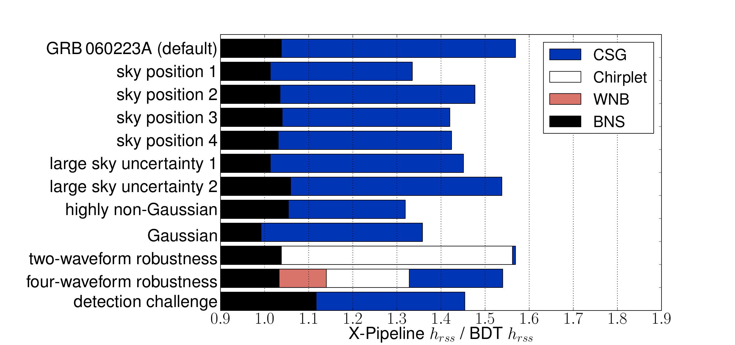
Figure 5: Ratio of the minimum-detectable signal amplitudes $h_{\mathrm{rss}}^{50\%}$ for the standard X-Pipeline analysis and the BDT analysis for each of the signal waveforms and scenarios described in Section V. Ratios greater than 1 indicate the BDT analysis is more sensitive than the standard X-Pipeline analysis. (Equivalently, for a fixed signal amplitude the distance reach of the BDT search is greater than that of the X-Pipeline search by this ratio.) CSG performance is given in blue (dark grey), BNS performance is given in black, chirplet performance is given in white, and WNB performance is given in red (light grey). The standard X-Pipeline analysis is unable to recover WNB signals in the robustness two-waveform test, so the sensitivity ratio is ill-defined in this case. All $h_{\mathrm{rss}}^{50\%}$ values of results can be found in Table 3.

V.7 Detection challenge case

Analysis	waveform	X-Pipeline $h_{\textnormal{rss}}^{50\%}$	BDT $h_{\textnormal{rss}}^{50\%}$	ratio
GRB 060223A	CSG	$4.90\times 10^{-22}$	$3.12\times 10^{-22}$	$1.569$
	BNS	$1.09\times 10^{-21}$	$1.05\times 10^{-21}$	$1.038$
sky position 1	CSG	$8.70\times 10^{-22}$	$6.51\times 10^{-22}$	$1.335$
	BNS	$2.05\times 10^{-21}$	$2.02\times 10^{-21}$	$1.013$
sky position 2	CSG	$6.43\times 10^{-22}$	$4.36\times 10^{-22}$	$1.477$
	BNS	$1.42\times 10^{-21}$	$1.37\times 10^{-21}$	$1.035$
sky position 3	CSG	$4.07\times 10^{-22}$	$2.86\times 10^{-22}$	$1.420$
	BNS	$9.08\times 10^{-22}$	$8.73\times 10^{-22}$	$1.040$
sky position 4	CSG	$3.91\times 10^{-22}$	$2.74\times 10^{-22}$	$1.424$
	BNS	$9.03\times 10^{-22}$	$8.76\times 10^{-22}$	$1.031$
large sky position uncertainty 1	CSG	$4.19\times 10^{-22}$	$2.89\times 10^{-22}$	$1.451$
	BNS	$9.39\times 10^{-22}$	$9.26\times 10^{-22}$	$1.013$
large sky position uncertainty 2	CSG	$4.04\times 10^{-22}$	$2.63\times 10^{-22}$	$1.538$
	BNS	$9.21\times 10^{-22}$	$8.70\times 10^{-22}$	$1.059$
highly non-Gaussian background	CSG	$5.70\times 10^{-22}$	$4.32\times 10^{-22}$	$1.319$
	BNS	$1.38\times 10^{-21}$	$1.31\times 10^{-21}$	$1.054$
Gaussian background	CSG	$4.48\times 10^{-22}$	$3.30\times 10^{-22}$	$1.358$
	BNS	$1.01\times 10^{-21}$	$1.02\times 10^{-21}$	$0.992$
two-waveform robustness	CSG	$4.90\times 10^{-22}$	$3.12\times 10^{-22}$	$1.569$
	BNS	$1.09\times 10^{-21}$	$1.05\times 10^{-21}$	$1.038$
	chirplet	$5.03\times 10^{-21}$	$3.22\times 10^{-22}$	$1.562$
	WNB	nan	$1.65\times 10^{-21}$	nan
four-waveform robustness	CSG	$4.91\times 10^{-22}$	$3.19\times 10^{-22}$	$1.540$
	BNS	$1.10\times 10^{-21}$	$1.06\times 10^{-21}$	$1.033$
	chirplet	$4.81\times 10^{-22}$	$3.62\times 10^{-22}$	$1.328$
	WNB	$7.45\times 10^{-22}$	$6.54\times 10^{-22}$	$1.140$
detection challenge case	CSG	$4.92\times 10^{-22}$	$3.38\times 10^{-22}$	$1.454$
	BNS	$7.65\times 10^{-22}$	$6.85\times 10^{-22}$	$1.117$

Table 3: Sensitivity of the standard X-Pipeline and BDT-augmented analyses for each test scenario and waveform type. $h_{\textnormal{rss}}^{50\%}$ (Hz^-1/2) is the minimum amplitude for which at least 50% of simulated signals survive the analysis cuts and have FAP of 1% or less. The last column is the ratio of $h_{\textnormal{rss}}^{50\%}$ for X-Pipeline and BDT; values greater than unity indicate that BDT is more sensitive. Equivalently, for a fixed signal amplitude the distance reach of the BDT search is greater than that of the X-Pipeline search by this ratio.

Recent science runs of the LIGO and Virgo detectors have included a “blind injection challenge” wherein a small number of simulated signals are secretly added to the data via the interferometer control systems lowMassS5y2 ; 2010ApJ…715.1453A ; Abadie:2012cf ; lowMassS6 . These signals are used to test the analysis procedures. Our final MVA test is to analyse one of these signals, to demonstrate that the improvement in sensitivity extends to false-alarm rates low enough to permit a detection claim at the $3\sigma$ level.

For this test we select the “equinox event”, an injection performed on 22 September 2007. The simulated waveform was approximately a single-cycle sine-Gaussian with a central frequency of approximately 60 Hz and an amplitude of $h_{\mathrm{rss}}=1.0\times 10^{-21}\mathrm{Hz}^{-1/2}$; see Fig. 6. The relative amplitudes of the plus and cross polarisations were consistent with an inclination angle of approximately $30^{\circ}$. The sky position is shown in Table 2.

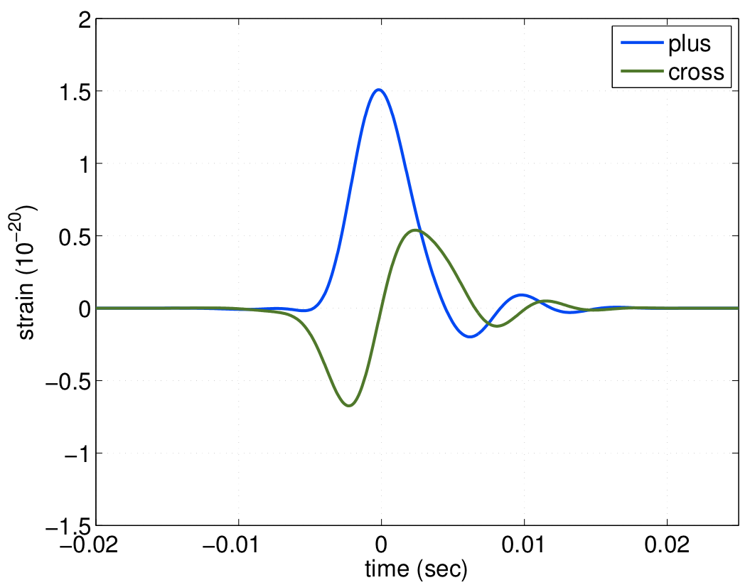
Figure 6: Time series of the “equinox event” signal in the detection challenge test.

We analysed this injection using the standard GRB procedure; i.e., assuming the sky position and approximate time of the event were known a priori due to observation of an electromagnetic counterpart. In our previous tests we evaluated the minimum detectable signal amplitude at a fixed false alarm probability of 1%. This follows the standard use of X-Pipeline in GRB searches burstGrbS5 ; Abadie:2012cf . However, in order to claim the detection of a gravitational-wave signal, much lower false-alarm probabilities are required. In particular, a $3\sigma$ significance requires a false-alarm probability of $p\leq 0.0027$. Furthermore, a typical search includes 100–150 GRB triggers, which must be accounted for in the trials factor. A $3\sigma$ significance with 150 trials requires $p\lesssim 2\times 10^{-5}$ for an individual event. For this analysis we therefore generate extra background samples and tune the background rejection tests to yield the lowest minimum injection amplitude at a FAP of $p=10^{-5}$. Since the blind injection was not added to the Virgo detector data, we analyse the event using the LIGO H1 and L1 detectors only. All other analysis parameters are the same as for the GRB 060223A test, including training and testing with CSG and BNS waveforms.

Fig. 7 shows the cumulative distribution of the detection statistic for the loudest background event per three minute interval (the on-source interval) returned by the standard X-Pipeline analysis and the BDT analysis. Both distributions are consistent with a power-law relationship between false alarm probability and detection statistic down to the lowest false alarm probabilities measured, $p\simeq 10^{-5}$. From Fig. 5 we can see that the BDT analysis gives an improvement in sensitivity compared to the standard X-Pipeline analysis that is consistent with previous tests. This demonstrates that the benefits of the BDT analysis extend down to false alarm rates sufficient for $3\sigma$ detections in GRB triggered searches.

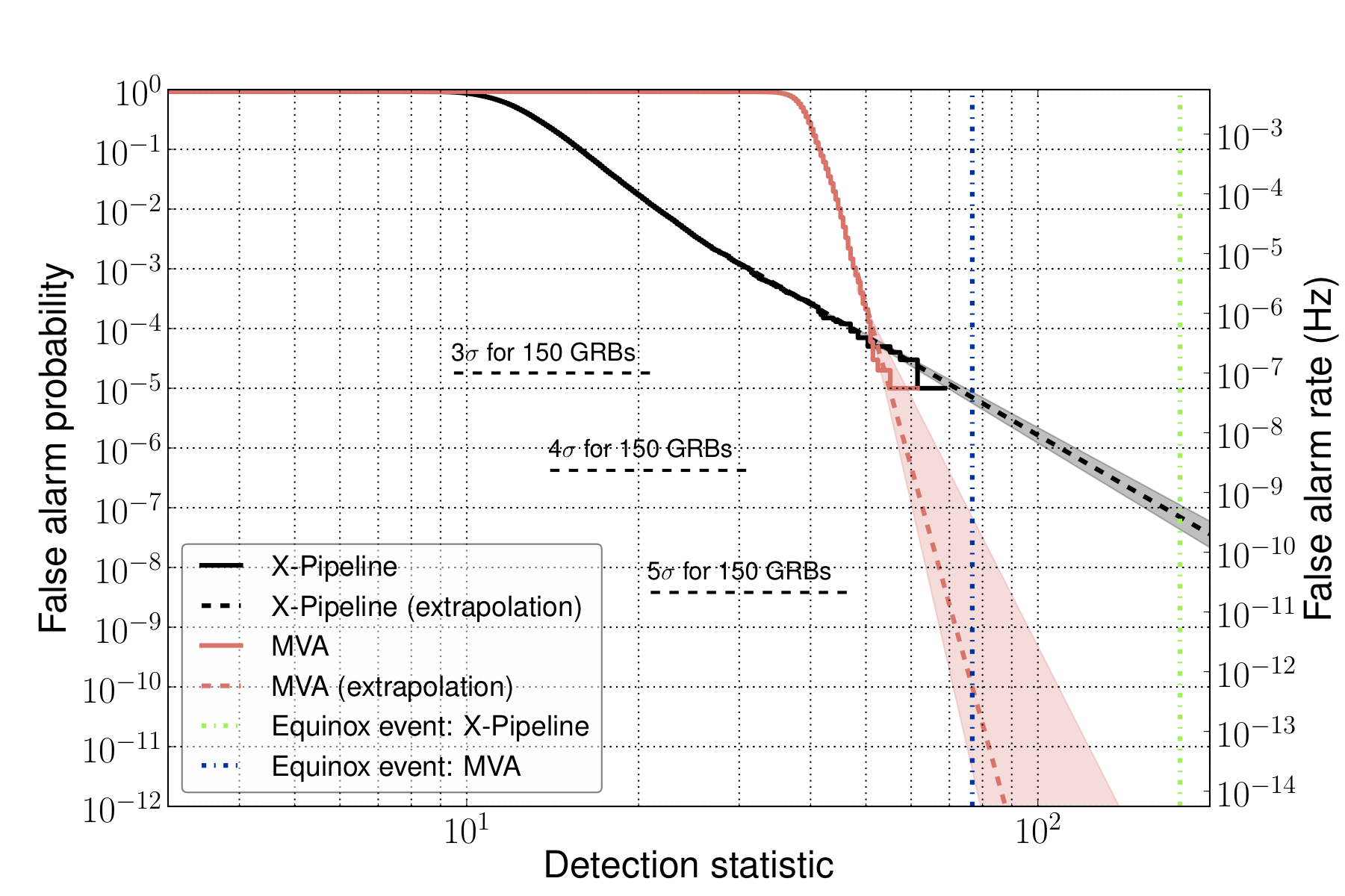
Figure 7: Background distributions for the X-Pipeline and BDT analyses of the equinox event. The background distributions are shown as solid lines. The power-law extrapolations are shown as dashed lines, with the shading indicating the estimated uncertainty in the extrapolations. The value of the detection statistic of the equinox event is shown by the green and blue vertical lines for the X-Pipeline and BDT analyses respectively.

Of particular interest is the significance assigned to the equinox event itself. The vertical lines in Fig. 7 indicate the value of the detection statistic returned by X-Pipeline and BDT. In both analyses the equinox event is clearly detected, with a significance higher than any of the background events. In order to estimate the approximate false alarm probability for the equinox event, we extrapolate the background distributions using a best-fit power law. This yields $p\simeq 7\times 10^{-8}$ ($5.4\sigma$) for the standard X-Pipeline analysis and $p\simeq 1\times 10^{-10}$ ($6.5\sigma$) for the BDT analysis. The shaded bands indicate the plausible extrapolations from using a varied number of data points to determine the best-fit parameters, which can be taken as an estimate of the uncertainty in the extrapolation. While these are estimates, the BDT analysis assigns a false alarm probability which is at worst consistent with the X-Pipeline result, and the range of possible extrapolations suggest that the false alarm probability could be significantly lower.

VI Discussion and Conclusions

The tests shown in Section V and Fig. 5 demonstrate that the BDT-augmented analysis yields a consistent improvement in sensitivity to some signal types at fixed false-alarm rate with respect to the standard X-Pipeline analysis. The improvement holds regardless of the incident direction of the signal or its sky location uncertainty, the data quality, and the network of detectors. Most importantly, the BDT analysis is always at least as sensitive as X-Pipeline, even to signals of different morphology to those used in training, and the sensitivity improvement extends down to false alarm probabilities required for detection.

The degree to which BDT outperforms the standard X-Pipeline analysis depends on the signal waveform. For CSGs, which have compact time-frequency distributions, we find a consistent improvement in sensitivity of $35-55\%$. By contrast, for BNS signals, which are long-duration and have extended time-frequency distributions, the average improvement in sensitivity is only 4%. The BDT analysis also yields improved sensitivity to chirplet and WNB waveforms, regardless of whether they were included in the training set or not. The large increase in sensitivity to chirplet waveforms seen in the two-waveform robustness test is likely due to these waveforms being very similar to the CSGs. The smaller improvement seen in the four-waveform test is likely due to the classifier compromising performance between the mix of waveforms; the effect of this is a decrease in sensitivity gain for both the CSG and chirplet waveforms, but a dramatic improvement in sensitivity to WNB waveforms.

The robustness of the BDT analysis to signals of different morphology from those used in training is crucial, because accurate signal waveforms are not known in most burst searches. (In fact, the WNB results from the two-waveform robustness test show that BDT can actually improve the sensitivity to a priori unknown waveforms by removing the need for X-Pipeline’s polarisation-specific background rejection tests.) The robustness of BDT may be due to the fact that the MVA does not have access to the raw GW data, but rather only to characteristics passed on by X-Pipeline. In particular, the only time-frequency information that is available to BDT are the time and frequency extent of the event, its peak time and frequency, and the number of time-frequency pixels; no shape information is recorded. In principle shape information could be used to improve signal/background discrimination, e.g. by recognising the characteristic chirp shape of inspiral signals (see Fig. 3). However, this would presumably also make the MVA analysis more waveform-specific, and less sensitive to signals not included in the training. Further study of the waveform dependence of MVA analyses is warranted.

Figure 8: Example decision tree used in the GRB 060223A BDT analysis. Decision nodes are grey ellipses, with thresholds for a branch given in grey rectangles. Leaf nodes for signal events are light yellow rectangles and for background events are dark blue rectangles.

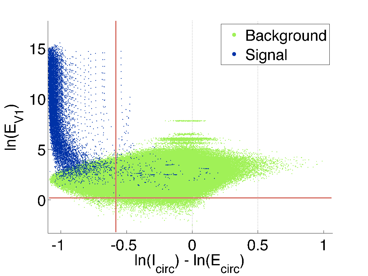
Figure 9: Scatter plot of signal and background events from the GRB 060223A analysis. The red lines indicate the cuts applied by the decision tree shown in Fig. 8.

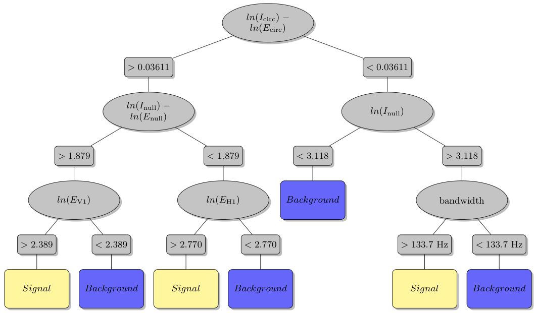
Figure 10: Example decision tree used in the GRB 060223A BDT analysis. Decision nodes are grey ellipses, with thresholds for a branch given in grey rectangles. Leaf nodes for signal events are light yellow rectangles and for background events are dark blue rectangles.

Fig. 8 and Fig. 10 show sample decision trees that were used in the GRB 060223A analysis. Decision nodes for each variable are shown as grey ellipses with the thresholds for a branch shown in grey rectangles. The leaf nodes are light yellow rectangles for signal and dark blue rectangles for background.

We first consider the simple decision tree shown in Fig. 8. In this example the first cut is applied to the difference between the incoherent and coherent energies, $\ln(I_{\textnormal{circ}})-\ln(E_{\textnormal{circ}})$, at a threshold of $-0.581$. Events above this threshold are classified as background, while events below this threshold are then cut on the energy in the Virgo detector, $\ln(E_{\textnormal{V1}})$, which has a threshold of $0.183$. Events above this second threshold are classified as signal, while events below are classified as background. The logic behind these choices can be understood from Fig. 9, which shows a scatter plot of $\ln(E_{\textnormal{V1}})$ vs. $\ln(I_{\textnormal{circ}})-\ln(E_{\textnormal{circ}})$ for the training events. The red lines are the thresholds used in the example decision tree to separate the signal events from the majority of the background events. While this single tree assigns a large fraction of the background events to the signal leaf node (the upper-left rectangle), the final significance of events is determined collectively by 400 such trees, each generated from a random subset of the training data. A more complicated tree is shown in Fig. 10, which classifies events based on 6 of their properties.

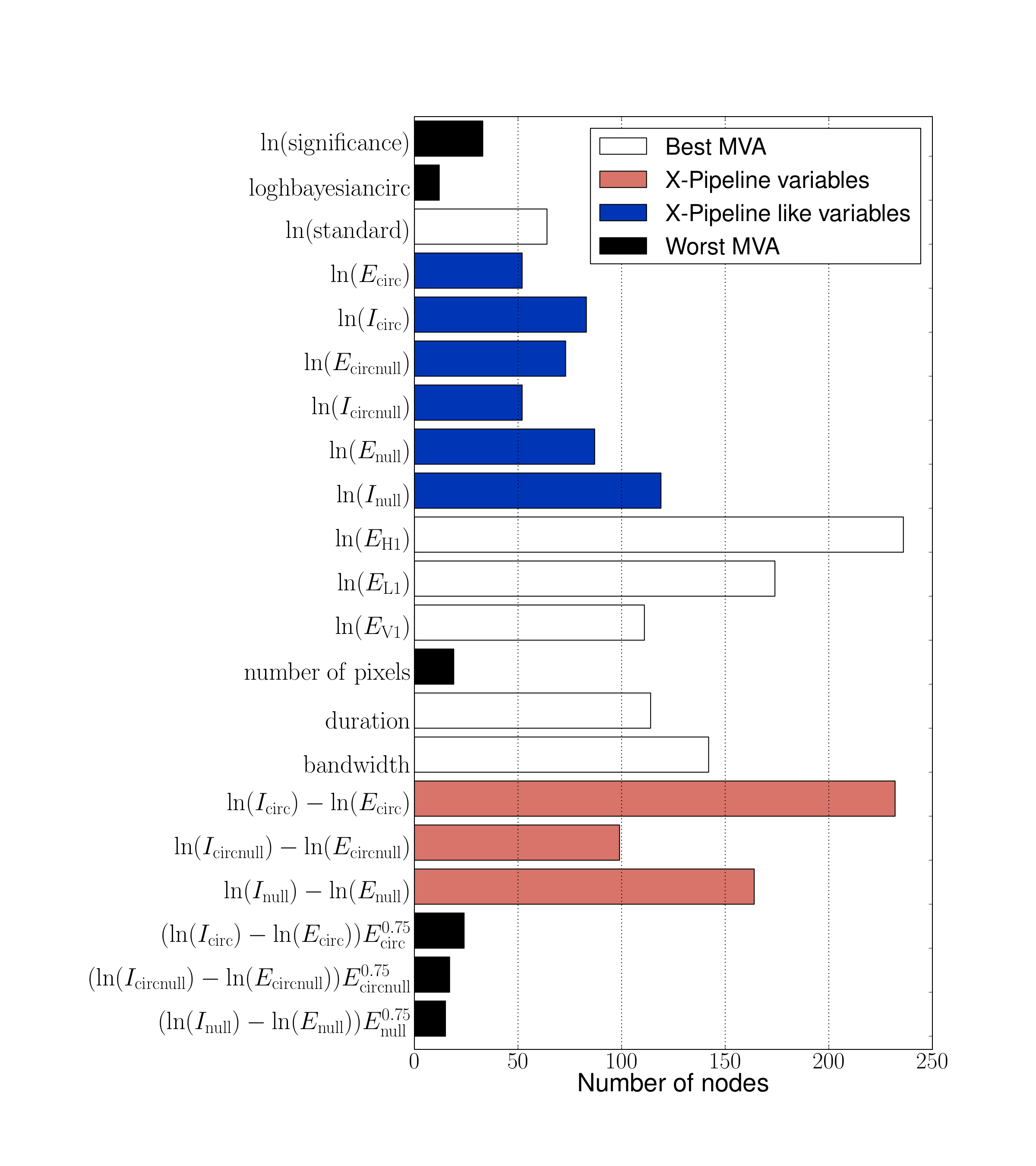
Figure 11: Bar chart of the number of times each variable or variable combination is used at decision tree nodes in the BDT forest for the GRB 060223A analysis. The “X-Pipeline variables” are combinations of variables that precisely match those used used in theX-Pipeline background rejection test of equation (1), while the “X-Pipeline like variables” can be used to construct the cut of equation (2). Together these are among the variables most frequently selected by the BDT analysis, accounting for half of all nodes. The single-detector energies, duration, and bandwidth are selected for 40% of all nodes. These variables are not used by X-Pipeline demonstrating how MVA makes use of the full dimensionality of the data. The remaining variables collectively account for approximately 10% of all nodes. See Tab. 1 for definitions of the variables.

We gain further insight into the performance of the BDT analysis by considering how frequently different event variables are used in the classification. Fig. 11 is a bar chart of the total number of times each variable or combination of variables reported by X-Pipeline is used in one of the decision nodes for the GRB 060223A analysis. We take this as an indicator of the value of each variable for signal/background discrimination. The X-Pipeline background rejection tests are based on combinations of $E_{\mathrm{circ}}$ and $I_{\mathrm{circ}}$, $E_{\mathrm{circnull}}$ and $I_{\mathrm{circnull}}$, and $E_{\mathrm{null}}$ and $I_{\mathrm{null}}$, as given in equations (1) and (2). The pairwise differences $\ln(I)-\ln(E)=\ln(I/E)$ are labeled as “X-Pipeline variables” in the chart, because thresholding on these differences is equivalent to applying the X-Pipeline test of equation (1). We see that these are some of the most frequently used combinations, selected for approximately 26% of all nodes. The individual $\ln(I)$ and $\ln(E)$ variables are labeled as “X-Pipeline like variables” because the remaining X-Pipeline cut of equation (2) can be constructed from them. These are selected for a total of 24% of the nodes. The selection of these variables by BDT for approximately 50% of the nodes affirms their usefulness for signal/background discrimination, as expected from their demonstrated value in X-Pipeline’s background rejection tests. However, close to half of the BDT nodes use variables that are not used by X-Pipeline. This is a clear demonstration of an MVA making use of the full dimensionality of the data. In particular, the single-detector energies are selected for approximately 27% of all nodes. Thresholding on these values is equivalent to thresholding on the event signal-to-noise ratio in the individual detectors Sutton10 , which is not done in X-Pipeline. The event duration and the bandwidth are also useful, selected for 13% of all nodes. The remaining variables collectively account for approximately 10% of all nodes. Interestingly, the number of pixels (time-frequency area of the event) is one of the variables that is not particularly useful for signal/background discrimination.

Another view of the merits of BDT classification is given by Fig. 12. These show scatter plots of $I_{\mathrm{circ}}$ vs. $E_{\mathrm{circ}}$ for testing data from the GRB 060223A analysis. The squares represent simulated CSG events at the amplitude for which the detection efficiency is approximately 90%. Fig. 12(a) shows the events coloured by their significance in the X-Pipeline analysis, as well as the threshold line for the X-Pipeline background rejection test. Event significance increases with $I_{\mathrm{circ}}$ or $E_{\mathrm{circ}}$; i.e., along the diagonal, whereas the signal and background are separated primarily in the orthogonal direction. Signals become detectable when they do not overlap the background distribution in $I_{\mathrm{circ}}$ vs. $E_{\mathrm{circ}}$ space. Fig. 12(b) shows the same background events as ranked by BDT. By contrast with the X-Pipeline analysis, significance increases with distance from the diagonal, so that no additional background rejection test is required. Simulated CSG events are detectable at lower amplitudes, even though they overlap the background distribution in $I_{\mathrm{circ}}$ vs. $E_{\mathrm{circ}}$ space, because the BDT analysis takes account of other event properties such as the single-detector energies.

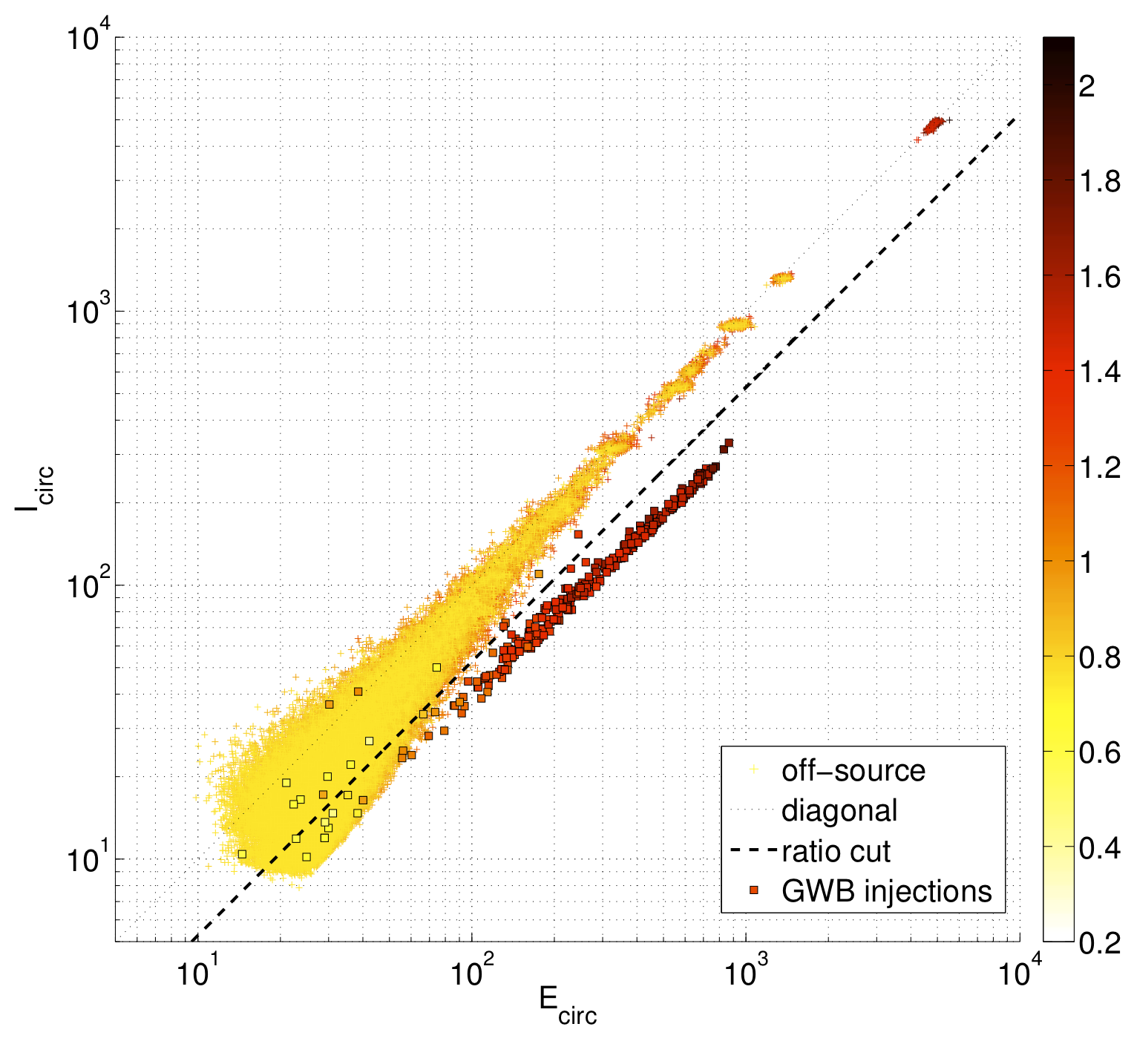
(a) X-Pipeline

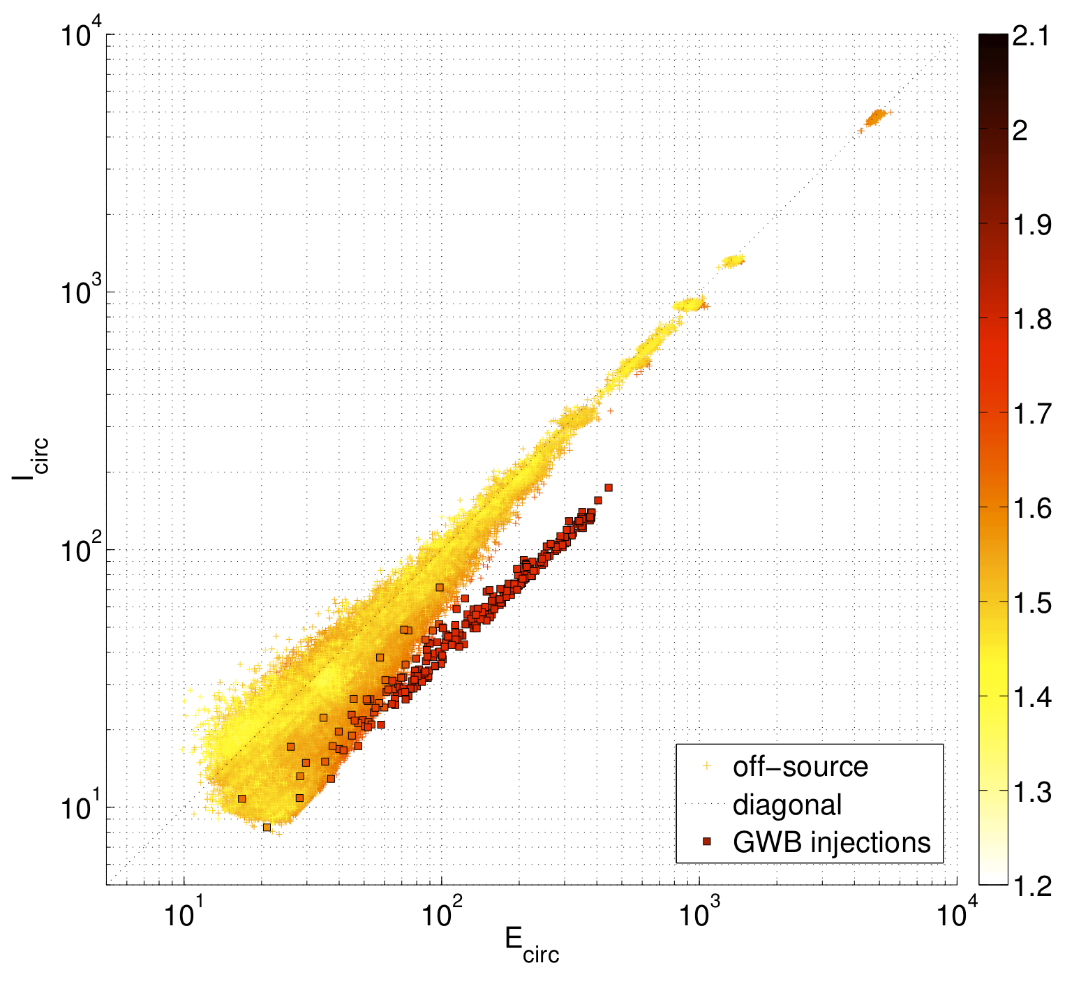
(b) BDT

Figure 12: (a) - Scatter plot of $I_{\mathrm{circ}}$ vs. $E_{\mathrm{circ}}$ for testing data from the GRB 060223A X-Pipeline analysis. The squares represent simulated CSG events at the amplitude for which the X-Pipeline detection efficiency is approximately 90%. Events are coloured by their significance in the X-Pipeline analysis. The dashed line is the threshold line for the X-Pipeline background rejection test; events above this line are discarded. (b) - Scatter plot of $I_{\mathrm{circ}}$ vs. $E_{\mathrm{circ}}$ for testing data from the GRB 060223A BDT analysis. The squares represent simulated CSG events at the amplitude for which the BDT detection efficiency is approximately 90%. Events are coloured by their significance in the BDT analysis.

The results presented here indicate that multivariate analysis techniques may be valuable for improving the sensitivity of searches for unmodelled gravitational-wave bursts. Additional studies are merited, particularly using a wider range of waveform morphologies, larger background samples and lower false alarm rates, and extending to all-sky untriggered searches. We will revisit these questions in future publications.

References

- [1] G. M. Harry. Advanced LIGO: The next generation of gravitational wave detectors. Class.Quant.Grav., 27:084006, 2010.
- [2] The Virgo Collaboration. Advanced virgo baseline design note vir027a0(2009). https://tds.ego-gw.it/itf/tds/file.php?callFile=VIR-0027A-09.pdf.
- [3] K. Somiya for the KAGRA Collaboration. Detector configuration of KAGRA-the Japanese cryogenic gravitational-wave detector. Classical and Quantum Gravity, 29(12):124007, 2012.
- [4] P Mészáros. Gamma-ray bursts. Reports on Progress in Physics, 69(8):2259–2321, August 2006.
- [5] C. D. Ott. The gravitational-wave signature of core-collapse supernovae. Classical and Quantum Gravity, 26(6):063001, March 2009.
- [6] K. Kotake. Multiple physical elements to determine the gravitational-wave signatures of core-collapse supernovae. ArXiv e-prints, October 2011.
- [7] A. Corsi and P. Mészáros. Gamma-ray Burst Afterglow Plateaus and Gravitational Waves: Multi-messenger Signature of a Millisecond Magnetar? Astrophys. J., 702(2):1171–1178, September 2009.
- [8] B. P. Abbott et al. Search for gravitational waves from low mass compact binary coalescence in 186 days of LIGO’s fifth science run. Phys. Rev. D, 80(4):047101, 2009.
- [9] J. Abadie et al. Search for gravitational waves from low mass compact binary coalescence in LIGO’s sixth science run and Virgo’s science runs 2 and 3. Phys. Rev. D, 85(8):82002, April 2012.
- [10] J. Abadie et al. All-sky search for gravitational-wave bursts in the first joint LIGO-GEO-Virgo run. Phys. Rev. D, 81:102001, 2010.
- [11] J. Abadie et al. All-sky search for gravitational-wave bursts in the second joint LIGO-Virgo run. Phys. Rev. D, February 2012.
- [12] B. Allen. 2 time-frequency discriminator for gravitational wave detection. Phys. Rev. D, 71(6):062001, March 2005.
- [13] M. Wa̧s, P. J. Sutton, G. Jones, and I. Leonor. Performance of an externally triggered gravitational-wave burst search. Phys. Rev. D, 86(2):022003, July 2012.
- [14] A. Hoecker et al. TMVA - Toolkit for Multivariate Data Analysis. arXiv.org, March 2007.
- [15] T. Hastie, R. Tibshirani, and J. Friedman. The Elements of Statistical Learning. Springer, 2001.
- [16] A.R. Webb. Feature selection and extraction. John Wiley & Sons Ltd, Chichester, West Sussex, England, 2nd edition, 2002.
- [17] D0 Collaboration. Search for the standard model Higgs boson in tau lepton pair final states. Physics Letters B, March 2012.
- [18] M. Wolter and A. Zemla. Optimization of tau identification in ATLAS experiment using multivariate tools. . Proceedings of Science, April 2007.
- [19] Kipp C Cannon. A bayesian coincidence test for noise rejection in a gravitational-wave burst search. Classical and Quantum Gravity, 25(10):105024, 2008.
- [20] P. J. Sutton et al. X-pipeline: an analysis package for autonomous gravitational-wave burst searches. New J. Phys., 12(5):053034, 2010.
- [21] M. Wa̧s. Searching for gravitational waves associated with gamma-ray bursts in 2009-2010 LIGO-Virgo data. PhD thesis, Laboratoire de l’Accélerateur Linéaire, 2011. LAL 11-119.
- [22] S. Chatterji et al. Coherent network analysis technique for discriminating gravitational-wave bursts from instrumental noise. Phys. Rev. D, 74(8):082005, 2006.
- [23] ROOT. ROOT User’s Guide. An Object-Oriented Data Analysis Framework. CERN, February 2006.
- [24] R. C. Duncan and C. Thompson. Formation of very strongly magnetized neutron stars-Implications for gamma-ray bursts. Astrophys. J., 392:L9–L13, 1992.
- [25] E. Nakar. Short-hard gamma-ray bursts. physrep, 442:166–236, April 2007.
- [26] J. Hjorth and J. S. Bloom. Gamma-Ray Bursts, chapter The GRB-Supernova Connection. Cambridge University Press, 2011.
- [27] B. Abbott et al. Search for gravitational waves associated with the gamma ray burst GRB030329 using the LIGO detectors. Phys. Rev. D, 72(4):042002, 2005.
- [28] B. P. Abbott et al. Implications for the origin of GRB 070201 from LIGO observations. Astrophys. J., 681:1419, 2008.
- [29] B. Abbott et al. Search for gravitational waves associated with 39 gamma-ray bursts using data from the second, third, and fourth LIGO runs. Phys. Rev. D, 77:062004, 2008.
- [30] F. Acernese et al. Search for gravitational waves associated with GRB 050915a using the Virgo detector. Class. Quantum Grav., 25:225001, 2008.
- [31] J Abadie et al. Search for Gravitational-wave Inspiral Signals Associated with Short Gamma-ray Bursts During LIGO’s Fifth and Virgo’s First Science Run. Astrophys. J., 715(2):1453–1461, June 2010.
- [32] B. P. Abbott et al. Search for gravitational-wave bursts associated with gamma-ray bursts using data from LIGO Science Run 5 and Virgo Science Run 1. Astrophys. J., 715:1438, 2010.
- [33] J. Abadie et al. Implications for the Origin Of GRB 051103 From LIGO Observations. Astrophys. J., 2012.
- [34] J. Abadie et al. Search for Gravitational Waves Associated with Gamma-Ray Bursts during LIGO Science Run 6 and Virgo Science Runs 2 and 3. Astrophys. J., 760:12, November 2012.
- [35] S. Kobayashi and P. Mészáros. Polarized Gravitational Waves from Gamma-Ray Bursts. Astrophys. J., 585:L89–L92, March 2003.
- [36] L. Blanchet, B. R. Iyer, C. M. Will, and A. G. Wiseman. Gravitational waveforms from inspiralling compact binaries to second-post-newtonian order. Class. Quantum Grav., 13:575, 1996.
- [37] N. Gehrels et al. The Swift Gamma-Ray Burst Mission. Astrophys. J., 611:1005–1020, August 2004.
- [38] M. Briggs et al. The accuracy of GBM GRB locations. AIP Conf. Proc., 1133:40, 2009.
- [39] C. Meegan et al. The Fermi Gamma-ray Burst Monitor. Astrophys. J., 702:791–804, September 2009.