Infrared dynamics in de Sitter space from Schwinger-Dyson equations

Abstract

We study the two-point correlator of an $O(N)$ scalar field with quartic self-coupling in de Sitter space. For light fields in units of the expansion rate, perturbation theory is plagued by large logarithmic terms for superhorizon momenta. We show that a proper treatment of the infinite series of self-energy insertions through the Schwinger-Dyson equations resums these infrared logarithms into power laws. We provide an exact analytical solution of the Schwinger-Dyson equations for infrared momenta when the self-energy is computed at two-loop order. Our findings encompass previously obtained results using either stochastic or Euclidean approaches. The obtained correlator exhibits a rich structure with a superposition of free-field-like power laws. We extract mass and field-strength renormalization factors from the asymptotic infrared behavior. The latter are nonperturbative in the coupling in the case of a vanishing tree-level mass.

1 Introduction

Quantum field theory (QFT) in curved space-times is a subject of topical interest. Black hole physics and early Universe cosmology are paradigm examples where the laws of quantum mechanics and of gravity come into play, opening the possibility for intriguing new physical effects, such as the Hawking radiation [1] or the generation of primordial density fluctuations in inflationary physics [2]. They also raise specific questions whose understanding brings a deeper insight into the fundamental laws at work.

The maximally symmetric de Sitter space has attracted a great deal of attention both because of its direct relevance for inflationary physics and because it already exhibits the specific features of curved geometries as compared to the flat Minkowski space-time, arising, e.g., from gravitational redshift and particle creation [3, 4, 5, 6, 7, 8, 9, 10, 11]. Of particular interest is the case of light fields in units of the de Sitter radius, which have no analog in flat space and for which the limit of zero curvature is nonuniform due to nontrivial infrared effects. In this case, perturbative calculations of radiative corrections are plagued by large infrared/secular terms which call for resummation [4, 12, 13, 14, 15].

Various methods have been developed over the years to deal with similar issues in flat space, e.g., near a critical point [16], for bosonic degrees of freedom at very high temperatures [17] or for systems out of equilibrium [18]. In recent years, a lot of activity has been devoted to adapt these techniques to nontrivial cosmological spaces, mainly for scalar fields. These include semiclassical stochastic methods [4, 19], renormalization group [20, 21], two-particle-irreducible (2PI) [22, 23, 24, 25, 27, 28], or large-$N$ techniques [29, 30], ladder-rainbow resummation [31], or a field theoretic generalization of the Wigner-Weisskopf method [32, 33]. Useful information can also be gained by considering Euclidean de Sitter space [34, 11, 35]. These studies reveal a realm of interesting infrared phenomena in de Sitter space.

A nontrivial problem in this context is to solve the Schwinger-Dyson equation for the two-point correlator for a given self-energy, that is to sum up the infinite series of self-energy insertions. This is a trivial step in the Minkowski vacuum—or, more generally in space- and time-translation invariant states—where the integro-differential Schwinger-Dyson equation is turned into a simple algebraic one in full $D$-dimensional momentum space, where $D=d+1$ is the space-time dimension. This is not so in de Sitter space despite its large degree of symmetry due to the noncommutativity of space- and time-translation generators. As a consequence, the mere inversion of the inverse propagator is a complicated problem. So far, attempts in this direction typically employ some ansatz solution in the deep infrared, see , e.g., [25, 26] (see also [36, 37] for the case of massive fields).

In this Letter, we study this issue for the case of an $O(N)$ scalar field with quartic self-interactions. We consider the simplest nontrivial case with the (nonlocal) self-energy computed at two-loop order. Employing the physical momentum representation for de Sitter correlators (hereafter called the $p$-representation) [38, 28] and the techniques developed in Ref. [30], we show that the Schwinger-Dyson equation, restricted to infrared momenta, is amenable to a one-dimensional integro-differential equation that can be exactly solved by analytical means. Using the analysis of Ref. [26], we check that our result reproduce those of either the stochastic or the Euclidean approaches for what concerns the field correlator in the coincidence limit in the case where perturbation theory is valid. Our results go beyond what has been previously obtained with these approaches and unravel the detailed structure of two-point correlators from horizon to deep superhorizon scales.

The Schwinger-Dyson equations resum the infinite series of perturbative infrared logarithms into modified power laws, in a way analogous to the generation of an anomalous dimension in critical phenomena. In de Sitter space, this can equivalently be seen as a mass correction [30]. The resulting two-point correlator exhibits an interesting structure with a superposition of free-field-like power laws. The asymptotic infrared behavior is that of a noninteracting massive field in a Bunch-Davies vacuum state with renormalized mass and field strength. We compute the corresponding renormalization factors and show that they become nonperturbative in the coupling when the field is perturbatively light (massless) in units of the de Sitter radius. The two-loop approximation for the self-energy is not sufficient in that case and one should use nonperturbative approximation schemes, such as $1/N$-expansion or self-consistent 2PI approximations. We believe the tools and insight developed here are useful for such studies.

2 General setting in the p-representation

We consider an $O(N)$ scalar field theory on the expanding Poincaré patch of de Sitter space in $D=d+1$ dimensions. In conformal time $-\infty<\eta<0$ and comoving spatial coordinates $\mathbb{X}$, the invariant line element is given by (we set the Hubble scale $H=1$)

$$ds^{2}=\eta^{-2}(-d\eta^{2}+d\mathbb{X}.d\mathbb{X}).$$ (1)

The classical action is given by

$$\mathcal{S}=\int_{x}\left\{\frac{1}{2}\varphi_{a}\left(\square-m_{\rm dS}^{2}\right)\varphi_{a}-\frac{\lambda}{4!N}(\varphi_{a}\varphi_{a})^{2}\right\},$$ (2)

with $\int_{x}=\int d^{4}x\sqrt{-g}$ the invariant measure and where summation over repeated indices $a=1,\ldots,N$ is understood. Here, $\square$ is the appropriate Laplace-Beltrami operator and $m_{\mathrm{dS}}^{2}=m^{2}+\xi\mathcal{R}$ includes a possible coupling to the Ricci scalar $\mathcal{R}=d(d+1)$. We consider a symmetric state such that $\langle\varphi_{a}\rangle=0$ and the correlator $G$ and the self-energy $\Sigma$ are diagonal, e.g., $G_{ab}=\delta_{ab}G$. In the rest of the Letter we assume a de Sitter invariant state.

The covariant inverse propagator is given by

$$G^{-1}(x,x^{\prime})=G^{-1}_{0}(x,x^{\prime})-\Sigma(x,x^{\prime}),$$ (3)

where

$$iG_{0}^{-1}(x,x^{\prime})=\left(\Box_{x}-m_{\mathrm{dS}}^{2}\right)\delta^{(D)}(x,x^{\prime}),$$ (4)

with $\delta^{(D)}(x,x^{\prime})=\delta^{(D)}{(x-x^{\prime})}/\sqrt{-g(x)}$. Extracting a possible local part from the self-energy, one writes

$$\Sigma(x,x^{\prime})=-i\sigma\delta^{(D)}(x,x^{\prime})+\bar{\Sigma}(x,x^{\prime}),$$ (5)

where the local $\sigma$ part is constant for a de Sitter invariant state. We include it in a redefinition of the mass

$$M^{2}=m^{2}_{\mathrm{dS}}+\sigma$$ (6)

and define, accordingly, the propagator

$$iG_{M}^{-1}(x,x^{\prime})=\left(\Box_{x}-M^{2}\right)\delta^{(D)}(x,x^{\prime}),$$ (7)

in terms of which we have

$$G^{-1}(x,x^{\prime})=G^{-1}_{M}(x,x^{\prime})-\bar{\Sigma}(x,x^{\prime}).$$ (8)

Exploiting the spatial homogeneity and isotropy in comoving coordinates, one writes

$$G(x,x^{\prime})=\int\frac{d^{d}K}{(2\pi)^{d}}\,\,e^{i\mathbb{K}\cdot({\bf X}-{\bf X}^{\prime})}\tilde{G}(\eta,\eta^{\prime},K).$$ (9)

De Sitter symmetries guarantee that the correlator admit the following $p$-representation [28]

$$\tilde{G}(\eta,\eta^{\prime},K)=\frac{(\eta\eta^{\prime})^{\frac{d-1}{2}}}{K}\hat{G}(p,p^{\prime}),$$ (10)

with $p=-K\eta$ and $p^{\prime}=-K\eta^{\prime}$ are the physical momenta associated to the comoving momentum $K$ at times $\eta$ and $\eta^{\prime}$ respectively. Similarly, the $p$-representation of the self-energy is

$$\tilde{\Sigma}(\eta,\eta^{\prime},K)=(\eta\eta^{\prime})^{\frac{d+3}{2}}K^{3}\hat{\Sigma}(p,p^{\prime}).$$ (11)

Solving the Schwinger-Dyson equation (8) for the propagator $G$ for a given self-energy $\bar{\Sigma}$ in de Sitter space can be viewed as an initial value problem with initial data to be specified in the infinite past $\eta\to-\infty$. This can be formulated by introducing a closed contour in time—the so-called in-in formalism— which allows one to conveniently grab together the various components of Green’s functions [18]. Alternatively, in the $p$-representation, Eq. (8) becomes a flow equation in momentum, with initial data to be specified at $p\to+\infty$. Introducing a closed contour $\hat{\mathcal{C}}$ in momentum, the propagator reads [28]

$$\hat{G}(p,p^{\prime})=\hat{F}(p,p^{\prime})-\frac{i}{2}{\rm sign}_{\hat{\mathcal{C}}}(p-p^{\prime})\,\hat{\rho}(p,p^{\prime})$$ (12)

where $\hat{F}$ and $\hat{\rho}$ denote the $p$-representations of the statistical and spectral two-point functions respectively. Here, the sign function is to be understood along the contour $\hat{\mathcal{C}}$. Notice the symmetry properties $\hat{F}(p,p^{\prime})=\hat{F}(p^{\prime},p)$, and $\hat{\rho}(p,p^{\prime})=-\hat{\rho}(p^{\prime},p)$. The self-energy $\hat{\Sigma}(p,p^{\prime})$ admits a similar decomposition.

The Schwinger-Dyson equations read, in the $p$-representation [28]

$$\left[\partial_{p}^{2}+1-\frac{\nu^{2}-1/4}{p^{2}}\right]\hat{F}(p,p^{\prime})+\int_{p}^{\infty}\!\!\!ds\,\hat{\Sigma}_{\rho}(p,s)\hat{F}(s,p^{\prime})$$

$$\hskip 56.9055pt=\int_{p^{\prime}}^{\infty}\!\!\!ds\,\hat{\Sigma}_{F}(p,s)\hat{\rho}(s,p^{\prime})$$ (13)

and

$$\left[\partial_{p}^{2}+1-\frac{\nu^{2}-1/4}{p^{2}}\right]\hat{\rho}(p,p^{\prime})=\int^{p}_{p^{\prime}}\!dq\,\hat{\Sigma}_{\rho}(p,q)\hat{\rho}(q,p^{\prime}),$$ (14)

where we introduced (the last equality defines $\varepsilon$)

$$\nu=\sqrt{\frac{d^{2}}{4}-M^{2}}\equiv\frac{d}{2}-\varepsilon.$$ (15)

In the following, we consider light fields, i.e., $\varepsilon\approx M^{2}/d\ll 1$. The statistical function $\hat{F}$ encodes the information about the actual quantum state of the system. Having in mind an adiabatic switch-on of the interactions, the initial data corresponding to the Bunch-Davies vacuum are given by $\hat{F}(p,p^{\prime})|_{p=p^{\prime}\to+\infty}=1/2$, $\partial_{p}\hat{F}(p,p^{\prime})|_{p=p^{\prime}\to+\infty}=0$, $\partial_{p}\partial_{p^{\prime}}\hat{F}(p,p^{\prime})|_{p=p^{\prime}\to+\infty}=1/2$. The nontrivial initial data for the spectral function is determined by the equal-time commutation relations: $\partial_{p}\hat{\rho}(p,p^{\prime})|_{p=p^{\prime}}=-1$.

3 The self-energy at two-loop

Our purpose in this Letter is to invert the Schwinger-Dyson equation (8) for the simplest nonlocal self-energy $\bar{\Sigma}$. We compute the latter in a loop expansion at two-loop order. Note that, by definition, local, tapole-like, diagrams, are all included in (6). To cope with possible infrared divergences in the case $m_{\rm dS}^{2}\leq 0$, we may have to resum an infinite series of such tadpole diagrams. We leave the mass $M$ unspecified for the moment and perform a loop expansion for $\bar{\Sigma}$ in terms of the propagator $G_{M}$, Eq. (7).

Figure 1: The nonlocal self-energy $\bar{\Sigma}(x,x^{\prime})$ at two-loop order. The lines denote the propagator $G_{M}$, see Eq. (7).

The two-loop self-energy, represented in Fig. 1, reads $\bar{\Sigma}=-\lambda^{2}(N+2)G_{M}^{3}/18N^{2}$. In the $p$-representation, one gets [28]

$$\hat{\Sigma}(p,p^{\prime})=-\frac{\lambda^{2}(N+2)}{18N^{2}}\left(pp^{\prime}\right)^{{d-3}}$$

$$\times\int_{{\bf q},{\bf l}}\frac{\hat{G}_{M}(qp,qp^{\prime})\hat{G}_{M}(lp,lp^{\prime})\hat{G}_{M}(rp,rp^{\prime})}{qlr},$$ (16)

where $\int_{\bf q}\equiv\int d^{d}q/(2\pi)^{d}$ and $r=|\mathbb{e}+\mathbb{q}+{\bf l}|$, with $\mathbb{e}$ a unit vector. In the following we shall need the low momentum behavior of the statistical and spectral components of the self-energy (16). Introducing an arbitrary scale $\mu\lesssim 1$ to separate between super and subhorizon modes, one can show, using the method developed in Ref. [30], that the dominant contribution to the momentum integral in Eq. (16) for $p,p^{\prime}\lesssim\mu$ comes from momenta $qp,qp^{\prime},lp,lp^{\prime}\lesssim\mu$, which implies $qr,qr^{\prime}\lesssim\mu$. One can thus evaluate the integral by using the leading infrared behavior of the propagator $\hat{G}_{M}$. Introducing the variables $x=\ln p/\mu$ and $x^{\prime}=\ln p^{\prime}/\mu$, the latter reads

$$\hat{F}^{\mathrm{IR}}_{M}(p,p^{\prime}) = \sqrt{pp^{\prime}}\,\tilde{F}_{\nu}\,e^{-\nu(x+x^{\prime})},$$ (17)

$$\hat{\rho}^{\mathrm{IR}}_{M}(p,p^{\prime}) = -\sqrt{pp^{\prime}}\,\mathcal{P}_{\nu}(x-x^{\prime}),$$ (18)

where $\tilde{F}_{\nu}=\left[2^{\nu}\Gamma(\nu)\right]^{2}/{4\pi\mu^{2\nu}}$ and $\mathcal{P}_{\nu}(x)=\sinh(\nu x)/\nu$. The relevant momentum integrals are computed in the Appendix along the line of Ref. [30]. We get

$$\hat{\Sigma}_{F}^{\rm IR}(p,p^{\prime}) = -(pp^{\prime})^{-{3/2}}\,\tilde{F}_{\nu}\sigma_{\rho}\,s(x)s(x^{\prime})$$ (19)

$$\hat{\Sigma}_{\rho}^{\rm IR}(p,p^{\prime}) = (pp^{\prime})^{-{3/2}}\,\sigma_{\rho}\,\sigma(x-x^{\prime})$$ (20)

with $s(x)=e^{-(\nu-2\varepsilon)x}$, $\sigma(x)={\cal P}_{\nu}(x)e^{-2\varepsilon|x|}$ and

$$\sigma_{\rho}=\frac{\lambda^{2}}{\varepsilon^{2}}\frac{N+2}{24N^{2}}\frac{\Gamma^{2}(d/2)}{4\pi^{d+2}}.$$ (21)

Here, we systematically neglect relative corrections of order $\varepsilon$ in the prefactors, but not in the $x$-dependence of the various functions. Indeed, such corrections become relevant at very large values of $|x|$ involved in convolution integrals. In particular, we emphasize the $e^{-2\epsilon|x|}$ term in (20), which is a nontrivial contribution from modes close to the horizon in the loop integral (16) [see A] and which plays a crucial role in obtaining the analytical solution below.

4 The Schwinger-Dyson equations in the infrared

We now proceed to solving equations (13) and (14) for infrared momenta $p,p^{\prime}\leqslant\mu$. Observe that, if the memory integral in Eq. (14) only involves infrared momenta, this is not so for Eq. (13). Here, we make the simplifying assumption that the dominant contributions come from momenta $p,p^{\prime}\leqslant\mu$. and we neglect the effect of the nonlocal self-energies for modes $p,p^{\prime}\geq\mu$, resulting in the “unperturbed” solution $\hat{F}=\hat{F}_{M}$ for the latter. In practice, this amounts to switching on the nonlocal self-energy (19) for $p,p^{\prime}\leq\mu$ and to match the high and low momentum solutions $\hat{F}_{M}$ and $\hat{F}$ at $p=p^{\prime}=\mu$.

Using standard manipulations [39], the general solution of Eq. (13) can be written as

$$\hat{F}(p,p^{\prime})=\int^{\infty}_{p}\!\!\!ds\!\int^{\infty}_{p^{\prime}}\!\!\!ds^{\prime}\,\hat{\rho}(p,s)\,\hat{\Sigma}_{F}^{R}(s,s^{\prime})\,\hat{\rho}(s^{\prime},p^{\prime}),$$ (22)

where, according to the discussion above,

$$\Sigma_{F}^{R}(p,p^{\prime})=\Sigma_{F}(p,p^{\prime})\theta(\mu-p)\theta(\mu-p^{\prime})-R_{\mu}(p,p^{\prime}).$$ (23)

The second term on the right hand side ensures the correct boundary conditions at $p=p^{\prime}=\mu$:

$$R_{\mu}(p,p^{\prime})=A_{\mu}\,\delta(p\!-\!\mu)\,\delta(p^{\prime}\!-\!\mu)+B_{\mu}\,\delta^{\prime}(p\!-\!\mu)\,\delta^{\prime}(p^{\prime}\!-\!\mu)$$

$$+C_{\mu}\left[\delta^{\prime}(p\!-\!\mu)\,\delta(p^{\prime}\!-\!\mu)+\delta(p\!-\!\mu)\,\delta^{\prime}(p^{\prime}\!-\!\mu)\right]$$ (24)

with $A_{\mu}=\partial_{p}\partial_{p^{\prime}}\hat{F}^{\rm IR}_{M}(p,p^{\prime})|_{p=p^{\prime}=\mu}$, $B_{\mu}=\hat{F}^{\rm IR}_{M}(\mu,\mu)$ and $C_{\mu}=\partial_{p}\hat{F}^{\rm IR}_{M}(p,\mu)|_{p=\mu}$. Using the explicit form (17) of $\hat{F}^{\rm IR}_{M}$ one can show that, in terms of the variables $x$ and $x^{\prime}$ introduced previously,

$$R_{\mu}(p,p^{\prime})=(pp^{\prime})^{-3/2}\tilde{F}_{\nu}\,r(x)r(x^{\prime}),$$ (25)

where

$$r(x)=\delta^{\prime}(x)-\nu\,\delta(x).$$ (26)

Just as for $\hat{\Sigma}_{F}^{\rm IR}$ in (19), the factorization property of $R_{\mu}$ follows directly from that of $\hat{F}^{\rm IR}_{M}$.

The infrared dynamics reduces to a one-dimensional problem in terms of the variables $x$ and $x^{\prime}$ introduced before. Indeed, one easily checks that the solutions of Eqs. (14) and (22) take the form

$$\hat{F}^{\rm IR}(p,p^{\prime})=\sqrt{pp^{\prime}}\tilde{F}_{\nu}\left\{f_{R}(x)f_{R}(x^{\prime})+\sigma_{\rho}\,f_{\sigma}(x)f_{\sigma}(x^{\prime})\right\},$$ (27)

with $f_{R}(0)=1$, $f_{R}^{\prime}(0)=-\nu$, $f_{\sigma}(0)=f_{\sigma}^{\prime}(0)=0$, and

$$\hat{\rho}^{\rm IR}(p,p^{\prime})=-\sqrt{pp^{\prime}}\,\rho(x-x^{\prime}),$$ (28)

where the odd function $\rho(x)$ is such that $\rho^{\prime}(0)=1$. It satisfies the following integro-differential equation

$$\rho^{\prime\prime}(x)-\nu^{2}\rho(x)=\sigma_{\rho}\!\int_{0}^{x}\!\!dy\,\,\sigma(x-y)\,\rho(y),$$ (29)

whereas $f_{R}(x)$ and $f_{\sigma}(x)$ in (27) are given by ($x\leq 0$)

$$f_{R}(x)=\int_{x}^{0}\!\!dy\,\,\rho(x-y)\,r(y)=\rho^{\prime}(x)-\nu\,\rho(x)$$ (30)

and

$$f_{\sigma}(x)=\int_{x}^{0}\!\!dy\,\,\rho(x-y)\,s(y).$$ (31)

and are completely determined once $\rho(x)$ is known. We emphasize that Eqs. (27)-(31) are in fact quite general and hold whenever the self-energy assumes the form (19) and (20).

To proceed, we write Eq. (29) as an integral equation:

$$\rho(x)=\rho_{M}(x)+\sigma_{\rho}\!\int_{0}^{x}\!dy\,K(x-y)\,\rho(y),$$ (32)

where $\rho_{M}(x)={\cal P}_{\nu}(x)$ is the unperturbed solution, see (18), and where we defined the kernel

$$K(x)=\int_{0}^{x}\!\!dy\,\,\rho_{M}(x-y)\,\sigma(y).$$ (33)

Eq. (32) resums the infinite series of self-energy insertions. It can be formally solved as

$$\rho(x)=\rho_{M}(x)+\sigma_{\rho}\!\int_{0}^{x}\!dy\,V(x-y)\,\rho_{M}(y),$$ (34)

where the function $V$ satisfies the integral equation

$$V(x)=K(x)+\sigma_{\rho}\!\int_{0}^{x}\!dy\,K(x-y)\,V(y).$$ (35)

The kernel (33) is readily obtained as

$$K(x)=\frac{1}{4\epsilon\nu}\Big{[}\mathcal{P}_{\nu_{+}}(x)-\mathcal{P}_{\nu_{-}}(x)\Big{]}e^{-\varepsilon|x|},$$ (36)

where $\nu_{\pm}=\nu\pm\varepsilon$. The nontrivial task is to solve Eq. (35). Fortunately the exact solution can be found in closed form. It is straightforward to check that the desired solution is

$$V(x)=\frac{1}{4\varepsilon\tilde{\nu}}\Big{[}\mathcal{P}_{\bar{\nu}_{+}}(x)-\mathcal{P}_{\bar{\nu}_{-}}(x)\Big{]}e^{-\varepsilon|x|},$$ (37)

where

$$\tilde{\nu}=\sqrt{\nu^{2}+\frac{\sigma_{\rho}}{4\varepsilon^{2}}}$$ (38)

and

$$\bar{\nu}_{\pm}^{2}=\nu^{2}\pm 2\varepsilon\tilde{\nu}+\varepsilon^{2}.$$ (39)

The two-loop correction for the propagator is obtained by expanding in $\sigma_{\rho}$ at first nontrivial order. Such an expansion generates powers of $\sigma_{\rho}\ln x$ which may become large in the far infrared, invalidating the perturbative expansion. The proper treatment of the infinite series of self-energies insertions through the Schwinger-Dyson equations resums these large infrared logarithms in a well-defined expression (37).

Having found $V(x)$, it is straightforward to obtain the solution (34) of the Schwinger-Dyson equation (32). We get

$$\rho(x)=\frac{1}{2\tilde{\nu}}\Bigg{\{}(\tilde{\nu}+\varepsilon)\mathcal{P}_{\bar{\nu}_{+}}(x)+(\tilde{\nu}-\varepsilon)\mathcal{P}_{\bar{\nu}_{-}}(x)$$

$$\qquad+\mathrm{sign}(x)\left[\mathcal{P}^{\prime}_{\bar{\nu}_{+}}(x)-\mathcal{P}^{\prime}_{\bar{\nu}_{-}}(x)\right]\Bigg{\}}e^{-\varepsilon|x|}.$$ (40)

The exact expression of the statistical two-point function (27) is then easily obtained from Eqs. (30) and(31):

$$f_{R}(x)\!=\!\Bigg{\{}(\nu_{-}\!+\!\bar{\nu}_{+})A_{\tilde{\nu}}(\bar{\nu}_{+})e^{-\bar{\nu}_{+}x}\!+\!(\nu_{-}\!-\!\bar{\nu}_{+})A_{\tilde{\nu}}(-\bar{\nu}_{+})e^{\bar{\nu}_{+}x}\Bigg{\}}e^{\varepsilon x}$$

$$+\,(\tilde{\nu}\to-\tilde{\nu})$$ (41)

and

$$f_{\sigma}(x)=\left\{\frac{A_{\tilde{\nu}}(\bar{\nu}_{+})}{\nu_{-}-\bar{\nu}_{+}}e^{-\bar{\nu}_{+}x}+\frac{A_{\tilde{\nu}}(-\bar{\nu}_{+})}{\nu_{-}+\bar{\nu}_{+}}e^{\bar{\nu}_{+}x}\right\}e^{\varepsilon x}+(\tilde{\nu}\to-\tilde{\nu}),$$ (42)

where we defined $A_{\tilde{\nu}}(z)=(z+\tilde{\nu}+\varepsilon)/4\tilde{\nu}z$. Notice that $\bar{\nu}_{+}\to\bar{\nu}_{-}$ when $\tilde{\nu}\to-\tilde{\nu}$.

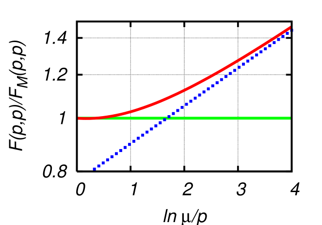
Figure 2: The resummed statistical function (46) for equal momenta $p^{\prime}=p\leq\mu$, normalized by the free-field expression (17), on a logarithmic scale. It interpolates between the free-field behavior for $p\lesssim\mu$ and the asymptotic behavior (48) (dotted line) for deep infrared momenta $p\ll\mu$. The employed parameters are $d=3$ and $\varepsilon=\sigma_{\rho}=0.1$.

The previous exact expressions take a simpler form already for moderate $|x|\gtrsim 1$ and neglecting ${\cal O}(\varepsilon)$ relative corrections in numerical coefficients. In particular, we assume that $\varepsilon\tilde{\nu}\ll\nu^{2}$, which is always true in the range of applicability of the present calculation, as discussed below. For $|x|\gtrsim 1$, we can write $\tilde{\nu}\,{\cal P}_{\alpha}(x)\pm{\rm sign}(x)\,{{\cal P}^{\prime}_{\alpha}(x)}\approx\left(\tilde{\nu}\pm{\alpha}\right){\cal P}_{\alpha}(x),$ and thus

$$\rho(x)=\Big{\{}c_{+}{\cal P}_{\bar{\nu}_{+}}(x)+c_{-}{\cal P}_{\bar{\nu}_{-}}(x)\Big{\}}e^{-\varepsilon|x|},$$ (43)

with $c_{\pm}={(\tilde{\nu}\pm\nu)/2\tilde{\nu}}$. Similarly, we have ($x\leq 0$)

$$f_{R}(x) = \left(c_{+}e^{-\bar{\nu}_{+}x}+c_{-}e^{-\bar{\nu}_{-}x}\right)e^{\varepsilon x},$$ (44)

$$f_{\sigma}(x) = -\frac{1}{4\varepsilon\tilde{\nu}}\left(e^{-\bar{\nu}_{+}x}-e^{-\bar{\nu}_{-}x}\right)e^{\varepsilon x},$$ (45)

from which we deduce, using $c_{+}c_{-}=\sigma_{\rho}/16\varepsilon^{2}\tilde{\nu}^{2}$,

$${\hat{F}^{\rm IR}(p,p^{\prime})}\!=\!\!{\sqrt{pp^{\prime}}\tilde{F}_{\nu}}\left\{c_{+}e^{-\bar{\nu}_{+}(x+x^{\prime})}+c_{-}e^{-\bar{\nu}_{-}(x+x^{\prime})}\right\}e^{\varepsilon(x+x^{\prime})},$$ (46)

with $x=\ln p/\mu$ and $x^{\prime}=\ln p^{\prime}/\mu$. Eqs. (43) and (46) are the central result of the present work. The resummation of nonlocal self-energy insertions produces a rich structure of the resummed propagator, as compared to the unperturbed one, Eqs. (17) and(18). Remarkably, it exhibits a superposition of unperturbed-like solutions with exponents $\bar{\nu}_{\pm}$, corrected by an $e^{-\varepsilon|x|}$ term which matters at large $|x|$. We see that both the spectral and statistical components of the propagator interpolate between an unperturbed (massive) behavior with exponent $\nu$ at moderate values of $|x|$ and an effective, unperturbed-like behavior with exponent $\bar{\nu}=\bar{\nu}_{+}-\varepsilon$ for very large $|x|$. This is illustrated in Fig. 2.

5 Discussion

To discuss the deep infrared behavior of the two-point correlators (43) and (46), we consider the general local quadratic action

$${\cal S}_{\rm quad}=\frac{1}{2Z}\int_{x}\varphi_{a}\left(\square-\bar{M}^{2}\right)\varphi_{a},$$ (47)

where $\bar{M}$ is an effective mass and $Z$ a field-strength renormalization factor. The corresponding correlators in a general de Sitter invariant state are easily obtained as, in the infrared limit,

$$\hat{F}_{\rm quad}^{\mathrm{IR}}(p,p^{\prime}) = \sqrt{pp^{\prime}}\,Z\,{\cal A}\,\tilde{F}_{\bar{\nu}}\,e^{-\bar{\nu}(x+x^{\prime})},$$ (48)

$$\hat{\rho}_{\rm quad}^{\mathrm{IR}}(p,p^{\prime}) = -\sqrt{pp^{\prime}}\,Z\,\mathcal{P}_{\bar{\nu}}(x-x^{\prime}),$$ (49)

with

$$\bar{\nu}=\sqrt{{d^{2}\over 4}-{\bar{M}^{2}}}$$ (50)

and where ${\cal A}$ quantifies the deviation from the Bunch-Davies vacuum (for which ${\cal A}=1$). It can be seen as a wavefunction renormalization. For the class of de Sitter invariant states, the so-called $\alpha$-vacua, ${\cal A}=|\cosh\alpha+e^{i\beta}\sinh\alpha|^{2}$ where $\alpha,\beta\in\mathbb{R}$. A deviation from unity can be seen as the result of particle production due to the field self-interactions, on top of that due to expansion.

It is easy to check that, in the deep infrared regime $|x|\gg 1$, the expressions (43) and (46) are of the form (48) and (49) with, up to relative corrections of order $\varepsilon$,

$${Z}=\frac{\tilde{\nu}+\nu}{2\tilde{\nu}}\,,\quad{\cal A}=1\quad{\rm and}\quad\frac{\bar{M}^{2}}{M^{2}}=2-\frac{\tilde{\nu}}{\nu}.$$ (51)

Note that $Z\leq 1$ and $\bar{M}^{2}/M^{2}\leq 1$. Thus we find that the general solution of the previous section is well described, in the deep infrared, by the action (47), which can thus be seen as the quadratic part of the effective action for deep infrared modes, and that there is no infrared renormalization of the vacuum state.

The effective mass $\bar{M}$ describes the power law behavior of two-point correlators in the deep infrared or, equivalently their power law decay in space-time for asymptotically large separations. This differs from the so-called dynamical mass considered in previous works [4, 35, 25], which is defined as a measure of the field fluctuations at equal points: $m_{\rm dyn}^{2}\propto 1/\langle\varphi^{2}(x)\rangle$. In particular, the latter receives contributions not only from the deep infrared regime (48), but from all infrared modes and must be evaluated from the complete expression (46). We get

$$\frac{1}{N}\langle\varphi^{2}(x)\rangle =F(x,x)=\int\frac{d^{d}p}{(2\pi)^{d}}\frac{\hat{F}(p,p)}{p}$$

$$=\frac{\Gamma(d/2)}{2\pi^{{d/2}+1}}\mu^{2\varepsilon}\left(\frac{c_{+}}{d-2(\bar{\nu}_{+}\!-\!\varepsilon)}+\frac{c_{-}}{d-2(\bar{\nu}_{-}\!-\!\varepsilon)}\right)$$

$$\equiv\frac{d\Gamma(d/2)}{4\pi^{{d/2}+1}m_{\rm dyn}^{2}},$$ (52)

where the second line corresponds to the contribution from infrared modes and the third line defines $m_{\rm dyn}$. Using Eq. (39) one easily checks that both terms in the second line contribute an infrared enhancement factor $1/\varepsilon$. We find, up to relative corrections of order $\varepsilon$,

$$\frac{m_{\rm dyn}^{2}}{M^{2}}=\frac{4}{3}\left(1-\frac{\tilde{\nu}^{2}}{4\nu^{2}}\right)\leq 1.$$ (53)

This clearly differs from the infrared mass $\bar{M}$, Eq. (51). Instead we have $m_{\rm dyn}^{2}/\bar{M}^{2}=(2+\tilde{\nu}/\nu)/3\geq 1$. This shows that the dynamical mass $m_{\rm dyn}$ employed in the literature does not characterize the asymptotic power law behavior of two-point correlators in the infrared.

We note that for coupling strong enough that $\tilde{\nu}/\nu\geq 2$, one gets an unphysical solution with both $\bar{M}^{2}\leq 0$ and $m_{\rm dyn}^{2}\leq 0$. For instance, $F(x,x)\propto\int_{\bf p}\hat{F}(p,p)/p$ is infrared finite iff $\bar{\nu}<d/2\Leftrightarrow\bar{M}^{2}>0$. Similarly, the positivity of $\langle\varphi^{2}(x)\rangle$ implies that of $m_{\rm dyn}^{2}$. Using Eqs. (38) and (51), this implies $\sigma_{\rho}<3\varepsilon^{2}(d^{2}-\varepsilon^{2})$.

Figure 3: The self-consistent local self-energy $\sigma$. The line denotes the propagator $G_{M}$, see Eq. (7).

To discuss the above results further, we now specify the mass parameter (6) which characterizes the propagator $\hat{G}_{M}$ entering the two-loop self-energy (16). As mentioned previously, for $m_{\rm dS}^{2}\leq 0$ perturbation theory is ill-defined and one has to resum a mass. The simplest scheme to do so is to include the tadpole diagram of Fig. 3 where the internal line corresponds to the propagator $G_{M}$. This is known as the Hartree approximation. In terms of the bare propagator (4), it resums the infinite series of tadpole insertions—the so-called daisy and superdaisy diagrams—and leads to a self-consistent mass. In the small mass limit one has [34, 25, 29]

$$M^{2}=m^{2}_{\mathrm{dS}}+\frac{\lambda(N+2)}{6N}\int_{\bf q}\frac{\hat{F}_{M}(q,q)}{q}\approx m^{2}_{\mathrm{dS}}+\frac{c_{d}\lambda}{M^{2}},$$ (54)

where

$$c_{d}=\frac{N+2}{12N}\frac{d\,\Gamma(d/2)}{2\pi^{d/2+1}},$$ (55)

in terms of which the parameter which controls the nonlocal self-energy corrections, see Eq. (38), reads

$$\frac{\sigma_{\rho}}{4\varepsilon^{2}\nu^{2}}=\frac{6}{N+2}\Bigg{(}\frac{c_{d}\lambda}{M^{4}}\Bigg{)}^{2}.$$ (56)

There are two interesting limits to be considered. For a massive field with $c_{d}\lambda\ll m_{\rm dS}^{4}\ll 1$, perturbation theory is well defined. Introducing $\,\bar{\!\lambda}=c_{d}\lambda/m^{4}_{\rm dS}$, we get, at the order of interest,

$${Z} = 1-\frac{3\,\bar{\!\lambda}^{2}}{2(N+2)}\,\,,$$ (57)

$$\bar{M}^{2} = m_{\rm dS}^{2}\left(1+\,\bar{\!\lambda}-\frac{N+5}{N+2}\,\bar{\!\lambda}^{2}\right)\,,$$ (58)

$$m_{\rm dyn}^{2} = m_{\rm dS}^{2}\left(1+\,\bar{\!\lambda}-\frac{N+4}{N+2}\,\bar{\!\lambda}^{2}\right).$$ (59)

The result for $m_{\rm dyn}^{2}$ agree with those from either the stochastic or Euclidean approaches in the perturbative regime for $N=1$, as recently shown in [26]. This is a highly nontrivial test of our results since, as emphasized previously, the complete solution (46) is needed to compute $m_{\rm dyn}$. We conclude that our findings equations (43)-(46) encompass the results of these approaches in the case where perturbation theory is applicable.

The other interesting limit is that of massless or light fields, with $m_{\rm dS}^{4}\ll c_{d}\lambda$. In that case, one has $M^{4}\approx c_{d}\lambda$, that is $\sigma_{\rho}/4\varepsilon^{2}\nu^{2}\sim 1$ and we get

$$\frac{\tilde{\nu}}{\nu}=\sqrt{\frac{N+8}{N+2}}.$$ (60)

It follows that $Z$, $\bar{M}^{2}/M^{2}$ and $m_{\rm dyn}^{2}/M^{2}$ are all nonperturbative in $\lambda$. These quantities actually measure the corrections to the local Hartree approximation from nonlocal self-energy insertions. The above result shows that the two-loop approximation for the latter is of the same order in coupling as the leading order (Hartree) result. This highlights the fact that the present perturbative evaluation of the self-energy (16) is not valid in that case. One should instead employ a nonperturbative approximation scheme, such as the $1/N$-expansion [40] or self-consistent 2PI techniques [25].

Finally, we mention that the case of negative tree-level mass square $m_{\rm dS}^{2}<0$, where $M^{2}=c_{d}\lambda/|m_{\rm dS}^{2}|$ [29], leads to an unphysical solution with $\bar{M}^{2}<0$. The two-loop approximation for the self-energy is certainly not valid in that case where the effective coupling $\sigma_{\rho}/2\varepsilon^{2}\nu^{2}\sim 1/\lambda^{2}$ is nonperturbatively large.

6 Conclusion

We have obtained, for the first time, an analytical solution of the Schwinger-Dyson equations for the two-point correlators at superhorizon momenta in de Sitter space, in the case of the simplest (nonlocal) two-loop self-energy. This resums the infinite series of perturbative infrared/secular logarithms and results in a rich structure as compared to the noninteracting case, with modified infrared power laws. Our results encompass those of the stochastic and Euclidean approaches in the regime of validity of perturbation theory and reveals the detailed structure of the two-point statistical and spectral correlators from horizon to deep superhorizon momenta. It is remarkable that the asymptotic infrared behavior is that of a free massive field with renormalized mass and field strength. Although it has often been assumed to be the case in the literature, this had never been firmly established. In particular, the infrared field-strength renormalization has not been considered in previous studies.

Our findings give new insight about the infrared structure of light scalar field correlators in de Sitter space. They provide useful guides for further investigations, e.g., using self-consistent resummation techniques [40]. More generally, we believe the techniques developed here and in [30] are useful tools for discussing infrared effects in the expanding de Sitter space. It is of interest to study the generalization of these tools to quasi de Sitter space relevant for inflationary cosmology. Finally, it would be interesting to extend the present techniques to the global de Sitter space and to study the resummation of the infrared divergences found in [14, 15] and argued to signal the possible quantum instability of de Sitter space.

Appendix A The two-loop self-energy

We write the two-loop self-energy of Fig. 1 as $\bar{\Sigma}=g\Pi G_{M}$, with $g=\lambda(N+2)/3N^{2}$ and where we introduced the one-loop function $\Pi=-\lambda G_{M}^{2}/6$. In the $p$-representation one has [28]

$$\hat{\Sigma}(p,p^{\prime})=g\left(pp^{\prime}\right)^{\frac{d-3}{2}}\!\!\int_{\bf q}\,\frac{r}{q}\,\hat{G}_{M}(qp,qp^{\prime})\hat{\Pi}(rp,rp^{\prime})$$ (61)

and

$$\hat{\Pi}(p,p^{\prime})=-\frac{\lambda}{6}\left(pp^{\prime}\right)^{\frac{d-3}{2}}\!\!\int_{\bf q}\,\frac{\hat{G}_{M}(qp,qp^{\prime})\hat{G}_{M}(rp,rp^{\prime})}{qr},$$ (62)

where $r=|{\bf q}+{\bf e}|$, with ${\bf e}$ a unit vector. The integral (62) has been studied in detail in Ref. [30]. In particular it has been shown there that the infrared behavior $p,p^{\prime}\lesssim\mu$ is dominated by modes $qp,qp^{\prime}\lesssim\mu$ under the integral. This condition obviously implies $rp,rp^{\prime}\lesssim\mu$ and the integrand can thus be evaluated using the low momentum behavior of the propagator $G_{M}$, see Eqs. (17) and (18). The leading infrared behavior reads

$$\hat{\Pi}_{F}^{\mathrm{IR}}(p,p^{\prime}) = -\frac{\pi_{\rho}F_{\nu}}{(pp^{\prime})^{\kappa+1/2}}\,\,,$$ (63)

$$\hat{\Pi}_{\rho}^{\mathrm{IR}}(p,p^{\prime}) = \frac{\pi_{\rho}}{\sqrt{pp^{\prime}}}\,\mathcal{P}_{\nu}^{\varepsilon}\left(\ln\frac{p}{p^{\prime}}\right),$$ (64)

where $\pi_{\rho}=\lambda F_{\nu}\Omega_{d}/6\varepsilon(2\pi)^{d}$ with $\Omega_{d}=2\pi^{d/2}/\Gamma(d/2)$, $\kappa=\nu-\varepsilon$, $F_{\nu}=\mu^{2\nu}\tilde{F}_{\nu}$ and $\mathcal{P}_{\nu}^{\varepsilon}(x)=\mathcal{P}_{\nu}(x)e^{-\varepsilon|x|}$.

A similar line of reasoning can be applied to the integral (61). The dominant infrared behavior can be obtained by restricting the integral to the region $q\lesssim\min(\mu/p,\mu/p^{\prime})$ and using the low momentum expressions (17), (18) and (63) (64) for the integrand. The evaluation of the statistical component $\hat{\Sigma}_{F}$ involves the combination $\hat{F}_{M}^{\rm IR}\hat{\Pi}_{F}^{\rm IR}-\hat{\rho}_{M}^{\rm IR}\hat{\Pi}_{\rho}^{\rm IR}/4\approx\hat{F}_{M}^{\rm IR}\hat{\Pi}_{F}^{\rm IR}$ and one gets

$$\hat{\Sigma}_{F}^{IR}(p,p^{\prime})=-\frac{gF^{2}_{\nu}\pi_{\rho}}{\left(pp^{\prime}\right)^{\,\beta+{3/2}}}\int_{\bf q}\,\,\frac{1}{q^{2\nu}r^{2\kappa}},$$ (65)

where $\beta=\nu-2\varepsilon$. The integral is rapidly convergent at high momentum and one can safely send the upper bound to infinity. The resulting integral can be evaluated by introducing Feynman parameters along the lines of [30]. We get

$$\int_{\bf q}\frac{1}{q^{2\nu}r^{2\kappa}}\!=\!\frac{\Omega_{d}}{2(2\pi)^{d}}\frac{\Gamma(\varepsilon)\Gamma(2\varepsilon)}{\Gamma(3\varepsilon)}\frac{\Gamma(\nu+\varepsilon)\Gamma(\beta)}{\Gamma(\nu)\Gamma(\beta+\varepsilon)}\!\approx\!\frac{3}{4\varepsilon}\frac{\Omega_{d}}{(2\pi)^{d}}\,\,,$$ (66)

where we neglected relative corrections of order $\varepsilon$. The final expression thus reads

$$\hat{\Sigma}_{F}^{IR}(p,p^{\prime})=-\frac{\sigma_{\rho}F_{\nu}}{(pp^{\prime})^{\,\beta+3/2}}\,\,,$$ (67)

with $\sigma_{\rho}$ given in Eq. (21). This rewrites as Eq. (19).

The spectral component $\hat{\Sigma}_{\rho}$ involves the combination $\hat{F}_{M}\hat{\Pi}_{\rho}+\hat{\rho}_{M}\hat{\Pi}_{F}$. It reads, in the case $p<p^{\prime}$,

$$\hat{\Sigma}_{\rho}^{IR}(p,p^{\prime})=g\pi_{\rho}F_{\nu}(pp^{\prime})^{\frac{d-3}{2}}\mathcal{P}_{\nu}\left(\ln\frac{p}{p^{\prime}}\right)$$

$$\times\int_{|{\bf q}|<{\mu\over p^{\prime}}}\left\{\frac{1}{(pp^{\prime})^{\kappa}}\frac{1}{r^{2\kappa}}+\frac{1}{(pp^{\prime})^{\nu}}\left({p\over p^{\prime}}\right)^{\varepsilon}\frac{1}{q^{2\nu}}\right\}.$$ (68)

The remaining integrals are easily performed (one can replace $r$ by $q$ in the denominator of the first term under the integral up to a correction of relative order $p^{\prime 2}/\mu^{2}$). After some simple algebra and repeating the calculation for the case $p>p^{\prime}$, we finally get

$$\hat{\Sigma}_{\rho}^{IR}(p,p^{\prime})=\frac{\sigma_{\rho}}{(pp^{\prime})^{{3/2}}}\mathcal{P}_{\nu}^{2\varepsilon}\left(\ln\frac{p}{p^{\prime}}\right),$$ (69)

which is Eq. (20).

References

- [1] R. Brout, S. Massar, R. Parentani and P. .Spindel, Phys. Rept. 260 (1995) 329.
- [2] D. Baumann, arXiv:0907.5424 [hep-th].
- [3] J. Bros, U. Moschella and J. P. Gazeau, Phys. Rev. Lett. 73 (1994) 1746.
- [4] A. A. Starobinsky, J. Yokoyama, Phys. Rev. D 50 (1994) 6357.
- [5] T. Prokopec, O. Tornkvist and R. P. Woodard, Phys. Rev. Lett. 89 (2002) 101301.
- [6] V. K. Onemli and R. P. Woodard, Class. Quant. Grav. 19 (2002) 4607; Phys. Rev. D 70 (2004) 107301.
- [7] T. Brunier, V. K. Onemli and R. P. Woodard, Class. Quant. Grav. 22 (2005) 59.
- [8] D. Boyanovsky, H. J. de Vega and N. G. Sanchez, Phys. Rev. D 72 (2005) 103006; Nucl. Phys. B 747 (2006) 25; M. S. Sloth, Nucl. Phys. B 748 (2006) 149-169; Nucl. Phys. B 775 (2007) 78-94; D. Seery, JCAP 0711 (2007) 025; JCAP 0802 (2008) 006.
- [9] M. van der Meulen and J. Smit, JCAP 0711 (2007) 023.
- [10] D. Marolf and I. A. Morrison, Phys. Rev. D 84 (2011) 044040; S. Hollands, Commun. Math. Phys. 319 (2013) 1-68.
- [11] A. Higuchi, D. Marolf and I. A. Morrison, Phys. Rev. D 83 (2011) 084029.
- [12] N. C. Tsamis and R. P. Woodard, Nucl. Phys. B 724 (2005) 295.
- [13] S. Weinberg, Phys. Rev. D 72 (2005) 043514; Phys. Rev. D 74 (2006) 023508.
- [14] A. M. Polyakov, Nucl. Phys. B 834 (2010) 316; arXiv:1209.4135 [hep-th].
- [15] D. Krotov and A. M. Polyakov, Nucl. Phys. B 849 (2011) 410.
- [16] B. Delamotte, Lect. Notes Phys. 852 (2012) 49-132.
- [17] J. -P. Blaizot, E. Iancu and A. Rebhan, In Quark Gluon Plama, edited by R.C. Hwa et al., (World Scientific Singapore, 2003) pp. 60-122.
- [18] J. Berges and J. Serreau, hep-ph/0302210; hep-ph/0410330; J. Berges, AIP Conf. Proc. 739 (2005) 3.
- [19] G. Lazzari and T. Prokopec, arXiv:1304.0404 [hep-th].
- [20] C. P. Burgess, L. Leblond, R. Holman and S. Shandera, JCAP 1003 (2010) 033; JCAP 1010 (2010) 017.
- [21] A. Kaya, arXiv:1303.5459 [hep-th].
- [22] S. A. Ramsey and B. L. Hu, Phys. Rev. D 56 (1997) 661.
- [23] A. Riotto and M. S. Sloth, JCAP 0804 (2008) 030.
- [24] A. Tranberg, JHEP 0811 (2008) 037.
- [25] B. Garbrecht and G. Rigopoulos, Phys. Rev. D 84 (2011) 063516.
- [26] B. Garbrecht, G. Rigopoulos and Y. Zhu, arXiv:1310.0367 [hep-th].
- [27] T. Prokopec, JCAP 1212 (2012) 023; T. Arai, Class. Quant. Grav. 29 (2012) 215014; Phys. Rev. D 86 (2012) 104064; arXiv:1304.5631 [hep-th].
- [28] R. Parentani and J. Serreau, Phys. Rev. D 87 (2013) 045020.
- [29] J. Serreau, Phys. Rev. Lett. 107 (2011) 191103.
- [30] J. Serreau and R. Parentani, Phys. Rev. D 87 (2013) 085012.
- [31] A. Youssef and D. Kreimer, arXiv:1301.3205 [gr-qc].
- [32] D. Boyanovsky and R. Holman, JHEP 1105 (2011) 047.
- [33] D. Boyanovsky, Phys. Rev. D 85 (2012) 123525; Phys. Rev. D 86 (2012) 023509.
- [34] B. L. Hu and D. J. O’Connor, Phys. Rev. Lett. 56 (1986) 1613.
- [35] A. Rajaraman, Phys. Rev. D 82 (2010) 123522; M. Beneke and P. Moch, arXiv:1212.3058 [hep-th].
- [36] D. P. Jatkar, L. Leblond and A. Rajaraman, Phys. Rev. D 85 (2012) 024047.
- [37] E. T. Akhmedov, JHEP 1201 (2012) 066; E. T. Akhmedov and P. .Burda, Phys. Rev. D 86 (2012) 044031; E. T. Akhmedov, F. K. Popov and V. M. Slepukhin, arXiv:1303.1068 [hep-th].
- [38] X. Busch and R. Parentani, Phys. Rev. D 86 (2012) 104033; J. Adamek, X. Busch and R. Parentani, Phys. Rev. D 87 (2013) 124039.
- [39] F. Gautier and J. Serreau, Phys. Rev. D 86 (2012) 125002.
- [40] F. Gautier and J. Serreau, work in progress.