Creation of quasiparticles in graphene by a time-dependent electric field

Abstract

We investigate the creation of massless quasiparticle pairs from the vacuum state in graphene by the space homogeneous time-dependent electric field. For this purpose the formalism of (2+1)-dimensional quantum electrodynamics is applied to the case of a nonstationary background with arbitrary time dependence allowing the $S$-matrix formulation of the problem. The number of created pairs per unit graphene area is expressed via the asymptotic solution at $t\to\infty$ of the second-order differential equation of an oscillator type with complex frequency satisfying some initial conditions at $t\to-\infty$. The obtained results are applied to the electric field with specific dependence on time admitting the exact solution of Dirac equation. The number of created pairs per unit area is calculated analytically in a wide variety of different regimes depending on the parameters of electric field. The investigated earlier case of static electric field is reproduced as a particular case of our formalism. It is shown that the creation rate in a time-dependent field is often larger than in a static field.

I Introduction

The creation of pairs of particles and antiparticles from the vacuum state of a quantized field by an external electromagnetic field is a familiar effect of quantum electrodynamics. It was first investigated by Schwinger 1 for the case of electron-positron pair creation by the space homogeneous static electric field. These results were later generalized for particles of arbitrary spin 2 ; 3 . Much attention was also given to the investigation of pair creation by a time-dependent space homogeneous electric field. Strictly speaking such a field can be realized in the space with a homogeneous distribution of currents. However, the approximation of a space homogeneous time-dependent electric field is also applicable in free space when the spatial size of field homogeneity is larger than the characteristic length at which a pair is created. Actually this is true in the vicinities of extremum points of the waves of E-type in waveguides 3 or of the standing waves formed by the interference of two colliding laser beams 4 . The general formalism describing the effect of pair creation by a time-dependent electric field was developed in Refs. 5 ; 6 ; 7 ; 8 and applied to fields periodic in time in Refs. 9 ; 10 . In parallel with electric field, the same effect in an external gravitational field was considered. A set of results obtained can be found in the monographs 11 for the case of electromagnetic field, 12 for the case of gravitational field and 13 for both.

Only the charged particles can be created from vacuum by the electromagnetic field. Unfortunately, even for the lightest of them, electrons, the creation rate by a static electric field $E$ becomes exponentially small for field strengths below the huge (so-called critical) value $E_{\rm cr}=m^{2}c^{3}/(|e|\hbar)\sim 10^{16}\,$V/cm, where $m$ is the electron mass and $e$ is the electron charge defined with its own (negative) sign. The same holds for a time-dependent electric field if its frequency is less then $\gamma$-frequencies (recall that the magnetic field does not create particles) 11 ; 13 . This rendered impossible the detection of particle creation by the electric field in the past. Nevertheless, the effect of particle creation was receiving widespread attention in the literature. Specifically, the back reaction of created pairs on an external electric field was studied 14 ; 15 ; 16 . The creation of pairs in strong electric field confined between two condenser plates was considered 17 (i.e., in the configuration where the Casimir effect also arises 18 ; 19 ). Recently the concept of pair creation rate was discussed 20 and the interpretation given in Ref. 21 was confirmed.

According to the recent proposal 22 , it is experimentally feasible to observe the creation of quasiparticles in graphene by the space homogeneous static electric field. Graphene is a unique material which is a one-atom-thick honeycomb lattice of carbon atoms. As a two-dimensional crystal, it possesses unusual mechanical and electrical properties 23 ; 24 . For our purposes it is most important that there are the so-called Dirac points in the energy bands of graphene. Close to Dirac points, charged quasiparticle excitations in the potential of graphene lattice are massless Dirac-like fermions characterized by a linear dispersion relation, where the Fermi velocity $v_{F}\approx 10^{-2}c$ stands in place of $c$. This holds up to the energy of about 1 eV and allows to consider graphene as the condensed matter analog for relativistic quantum field theory 22 . From this point of view the quantum ground state of a filled Fermi sea in graphene can be considered as the precise analog of a filled Dirac sea, i.e., the vacuum state for a (2+1)-dimensional field theory of massless fermions 22 . The existence of charged Fermi quasiparticles in graphene opens up outstanding possibilities to observe the effect of pair creation from vacuum in electric fields much weaker than $E_{\rm cr}$. The creation rate for quasiparticles in graphene by the space homogeneous static electric field was found in Ref. 22 using the methods of planar quantum electrodynamics in (2+1)-dimensions developed in Refs. 25 ; 26 ; 27 ; 28 ; 29 (note that in Ref. 29 the result of Ref. 22 for the creation rate of graphene quasiparticles was reobtained and confirmed). It should be emphasized also that investigations of graphene interacting with strong magnetic field 30 and with the field of an electrostatic potential barrier 31 have already led to new important physics. This makes prospective further investigation of the interaction of graphene described by the Dirac model with various electromagnetic fields.

In this paper we investigate the creation of graphene quasiparticles from vacuum by the space homogeneous time-dependent electric field. For this purpose we generalize the formalism of (2+1)-dimensional electrodynamics for the case when the electric field possesses an arbitrary time dependence [this can be done in close analogy to the (3+1)-dimensional case considered, e.g., in Refs. 7 ; 13 ]. We show that the density of created quasiparticles and holes can be expressed via solutions of the second-order differential equation of an oscillator type with complex frequency, satisfying some initial conditions, in the asymptotic region $t\to\infty$. In doing so the dependence of the electric field on time is not specified. It is only assumed that the electric field is switched off at $t\to\pm\infty$, so that the $S$-matrix formulation of the problem is possible. We further apply the obtained results to the electric field with some specific time dependence allowing an exact solution of the Dirac equation. Then we calculate the spectral density of created quasiparticles in the momentum space and respective number of pairs per unit area of graphene sheet. The analytic results are compared with the results of numerical computations for different field strengths and lifetimes. In all cases only those values of parameters are considered which fall inside the application region of the Dirac model of graphene. In the case of static electric field, the previously known results are reproduced and compared with our results obtained for a time-dependent field.

The paper is organized as follows. In Sec. II we briefly present the massless Dirac-like equation for a two-component wave function in (2+1)-dimensional space-time and construct the complete orthornormal set of solutions in the presence of a space homogeneous electric field with arbitrary time dependence. Section III contains the quantization procedure, the derivation of the Hamiltonian, allowing for interaction with a time-dependent electric field, and its diagonalization. In this section we also derive general expressions for the spectral density of created graphene quasiparticles in the momentum space and for the number of pairs created per unit area of graphene sheet. In Sec. IV we apply the obtained results to the electric field with some specific time dependence permitting an exact solution of the (2+1)-dimensional Dirac equation. Here, we calculate the spectral density and the number of graphene quasiparticles created throughout the whole lifetime of the field for different relationships among the parameters. In Sec. V we rederive the respective results for a static field in the framework of our formalism and compare the cases of time-dependent and static fields. In Sec. VI the reader will find our conclusions and discussion.

Taking into acount that our problem contains two fundamental velocities, the speed of light $c$ and the Fermi velocity in graphene $v_{F}$, and to avoid confusion, we preserve $c$, $v_{F}$ and also the Planck constant $\hbar$ in all mathematical expressions.

II Graphene in a time-dependent electric field

As was mentioned in Sec. I, the low-energy excitations in graphene are massless Dirac particles. In fact there are $N=4$ species (or flavors) of quasiparticles in graphene 22 ; 29 which can be described in a similar way. Below we consider one of them keeping in mind that the obtained number of created pairs should be multiplied by $N$. The massless particles of spin 1/2 can be described by only one two-component spinor $\xi$ which is a column with the components $\xi_{1}$, $\xi_{2}$ 32 . The respective Dirac equation for graphene is obtained by considering (2+1)-dimensional space-time and replacing $c$ with $v_{F}$ 24

$$\frac{\partial\xi}{\partial t}+v_{F}\sigma_{k}\frac{\partial\xi}{\partial x^{k}}=0,$$ (1)

where $\xi=\xi(t,\mbox{\boldmath$r$})$, $\mbox{\boldmath$r$}=(x^{1},x^{2})$, $k=1,\,2$ and $\sigma_{k}$ are the Pauli matrices

$$\sigma_{1}=\left({0{\ \ }1}\atop{1{\ \ }0}\right),\qquad\sigma_{1}=\left({0{\ }-i}\atop{i{\ \ \ \ }0}\right)$$ (2)

satisfying the standard anticommutation relations:

$$\sigma_{i}\sigma_{k}+\sigma_{k}\sigma_{i}=2\delta_{ik}.$$ (3)

In Eq. (1) and below we mean that the unit matrix stands where necessary.

We consider graphene in the space homogeneous time-dependent electric field described by the vector potential

$$A^{\mu}=\left(\Phi,\mbox{\boldmath$A$}(t)\right)=\left(0,0,A^{2}(t)\right),$$ (4)

where $\mu=0,\,1,\,2$. This field is in the plane of graphene sheet and is directed along the $x^{2}$-axis:

$$\mbox{\boldmath$E$}(t)=\left(0,0,E^{2}(t)\right),\quad E^{2}(t)=-\frac{1}{c}\,\frac{\partial A^{2}(t)}{\partial t}\equiv\frac{1}{c}A_{2}^{\prime}(t).$$ (5)

The interaction with electromagnetic field is included in Eq. (1) in the regular way by the replacement

$$i\hbar\partial_{\mu}\to i\hbar\partial_{\mu}-\frac{e}{c}A_{\mu},$$ (6)

where $\partial_{\mu}\equiv\partial/\partial{x^{\mu}}$. This leads to the following equation:

$$\left[\frac{i\hbar}{v_{F}}\frac{\partial}{\partial t}+i\hbar\sigma_{k}\frac{\partial}{\partial x^{k}}-\frac{e}{c}\sigma_{2}A_{2}(t)\right]\xi=0.$$ (7)

We seek a solution of Eq. (7) in the form

$$\xi=\left[\frac{i\hbar}{v_{F}}\frac{\partial}{\partial t}-i\hbar\sigma_{k}\frac{\partial}{\partial x^{k}}+\frac{e}{c}\sigma_{2}A_{2}(t)\right]\chi.$$ (8)

Substituting Eq. (8) in Eq. (7), one obtains the differential equation of the second order for the function $\chi$:

$$\left[\frac{\hbar^{2}}{v_{F}^{2}}\,\frac{\partial^{2}}{\partial t^{2}}-\hbar^{2}\frac{\partial^{2}}{\partial x_{1}^{2}}-\hbar^{2}\frac{\partial^{2}}{\partial x_{2}^{2}}-\frac{2ie\hbar}{c}A_{2}(t)\frac{\partial}{\partial x^{2}}\right.$$

$$~{}~{}~{}~{}~{}~{}~{}\left.\vphantom{\frac{\hbar^{2}}{v_{F}^{2}}}+\frac{e^{2}}{c^{2}}A_{2}^{2}(t)-\frac{ie\hbar}{cv_{F}}A_{2}^{\prime}(t)\sigma_{2}\right]\chi=0.$$ (9)

Solutions of Eq. (9) can be found in the form

$$\chi=\chi_{\mbox{\scriptsize\boldmath$p$},\lambda}=e^{\frac{i}{\hbar}\mbox{\scriptsize\boldmath$pr$}}f_{\lambda}(\mbox{\boldmath$p$},t)R_{\lambda},$$ (10)

where $\mbox{\boldmath$p$}=(p^{1},p^{2})$ is the momentum variable and $R_{\lambda}$ are the eigenspinors of the matrix $\sigma_{2}$ defined as

$$\sigma_{2}R_{\lambda}=\lambda R_{\lambda}.$$ (11)

From Eqs. (2) and (11) one obtains

$$\lambda=\pm 1,\qquad R_{1}=\left(1\atop i\right),\qquad R_{-1}=\left(\phantom{-}1\atop-i\right).$$ (12)

From this it follows that

$$R_{\lambda}^{+}R_{\lambda}=2,\qquad R_{1}^{+}R_{-1}=R_{-1}^{+}R_{1}=0,$$ (13)

where the cross indicates the Hermitian conjugate spinor. Substituting Eq. (10) in Eq. (9), we arrive at the following second-order ordinary differential equation of an oscillator type with complex frequency for the function $f_{\lambda}$:

$$f_{\lambda}^{\prime\prime}(\mbox{\boldmath$p$},t)+\left[\frac{v_{F}^{2}}{\hbar^{2}}\kappa^{2}(\mbox{\boldmath$p$},t)-\frac{i\lambda ev_{F}}{\hbar c}A_{2}^{\prime}(t)\right]f_{\lambda}(\mbox{\boldmath$p$},t)=0,$$ (14)

where

$$\kappa^{2}(\mbox{\boldmath$p$},t)=p_{1}^{2}+\left[p_{2}-\frac{e}{c}A_{2}(t)\right]^{2}.$$ (15)

Using Eqs. (8), (10) and (11) it is easily seen that solutions of Eq. (7) satisfy the equality

$$\xi_{\mbox{\scriptsize\boldmath$p$},\lambda^{\prime}}^{+}\xi_{\mbox{\scriptsize\boldmath$p$},\lambda}=\frac{\hbar^{2}}{v_{F}^{2}}{\chi_{\mbox{\scriptsize\boldmath$p$},\lambda^{\prime}}^{+}}^{\!\!\!\!\!\prime}\,\,\,\chi_{\mbox{\scriptsize\boldmath$p$},\lambda}^{\,\prime}$$

$$~{}~{}~{}~{}~{}~{}~{}~{}~{}+\left[p_{1}^{2}+\lambda\lambda^{\prime}\left(p_{2}-\frac{e}{c}A_{2}\right)^{2}\right]\chi_{\mbox{\scriptsize\boldmath$p$},\lambda^{\prime}}^{+}\,\chi_{\mbox{\scriptsize\boldmath$p$},\lambda}$$ (16)

$$~{}~{}~{}~{}~{}~{}~{}~{}~{}+\frac{i\hbar}{v_{F}}\left(p_{2}-\frac{e}{c}A_{2}\right)\,\left(\lambda{\chi_{\mbox{\scriptsize\boldmath$p$},\lambda^{\prime}}^{+}}^{\!\!\!\!\!\prime}\,\,\,\chi_{\mbox{\scriptsize\boldmath$p$},\lambda}-\lambda^{\prime}\chi_{\mbox{\scriptsize\boldmath$p$},\lambda^{\prime}}^{+}\,\chi_{\mbox{\scriptsize\boldmath$p$},\lambda}^{\,\prime}\right).$$

For $\lambda^{\prime}\neq\lambda$ with the help of Eq. (13) this leads to

$$\xi_{\mbox{\scriptsize\boldmath$p$},\lambda^{\prime}}^{+}\xi_{\mbox{\scriptsize\boldmath$p$},\lambda}=0.$$ (17)

For $\lambda^{\prime}=\lambda$ Eqs. (13) and (16) result in

$$\xi_{\mbox{\scriptsize\boldmath$p$},\lambda}^{+}\xi_{\mbox{\scriptsize\boldmath$p$},\lambda}=2\left[\frac{\hbar^{2}}{v_{F}^{2}}\left|f_{\lambda}^{\prime}\right|^{2}+\kappa^{2}(\mbox{\boldmath$p$},t)\left|f_{\lambda}\right|^{2}\right.$$

$$~{}~{}~{}~{}~{}~{}~{}\left.-\frac{2\hbar\lambda}{v_{F}}\left(p_{2}-\frac{e}{c}A_{2}\right)\,\mbox{Im}(f_{\lambda}{f_{\lambda}^{\ast}}^{\prime})\right].$$ (18)

By the differentiation of both sides of Eq. (18), using Eq. (14), one obtains

$$\frac{d}{dt}\left(\xi_{\mbox{\scriptsize\boldmath$p$},\lambda}^{+}\xi_{\mbox{\scriptsize\boldmath$p$},\lambda}\right)=0.$$ (19)

This means that the quantity (18) does not depend on time and can be made equal to any number depending on the initial conditions imposed on functions $f_{\lambda}(\mbox{\boldmath$p$},t)$ satisfying Eq. (14).

We assume that the external field (5) is switched off at $t\to\pm\infty$, so that the vector potential (2) has finite limiting values

$$A_{2,\pm}=\lim_{t\to\pm\infty}A_{2}(t).$$ (20)

Then we impose the following initial conditions on the solutions of Eq. (14):

$$f_{\lambda}(\mbox{\boldmath$p$},t)\big{|}_{t\to-\infty}=C_{\mbox{\scriptsize\boldmath$p$}},$$

$$f_{\lambda}^{\prime}(\mbox{\boldmath$p$},t)\big{|}_{t\to-\infty}=-\frac{i\lambda v_{F}}{\hbar}\kappa_{-}(\mbox{\boldmath$p$})C_{\mbox{\scriptsize\boldmath$p$}},$$ (21)

where

$$\kappa_{\pm}(\mbox{\boldmath$p$})\equiv\lim_{t\to\pm\infty}\kappa(\mbox{\boldmath$p$},t),$$

$$C_{\mbox{\scriptsize\boldmath$p$}}=\frac{1}{2\kappa_{-}^{1/2}\left[\kappa_{-}-\left(p_{2}-\frac{e}{c}A_{2,-}\right)\right]^{1/2}}.$$ (22)

According to Eq. (21), the solutions $f_{1}(\mbox{\boldmath$p$},t)$ and $f_{-1}(\mbox{\boldmath$p$},t)$ can be called the positive- and negative-frequency solutions of Eq. (14), respectively. In a similar way, the solutions $\chi_{\mbox{\scriptsize\boldmath$p$},1}$, $\chi_{\mbox{\scriptsize\boldmath$p$},-1}$ from Eq. (10) and also $\xi_{\mbox{\scriptsize\boldmath$p$},1}$, $\xi_{\mbox{\scriptsize\boldmath$p$},-1}$, obtained from them by using Eq. (8), are also called the positive- and negative-frequency solutions, respectively. From Eqs. (14) and (21) it follows that $f_{1}^{\ast}(\mbox{\boldmath$p$},t)=f_{-1}(\mbox{\boldmath$p$},t)$.

With the chosen initial conditions (21) and (22), it is easily seen that at $t\to-\infty$ (and, thus, at any $t$) the quantity (18) is equal to unity. Thus, from Eqs. (17) and (18) one obtains at any $\lambda^{\prime}$ and $\lambda$:

$$\xi_{\mbox{\scriptsize\boldmath$p$},\lambda^{\prime}}^{+}(t,\mbox{\boldmath$r$})\xi_{\mbox{\scriptsize\boldmath$p$},\lambda}(t,\mbox{\boldmath$r$})=\delta_{\lambda\lambda^{\prime}}.$$ (23)

Specifically for $\lambda^{\prime}=\lambda$ from Eq. (18) we arrive at an important identity

$$\frac{\hbar^{2}}{v_{F}^{2}}\left|f_{\lambda}^{\prime}\right|^{2}+\kappa^{2}(\mbox{\boldmath$p$},t)\left|f_{\lambda}\right|^{2}-\frac{2\hbar\lambda}{v_{F}}\left(p_{2}-\frac{e}{c}A_{2}\right)\,\mbox{Im}(f_{\lambda}{f_{\lambda}^{\ast}}^{\prime})=\frac{1}{2},$$ (24)

which will be used in Sec. III.

Now, using Eqs. (8), (10) and (11), we obtain

$$\int\xi_{\mbox{\scriptsize\boldmath$p$}^{\prime},\lambda^{\prime}}^{+}(t,\mbox{\boldmath$r$})\xi_{\mbox{\scriptsize\boldmath$p$},\lambda}(t,\mbox{\boldmath$r$})d^{2}r=(2\pi)^{2}\delta^{2}\left(\frac{\mbox{\boldmath$p$}-\mbox{\boldmath$p$}^{\prime}}{\hbar}\right)\delta_{\lambda\lambda^{\prime}}.$$ (25)

As a result, the function $\xi_{\mbox{\scriptsize\boldmath$p$},\lambda}$ defined above form the complete orthornormal set of solutions of the massless (2+1)-dimensional Dirac equation (7).

III Hamiltonian, its diagonalization and the density of created quasiparticles

With the help of a complete orthornormal set of solutions of Eq. (7) found in Sec. II the operator of a quantized field of low-energy quasiparticles in graphene can be written in the form

$$\xi(t,\mbox{\boldmath$r$})=\frac{1}{2\pi\hbar}\int d^{2}p\left[\xi_{\mbox{\scriptsize\boldmath$p$},1}(t,\mbox{\boldmath$r$})a_{\mbox{\scriptsize\boldmath$p$}}+\xi_{-\mbox{\scriptsize\boldmath$p$},-1}(t,\mbox{\boldmath$r$})b_{\mbox{\scriptsize\boldmath$p$}}^{+}\right],$$

(26)

$$\xi^{+}(t,\mbox{\boldmath$r$})=\frac{1}{2\pi\hbar}\int d^{2}p^{\prime}\left[\xi_{\mbox{\scriptsize\boldmath$p$}^{\prime},1}^{+}(t,\mbox{\boldmath$r$})a_{\mbox{\scriptsize\boldmath$p$}^{\prime}}^{+}+\xi_{-\mbox{\scriptsize\boldmath$p$}^{\prime},-1}^{+}(t,\mbox{\boldmath$r$})b_{\mbox{\scriptsize\boldmath$p$}^{\prime}}\right].$$

Here, $a_{\mbox{\scriptsize\boldmath$p$}},{\ }a_{\mbox{\scriptsize\boldmath$p$}}^{+}$ and $b_{\mbox{\scriptsize\boldmath$p$}},{\ }b_{\mbox{\scriptsize\boldmath$p$}}^{+}$ are the annihilation and creation operators of quasiparticles and antiquasiparticles (holes), respectively, satisfying the standard anticommutation relations

$$[a_{\mbox{\scriptsize\boldmath$p$}},a_{\mbox{\scriptsize\boldmath$p$}^{\prime}}^{+}]=[b_{\mbox{\scriptsize\boldmath$p$}},b_{\mbox{\scriptsize\boldmath$p$}^{\prime}}^{+}]=\delta^{2}(\mbox{\boldmath$p$}-\mbox{\boldmath$p$}^{\prime}).$$ (27)

Unlike the case of a massive spinor field, the field operators (26) do not contain summations in the double-valued spin indices. There is also no dependence on spin indices in the creation and annihilation operators which depend only on the momentum quantum numbers. The reason is that in a massless case the fermion states with definite momentum are characterized by the fixed helicity (or chirality), i.e., the projection of a spin (pseudospin) on the direction of momentum is fixed 32 . Thus, for quasiparticles in Eq. (26) this projection is positive ($\lambda=1$) and for antiparticles (holes) — negative ($\lambda=-1$).

The Hamiltonian of the quantized field (26) is expressed via the 00-component of the stress-energy tensor

$$H(t)=\int d^{2}rT_{00}(t,\mbox{\boldmath$r$})$$ (28)

$$~{}~{}~{}=\frac{i\hbar}{2}\int d^{2}r\left[\xi^{+}(t,\mbox{\boldmath$r$})\frac{\partial\xi(t,\mbox{\boldmath$r$})}{\partial t}-\frac{\partial\xi^{+}(t,\mbox{\boldmath$r$})}{\partial t}\xi(t,\mbox{\boldmath$r$})\right].$$

Now we substitute Eq. (26) in Eq. (28) and perform the following identical transformations. First, we integrate with respect to $r$ by using Eqs. (8), (10) and (13). Then the delta-functions of the form $\delta^{2}[(\mbox{\boldmath$p$}-\mbox{\boldmath$p$}^{\prime})/\hbar]$ and $\delta^{2}[(\mbox{\boldmath$p$}+\mbox{\boldmath$p$}^{\prime})/\hbar]$ produced from this integration are used to integrate with respect to $\mbox{\boldmath$p$}^{\prime}$. As a result, by changing the integration variable $p$ for $-\mbox{\boldmath$p$}$ where appropriate, we bring the Hamiltonian to the form

$$H(t)=\hbar\int d^{2}p\left[B_{1,1}(\mbox{\boldmath$p$},t)a_{\mbox{\scriptsize\boldmath$p$}}^{+}\,a_{\mbox{\scriptsize\boldmath$p$}}+B_{1,-1}(\mbox{\boldmath$p$},t)a_{\mbox{\scriptsize\boldmath$p$}}^{+}\,b_{-\mbox{\scriptsize\boldmath$p$}}^{+}\right.$$

$$~{}~{}~{}\left.+B_{-1,1}(\mbox{\boldmath$p$},t)b_{-\mbox{\scriptsize\boldmath$p$}}\,a_{\mbox{\scriptsize\boldmath$p$}}+B_{-1,-1}(\mbox{\boldmath$p$},t)b_{-\mbox{\scriptsize\boldmath$p$}}\,b_{-\mbox{\scriptsize\boldmath$p$}}^{+}\right],$$ (29)

where the coefficients $B_{\lambda,\lambda^{\prime}}(\mbox{\boldmath$p$},t)$ are defined as

$$B_{\lambda,\lambda^{\prime}}(\mbox{\boldmath$p$},t)=\frac{i}{2}\left(\xi_{\mbox{\scriptsize\boldmath$p$},\lambda}^{+}\,\xi_{\mbox{\scriptsize\boldmath$p$},\lambda^{\prime}}^{\prime}-{\xi_{\mbox{\scriptsize\boldmath$p$},\lambda}^{+}}^{\!\!\!\prime}\,\,\xi_{\mbox{\scriptsize\boldmath$p$},\lambda^{\prime}}\right).$$ (30)

Using Eq. (23), one can rearrange Eq. (30) to

$$B_{\lambda,\lambda^{\prime}}(\mbox{\boldmath$p$},t)=i\xi_{\mbox{\scriptsize\boldmath$p$},\lambda}^{+}\,\xi_{\mbox{\scriptsize\boldmath$p$},\lambda^{\prime}}^{\prime}$$ (31)

With the help of Eqs. (8) and (12)–(14) the coefficients (31) can be expressed in terms of the function $f_{-1}\equiv f_{-1}(\mbox{\boldmath$p$},t)$ satisfying Eq. (14) with the initial conditions (21):

$$B_{1,1}(\mbox{\boldmath$p$},t)=-B_{-1,-1}(\mbox{\boldmath$p$},t)=4\kappa^{2}(\mbox{\boldmath$p$},t)\,\mbox{Im}(f_{-1}^{\ast}f_{-1}^{\prime})$$

$$~{}~{}-2\left[p_{2}-\frac{e}{c}A_{2}(t)\right]\,\left[\frac{\hbar}{v_{F}}|f_{-1}^{\prime}|^{2}+\frac{v_{F}}{\hbar}\kappa^{2}(\mbox{\boldmath$p$},t)|f_{-1}|^{2}\right],$$ (32)

$$B_{1,-1}(\mbox{\boldmath$p$},t)=B_{-1,1}^{\ast}(\mbox{\boldmath$p$},t)=2ip_{1}\left[\frac{\hbar}{v_{F}}{f_{-1}^{\prime}}^{\!\!\!\!2}+\frac{v_{F}}{\hbar}\kappa^{2}(\mbox{\boldmath$p$},t)f_{-1}^{2}\right].$$

The use of the identity (24) allows to rearrange the coefficient $B_{1,1}(\mbox{\boldmath$p$},t)$ in Eq. (32) to a more simple form

$$B_{1,1}(\mbox{\boldmath$p$},t)=4p_{1}^{2}\,\mbox{Im}(f_{-1}^{\ast}f_{-1}^{\prime})-\frac{v_{F}}{\hbar}\,\left[p_{2}-\frac{e}{c}A_{2}(t)\right].$$ (33)

As can be seen from Eq. (29), at any $t>-\infty$, i.e., in the presence of the external electric field (5), the Hamiltonian is a nondiagonal quadratic form in terms of the creation-annihilation operators of quasiparticles. However, at $t\to-\infty$, when the electric field (5) is switched off, the initial conditions (21) lead to

$$B_{1,1}(\mbox{\boldmath$p$},t)\to 0,\qquad B_{1,-1}(\mbox{\boldmath$p$},t)\to\frac{v_{F}}{\hbar}\kappa_{-}(\mbox{\boldmath$p$}).$$ (34)

As a result, the Hamiltonian (29) takes the diagonal form

$$H(-\infty)=v_{F}\int d^{2}p\left(a_{\mbox{\scriptsize\boldmath$p$}}^{+}\,a_{\mbox{\scriptsize\boldmath$p$}}-b_{-\mbox{\scriptsize\boldmath$p$}}\,b_{-\mbox{\scriptsize\boldmath$p$}}^{+}\right),$$ (35)

as it should be for a Hamiltonian of free noninteracting particles.

The nondiagonality of the Hamiltonian at $t>-\infty$ points to the fact that the time-dependent electric field creates pairs of particles and antiparticles from the initial vacuum state $|0_{\rm in}\rangle$ defined at $t\to-\infty$ by the equations

$$a_{\mbox{\scriptsize\boldmath$p$}}|0_{\rm in}\rangle=b_{\mbox{\scriptsize\boldmath$p$}}|0_{\rm in}\rangle=0.$$ (36)

To investigate the effect of particle creation, it is convenient to introduce the notations

$$E(\mbox{\boldmath$p$},t)=\frac{B_{1,1}(\mbox{\boldmath$p$},t)}{\kappa(\mbox{\boldmath$p$},t)},\quad F(\mbox{\boldmath$p$},t)=\frac{B_{1,-1}(\mbox{\boldmath$p$},t)}{\kappa(\mbox{\boldmath$p$},t)},$$ (37)

where $B_{1,1}(\mbox{\boldmath$p$},t)$ is defined in Eq. (33) and $B_{1,-1}(\mbox{\boldmath$p$},t)$ in Eq. (32). Then, with account of Eq. (32), the Hamiltonian (29) takes the form

$$H(t)=\hbar\int d^{2}p\,\kappa(\mbox{\boldmath$p$},t)\left[E(\mbox{\boldmath$p$},t)\left(a_{\mbox{\scriptsize\boldmath$p$}}^{+}\,a_{\mbox{\scriptsize\boldmath$p$}}-b_{-\mbox{\scriptsize\boldmath$p$}}\,b_{-\mbox{\scriptsize\boldmath$p$}}^{+}\right)\right.$$

$$~{}~{}~{}~{}~{}+\left.F(\mbox{\boldmath$p$},t)\,a_{\mbox{\scriptsize\boldmath$p$}}^{+}\,b_{-\mbox{\scriptsize\boldmath$p$}}^{+}+F^{\ast}(\mbox{\boldmath$p$},t)\,b_{-\mbox{\scriptsize\boldmath$p$}}\,a_{\mbox{\scriptsize\boldmath$p$}}\right].$$ (38)

The coefficients (37) satisfy the condition

$$E^{2}(\mbox{\boldmath$p$},t)+|F(\mbox{\boldmath$p$},t)|^{2}=\frac{v_{F}^{2}}{\hbar^{2}}.$$ (39)

To see this, we substitute Eqs. (32), (33) and (37) to the left-hand side of Eq. (39) and express the quantity $\mbox{Im}(f_{-1}^{\ast}f_{-1}^{\prime})$ from the identity (24). After transformations, using an evident identity

$$\mbox{Re}\,z^{2}=|z|^{2}-2\,\mbox{Im}^{2}z$$ (40)

with $z={f_{-1}^{\ast}}^{\!\!\!\prime}\,f_{-1}$, one arrives at Eq. (39).

Now we take into account that at $t\to\infty$, when the time-dependent electric field is switched off, the Hamiltonian (38) should describe free particles and, thus, should be the diagonal quadratic form (here we neglect by the interaction between particles through the exchange of virtual photons). In fact it is even possible to diagonalize the Hamiltonian at any $t$, although in the presence of an external field the concept of “free” particle can be considered as somewhat formal. To diagonalize the Hamiltonian (38) at any $t$, we introduce the time-dependent creation and annihilation operators for particles, $c_{\mbox{\scriptsize\boldmath$p$}}^{+}(t)$, $c_{\mbox{\scriptsize\boldmath$p$}}(t)$, and respective operators for antiparticles, $d_{\mbox{\scriptsize\boldmath$p$}}^{+}(t)$, $d_{\mbox{\scriptsize\boldmath$p$}}(t)$, connected with the in-operators, $a_{\mbox{\scriptsize\boldmath$p$}}^{+}$, $a_{\mbox{\scriptsize\boldmath$p$}}$ and $b_{\mbox{\scriptsize\boldmath$p$}}^{+}$, $b_{\mbox{\scriptsize\boldmath$p$}}$, by means of the Bogoliubov transformations

$$a_{\mbox{\scriptsize\boldmath$p$}}=\alpha_{\mbox{\scriptsize\boldmath$p$}}^{\ast}(t)\,c_{\mbox{\scriptsize\boldmath$p$}}(t)-\beta_{\mbox{\scriptsize\boldmath$p$}}(t)\,d_{-\mbox{\scriptsize\boldmath$p$}}^{+}(t),$$

$$b_{\mbox{\scriptsize\boldmath$p$}}=\alpha_{-\mbox{\scriptsize\boldmath$p$}}^{\ast}(t)\,d_{\mbox{\scriptsize\boldmath$p$}}(t)+\beta_{-\mbox{\scriptsize\boldmath$p$}}(t)\,c_{-\mbox{\scriptsize\boldmath$p$}}^{+}(t).$$ (41)

The two equations Hermitian conjugate to Eq. (41) are also needed. The $c$-number coefficients of the Bogoliubov transformations, $\alpha_{\mbox{\scriptsize\boldmath$p$}}(t)$ and $\beta_{\mbox{\scriptsize\boldmath$p$}}(t)$, satisfy the condition

$$|\alpha_{\mbox{\scriptsize\boldmath$p$}}(t)|^{2}+|\beta_{\mbox{\scriptsize\boldmath$p$}}(t)|^{2}=1,$$ (42)

which assures the reversibility of these transformations. Using Eq. (42), it can be easily seen also that the time-dependent operators, $c_{\mbox{\scriptsize\boldmath$p$}}^{+}(t)$, $c_{\mbox{\scriptsize\boldmath$p$}}(t)$ and $d_{\mbox{\scriptsize\boldmath$p$}}^{+}(t)$, $d_{\mbox{\scriptsize\boldmath$p$}}(t)$, at any $t$ satisfy the same anticommutation relations (27), as the in-operators. The time-dependent vacuum state can be defined as

$$c_{\mbox{\scriptsize\boldmath$p$}}(t)|0_{t}\rangle=d_{\mbox{\scriptsize\boldmath$p$}}(t)|0_{t}\rangle=0.$$ (43)

If, as in our case, there is an external field at finite $t$ which creates pairs, $|0_{t}\rangle\neq|0_{\rm in}\rangle$, i.e., the vacuum state is unstable.

Now we are in a position to diagonalize the Hamiltonian (38). Substituting Eq. (41) and Hermitian conjugate to it in Eq. (38), one obtains

$$H(t)=\hbar\int d^{2}p\,\kappa(\mbox{\boldmath$p$},t)\left\{\left[E(\mbox{\boldmath$p$},t)\left(|\alpha_{\mbox{\scriptsize\boldmath$p$}}(t)|^{2}-|\beta_{\mbox{\scriptsize\boldmath$p$}}(t)|^{2}\right)+F(\mbox{\boldmath$p$},t)\alpha_{\mbox{\scriptsize\boldmath$p$}}(t)\beta_{\mbox{\scriptsize\boldmath$p$}}^{\ast}(t)\right.\right.$$ (44)

$$~{}~{}~{}\left.+F^{\ast}(\mbox{\boldmath$p$},t)\alpha_{\mbox{\scriptsize\boldmath$p$}}^{\ast}(t)\beta_{\mbox{\scriptsize\boldmath$p$}}(t)\right]\!\left[c_{\mbox{\scriptsize\boldmath$p$}}^{+}(t)\,c_{\mbox{\scriptsize\boldmath$p$}}(t)-d_{-\mbox{\scriptsize\boldmath$p$}}(t)\,d_{-\mbox{\scriptsize\boldmath$p$}}^{+}(t)\right]$$

$$~{}~{}~{}+\left[F(\mbox{\boldmath$p$},t)\,\alpha_{\mbox{\scriptsize\boldmath$p$}}^{2}(t)-F^{\ast}(\mbox{\boldmath$p$},t)\,\beta_{\mbox{\scriptsize\boldmath$p$}}^{2}(t)-2E(\mbox{\boldmath$p$},t)\alpha_{\mbox{\scriptsize\boldmath$p$}}(t)\,\beta_{\mbox{\scriptsize\boldmath$p$}}(t)\right]c_{\mbox{\scriptsize\boldmath$p$}}^{+}(t)\,d_{-\mbox{\scriptsize\boldmath$p$}}^{+}(t)$$

$$~{}~{}~{}\left.+\left[F^{\ast}(\mbox{\boldmath$p$},t)\,{\alpha_{\mbox{\scriptsize\boldmath$p$}}^{\ast}}^{2}(t)-F(\mbox{\boldmath$p$},t)\,{\beta_{\mbox{\scriptsize\boldmath$p$}}^{\ast}}^{2}(t)-2E(\mbox{\boldmath$p$},t)\,{\alpha_{\mbox{\scriptsize\boldmath$p$}}^{\ast}}(t)\,{\beta_{\mbox{\scriptsize\boldmath$p$}}^{\ast}}(t)\right]d_{-\mbox{\scriptsize\boldmath$p$}}(t)\,c_{\mbox{\scriptsize\boldmath$p$}}(t)\right\}.$$

To bring the quadratic in creation-annihilation operators expression in Eq. (44) to a diagonal form, we demand that

$$F(\mbox{\boldmath$p$},t)\,\alpha_{\mbox{\scriptsize\boldmath$p$}}^{2}(t)-F^{\ast}(\mbox{\boldmath$p$},t)\,\beta_{\mbox{\scriptsize\boldmath$p$}}^{2}(t)-2E(\mbox{\boldmath$p$},t)\alpha_{\mbox{\scriptsize\boldmath$p$}}(t)\,\beta_{\mbox{\scriptsize\boldmath$p$}}(t)=0,$$ (45)

which leads to the quadratic equation

$$F^{\ast}(\mbox{\boldmath$p$},t)\left[\frac{\beta_{\mbox{\scriptsize\boldmath$p$}}(t)}{\alpha_{\mbox{\scriptsize\boldmath$p$}}(t)}\right]^{2}+2E(\mbox{\boldmath$p$},t)\frac{\beta_{\mbox{\scriptsize\boldmath$p$}}(t)}{\alpha_{\mbox{\scriptsize\boldmath$p$}}(t)}-F(\mbox{\boldmath$p$},t)=0.$$ (46)

By solving this equation with account of the identity (39), one arrives at

$$\frac{\beta_{\mbox{\scriptsize\boldmath$p$}}(t)}{\alpha_{\mbox{\scriptsize\boldmath$p$}}(t)}=\frac{-E(\mbox{\boldmath$p$},t)\pm\sqrt{E^{2}(\mbox{\boldmath$p$},t)+|F(\mbox{\boldmath$p$},t)|^{2}}}{F^{\ast}(\mbox{\boldmath$p$},t)}$$

$$~{}~{}~{}~{}~{}~{}~{}~{}=\frac{-E(\mbox{\boldmath$p$},t)\pm(v_{F}/\hbar)}{F^{\ast}(\mbox{\boldmath$p$},t)}.$$ (47)

Then, using Eq. (42), one finds from Eq. (47)

$$|\beta_{\mbox{\scriptsize\boldmath$p$}}(t)|^{2}=\frac{1}{2}\left[1\mp\frac{\hbar}{v_{F}}E(\mbox{\boldmath$p$},t)\right].$$ (48)

To satisfy the condition $\beta_{\mbox{\scriptsize\boldmath$p$}}(t)=0$ at $t\to-\infty$ when there is no pair creation, the upper sign on the right-hand side of Eqs. (47) and (48) should be chosen because, in accordance with the initial conditions (21) and (22), $E(\mbox{\boldmath$p$},t)\to v_{F}/\hbar$ when $t\to-\infty$ [see Eqs. (34) and (37)]. As a result, we have

$$|\beta_{\mbox{\scriptsize\boldmath$p$}}(t)|^{2}=\frac{1}{2}\left[1-\frac{\hbar}{v_{F}}E(\mbox{\boldmath$p$},t)\right].$$ (49)

Using Eqs. (47) with the upper sign and (49), the coefficient near the diagonal terms in the Hamiltonian (44) can be easily calculated

$$E(\mbox{\boldmath$p$},t)\left(|\alpha_{\mbox{\scriptsize\boldmath$p$}}(t)|^{2}-|\beta_{\mbox{\scriptsize\boldmath$p$}}(t)|^{2}\right)+F(\mbox{\boldmath$p$},t)\alpha_{\mbox{\scriptsize\boldmath$p$}}(t)\beta_{\mbox{\scriptsize\boldmath$p$}}^{\ast}(t)$$

$$~{}~{}~{}~{}~{}~{}~{}~{}~{}~{}~{}~{}~{}~{}~{}~{}~{}~{}+F^{\ast}(\mbox{\boldmath$p$},t)\alpha_{\mbox{\scriptsize\boldmath$p$}}^{\ast}(t)\beta_{\mbox{\scriptsize\boldmath$p$}}(t)=\frac{v_{F}}{\hbar}.$$ (50)

Finally, the Hamiltonian (44) takes the form

$$H(t)=v_{F}\int d^{2}p\,\kappa(\mbox{\boldmath$p$},t)\left[c_{\mbox{\scriptsize\boldmath$p$}}^{+}(t)\,c_{\mbox{\scriptsize\boldmath$p$}}(t)-d_{-\mbox{\scriptsize\boldmath$p$}}(t)\,d_{-\mbox{\scriptsize\boldmath$p$}}^{+}(t)\right],$$ (51)

i.e., it is diagonal at any $t$ in terms of time-dependent creation-annihilation operators.

In order to describe the creation of real particles (quasiparticles), we consider the asymptotic limit $t\to\infty$ when the external field is switched off. In this limiting case the operators $c_{\mbox{\scriptsize\boldmath$p$}}$, $c_{\mbox{\scriptsize\boldmath$p$}}^{+}$ and $d_{\mbox{\scriptsize\boldmath$p$}}$, $d_{\mbox{\scriptsize\boldmath$p$}}^{+}$ are the operators of real particles and the vacuum state $|0_{\infty}\rangle=|0_{\rm out}\rangle$. Using the Bogoliubov transformations inverse to (41), we find the spectral density of quasiparticles and antiquasiparticles (holes) created in graphene during all time when the electric field was switched on

$$N_{\mbox{\scriptsize\boldmath$p$}}=\langle 0_{\rm in}|c_{\mbox{\scriptsize\boldmath$p$}}^{+}(\infty)\,c_{\mbox{\scriptsize\boldmath$p$}}(\infty)|0_{\rm in}\rangle=\langle 0_{\rm in}|d_{-\mbox{\scriptsize\boldmath$p$}}^{+}(\infty)\,d_{-\mbox{\scriptsize\boldmath$p$}}(\infty)|0_{\rm in}\rangle$$

$$~{}~{}~{}=|\beta_{\mbox{\scriptsize\boldmath$p$}}(\infty)|^{2}\delta^{2}(\mbox{\boldmath$p$}=0)=|\beta_{\mbox{\scriptsize\boldmath$p$}}(\infty)|^{2}\frac{S}{(2\pi\hbar)^{2}},$$ (52)

where $S$ is the graphene area which is supposed to be sufficiently large. Then the spectral density of created pairs per unit area of graphene is given by

$$n_{\mbox{\scriptsize\boldmath$p$}}=\frac{N_{\mbox{\scriptsize\boldmath$p$}}}{S}=\frac{1}{(2\pi\hbar)^{2}}|\beta_{\mbox{\scriptsize\boldmath$p$}}|^{2},$$ (53)

where in accordance with Eqs. (32), (37) and (49) $|\beta_{\mbox{\scriptsize\boldmath$p$}}|^{2}$ is defined as

$$|\beta_{\mbox{\scriptsize\boldmath$p$}}|^{2}\equiv|\beta_{\mbox{\scriptsize\boldmath$p$}}(\infty)|^{2}=\frac{1}{2}\left[1-\frac{\hbar}{v_{F}}E(\mbox{\boldmath$p$})\right],$$ (54)

$$E(\mbox{\boldmath$p$})=\lim_{t\to\infty}E(\mbox{\boldmath$p$},t)=\frac{4p_{1}^{2}}{\kappa_{+}}\,\mbox{Im}(f_{-1,+}^{\ast}f_{-1,+}^{\prime})-\frac{v_{F}}{\hbar\kappa_{+}}\left(p_{2}-\frac{e}{c}A_{2,+}\right),$$

$$f_{-1,+}\equiv f_{-1,+}(\mbox{\boldmath$p$})=\lim_{t\to\infty}f_{-1}(\mbox{\boldmath$p$},t).$$

The net number of pairs created with all momenta (note that the momenta of created quasiparticle and hole take the opposite values because in the space homogeneous field the momentum is conserved) is obtained by the integration of Eq. (53)

$$n=\int d^{2}p\,n_{\mbox{\scriptsize\boldmath$p$}}=\frac{1}{(2\pi\hbar)^{2}}\int d^{2}p\,|\beta_{\mbox{\scriptsize\boldmath$p$}}|^{2}.$$ (55)

Keeping in mind that there are $N=4$ species of quasiparticles in graphene, for the total number of created pairs per unit area one finally obtains

$$n_{\rm tot}=4n=\frac{1}{\pi^{2}\hbar^{2}}\int d^{2}p\,|\beta_{\mbox{\scriptsize\boldmath$p$}}|^{2}.$$ (56)

Equations (54), (49) and (56) express $n_{\rm tot}$ via the asymptotic solution of Eq. (14) with the initial conditions (21). This solution can be found, either analytically or numerically, when the time-dependent electric field (4), (5) is specified.

IV Creation of graphene quasiparticles by a single pulse of electric field

As an exactly solvable example we consider the electric field of the form

$$A^{2}(t)=-\frac{E_{0}c}{\Omega}\,\tanh(\Omega t),\qquad E^{2}(t)=\frac{E_{0}}{\cosh^{2}(\Omega t)},$$ (57)

which goes to zero at $t\to\pm\infty$. Here $E_{0}=\mbox{const}$ is the maximum strength of the field achieved at $t=0$. The effect of creation of massive spinor particles by this field was considered in Ref. 33 in (3+1)-dimensional space-time. Substituting Eq. (57) in Eq. (14) one obtains the following exact solution satisfying the initial conditions (21) (compare with Ref. 33 ):

$$f_{-1}(\mbox{\boldmath$p$},t)=C_{\mbox{\scriptsize\boldmath$p$}}\,e^{i{v_{F}\kappa_{-}(\mbox{\scriptsize\boldmath$p$})t}/{\hbar}}(1+e^{2\Omega t})^{-i{\theta}/{\pi}}{}_{2}F_{1}(\mu,\nu;\gamma;-e^{2\Omega t}),$$ (58)

where $C_{\mbox{\scriptsize\boldmath$p$}}$ is defined in Eq. (21), ${}_{2}F_{1}(\mu,\nu;\gamma;z)$ is the hypergeometric function, and all the other notations are:

$$\kappa_{\pm}^{2}=p_{1}^{2}+\left(p_{2}\mp\frac{eE_{0}}{\Omega}\right)^{2},\qquad\theta=\frac{\pi v_{F}eE_{0}}{\hbar\Omega^{2}},$$

$$\mu=i\left[\frac{v_{F}(\kappa_{+}+\kappa_{-})}{2\hbar\Omega}-\frac{\theta}{\pi}\right],{\ \ }\nu=i\left[\frac{v_{F}(\kappa_{-}-\kappa_{+})}{2\hbar\Omega}+\frac{\theta}{\pi}\right],$$

$$\gamma=1+i\frac{v_{F}\kappa_{-}}{\hbar\Omega}.$$ (59)

Substituting Eq. (58) in Eq. (54) and (49), one obtains 33

$$|\beta_{\mbox{\scriptsize\boldmath$p$}}|^{2}=\frac{\sinh\left\{\frac{1}{2\hbar\Omega}\left[2\theta{\hbar\Omega}-{\pi v_{F}(\kappa_{+}-\kappa_{-})}\right]\right\}\,\sinh\left\{\frac{1}{2\hbar\Omega}\left[2\theta{\hbar\Omega}+{\pi v_{F}(\kappa_{+}-\kappa_{-})}\right]\right\}}{\sinh\left({\pi v_{F}\kappa_{+}}/{\hbar\Omega}\right)\,\sinh\left({\pi v_{F}\kappa_{-}}/{\hbar\Omega}\right)}.$$ (60)

Using the definitions of $\theta$ and $\kappa_{\pm}$ in Eq. (59), one can see that $|\beta_{\mbox{\scriptsize\boldmath$p$}}|^{2}$ does not depend on the sign of the quantity $eE_{0}$. Because of this, in all calculations below we assume that $eE_{0}>0$. Furthermore, the function $|\beta_{\mbox{\scriptsize\boldmath$p$}}|^{2}$ is an even function with respect to both $p_{1}$ and $p_{2}$. As to $p_{1}$, this is evident from the definition of $\kappa_{\pm}$ in Eq. (59). When we replace $p_{2}$ with $-p_{2}$, it holds $\kappa_{+}(-p_{2})=\kappa_{-}(p_{2})$ and $\kappa_{-}(-p_{2})=\kappa_{+}(p_{2})$. This again leaves unchanged the function $|\beta_{\mbox{\scriptsize\boldmath$p$}}|^{2}$ in Eq. (60).

It is convenient to calculate the total number of pairs (56) created per unit area of graphene sheet using the dimensionless momentum variables defined as

$$\Pi_{1,2}=\frac{\Omega}{eE_{0}}\,p_{1,2}$$ (61)

and the dimensionless quantities

$${\tilde{\kappa}}_{\pm}^{2}(\mbox{\boldmath$\Pi$})=\Pi_{1}^{2}+(\Pi_{2}\mp 1)^{2}=\left(\frac{\Omega}{eE_{0}}\right)^{2}{\kappa}_{\pm}^{2}(\mbox{\boldmath$p$}).$$ (62)

In terms of the new variables Eq. (56) takes the form

$$n_{\rm tot}=\frac{4}{\pi^{2}}\left(\frac{eE_{0}}{\hbar\Omega}\right)^{2}\int_{0}^{\infty}\!\!d\,\Pi_{1}\int_{0}^{\infty}\!\!d\,\Pi_{2}\,|\beta_{\mbox{\scriptsize\boldmath$\Pi$}}|^{2},$$ (63)

where in accordance with Eq. (60)

$$|\beta_{\mbox{\scriptsize\boldmath$\Pi$}}|^{2}=\frac{\sinh\left\{\frac{1}{2}\theta\left[2-(\tilde{\kappa}_{+}-\tilde{\kappa}_{-})\right]\right\}\,\sinh\left\{\frac{1}{2}\theta\left[2+(\tilde{\kappa}_{+}-\tilde{\kappa}_{-})\right]\right\}}{\sinh(\theta\tilde{\kappa}_{+})\,\sinh(\theta\tilde{\kappa}_{-})}.$$ (64)

In Eq. (63) we have taken into account that $|\beta_{\mbox{\scriptsize\boldmath$\Pi$}}|^{2}$ is an even function of both $\Pi_{1}$ and $\Pi_{2}$.

We now turn to the integration in Eq. (63). This should be done taking into account that the Dirac model of graphene is applicable only up to some maximum momentum $p_{m}\approx 1\,\mbox{eV}/v_{F}\approx 1.6\times 10^{-20}\,$g cm/s. Thus, the integrations up to infinity in Eq. (63) can be performed only in the cases when in the region of $(\Pi_{1},\Pi_{2})$-plane, giving the major contribution to the integrals (56) and (63), it holds

$$p_{1,2}<p_{\max},\quad\Pi_{1,2}<\Pi_{\max}=p_{\max}\frac{\Omega}{eE_{0}}.$$ (65)

If this is not the case, the integrations in Eqs. (56) and (63) should be performed until $p_{\max}$ and $\Pi_{\max}$, respectively. Then the obtained result has a meaning of the lower limit for the number of quasiparticles created in graphene by a time-dependent electric field during its lifetime.

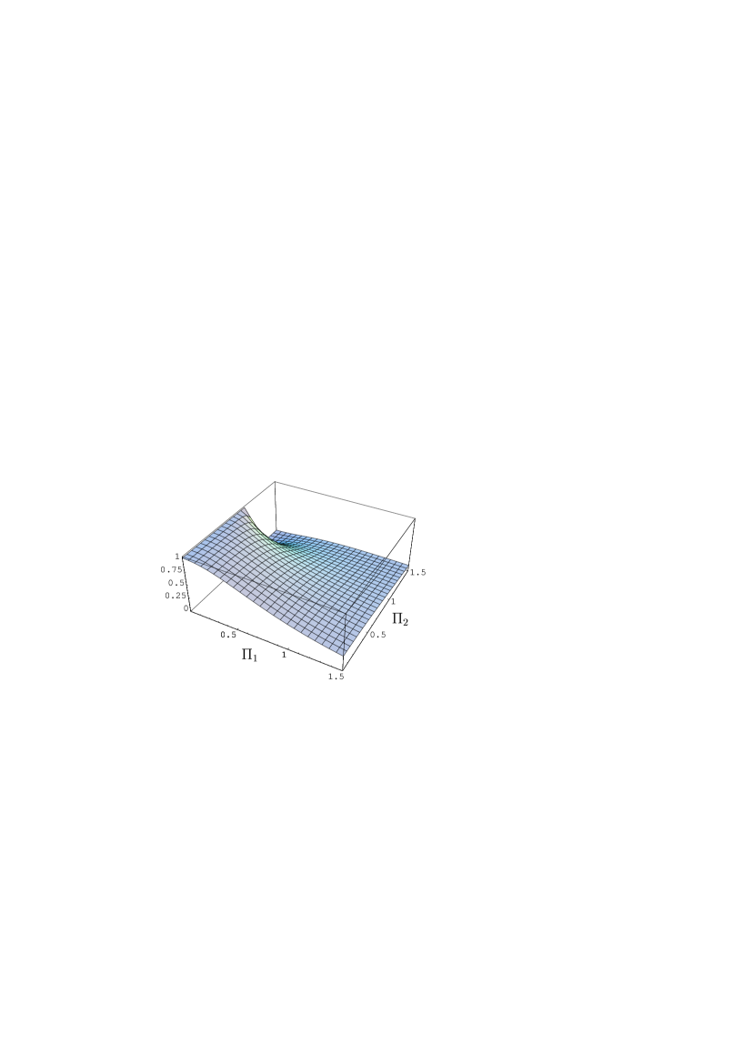
Figure 1: (Color online) The quantity $|\beta_{\mbox{\scriptsize\boldmath$\Pi$}}|^{2}$ as a function of $\Pi_{1}$ and $\Pi_{2}$ is plotted for the single pulse of an electric field (57) satisfying the condition $\pi v_{F}eE_{0}/(\hbar\Omega^{2})<1$.

The characteristic behavior of the quantity $|\beta_{\mbox{\scriptsize\boldmath$\Pi$}}|^{2}$ as a function of $\Pi_{1}$ and $\Pi_{2}$ is different for different values of field parameters $E_{0}$ and $\Omega$. We start from the region of parameters satisfying the condition $\theta<1$, where $\theta$ is defined in Eq. (59). The typical image of the function $|\beta_{\mbox{\scriptsize\boldmath$\Pi$}}|^{2}$ in this case is shown in Fig. 1 for $\theta=0.48$. This corresponds, e.g., to $\Omega=10^{12}\,\mbox{s}^{-1}$ and $E_{0}=1\,$V/cm or $\Omega=10^{13}\,\mbox{s}^{-1}$ and $E_{0}=100\,$V/cm. Under the condition $\theta<1$ Eq. (65) is satisfied with sufficient accuracy, so that integrations in Eq. (63) can be performed up to $\infty$. To gain a better understanding of different parameter regions, in Table I we list the typical values of $E_{0}$ and $\Omega$ and respective values of our parameters $\theta$ and $\Pi_{\max}$ (the latter is presented only for the case $\theta>1$, see below).

The characteristic feature seen in Fig. 1 is the break of continuity of the function $|\beta_{\mbox{\scriptsize\boldmath$\Pi$}}|^{2}$ at $\Pi_{1}=0$, $\Pi_{2}=1$. This is the general property which holds at any $\theta$ and can be easily understood analytically. From Eq. (62) it follows that at $\Pi_{1}=0$

$$\tilde{\kappa}_{+}=\left\{\mbox{\begin{tabular}[]{l}$1-\Pi_{2},{\ }\Pi_{2}\leq 1,$\\ $\Pi_{2}-1,{\ }\Pi_{2}>1,$\end{tabular}}\right.\quad\tilde{\kappa}_{-}=\Pi_{2}+1.$$ (66)

Then the combinations entering Eq. (64) are given by

$$1-\frac{\tilde{\kappa}_{+}-\tilde{\kappa}_{-}}{2}=\left\{\mbox{\begin{tabular}[]{l}$1+\Pi_{2}=\tilde{\kappa}_{-},{\ \ }\Pi_{2}\leq 1,$\\ $2,{\ \ }\Pi_{2}>1,$\end{tabular}}\right.$$ (69)

(70)

$$1+\frac{\tilde{\kappa}_{+}-\tilde{\kappa}_{-}}{2}=\left\{\mbox{\begin{tabular}[]{l}$1-\Pi_{2}=\tilde{\kappa}_{+},{\ \ }\Pi_{2}\leq 1,$\\ $0,{\ \ }\Pi_{2}>1.$\end{tabular}}\right.$$ (73)

Substituting Eq. (70) in Eq. (64), one obtains

$$|\beta_{\mbox{\scriptsize\boldmath$\Pi$}}|^{2}=\left\{\mbox{\begin{tabular}[]{l}$1,{\quad}\Pi_{2}\leq 1,$\\ $0,{\quad}\Pi_{2}>1,$\end{tabular}}\right.$$ (74)

i.e., there is a break of continuity at $\Pi_{2}=1$.

It is convenient to perform integration in Eq. (63) in the polar coordinates $\Pi_{1}=\Pi\cos\varphi$, $\Pi_{2}=\Pi\sin\varphi$ and consider separately the regions of integration $\Pi\leq 1$ and $\Pi\geq 1$. Then Eq. (63) can be rearranged to the form

$$n_{\rm tot}=\frac{4}{\pi^{2}}\left(\frac{eE_{0}}{\hbar\Omega}\right)^{2}Y,$$ (75)

$$Y=\int_{0}^{\pi/2}\!\!\!\!d\varphi\left(\int_{0}^{1}\!\!\!\!\Pi d\Pi|\beta_{\mbox{\scriptsize\boldmath$\Pi$}}|^{2}+\int_{1}^{\infty}\!\!\!\!\Pi d\Pi|\beta_{\mbox{\scriptsize\boldmath$\Pi$}}|^{2}\right)\equiv Y_{1}+Y_{2},$$

where $|\beta_{\mbox{\scriptsize\boldmath$\Pi$}}|^{2}$ is given in Eq. (64). Numerical evaluation of the integral $Y_{1}$ shows that it depends only weakly on the parameter $\theta$. Thus, for $\theta\geq 0.99$ it holds $Y_{1}=0.56$, for $\theta=0.48$ and $\theta\leq 0.048$ we find $Y_{1}=0.59$ and $Y_{1}=0.60$, respectively. This integral can be also estimated analytically taking into account that for $\theta\ll 1$ and $\Pi\ll 1$ the hyperbolic functions in Eq. (64) can be replaced with their arguments

$$Y_{1}\approx\int_{0}^{\pi/2}\!\!\!\!d\varphi\int_{0}^{1}\!\!\!\!\Pi d\Pi\frac{4-(\tilde{\kappa}_{+}-\tilde{\kappa}_{-})^{2}}{4\tilde{\kappa}_{+}\tilde{\kappa}_{-}}$$

$$~{}~{}~{}~{}=\frac{1}{2}\int_{0}^{\pi/2}\!\!\!\!d\varphi\int_{0}^{1}\!\!\!\!\Pi d\Pi\left(1+\frac{1-\Pi^{2}}{\tilde{\kappa}_{+}\tilde{\kappa}_{-}}\right).$$ (76)

Expanding the last expression in powers of $\Pi$, we find

$$Y_{1}\approx\int_{0}^{\pi/2}\!\!\!\!d\varphi\int_{0}^{1}\!\!\!\!\Pi d\Pi\left(1-\frac{1}{2}\Pi^{2}\right)=\frac{3\pi}{16}=0.589$$ (77)

in a very good agreement with the results of numerical computations. Thus, in fact our analytic result is applicable in a wider region of parameters $\theta<1$.

In the region $\Pi>1$ the numerical evaluation of the integral $Y_{2}$ for $\theta=0.48$, 0.048, $4.8\times 10^{-3}$, and $4.8\times 10^{-4}$ leads to $Y_{2}=0.831$, 2.57, 4.38, and 6.19, respectively. On the other hand, for $\theta\ll 1$ and $\Pi\gg 1$ one can replace the hyperbolic sines with their arguments in the numerator of Eq. (64) (using the fact that the large quantity $\Pi$ is canceled) and put $\tilde{\kappa}_{+}\approx\tilde{\kappa}_{-}\approx\Pi$ in the denominator. Then we arrive at

$$Y_{2}\approx\int_{0}^{\pi/2}\!\!\!\!d\varphi\int_{1}^{\infty}\!\!\!\!\Pi d\Pi\frac{\theta^{2}(1-\sin^{2}\varphi)}{\sinh^{2}(\theta\Pi)}=\frac{\pi}{4}\int_{\theta}^{\infty}\!\!d\eta\frac{\eta}{\sinh^{2}\eta}$$

$$~{}~{}=\frac{\pi}{4}(-\ln 2+\theta\coth\theta-\ln\sinh\theta)\approx\frac{\pi}{4}\left[1-\ln(2\theta)\right].$$ (78)

For the same values of $\theta$, as indicated above, the analytic expression (78) results in the following respective values: $Y_{2}=0.817$, 2.62, 4.43, and 6.24. Thus, in fact our asymptotic expression (78) works good in a much wider region $\theta<1$.

By adding Eqs. (77) and (78) in accordance with Eq. (75), we obtain

$$Y=\frac{\pi}{4}\left[\frac{7}{4}-\ln(2\theta)\right].$$ (79)

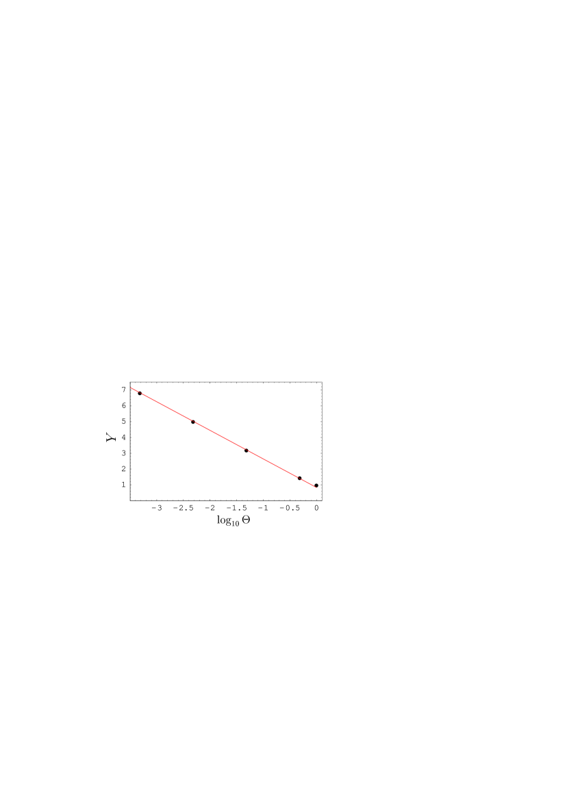
Figure 2: (Color online) The computational results for the quantity $Y$ defined in Eq. (75) as a function of $\theta=\pi v_{F}eE_{0}/(\hbar\Omega^{2})$ are shown as bold dots. The analytical dependence of $Y$ on $\theta$ from Eq. (79) is plotted by the solid line.

In Fig. 2 the values of $Y$ are shown by the solid line as a function of $\log_{10}\theta$. In the same figure the results of numerical computations are indicated by dots. It is seen that simple analytic expression (79) is in a very good agreement with our computational results over a wide region of parameters. Substituting Eq. (79) in Eq. (75), for the total number of graphene quasiparticles per unit area created by the electric field (57) under the condition $\theta<1$, we arrive at the following result:

$$n_{\rm tot}=\frac{1}{\pi}\left(\frac{eE_{0}}{\hbar\Omega}\right)^{2}\left[\frac{7}{4}-\ln\left(\frac{2\pi v_{F}eE_{0}}{\hbar\Omega^{2}}\right)\right].$$ (80)

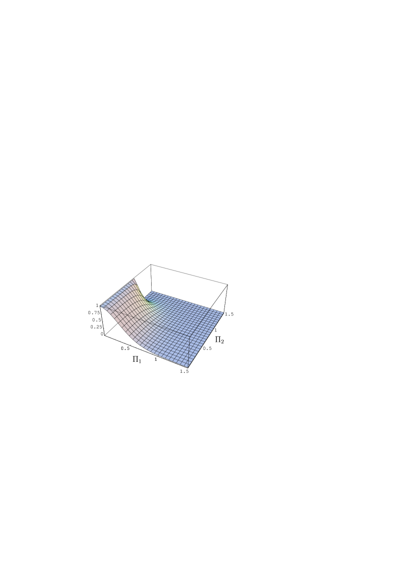
Figure 3: (Color online) The quantity $|\beta_{\mbox{\scriptsize\boldmath$\Pi$}}|^{2}$ as a function of $\Pi_{1}$ and $\Pi_{2}$ is plotted for the single pulse of an electric field (57) satisfying the condition $\pi v_{F}eE_{0}/(\hbar\Omega^{2})>1$.

We now turn our attention to the case $\theta>1$. In this case the characteristic behavior of $|\beta_{\mbox{\scriptsize\boldmath$\Pi$}}|^{2}$ as a function of $\Pi_{1}$ and $\Pi_{2}$ is shown in Fig. 3 plotted for $\theta=4.8$. As is seen in Fig. 3, for $\theta>1$ the surface representing $|\beta_{\mbox{\scriptsize\boldmath$\Pi$}}|^{2}$ is more concentrated around the coordinate origin than in the case $\theta<1$. With further increase of $\theta$ the region in a $(\Pi_{1},\Pi_{2})$-plane, giving major contribution to the integral (63), quickly decreases. The integration in Eq. (63) can be performed analytically under the condition $\theta\gg 1$. In this case the hyperbolic functions in Eq. (64) can be replaced with the exponents and we arrive at

$$|\beta_{\mbox{\scriptsize\boldmath$\Pi$}}|^{2}\approx e^{\theta(2-\tilde{\kappa}_{+}-\tilde{\kappa}_{-})}.$$ (81)

Unlike the case $\theta<1$, considered above, in the case $\theta>1$ the region of integration in Eq. (63) requires more caution. Thus, if $\Pi_{\max}\leq 1$ (i.e., $eE_{0}/\Omega\geq p_{\max}$), where $\Pi_{\max}$ from Eq. (65) is the maximum dimensionless momentum allowed by the Dirac model, the contributing momentum $\Pi$ might be larger than $\Pi_{\max}$. Then the integration in Eq. (63) must be performed up to $\Pi_{\max}$ in order do not go beyond the scope of the Dirac model. In this case we can put

$$2-\tilde{\kappa}_{+}-\tilde{\kappa}_{-}\approx-\cos^{2}\!\varphi\,\Pi^{2}$$ (82)

and Eq. (63) leads to

$$n_{\rm tot}\approx\frac{4}{\pi^{2}}\left(\frac{eE_{0}}{\hbar\Omega}\right)^{2}\int_{0}^{\pi/2}\!\!\!\!d\varphi\int_{0}^{\Pi_{\max}}\!\!\!\!\Pi d\Pi e^{-\theta\cos^{2}\!\varphi\Pi^{2}}$$

$$~{}~{}=\frac{\Pi_{\max}^{2}}{\pi}\left(\frac{eE_{0}}{\hbar\Omega}\right)^{2}\,e^{-\theta\Pi_{\max}^{2}/2}$$ (83)

$$~{}~{}~{}~{}~{}~{}~{}~{}~{}\times\left[I_{0}\left(\frac{\theta\Pi_{\max}^{2}}{2}\right)+I_{1}\left(\frac{\theta\Pi_{\max}^{2}}{2}\right)\right],$$

where $I_{n}(z)$ are the Bessel functions of imaginary argument. Keeping in mind the condition $\theta\Pi_{\max}^{2}\gg 1$, which is satisfied in our case, and using the asymptotic expressions for the Bessel functions at large arguments, we obtain a more simple expression

$$n_{\rm tot}\approx\frac{2}{\pi^{2}}\frac{p_{m}}{\hbar}\sqrt{\frac{eE_{0}}{\hbar v_{F}}}.$$ (84)

This gives the lower limit for the number of created pairs per unit area of graphene under the condition $\Pi_{\max}\leq 1$, i.e., $eE_{0}/\Omega\geq p_{\max}$. It is interesting to note that the result in this case does not depend on $\Omega$, i.e., on the lifetime of the field [see Table I for the region of $E_{0}$ and $\Omega$ where Eq. (84) is applicable].

Another option which can be realized in the case $\theta>1$ is $\Pi_{\max}>1$, i.e., $eE_{0}/\Omega<p_{\max}$. Under these conditions Eq. (65) is satisfied for all contributing momenta, so that the integration in Eq. (63) can be performed up to infinity. To calculate the integral we again represent the quantity (63) in the form (75). Then the contribution $Y_{1}$ can be calculated according to Eq. (83) with the upper integration limit $\Pi_{\max}$ replaced with unity. This leads to

$$Y_{1}\approx\frac{\sqrt{\pi}}{2\sqrt{\theta}}=\frac{\sqrt{\hbar}\Omega}{2\sqrt{v_{F}eE_{0}}}.$$ (85)

In the region $\Pi>1$ it holds $\tilde{\kappa}_{+}+\tilde{\kappa}_{-}\approx 2\Pi$ and with account of Eq. (81) the contribution $Y_{2}$ is the following

$$Y_{2}\approx\int_{0}^{\pi/2}\!\!\!\!d\varphi\int_{1}^{\infty}\!\!\!\!\Pi d\Pi e^{2\theta(1-\Pi)}=\frac{\pi}{4\theta}\left(1+\frac{1}{2\theta}\right)$$

$$~{}~{}~{}~{}\approx\frac{\pi}{4\theta}=\frac{\hbar\Omega^{2}}{4v_{F}eE_{0}}.$$ (86)

Substituting Eqs. (85) and (86) in Eq. (75), for the total number of pairs per unit area, created in the case $\theta\gg 1$ and $eE_{0}/\Omega<p_{\max}$, we obtain

$$n_{\rm tot}\approx\frac{2}{\pi^{2}}\frac{(eE_{0})^{3/2}}{\hbar^{3/2}v_{F}^{1/2}\Omega}\left[1+\frac{\hbar^{1/2}\Omega}{2(v_{F}eE_{0})^{1/2}}\right].$$ (87)

By contrast with Eq. (84), here the number of created pairs depends on a lifetime of the electric field [the region of $E_{0}$ and $\Omega$ where Eq. (87) is applicable can be seen in Table I]. We note also that although Eq. (87) was derived under the condition $\theta\gg 1$, it is in fact applicable starting from $\theta\approx 2$ due to the specific functional form of $|\beta_{\mbox{\scriptsize\boldmath$\Pi$}}|^{2}$.

V Comparison with the case of static electric field

As discussed in Sec. I, the creation of quasiparticles in graphene by the space homogeneous static electric field was investigated in Refs. 22 ; 29 . Here we reproduce the results of these references as a limiting case of the time-dependent field considered in Sec. IV and compare the numbers of pairs created by the static and time-dependent fields.

The static space homogeneous electric field directed along the axis $x^{2}$ can be obtained as a particular case of the time-dependent field (57) when $\Omega\to 0$

$$A^{2}=-E_{0}ct,\qquad E^{2}=E_{0}.$$ (88)

The spectral density of pairs created by the constant field can be found by the limiting transition $\Omega\to 0$ in the spectral density (60). For this purpose, using the expressions for $\kappa_{\pm}$ in Eq. (59), we find that at small $\Omega$

$$\kappa_{\pm}\approx\frac{eE_{0}}{\Omega}\mp p_{2}+\frac{p_{1}^{2}}{2}\,\frac{\Omega}{eE_{0}}.$$ (89)

From Eq. (89) one obtains

$$\kappa_{+}-\kappa_{-}\approx-2p_{2}.$$ (90)

With the help of Eq. (90), for the arguments of both hyperbolic sines in the numerator of Eq. (60) we arrive at

$$\theta\mp\frac{\pi v_{F}(\kappa_{+}-\kappa_{-})}{2\hbar\Omega}\approx\frac{\pi v_{F}eE_{0}}{\hbar\Omega^{2}}\pm p_{2}\frac{\pi v_{F}}{\hbar\Omega}.$$ (91)

Now we multiply both sides of Eq. (89) by $\pi v_{F}/(\hbar\Omega)$ and obtain

$$\frac{\pi v_{F}\kappa_{\pm}}{\hbar\Omega}\approx\frac{\pi v_{F}eE_{0}}{\hbar\Omega^{2}}\mp p_{2}\frac{\pi v_{F}}{\hbar\Omega}+\frac{p_{1}^{2}}{2}\,\frac{\pi v_{F}}{\hbar eE_{0}}.$$ (92)

Then, by comparing the right-hand sides of Eqs. (91) and (92), we find

$$\theta\mp\frac{\pi v_{F}(\kappa_{+}-\kappa_{-})}{2\hbar\Omega}\approx\frac{\pi v_{F}\kappa_{\mp}}{\hbar\Omega}-\frac{p_{1}^{2}}{2}\,\frac{\pi v_{F}}{\hbar eE_{0}}.$$ (93)

Taking into account that in the limiting case $\Omega\to 0$ all hyperbolic sines in Eq. (60) can be replaced with the exponents, the final result for a static electric field is

$$|\beta_{\mbox{\scriptsize\boldmath$\Pi$}}|^{2}=e^{-{\pi v_{F}p_{1}^{2}}/({\hbar eE_{0}})}$$ (94)

in agreement with Refs. 22 ; 29 . We note that the right-hand side of Eq. (94) does not depend on $p_{2}$. In this case, as was shown in Ref. 5 for the massive particles in (3+1)-dimensions, the integration with respect to $p_{2}$ in Eq. (56) should be performed according to

$$\int_{-\infty}^{\infty}\!\!\!dp_{2}=eE_{0}T,$$ (95)

where $T$ is the total (infinitely large) lifetime of the static electric field. Substituting Eqs. (94) and (95) in Eq. (56), we obtain

$$n_{\rm tot}=\frac{(eE_{0})^{3/2}}{\pi^{2}\hbar^{3/2}v_{F}^{1/2}}T.$$ (96)

In the case of a static field the physically meaningful quantity is not $n_{\rm tot}$, but the number of pairs created per unit area of graphene per unit time

$$I_{\rm tot}=\frac{n_{\rm tot}}{T}=\frac{(eE_{0})^{3/2}}{\pi^{2}\hbar^{3/2}v_{F}^{1/2}},$$ (97)

which is also called the local rate of pair creation 22 .

The results (96) and (97) were derived without regard for the application range of the Dirac model in Eq. (65). In fact the integration with respect to $p_{1}$ satisfies the condition (65) with large safety margin, whereas the integration with respect to $p_{2}$ does not. If we wish to stay within the application region of the Dirac model, Eq. (95) should be replaced with

$$\int_{-p_{\max}}^{p_{\max}}\!\!\!dp_{2}=2p_{\max}.$$ (98)

As a result, the lower limit for the number of pairs created by the static field during its infinitely long lifetime is given by

$$n_{\rm tot}=\frac{2}{\pi}\frac{p_{m}}{\hbar}\sqrt{\frac{eE_{0}}{\hbar v_{F}}}.$$ (99)

This coincides with Eq. (84) obtained for the time-dependent field (88) satisfying the conditions $\theta>1$ and $\Pi_{\max}<1$, as it should be.

It is interesting to formally compare the creation rate by the static field (97) with respective results for the time-dependent field (57). First we consider the case $\theta>1$ and $\Pi_{\max}>1$ when the total number of created pairs per unit area of graphene is given by Eq. (87). For a lifetime of the field (57) one can take the time interval $T=4/\Omega$ during which this field increases from $0.07E_{0}$ to $E_{0}$ and then decreases back to $0.07E_{0}$. The mean value of the field (57) during this lifetime is given by

$$\bar{E}=\frac{1}{T}\int_{-T/2}^{T/2}\frac{E_{0}\,dt}{\cosh^{2}(\Omega t)}=\frac{E_{0}}{2}\frac{e^{4}-1}{e^{4}+1}\approx\frac{E_{0}}{2}$$ (100)

and the mean creation rate is obtained from Eq. (87) with $\Omega=4/T$

$$\bar{I}_{\rm tot}=\frac{n_{\rm tot}}{T}=\frac{1}{2\pi^{2}}\,\frac{(eE_{0})^{3/2}}{\hbar^{3/2}v_{F}^{1/2}}$$ (101)

[we consider the values of parameters where it is possible to omit the second term on the right-hand side of Eq. (87); see below for full computational results]. This should be compared with the creation rate (97) for a static field having the same strength as the mean strength of a time-dependent field, i.e., with $E_{0}$ replaced for $E_{0}/2$:

$${I}_{\rm tot}=\frac{n_{\rm tot}}{T}=\frac{1}{2\sqrt{2}\pi^{2}}\,\frac{(eE_{0})^{3/2}}{\hbar^{3/2}v_{F}^{1/2}}.$$ (102)

A comparison between the right-hand sides of Eqs. (101) and (102) shows that the creation rate for a time-dependent field is by a factor of 1.41 larger than for a static field.

Using this method of comparison, we now compare the creation rates of graphene quasiparticles, created by the time-dependen and static electric fields, for different values of field parameters. We begin with the case $\theta<1$ when $n_{\rm tot}$ is given by Eq. (80). The creation rates $\bar{I}_{\rm tot}$ calculated for a lifetime $T=4/\Omega$ for $E_{0}=0.1\,$V/cm, $\Omega=10^{12}\,\mbox{s}^{-1}$ ($\theta=4.8\times 10^{-2}$) and $E_{0}=10^{4}\,$V/cm, $\Omega=10^{14}\,\mbox{s}^{-1}$ ($\theta=0.48$) are $7.5\times 10^{15}\,\mbox{cm}^{-2}\mbox{s}^{-1}$ and $3.2\times 10^{23}\,\mbox{cm}^{-2}\mbox{s}^{-1}$, respectively (see Table I). These should be compared with respective creation rates $I_{\rm tot}$ in the static electric field equal to $E_{0}/2$: $6.7\times 10^{15}\,\mbox{cm}^{-2}\mbox{s}^{-1}$ and $2.1\times 10^{23}\,\mbox{cm}^{-2}\mbox{s}^{-1}$. As can be seen from the comparison, the creation rates by time-dependent fields are larger by the factors 1.12 and 1.52, respectively.

Next, we consider the case $\theta>1$ and $eE_{0}/\Omega<p_{\max}$ where Eq. (87) for $n_{\rm tot}$ is applicable. Here, the creation rates $\bar{I}_{\rm tot}$ calculated for the parameters $E_{0}=0.1\,$V/cm, $\Omega=10^{11}\,\mbox{s}^{-1}$ ($\theta=4.8$, $eE_{0}/\Omega=10^{-4}p_{\max}$) and $E_{0}=10^{3}\,$V/cm, $\Omega=10^{13}\,\mbox{s}^{-1}$ ($\theta=4.8$, $eE_{0}/\Omega=10^{-2}p_{\max}$) are $1.32\times 10^{16}\,\mbox{cm}^{-2}\mbox{s}^{-1}$ and $1.32\times 10^{22}\,\mbox{cm}^{-2}\mbox{s}^{-1}$, respectively (see Table I). These should be compared with respective creation rates $I_{\rm tot}$ in the static electric fields $6.7\times 10^{15}\,\mbox{cm}^{-2}\mbox{s}^{-1}$ and $6.7\times 10^{21}\,\mbox{cm}^{-2}\mbox{s}^{-1}$ leading to an excess by the factor of 1.97 in the case of time-dependent fields. Note that the factor 1.97 obtained now exceeds the factor 1.41 obtained above from the comparison of Eq. (101) valid in the region $\theta<1$ and $eE_{0}/\Omega<p_{\max}$ and Eq. (102). This is because for the field parameters chosen now the second term on the right-hand side of Eqs. (87) contributes significantly. The values of the field parameters leading to the factor 1.41 are illustrated below.

As the last example, we consider the field parameters satisfying the conditions $\theta>1$ and $eE_{0}/\Omega\geq p_{\max}$, i.e., the application region of Eq. (84). In this region, in accordance to Table I, we take the following values of parameters: $E_{0}=1\,$V/cm, $\Omega=10^{8}\,\mbox{s}^{-1}$ ($\theta=4.8\times 10^{7}$, $eE_{0}/\Omega=p_{\max}$) and $E_{0}=10^{4}\,$V/cm, $\Omega=10^{11}\,\mbox{s}^{-1}$ ($\theta=4.8\times 10^{5}$, $eE_{0}/\Omega=10p_{\max}$). Then we get $\bar{I}_{\rm tot}=3\times 10^{17}\,\mbox{cm}^{-2}\mbox{s}^{-1}$ and $\bar{I}_{\rm tot}=3\times 10^{22}\,\mbox{cm}^{-2}\mbox{s}^{-1}$, respectively. Comparing with respective values in the case of a static field (${I}_{\rm tot}=2.1\times 10^{17}\,\mbox{cm}^{-2}\mbox{s}^{-1}$ and ${I}_{\rm tot}=2.1\times 10^{23}\,\mbox{cm}^{-2}\mbox{s}^{-1}$), we find that for the first set of field parameters there is an excess by the factor 1.42 in the case of a time-dependent field. This is because these field parameters satisfy a condition $eE_{0}/\Omega=p_{\max}$ on the borderline to $eE_{0}/\Omega<p_{\max}$ where Eq. (87) with neglected second term on the right-hand side is applicable (in so doing the value of $\theta$ has a little effect; it is only required that $\theta\gg 1$). As to the second set of field parameters, the number of pairs created by a static field is seven times larger than by a time-dependent field.

In the above computations we did not take into account the back reaction of created pairs on an external field. For a static field an estimation of the time interval after which the effect of back reaction should be taken into account is provided in Ref. 22 . Keeping in mind that according to our computations the creation rates in static and time-dependent fields are qualitatively the same, this estimation is applicable in our case as well.

VI Conclusions and discussion

In the foregoing we have investigated the creation of quasiparticle pairs in graphene by the space homogeneous time-dependent electric field. For this purpose the previously developed formalism describing the creation of electron-positron pairs by a nonstationary field in (3+1)-dimensional case was adapted for massless particles in (2+1)-dimensional space-time. This allowed to express the characteristics of created pairs via the asymptotic solutions at $t\to\infty$ of the second-order ordinary differential equation of an oscillator type with complex frequency.

The fundamental difference with the case of massive particles, whose creation is exponentially suppressed for fields below $10^{16}\,$V/cm, is that the creation of massless quasiparticles in graphene occurs in easily accessible weak fields 22 ; 29 . This presents unique opportunity to test the nonlinear effects of quantum electrodynamics, such as particle creation from vacuum by an external field, on a laboratory table with no use of huge concentrations of energy and related expensive setups. In this regard it should be noted that another prediction of quantum electrodynamics, the Casimir effect, is already widely discussed in application to graphene (see, e.g., Refs. 34 ; 35 ; 36 ; 37 ; 38 ; 39 ), and the measurement of the Casimir force from graphene sheet has been performed very recently 40 . At the moment graphene single crystals with dimensions of up to $500\,\mu$m on a side and electron mobility higher than $4000\,\mbox{cm}^{2}\,\mbox{V}^{-1}\,\mbox{s}^{-1}$ (i.e., $\sim 10^{10}\,\mbox{cm}^{-2}$ concentration of impurities) are obtained 41 . This is more favorable for observation of the effect of pair creation than the parameters used in Ref. 22 ($100\,\mu$m and $2\times 10^{11}\,\mbox{cm}^{-2}$, respectively).

The creation of graphene quasiparticles by a time-dependent electric field, considered in this paper, may present some advantages with respect to the experimental observation, as compared to the case of static field. It presents a wide variety of different creation regimes depending on the field parameters. All these regimes are considered in our paper in detail, and simple analytic expressions for the number of created pairs per unit area of graphene convenient for applications are obtained in each case. For this purpose the exact solution of Dirac equation describing the interaction of quasiparticles with a single pulse of electric field has been used. Special attention was paid to the cases when the creation rate in a time-dependent field is larger than in a static field.

In future it would be interesting to investigate the creation of quasiparticle pairs in graphene by electromagnetic fields of more complicated configurations, specifically, by the electric field with periodic dependence on time.

         

         

         

Table 1: The values of parameters $\theta$ and $\Pi_{\max}$ determining the applicability of Eqs. (80), (84) or (87) for the number of created pairs per unit area of graphene for different field strengths $E_{0}$ and different $\Omega$.

$E_{0}$	$\Omega\,(\mbox{s}^{-1})$
(V/cm)	$10^{8}$	$10^{11}$	$10^{12}$	$10^{13}$	$10^{14}$
0.1	$\theta=4.8\times 10^{6}$	$\theta=4.8$	$\theta=4.8\times 10^{-2}$	$\theta=4.8\times 10^{-4}$	$\theta=4.8\times 10^{-6}$
	$\Pi_{\max}=10$	$\Pi_{\max}=10^{4}$
1	$\theta=4.8\times 10^{7}$	$\theta=48$	$\theta=0.48$	$\theta=4.8\times 10^{-3}$	$\theta=4.8\times 10^{-5}$
	$\Pi_{\max}=1$	$\Pi_{\max}=10^{3}$
$10^{3}$	$\theta=4.8\times 10^{10}$	$\theta=4.8\times 10^{4}$	$\theta=4.8\times 10^{2}$	$\theta=4.8$	$\theta=4.8\times 10^{-2}$
	$\Pi_{\max}=10^{-3}$	$\Pi_{\max}=1$	$\Pi_{\max}=10$	$\Pi_{\max}=100$
$10^{4}$	$\theta=4.8\times 10^{11}$	$\theta=4.8\times 10^{5}$	$\theta=4.8\times 10^{3}$	$\theta=48$	$\theta=0.48$
	$\Pi_{\max}=10^{-4}$	$\Pi_{\max}=0.1$	$\Pi_{\max}=1$	$\Pi_{\max}=10$