Adaptive confidence intervals for regression functions under shape constraints

Abstract

Adaptive confidence intervals for regression functions are constructed under shape constraints of monotonicity and convexity. A natural benchmark is established for the minimum expected length of confidence intervals at a given function in terms of an analytic quantity, the local modulus of continuity. This bound depends not only on the function but also the assumed function class. These benchmarks show that the constructed confidence intervals have near minimum expected length for each individual function, while maintaining a given coverage probability for functions within the class. Such adaptivity is much stronger than adaptive minimaxity over a collection of large parameter spaces.

, and t2Supported in part by NSF FRG Grant DMS-08-54973.

1 Introduction

The construction of useful confidence sets is one of the more challenging problems in nonparametric function estimation. There are two main interrelated issues which need to be considered together, coverage probability and the expected size of the confidence set. For a fixed parameter space it is often possible to construct confidence sets which have guaranteed coverage probability over the parameter space while controlling the maximum expected size. However such minimax statements are often thought to be too conservative, and a more natural goal is to have the expected size of the confidence set reflect in some sense the difficulty of estimating the particular underlying function.

These issues are well illustrated by considering confidence intervals for the value of a function at a fixed point. Let $Y$ be an observation from the white noise model

$$dY(t)=f(t)\,dt+n^{-{1}/{2}}\,dW(t),\qquad-\tfrac{1}{2}\leq t\leq\tfrac{1}{2},$$ (1)

where $W(t)$ is standard Brownian motion and $f$ belongs to some parameter space ${{\mathcal{F}}}$. Suppose that we wish to construct a confidence interval for $f$ at some point $t_{0}\in(-\frac{1}{2},\frac{1}{2})$. Let $\mathrm{CI}$ be a confidence interval for $f(t_{0})$ based on observing the process $Y$, and let $L(\mathrm{CI})$ denote the length of the confidence interval. The minimax point of view can then be expressed by the following: subject to the constraint on the coverage probability $\inf_{f\in{\mathcal{F}}}P(f(t_{0})\in\mathrm{CI})\geq 1-\alpha$, minimize the maximum expected length $\sup_{f\in{\mathcal{F}}}E_{f}(L(\mathrm{CI}))$.

As an example it is common to consider the Lipschitz classes

$$\Lambda(\beta,M)=\bigl{\{}f\dvtx\bigl{|}f(y)-f(x)\bigr{|}\leq M|y-x|^{\beta}\mbox{ for $x,y\in\bigl{[}-\tfrac{1}{2},\tfrac{1}{2}\bigr{]}$}\bigr{\}},\qquad\mbox{if $0<\beta\leq 1$}$$

and for $\beta>1$

$$\Lambda(\beta,M)=\bigl{\{}f\dvtx\bigl{|}f^{(\lfloor\beta\rfloor)}(x)-f^{(\lfloor\beta\rfloor)}(y)\bigr{|}\leq M|x-y|^{\beta^{\prime}}\mbox{ for $x,y\in\bigl{[}-\tfrac{1}{2},\tfrac{1}{2}\bigr{]}$}\bigr{\}},$$

where $\lfloor\beta\rfloor$ is the largest integer less than $\beta$ and $\beta^{\prime}=\beta-\lfloor\beta\rfloor$. For these classes it easily follows from results of Donoho (1994), Low (1997) and Evans, Hansen and Stark (2005) that the minimax expected length of confidence intervals, which have guaranteed coverage of $1-\alpha$ over $\Lambda(\beta,M)$, is of order $M^{1/(1+2\beta)}n^{-{\beta/(1+2\beta)}}$.

It should, however, be stressed that confidence intervals which achieve such an expected length rely on the knowledge of the particular smoothness parameters $\beta$ and $M$, which are not known in most applications. Unfortunately, Low (1997) and Cai and Low (2004) have shown that the natural goal of constructing an adaptive confidence interval which has a given coverage probability and has expected length that is simultaneously close to these minimax expected lengths for a range of smoothness parameters is not in general attainable. More specifically suppose that a confidence interval has guaranteed coverage probability of $1-\alpha$ over $\Lambda(\beta,M)$. Then for any $f$ in the interior of $\Lambda(\beta,M)$ the expected length for this $f$ must also be of order $n^{-{\beta/(1+2\beta)}}$. In other words the minimax rate describes the actual rate for all functions in the class other than those on the boundary of the set. For example, in the case that a confidence interval has guaranteed coverage probability of $1-\alpha$ over the Lipschitz class $\Lambda(1,M)$, then even if the underlying function has two derivatives, and the first derivative smaller than $M$, the confidence interval for $f(x)$ must still have expected length of order $n^{-1/3}$ even though one would hope that an adaptive confidence interval would have a much shorter length of order $n^{-2/5}$.

Despite these very negative results there are some settings where some degree of adaptation has been shown to be possible. In particular under certain shape constraints Hengartner and Stark (1995) constructed confidence bands which have a guaranteed coverage probability of at least $1-\alpha$ over the collection of all monotone densities and which have maximum expected length of order $(\frac{\log n}{n})^{\beta/(2\beta+1)}$ for those monotone densities which are in $\Lambda(\beta,M)$ for a particular choice of $\beta$ where $0<\beta\leq 1$. This construction relies on the selection of a tuning parameter and is thus not adaptive. Dümbgen (2003), however, does provide adaptive confidence bands with optimal rates for both isotonic and convex functions under supremum norm loss on arbitrary compact subintervals. These results are, however, still framed in terms of the maximum length over particular large parameter spaces, and the existence of such intervals raises the question of exactly how much adaption is possible. It is this question that is the focus of the present paper.

Rather than considering the maximum expected length over large collections of functions, we study the problem of adaptation to each and every function in the parameter space. We examine this problem in detail for two commonly used collections of functions that have shape constraints, namely the collection of convex functions and the collection of monotone functions. We focus on these parameter spaces as it is for such shape constrained problems for which there is some hope for adaptation. Within this context we consider the problem of constructing a confidence interval for the value of a function at a fixed point under both the white noise with drift model given in (1) as well as a nonparametric regression model. We show that within the class of convex functions and the class of monotone functions, it is indeed possible to adapt to each individual function, and not just to the minimax expected length over different parameter spaces in a collection. The notion of adaptivity to a single function is also discussed in Lepski, Mammen and Spokoiny (1997) and Lepski and Spokoiny (1997) for the related point estimation problem but in these contexts a logarithmic penalty of the noise level must be paid, and thus the notion of adaptivity is somewhat different.

This result is achieved in two steps. First we study the problem of minimizing the expected length of a confidence interval, assuming that the data is generated from a particular function $f$ in the parameter space, subject to the constraint that the confidence interval has guaranteed coverage probability over the entire parameter space. The solution to this problem gives a benchmark for the expected length which depends on the function $f$ considered. It gives a bound on the expected length of any adaptive interval because if the expected length is smaller than this bound for any particular function, the confidence interval cannot have the desired coverage probability. In applications it is more useful to express the benchmark in terms of a local modulus of continuity, an analytic quantity that can be easily calculated for individual functions. In situations where adaptation is not possible, this local modulus of continuity does not vary significantly from function to function. Such is the case in the settings considered in Low (1997). However, in the context of convex or monotone functions, the resulting benchmark does vary significantly, and this opens up the possibility for adaptation in those settings.

Our second step is to actually construct adaptive confidence intervals. This is done separately for monotone functions and convex functions, with similar results. For example, an adaptive confidence interval is constructed which is shown to have expected length uniformly within an absolute constant factor of the benchmark for every convex function, while maintaining coverage probability over the collection of all convex functions. In other words, this confidence interval has smallest expected length, up to a universal constant factor, for each and every convex function within the class of all confidence intervals which guarantee a $1-\alpha$ coverage probability over all convex functions. A similar result is established for a confidence interval designed for monotone functions.

The rest of the paper is organized as follows. In Section 2 the benchmark for the expected length at each monotone function or each convex function is established under the constraint that the interval has a given level of coverage probability over the collection of monotone functions or the collection of convex functions. Section 3 constructs data driven confidence intervals for both monotone functions and convex functions and shows that these confidence intervals maintain coverage probability and have expected length within an absolute constant factor of the benchmark given in Section 2 for each monotone function and convex function. Section 4 considers the nonparametric regression model, and Section 5 discusses connections of our results with other work in the literature. Proofs are given in Section 6.

2 Benchmark and lower bound on expected length

As mentioned in the Introduction, the focus in this paper is the construction of confidence intervals which have expected length that adapts to the unknown function. The evaluation of these procedures depends on lower bounds which are given here in terms of a local modulus of continuity first introduced by Cai and Low (2011) in the context of point estimation of convex functions under mean squared error loss. These lower bounds provide a natural benchmark for our problems.

2.1 Benchmark and lower bound

We focus in this paper on estimating the function $f$ at $0$ since estimation at other points away from the boundary is similar. For a given function class ${\mathcal{F}}$, write ${\mathcal{I}}_{\alpha}({\mathcal{F}})$ for the collection of all confidence intervals which cover $f(0)$ with guaranteed coverage probability of $1-\alpha$ for all functions in ${\mathcal{F}}$. For a given confidence interval $\mathrm{CI}$, denote by $L(\mathrm{CI})$ the length of $\mathrm{CI}$ and $L(\mathrm{CI},f)=E_{f}(L(\mathrm{CI}))$ the expected length of $\mathrm{CI}$ at a given function $f$. The minimum expected length at $f$ of all confidence intervals with guaranteed coverage probability of $1-\alpha$ over ${\mathcal{F}}$ is then given by

$$L_{\alpha}^{*}(f,{\mathcal{F}})=\inf_{\mathrm{CI}\in{\mathcal{I}}_{\alpha}({\mathcal{F}})}L(\mathrm{CI},f).$$ (2)

A natural goal is to construct a confidence interval with expected length close to the minimum $L_{\alpha}^{*}(f,{\mathcal{F}})$ for every $f\in{\mathcal{F}}$ while maintaining the coverage probability over ${\mathcal{F}}$. However although $L_{\alpha}^{*}(f,{\mathcal{F}})$ is a natural benchmark for the expected length of confidence intervals, it is not easy to evaluate exactly. Instead as a first step toward our goal, we provide a lower bound for the benchmark $L_{\alpha}^{*}(f,{\mathcal{F}})$ in terms of a local modulus of continuity $\omega(\varepsilon,f,{\mathcal{F}})$ introduced by Cai and Low (2011). The local modulus is a quantity that is more easily computable and techniques for its analysis are similar to those given in Donoho and Liu (1991) and Donoho (1994) where a global modulus of continuity was introduced in the study of minimax theory for estimating linear functionals. See the examples in Section 2.2.

For a parameter space $\mathcal{F}$ and function $f\in\mathcal{F}$, the local modulus of continuity is defined by

$$\omega(\varepsilon,f,{\mathcal{F}})=\sup\bigl{\{}\bigl{|}g(0)-f(0)\bigr{|}\dvtx\|g-f\|_{2}\leq\varepsilon,g\in{\mathcal{F}}\bigr{\}},$$ (3)

where $\|\cdot\|_{2}$ is the $L_{2}(-\frac{1}{2},\frac{1}{2})$ function norm. The following theorem gives a lower bound for the minimum expected length $L_{\alpha}^{*}(f,{\mathcal{F}})$ in terms of the local modulus of continuity $\omega(\varepsilon,f,{\mathcal{F}})$. In this theorem and throughout the paper we write $\Phi$ for the cumulative distribution function and $\phi$ for the density function of a standard normal density and set $z_{\alpha}=\Phi^{-1}(1-\alpha)$.

Theorem 1

Suppose ${\mathcal{F}}$ is a nonempty convex set. Let $0<\alpha<{1\over 2}$ and $f\in{\mathcal{F}}$. Then for confidence intervals based on (1),

$$L^{*}_{\alpha}(f,{\mathcal{F}})\geq\biggl{(}1-\frac{1}{\sqrt{2\pi}z_{\alpha}}+\frac{\phi(z_{\alpha})}{z_{\alpha}}-\alpha\biggr{)}\omega\biggl{(}\frac{z_{\alpha}}{\sqrt{n}},f,{\mathcal{F}}\biggr{)}.$$ (4)

In particular,

$$L^{*}_{\alpha}(f,{\mathcal{F}})\geq\biggl{(}1-\frac{1}{\sqrt{2\pi}z_{\alpha}}\biggr{)}\omega\biggl{(}\frac{z_{\alpha}}{\sqrt{n}},f,{\mathcal{F}}\biggr{)}.$$ (5)

The lower bounds given in Theorem 1 can be viewed as benchmarks for the evaluation of the expected length of confidence intervals when the true function is $f$ for confidence intervals which have guaranteed coverage probability over all of ${\mathcal{F}}$. The bound depends on the underlying true function $f$ as well as the parameter space ${\mathcal{F}}$.

The bounds from Theorem 1 are general. In some settings they can be used to rule out the possibility of adaptation, whereas in other settings they provide bounds on how much adaptation is possible. In particular the result ruling out adaptation over Lipschitz classes mentioned in the Introduction easily follows from this theorem. For example, consider the Lipschitz class $\Lambda(\beta,M)$ and suppose that $f$ is in the interior of $\Lambda(\beta,M)$. Straightforward calculations similar to those given in Section 2.2 show that

$$\omega\bigl{(}\varepsilon,f,\Lambda(\beta,M)\bigr{)}\sim C\varepsilon^{2\beta/{(2\beta+1)}}.$$ (6)

Now consider two Lipschitz classes $\Lambda(\beta_{1},M_{1})$ and $\Lambda(\beta_{2},M_{2})$ with $\beta_{1}>\beta_{2}$. A fully adaptive confidence interval in this setting would have guaranteed coverage of $1-\alpha$ over $\Lambda(\beta_{1},M_{1})\cup\Lambda(\beta_{2},M_{2})$ and maximum expected length over $\Lambda(\beta_{i},M_{i})$ of order $n^{\beta_{i}/(2\beta_{i}+1)}$ for $i=1$ and $2$. However, it follows from Theorem 1 and (6) that for all confidence intervals with coverage probability of $1-\alpha$ over $\Lambda(\beta_{2},M_{2})$, for every $f\in\Lambda(\beta_{2},M^{\prime})$ with $M^{\prime}<M_{2}$,

$$L^{*}_{\alpha}\bigl{(}f,\Lambda(\beta_{2},M_{2})\bigr{)}\geq C(\alpha)n^{-{\beta_{2}/(2\beta_{2}+1)}}$$

for some constant $C(\alpha)$ not depending on $f$. In particular this holds for all $f\in\Lambda(\beta_{1},M_{1})\cap\Lambda(\beta_{2},M^{\prime})$ and hence

$$\sup_{f\in\Lambda(\beta_{1},M_{1})}\inf_{\mathrm{CI}\in{\mathcal{I}}_{\alpha}(\Lambda(\beta_{1},M_{1})\cup\Lambda(\beta_{2},M_{2}))}L(\mathrm{CI},f) \geq C(\alpha)n^{-{\beta_{2}/(2\beta_{2}+1)}}$$

$$\gg n^{-{\beta_{1}/(2\beta_{1}+1)}}.$$

Therefore it is not possible to have confidence intervals with adaptive expected length over two Lipschitz classes with different smoothness parameters.

In the present paper Theorem 1 will be used to provide benchmarks in the setting of shape constraints. Denote by $F_{m}$ and $F_{c}$, respectively, the collection of all monotonically nondecreasing functions and the collection of all convex functions on $[-\frac{1}{2},\frac{1}{2}]$. We shall now show that in these cases the modulus and the associated lower bounds vary significantly from function to function.

2.2 Examples of bounds for monotone functions and convex functions

We now turn to the application of the lower bound given in Theorem 1 in the case of monotone functions and convex functions. Here we shall evaluate the lower bound for four particular families of functions yielding different rates at which the expected length decreases to zero as the noise level decreases in contrast to the situation just described where the parameter space did not have an order constraint. Two of the functions will be both monotonically nondecreasing and convex. In this case the lower bound can also be quite different depending on whether we assume the knowledge that $f$ is convex or monotonically nondecreasing.

The key quantity that is needed in any application of Theorem 1 is the local modulus. We follow the same approach as given in Donoho (1994) where a global modulus of continuity is considered for minimax estimation. In each case, for a given function $f$, we first minimize the $L_{2}$ norm between a function $g\in{\mathcal{F}}$ and the function $f$ subject to the constraint that $|g(0)-f(0)|=a$ for some given value $a>0$. From here it is easy to invert and thus maximize $|g(0)-f(0)|$ given a constraint on the $L_{2}$ norm between $f$ and $g$.

Example 1.

As a first example consider the linear function $f_{k}(t)=kt$ where $k\geq 0$ is a constant. This function is both monotonically nondecreasing and convex.

First consider the collection of monotonically nondecreasing functions $F_{m}$. We shall treat separately the case $k>0$ and the case $k=0$. For the moment we shall take $k>0$. Suppose that $0<a\leq\frac{k}{2}$. In this case $f_{k}\in F_{m}$ and a function $g$ that minimizes $\|g-f_{k}\|_{2}$ subject to the constraint that $|g(0)-f_{k}(0)|=a$ is given by $g(t)=f_{k}(t)$ if $t<0$, $g(t)=a$ if $0\leq t\leq b$, and $g(t)=f_{k}(t)$ if $t>b$, where $b$ satisfies $f_{k}(b)=a$. The assumption that $a\leq\frac{k}{2}$ guarantees $b\leq\frac{1}{2}$. We then have $\|g-f_{k}\|_{2}=a^{{3}/{2}}/(3k)^{{1}/{2}}$. It follows that if $\varepsilon^{2}\leq\frac{1}{24}k^{2}$

$$\omega(\varepsilon,f_{k},F_{m})=(3k)^{{1}/{3}}\varepsilon^{{2}/{3}}$$

and consequently for $n\geq\frac{24z_{\alpha}^{2}}{k^{2}}$, if $k>0$

$$L^{*}_{\alpha}(f_{k},F_{m})\geq\biggl{(}1-\frac{1}{\sqrt{2\pi}z_{\alpha}}\biggr{)}(3k)^{{1}/{3}}z^{2/3}_{\alpha}n^{-{1/3}}.$$

In the case that $k=0$ a function $g$ that minimizes $\|g-f_{0}\|_{2}$ subject to the constraint that $|g(0)-f_{0}(0)|=a$ is given by $g(t)=f_{0}(t)$ if $t<0$, $g(t)=a$ if $0\leq t\leq\frac{1}{2}$. In this case it is easy to check that $\|g-f_{0}\|_{2}=\frac{1}{\sqrt{2}}\varepsilon$ and hence

$$\omega(\varepsilon,f_{0},F_{m})=\sqrt{2}\varepsilon$$

and hence

$$L^{*}_{\alpha}(f_{0},F_{m})\geq\biggl{(}1-\frac{1}{\sqrt{2\pi}z_{\alpha}}\biggr{)}\sqrt{2}z_{\alpha}n^{-{1/2}}.$$

We now consider the bound for the length of the confidence interval for $f_{k}$ belonging to the collection of convex functions. In this case we do not need to treat the cases $k>0$ and $k=0$ separately. The function $g$ that minimize $\|g-f_{k}\|_{2}$ subject to the constraint that $g$ is convex and $|g(0)-f_{k}(0)|=a$ is given by $g(t)=(k+3a)t-a$ if $t\geq 0$ and $g(t)=(k-3a)t-a$ if $t<0$. In this case $\|g-f\|_{2}=\frac{1}{2}a$. It then immediately follows that

$$\omega(\varepsilon,f_{k},F_{c})=2\varepsilon$$

and so

$$L^{*}_{\alpha}(f_{k},F_{c})\geq\biggl{(}1-\frac{1}{\sqrt{2\pi}z_{\alpha}}\biggr{)}2z_{\alpha}n^{-{1/2}}.$$

It is important to note that for $k>0$ the minimum expected lengths $L^{*}_{\alpha}(f_{k},F_{m})$ and $L^{*}_{\alpha}(f_{k},F_{c})$ are different, one of order $n^{-{1/3}}$ and another of order $n^{-{1/2}}$, although the function $f_{k}$ is the same. It is also interesting to note that the expected length of the confidence for monotone functions is an increasing function of $k$ whereas the expected length of the confidence for convex functions does not depend on $k$. Since we shall show that these bounds are achievable within a constant factor it follows that the minimum expected length of the confidence interval when $f_{k}$ is the true function depends strongly on whether we specify that the underlying collection of functions is convex or monotone. Plots illustrating shapes of functions $f_{k}$ and a least favorable function $g$ are shown as below in Figure 1.

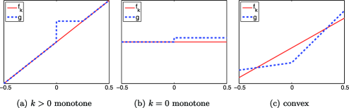
Figure 1: Plots of $f_{k}$ and a least favorable function $g$ in Example 1 with the constraints $|g(0)-f_{k}(0)|=a$.

Example 2.

As a second example which is also both monotonically nondecreasing and convex consider the function $f(t)=k_{1}t+k_{2}t^{r}I\ (0<t\leq\frac{1}{2})$ where $r\geq 1$ and $k_{1}\geq 0$ and $k_{2}>0$ are constants.

We consider the cases $r=1$ and $r>1$ separately. When $r=1$ the function is piecewise linear with the change of slope at $0$. In this case suppose $0<a\leq\frac{k_{1}+k_{2}}{2}$. A monotonically nondecreasing function $g\in F_{m}$ that minimize $\|g-f\|_{2}$ subject to the constraint that $|g(0)-f(0)|=a$ is given by $g(t)=f(t)$ if $t<0$, $g(t)=a$ if $0\leq t\leq b$, and $g(t)=f(t)$ if $t>b$, where $b$ satisfies $f(b)=a$. The constraint $a\leq\frac{k_{1}+k_{2}}{2}$ is to guarantee that such a $b$ exists with $b\leq\frac{1}{2}$. Then we have $\|g-f\|_{2}=a^{{3}/{2}}(3(k_{1}+k_{2}))^{-{1}/{2}}$, and it follows that if $\varepsilon^{2}\leq\frac{1}{24}(k_{1}+k_{2})^{2}$,

$$\omega(\varepsilon,f,F_{m})=\bigl{(}3(k_{1}+k_{2})\bigr{)}^{{1}/{3}}\varepsilon^{{2}/{3}}$$

and consequently for $n\geq\frac{24z_{\alpha}^{2}}{(k_{1}+k_{2})^{2}}$,

$$L^{*}_{\alpha}(f,F_{m})\geq\biggl{(}1-\frac{1}{\sqrt{2\pi}z_{\alpha}}\biggr{)}\bigl{(}3(k_{1}+k_{2})\bigr{)}^{{1}/{3}}z^{2/3}_{\alpha}n^{-{1/3}}.$$

We can also give a lower bound on the expected length for this same function for confidence intervals which guarantee coverage over the class of convex functions. Suppose $0<a\leq\frac{k_{2}}{4}$. Here we need to find the convex $h$ that minimizes $\|h-f\|_{2}$ subject to the constraints that $|h(0)-f(0)|=a$. It is given by $h(t)=f(t)$ if $t\leq-\frac{2a}{k_{2}}$, $h(t)=(\frac{k_{2}}{2}+k_{1})t+a$ if $-\frac{2a}{k_{2}}\leq t\leq\frac{2a}{k_{2}}$ and $h(t)=f(t)$ if $t\geq\frac{2a}{k_{2}}$. Then $\|f-g\|_{2}=2a^{{3}/{2}}/(3k_{2})^{{1}/{2}}$ and it follows that if $\varepsilon^{2}\leq\frac{k_{2}^{2}}{48}$,

$$\omega(\varepsilon,f,F_{c})=(3k_{2}/4)^{{1}/{3}}\varepsilon^{{2}/{3}}.$$

Hence, for $n\geq\frac{48z_{\alpha}^{2}}{k_{2}^{2}}$,

$$L^{*}_{\alpha}(f,F_{c})\geq\biggl{(}1-\frac{1}{\sqrt{2\pi}z_{\alpha}}\biggr{)}(3k_{2}/4)^{{1}/{3}}z^{2/3}_{\alpha}n^{-{1/3}}.$$

We now turn to the case where $r>1$. Suppose $0<a\leq\frac{k_{1}}{2}+k_{2}(\frac{1}{2})^{r}$. In this case the monotonically nondecreasing function $g$ that minimizes $\|g-f\|_{2}$ subject to the constraints that $|g(0)-f(0)|=a$ is given by $g(t)=f(t)$ if $t<0$, $g(t)=a$ if $0\leq t\leq b$ and $g(t)=f(t)$ if $t>b$, where $b$ satisfies $f(b)=a$. As before the condition $0<a\leq\frac{k_{1}}{2}+k_{2}(\frac{1}{2})^{r}$ guarantees that $b$ exists with $b<\frac{1}{2}$. In this case $a^{{3}/{2}}(3k_{1})^{-{1}/{2}}-ca^{s}\leq\|g-f\|_{2}\leq a^{{3}/{2}}(3k_{1})^{-{1}/{2}}+ca^{s}$ for some constant $c>0$ and $s>3/2$. It follows that if $\varepsilon^{2}\leq\frac{1}{24}k_{1}^{2}+(1+\frac{1}{2r+1}-\frac{2}{r+1})(\frac{1}{2})^{2r+1}k_{2}^{2}+(\frac{1}{2}-\frac{1}{r+1}+\frac{1}{r+2})(\frac{1}{2})^{r+1}k_{1}k_{2}$, then

$$\omega(\varepsilon,f,F_{m})=(3k_{1})^{{1}/{3}}\varepsilon^{{2}/{3}}\bigl{(}1+o(1)\bigr{)}.$$

Hence,

$$L^{*}_{\alpha}(f,F_{m})\geq\biggl{(}1-\frac{1}{\sqrt{2\pi}z_{\alpha}}\biggr{)}(3k_{1})^{{1}/{3}}z^{2/3}_{\alpha}n^{-{1/3}}\bigl{(}1+o(1)\bigr{)}.$$

For a bound on the expected length of this same function for confidence intervals with coverage guaranteed over the collection of convex functions, we suppose $0<a\leq k_{2}(\frac{1}{2})^{r+1}$. In this case the convex function $h$ that minimizes $\|h-f\|_{2}$ subject to the constraints that $|h(0)-f(0)|=a$, is given by $h(t)=kt+a$, $k>k_{1}$, if $x_{0}\leq t\leq x_{1}$ and $h(t)=f(t)$ otherwise, where $(x_{0},cx_{0})$ and $(x_{1},cx_{1}+x_{1}^{r})$ are the intersection points of $f(t)$ and the line $kt+a$. Then the function $h$ with slope $k_{0}$ that minimize $\|h-f\|_{2}$ would be the least favorable function. It follows that, if $\varepsilon^{2}\leq\frac{k_{2}^{2}}{24}(\frac{1}{2})^{2r}$,

$$\omega(\varepsilon,f,F_{c})=C(r)k_{2}^{{1}/{(2r+1)}}\varepsilon^{{2r}/{(2r+1)}}$$

and consequently for $n\geq\frac{24z_{\alpha}^{2}2^{2r}}{k_{2}^{2}}$,

$$L^{*}_{\alpha}(f,{\mathcal{F}}_{c})\geq\biggl{(}1-\frac{1}{\sqrt{2\pi}z_{\alpha}}\biggr{)}C(r)k_{2}^{{1}/{(2r+1)}}z_{\alpha}^{{2r}/{(2r+1)}}n^{-{r/(2r+1)}},$$

where $C(r)>0$ is a constant depending on $r$ only.

It is interesting to note that in this example the rates of convergence for $L^{*}_{\alpha}(f,{\mathcal{F}}_{m})$ and $L^{*}_{\alpha}(f,{\mathcal{F}}_{c})$ are the same for the case $r=1$, and are different when $r>1$. Plots illustrating shapes of functions $f$ and a least favorable function $g$ are shown as below in Figure 2.

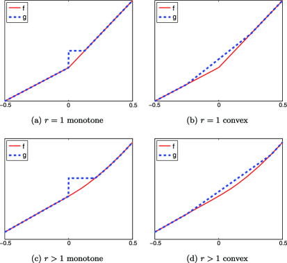
Figure 2: Plots of $f$ and a least favorable function $g$ in Example 2 with the constraints $|g(0)-f(0)|=a$.

Next we consider a function which is monotonically nondecreasing but not convex.

Example 3.

Let $f(t)=kt^{r}$ for some constant $k>0$ and $r=2l+1$ or $r=\frac{1}{2l+1}$ for $l=0,1,2,\ldots.$ Suppose that $a<(\frac{1}{2})^{r}k$. In this case a function $g$ that minimizes $\|g-f\|_{2}$ subject to the constraint that $|g(0)-f(0)|=a$ is given by $g(t)=f(t)$ if $t<0$, $g(t)=a$ if $0\leq t\leq b$ and $g(t)=f(t)$ if $t>b$, where $b$ satisfies $f(b)=a$. As before the condition $a<(\frac{1}{2})^{r}k$ guarantees that $b$ exists with $b<\frac{1}{2}$. Then $\|g-f\|_{2}=a^{1+({1}/{(2r)})}/k^{{1}/{(2r)}}(2r^{2}/(r+1)(2r+1))^{{1}/{2}}$, and it follows that when $\varepsilon^{2}\leq(\frac{1}{2})^{2r+1}k^{2}\frac{2r^{2}}{(r+1)(2r+1)}$,

$$\omega(\varepsilon,f,F_{m})=\biggl{(}\frac{(r+1)(2r+1)k}{2r^{2}}\biggr{)}^{{r}/{(2r+1)}}\varepsilon^{{2r}/{(2r+1)}}.$$

Hence for $n\geq\frac{2^{2r+1}(r+1)(2r+1)z_{\alpha}^{2}}{2r^{2}k^{2}}$,

$$L^{*}_{\alpha}(f,{\mathcal{F}}_{c})\geq\biggl{(}1-\frac{1}{\sqrt{2\pi}z_{\alpha}}\biggr{)}\biggl{(}\frac{(r+1)(2r+1)k}{2r^{2}}\biggr{)}^{{r}/({2r+1)}}z_{\alpha}^{2r/(2r+1)}n^{-{r/(2r+1)}},$$

and once again it is clear that the rate at which the expected length decreases to zero depends strongly on the value of $r$.

As a final example we consider a function which is convex but not monotonically nondecreasing.

Example 4.

Let $f(t)=t^{2}$. Suppose that $a<1/2$. In this case the function $g$ that minimizes $\|g-f\|_{2}$ subject to the constraint that $|g(0)-f(0)|=a$ is given by $g(t)=-3\sqrt{a/2}t-a$ if $-\sqrt{2a}\leq t\leq 0$, $g(t)=3\sqrt{a/2}t-a$ if $0\leq t\leq\sqrt{2a}$ and $g(t)=f(t)$ otherwise. Then $\|g-f\|_{2}=2^{5/4}/\sqrt{15}a^{5/4}$ and it follows that when $\varepsilon^{2}\leq 1/\sqrt{15}$,

$$\omega(\varepsilon,f,F_{m})=\frac{15^{2/5}}{2}\varepsilon^{{4}/{5}}.$$

Hence for $n\geq\sqrt{15}z_{\alpha}^{2}$,

$$L^{*}_{\alpha}(f,{\mathcal{F}}_{c})\geq\biggl{(}1-\frac{1}{\sqrt{2\pi}z_{\alpha}}\biggr{)}\frac{15^{2/5}}{2}z_{\alpha}^{{4}/{5}}n^{-{2}/{5}}.$$

A similar minimization problem is solved in Dümbgen (2003).

Plots illustrating shapes of functions $f$ and a least favorable function $g$ for both Examples 3 and 4 are shown in Figure 3.

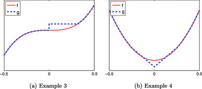
Figure 3: Plots of $f$ and a least favorable function $g$ in Examples 3 and 4 with the constraints $|g(0)-f(0)|=a$.

3 Confidence procedures

In this section we both construct and give an analysis of adaptive confidence intervals for monotone functions and convex functions. The procedures are easily implementable. We consider the class of monotonically nondecreasing functions and the class of convex functions. Concave functions and monotonically nonincreasing functions can be handled similarly.

3.1 Construction

The construction is split into two steps. In the first step a countable collection of confidence intervals is created each of which has guaranteed coverage probability. These intervals are based on a collection of pairs of linear estimators. For each interval one of the estimators has nonnegative bias and the other nonpositive bias. The one-sided control of the bias of these estimators is a key special feature in these problems and an important part of what makes it possible to adapt to every individual function. Moreover for each function $f$ this collection has at least one interval with expected length within a constant factor of the local modulus bound given in Theorem 1. The second step is to select from this collection a particular interval.

In the case of monotonically nondecreasing functions we take for each $j\geq 2$, pairs of estimators $\delta_{j}^{R}=2^{j}(Y(2^{-j})-Y(0))$ and $\delta_{j}^{L}=2^{j}(Y(0)-Y(-2^{-j}))$. Then for estimating $f(0)$ it is easy to check that $\delta_{j}^{R}$ has nonnegative and monotonically nonincreasing biases while $\delta_{j}^{L}$ have nonpositive and monotonically nondecreasing biases. The one-sided control of the biases of these estimators over the class of all monotonically nondecreasing functions easily allows for the construction of a confidence interval. For that we shall need the standard deviation of $\delta_{j}^{R}$ and $\delta_{j}^{L}$. In order to give a unified treatment in both the monotone and convex case it is useful to establish a common notation. Here we shall set $\sigma^{2}_{j}=\frac{2^{j-1}}{n}$. It is then easy to check that both $\delta_{j}^{R}$ and $\delta_{j}^{L}$ have a standard deviation of $\sqrt{2}\sigma_{j}$. It is then also easy to see that for each $j\geq 2$, the confidence interval $\mathrm{CI}^{m}_{j}(\alpha)$ given by

$$\mathrm{CI}^{m}_{j}(\alpha)=\bigl{[}\delta_{j}^{L}-z_{\alpha/2}\sqrt{2}\sigma_{j},\delta_{j}^{R}+z_{\alpha/2}\sqrt{2}\sigma_{j}\bigr{]}$$ (7)

has guaranteed coverage of $1-\alpha$. We should, however, note that in (7) the left endpoint of the interval may be larger than the right endpoint in which case we adopt the convention that the confidence interval is just the empty set. The length of this confidence interval is then $\max(\delta_{j}^{R}-\delta_{j}^{L}+2\sqrt{2}z_{\alpha/2}\sigma_{j},0)$.

In the case of convex functions for $j\geq 1$, let $\delta_{j}=2^{j-1}(Y(2^{-j})-Y(-2^{-j}))$ and let $\tilde{\delta}_{j}=2\delta_{j+1}-\delta_{j}$.

The following lemma shows that for convex functions $\delta_{j}$ have nonnegative and monotonically nonincreasing biases and that $\tilde{\delta}_{j}$ have nonpositive and monotonically nondecreasing biases.

Lemma 1

For any convex function $f$,

$$0 \leq \operatorname{Bias}(\delta_{j+1})\leq\tfrac{1}{2}\operatorname{Bias}(\delta_{j}),$$ (8)

$$E\delta_{j}-3E\delta_{j+1}+2E\delta_{j+2} \geq 0.$$ (9)

It is also easy to check that the standard deviation of $\delta_{j}$ is equal to $\sigma_{j}$ where $\sigma^{2}_{j}=\frac{2^{j-1}}{n}$ and that $2\delta_{j+1}-\delta_{j}$ has a standard deviation of ${\sqrt{5}}\sigma_{j}$. It then follows from the signs of the biases of $\delta_{j+1}$ and $2\delta_{j+1}-\delta_{j}$ that for any given $j$,

$$\mathrm{CI}_{j}^{c}(\alpha)=[2\delta_{j+1}-\delta_{j}-z_{\alpha/2}{\sqrt{5}}\sigma_{j},\delta_{j+1}+z_{\alpha/2}\sigma_{j+1}]$$ (10)

gives a confidence interval with coverage probability of at least $1-\alpha$. We should also note once again that the left endpoint of the interval may be larger than the right endpoint in which case the confidence interval is taken to be the empty set, and so in this case the length of this confidence interval is $\max(\delta_{j}-\delta_{j+1}+(\sqrt{5}+\sqrt{2})z_{\alpha/2}\sigma_{j},0)$.

These results, for which a more formal proof is given in Section 6 are summarized in the following proposition.

Proposition 1

For every $j\geq 2$, the confidence interval $\mathrm{CI}_{j}^{m}$ defined in (7) has coverage probability of at least $1-{\alpha}$ for all monotonically nondecreasing functions $f\in F_{m}$, and for every $j\geq 1$, the confidence interval $\mathrm{CI}_{j}^{c}$ defined in (10) has coverage probability of at least $1-{\alpha}$ for all convex functions $f\in F_{c}$.

The second stage in the construction is that of selecting from these collections of intervals the one to be used. First note that one should not select the shortest interval since the collections defined in (7) and (10) will always contain one which corresponds to the empty set. A more sensible goal is to try to select the interval with the smallest expected length or at least one which has expected length close to the smallest expected length.

The approach we take here is to choose an interval for which the expected length is of the same order of magnitude as the standard deviation of the length. Such an interval will always have expected length close to the shortest expected length. For the case of monotonically nondecreasing functions the selection of the interval from the countable collection in (7) can be done by creating another collection of estimators which can be used to estimate the expected length of the intervals.

More specifically set $\xi_{j}=2^{j-1}(Y(2^{-j+1})-Y(2^{-j}))-2^{j-1}(Y(-2^{-j})-Y(-2^{-j+1}))$. Then for $j\geq 2$, $\xi_{j}$’s are independent of each other and both $\delta_{j}^{R}$ and $\delta_{j}^{L}$ are independent of $\xi_{k}$ for every $k\leq j$. We should note that the estimators $\xi_{j}$ are similar to $\delta_{j}^{R}-\delta_{j}^{L}$ in that they are both differences of averages of $Y$ to the left and right of the origin and thus estimate the average local change of the function. However $\delta_{j}^{R}-\delta_{j}^{L}$ are not independent for different $j$ whereas the $\xi_{j}$ are independent. It is thus natural to view the $\xi_{j}$ as a surrogate for $\delta_{j}^{R}-\delta_{j}^{L}$ with the technical advantage that they are independent. The selection of a $j$ for which $\xi_{j}$ has expected value close to $\sigma_{j}$ will then result in a confidence interval $\mathrm{CI}_{j}^{m}$ close to the one with the smallest expected length. The independence properties of the $\xi_{j}$ allows us to guarantee a $1-\alpha$ coverage probability while making this selection.

More specifically the construction proceeds as follows. Let

$$\hat{j}=\inf_{j}\biggl{\{}j\dvtx\xi_{j}\leq\frac{3}{2}z_{\alpha}\sigma_{j}\biggr{\}}$$ (11)

and define the final confidence interval by

$$\mathrm{CI}^{m}_{*}=\mathrm{CI}_{\hat{j}}^{m}(\alpha).$$ (12)

Before we turn to the analysis of this procedure we also introduce here a related confidence procedure in the convex case. Here rather than introducing an independent estimate of the difference between the two estimators used in constructing the confidence interval, we proceed more directly. The basic idea is similar, but the dependence between the estimates of $j$ and the confidence interval constructed from this estimate requires that we adjust the original coverage level of our $\mathrm{CI}_{j}^{c}$.

More specifically let $T_{j}=\delta_{j}-\delta_{j+1}$. When the expected value of $T_{j}$ is the same order as $\sigma_{j}$, the confidence interval $\mathrm{CI}_{j}^{c}$ will then be close to the one with the smallest expected length. Our estimate of $j$ is given by an empirical version, namely

$$\hat{j}=\inf_{j}\{j\dvtx T_{j}\leq z_{\alpha}\sigma_{j}\}.$$ (13)

Although this estimate can be used to select the appropriate $\mathrm{CI}_{j}^{c}$ to use, as just mentioned, care also needs to be taken to make sure that the resulting selected interval maintains the required coverage probability. The analysis given below shows that a choice of $\alpha/6$ in the construction of the original collection of intervals guarantees an overall coverage probability of $\alpha$. Thus in the case of convex functions, we define our interval by

$$\mathrm{CI}^{c}_{*}=\mathrm{CI}_{\hat{j}}^{c}\biggl{(}\frac{\alpha}{6}\biggr{)}.$$ (14)

3.2 Analysis of the confidence intervals

In this section we present the properties of the confidence intervals $\mathrm{CI}_{*}^{m}$ and $\mathrm{CI}_{*}^{c}$ defined by (12) and (14) focusing on the coverage and the expected length of these intervals.

We begin with the confidence interval $\mathrm{CI}_{*}^{m}$. In this case it is easy to check the coverage probability of $\mathrm{CI}_{*}^{m}$ by the independence of the interval $\mathrm{CI}_{j}^{m}$ and $\xi_{k}$ for every $k$ satisfying $2\leq k\leq j$.

The key to the analysis of the expected length is the introduction of $j_{*}^{m}$ where

$$j_{*}^{m}=\mathop{\arg\min}_{j}\{j\dvtx E\xi_{j}\leq z_{\alpha}\sigma_{j}\}.$$ (15)

The analysis of the expected length relies on showing that $\hat{j}$ is highly concentrated around $j_{*}^{m}$. The concentration of $\hat{j}$ around $j_{*}^{m}$ then provides a bound on the expected length of $\mathrm{CI}^{*}$. These results, for which a proof is given in Section 6 are summarized in the following theorem.

Theorem 2

Let $0<\alpha\leq 0.2$. The confidence interval $\mathrm{CI}_{*}^{m}$ defined in (12) has coverage probability of at least $1-\alpha$ for all monotonically nondecreasing functions $f\in F_{m}$ and satisfies

$$E_{f}L\bigl{(}\mathrm{CI}_{*}^{m}\bigr{)}\leq 1.21(3z_{\alpha}+2\sqrt{2}z_{{\alpha}/{2}})\sigma_{j_{*}^{m}}\leq c_{0}z_{\alpha}\sigma_{j_{*}^{m}},$$ (16)

where $c_{0}$ is a constant and can be taken to be $8.85$ for all $0<\alpha\leq 0.2$.

Remark 1.

The constant $c_{0}$ in Theorem 2 depends on the upper limit of $\alpha$. $c_{0}$ can be smaller if the upper limit on $\alpha$ is reduced. For example, for common choices of $\alpha=0.05$ or 0.01, $c_{0}\leq 7.71$ for $\alpha=0.05$, and $c_{0}\leq 7.42$ for $\alpha=0.01$.

Theorem 2 shows that the coverage probability is attained and also provides an upper bound on the expected length in terms of $\sigma_{j_{*}^{m}}$. In order to establish that this expected length is within a constant factor of the lower bound given in Theorem 1, we need to provide a lower bound for $L_{\alpha}^{*}(f,F_{m})$ in terms of $z_{\alpha}\sigma_{j_{*}^{m}}$. This connection is given in the following theorem.

Theorem 3

Let $0<\alpha\leq 0.2$ and let $f\in F_{m}$. Then

$$L_{\alpha}^{*}(f,F_{m})\geq\biggl{(}1-\frac{1}{\sqrt{2\pi}z_{\alpha}}\biggr{)}\frac{1}{\sqrt{2}}z_{\alpha}\sigma_{j_{*}^{m}}.$$ (17)

Combining Theorems 2 and 3, we have

$$E_{f}L\bigl{(}\mathrm{CI}_{*}^{m}\bigr{)}\leq c_{1}L_{\alpha}^{*}(f,F_{m})$$ (18)

for all monotonically nondecreasing functions $f\in F_{m}$, where $c_{1}$ is a constant depending on $\alpha$ only. For example, $c_{1}$ can be taken to be $14.40$ for $\alpha=0.05$ and $12.67$ for $\alpha=0.01$. Hence, the confidence interval $\mathrm{CI}_{*}^{m}$ is uniformly within a constant factor of the benchmark $L_{\alpha}^{*}(f,F_{m})$ for all monotonically nondecreasing functions $f$ and all confidence level $1-\alpha\geq 0.8$.

We now turn to an analysis of the properties of the confidence interval $\mathrm{CI}_{*}^{c}$ defined in (14). The key to this analysis is the introduction of $j_{*}^{c}$ where

$$j_{*}^{c}=\mathop{\arg\min}_{j}\biggl{\{}j\dvtx ET_{j}\leq\frac{2}{3}z_{\alpha}\sigma_{j}\biggr{\}}.$$ (19)

The analysis of both the coverage probability and the expected length relies on showing that $\hat{j}$ is highly concentrated around $j_{*}^{c}$. The probability of not covering $f(0)$ can be bounded by

$$P\bigl{(}f(0)\notin\mathrm{CI}_{*}^{c}\bigr{)} \leq P\bigl{(}\hat{j}\leq j_{*}^{c}-3\bigr{)}+P\bigl{(}\hat{j}\geq j_{*}^{c}+3\bigr{)}$$

$${}+\sum_{l=-2}^{2}P\bigl{(}f(0)\notin\mathrm{CI}_{j_{*}^{c}+l}\bigr{)}.$$

The first two terms are controlled by the high concentration of $\hat{j}$ around $j_{*}^{c}$, and the last term is controlled by Proposition 1 which bounds the coverage probability of any given $j$. The concentration of $\hat{j}$ around $j_{*}^{c}$ also allows control on the expected length of $\mathrm{CI}_{*}^{c}$ which leads to the following theorem.

Theorem 4

Let $0<\alpha\leq 0.2$. The confidence interval $\mathrm{CI}_{*}^{c}$ defined in (14) has coverage probability of at least $1-\alpha$ for all convex $f$ and satisfies

$$E_{f}L\bigl{(}\mathrm{CI}_{*}^{c}\bigr{)}\leq 1.25\bigl{(}z_{\alpha}+(\sqrt{5}+\sqrt{2})z_{\alpha/12}\bigr{)}\sigma_{j_{*}^{c}}\leq c_{0}z_{\alpha}\sigma_{j_{*}^{c}},$$ (21)

where $c_{0}$ is a constant and can be taken to be $12.79$ for all $0<\alpha\leq 0.2$.

Remark 2.

The constant $c_{0}$ in Theorem 4 depends on the upper limit of $\alpha$. $c_{0}$ can be smaller if the upper limit on $\alpha$ is reduced. For example, for common choices of $\alpha=0.05$ or 0.01, $c_{0}\leq 8.57$ for $\alpha=0.05$, and $c_{0}\leq 7.42$ for $\alpha=0.01$.

Theorem 4 shows that the coverage probability is attained and also provides an upper bound on the expected length in terms of $\sigma_{j_{*}^{c}}$. As was the case for monotone functions, in order to to establish that this expected length for convex functions is within a constant factor of the lower bound given in Theorem 1, we need to provide a lower bound for $L_{\alpha}^{*}(f,F_{c})$ in terms of $z_{\alpha}\sigma_{j_{*}^{c}}$. This connection is given in the following theorem.

Theorem 5

Let $0<\alpha\leq 0.2$ and let $f\in F_{c}$. Then

$$L_{\alpha}^{*}(f,F_{c})\geq\biggl{(}1-\frac{1}{\sqrt{2\pi}z_{\alpha}}\biggr{)}\frac{\sqrt{2}}{3}z_{\alpha}\sigma_{j_{*}^{c}}.$$ (22)

Theorems 4 and 5 together yield

$$E_{f}L\bigl{(}\mathrm{CI}_{*}^{c}\bigr{)}\leq c_{2}L_{\alpha}^{*}(f,F_{c})$$ (23)

for all convex functions $f\in F_{c}$, where $c_{2}$ is a constant depending on $\alpha$ only. For example, $c_{2}$ can be taken to be $24$ for $\alpha=0.05$ and $19$ for $\alpha=0.01$. Hence, the confidence interval $\mathrm{CI}_{*}^{c}$ is uniformly within a constant factor of the benchmark $L_{\alpha}^{*}(f,F_{c})$ for all convex functions $f$ and all confidence levels $1-\alpha\geq 0.8$.

4 Nonparametric regression

We have so far focused on the white noise model. The theory presented in the earlier sections can also easily be extended to nonparametric regression. Consider the regression model

$$y_{i}=f(x_{i})+\sigma z_{i},\qquad i=-n,-(n-1),-1,0,1,\ldots,n,$$ (24)

where $x_{i}={i\over 2n}$ and $z_{i}\stackrel{{\scriptstyle\mathrm{i.i.d.}}}{{\sim}}N(0,1)$ and where for notational convenience we index the observations from $-n$ to $n$. Note that the noise level $\sigma$ can be accurately estimated easily, as in Hall, Kay and Titterington (1990) or Munk et al. (2005). See also Wang et al. (2008). We shall thus assume it is known in this section. Then under the assumption that $f$ is convex or monotone, we wish to provide a confidence interval for $f(0)$.

4.1 Monotone regression

Let $J=\lfloor\log_{2}n\rfloor$. For $1\leq j\leq J$ define the local average estimators

$$\bar{\delta}_{j}^{R}=2^{-j+1}\sum_{k=1}^{2^{j-1}}y_{k}\quad\mbox{and}\quad\bar{\delta}_{j}^{L}=2^{-j+1}\sum_{k=1}^{2^{j-1}}y_{-k}.$$ (25)

We should note that the indexing scheme is the reverse of that given for the white noise with drift process. Here estimators $\bar{\delta}_{j}^{R}$ (or $\bar{\delta}_{j}^{L}$) with small values of $j$ have smaller bias (or larger bias) and larger variance than those with larger values of $j$.

As in the white noise model it is easy to check that $\bar{\delta}_{j}^{R}$ has nonnegative bias and $\bar{\delta}_{j}^{L}$ has nonpositive bias. Simple calculations show that the variance of $\bar{\delta}_{j}^{R}$ and $\bar{\delta}_{j}^{L}$ are both $2\sigma_{j}^{2}$, where $\sigma_{j}^{2}=2^{-j}\sigma^{2}$. It is also important to introduce $\bar{\xi}_{j}$ as in the white noise case, where $\bar{\xi}_{j}=2^{-j}\sum_{k=2^{j-1}+1}^{2^{j}}(y_{k}-y_{-k})$. It is easy to check that $E\bar{\xi}_{j}\leq E\bar{\xi}_{j+1}$, $\bar{\xi}_{j}$’s are independent with each other, and both $\bar{\delta}_{j}^{R}$ and $\bar{\delta}_{j}^{L}$ are independent with $\bar{\xi}_{k}$ for every $k\geq j$.

It then follows that $\mathrm{CI}_{j}^{m}=[\bar{\delta}_{j}^{L}-z_{{\alpha}/{2}}\sqrt{2}\sigma_{j},\bar{\delta}_{j}^{R}+z_{{\alpha}/{2}}\sqrt{2}\sigma_{j}]$ has guaranteed coverage probability of at least $1-\alpha$ over all monotonically nondecreasing functions.

Now set

$$\hat{j}=\cases{\displaystyle\max_{j}\biggl{\{}j\dvtx\bar{\xi}_{j}\leq\frac{3}{2}z_{\alpha}\sigma_{j}\biggr{\}},&\quad$\mbox{if $\displaystyle\bar{\xi}_{1}\leq\frac{3}{2}z_{\alpha}\sigma_{1}$;}$\vspace*{2pt}\cr 1,&\quad$\mbox{otherwise,}$}$$ (26)

and define the confidence interval to be

$$\mathrm{CI}_{*}^{m}=\mathrm{CI}_{\hat{j}}^{m}.$$ (27)

The properties of this confidence interval can then be analyzed in the same way as before and can be shown to be similar to those for the white noise model. In particular, the following result holds.

Theorem 6

Let $0<\alpha\leq 0.2$. The confidence interval $\mathrm{CI}_{*}^{m}$ defined in (27) has coverage probability of at least $1-\alpha$ for all monotone functions $f$ and satisfies

$$E_{f}L\bigl{(}\mathrm{CI}_{*}^{m}\bigr{)}\leq C_{1}L_{\alpha}^{*}(f,F_{m})$$ (28)

for all monotonically nondecreasing functions $f\in F_{m}$, where $C_{1}>0$ is a constant depending on $\alpha$ only.

4.2 Convex regression

As in the monotone case, set $J=\lfloor\log_{2}n\rfloor$. For $1\leq j\leq J$ define the local average estimators

$$\bar{\delta}_{j}=2^{-j}\sum_{k=1}^{2^{j-1}}(y_{-k}+y_{k}).$$ (29)

We should note that this indexing scheme is the reverse of that given for the white noise with drift process. Here estimators $\bar{\delta}_{j}$ with small values of $j$ have smaller bias and larger variance than those with larger values of $j$.

As in the white noise model it is easy to check that $\bar{\delta}_{j}$ has nonnegative bias. It is also important to introduce an estimate which has a similar variance but is guaranteed to have nonpositive bias. The key step is to introduce

$$T_{j}=\bar{\delta}_{j}-\bar{\delta}_{j-1}$$ (30)

as an estimate of the bias of $\bar{\delta}_{j}$. The following lemma gives the required properties of $\bar{\delta}_{j}$ and $T_{j}$.

Lemma 2

For any convex function $f$,

$$2ET_{j} \leq ET_{j+1},$$ (31)

$$0 \leq \operatorname{Bias}(\bar{\delta}_{j})\leq{2^{j-1}+1\over 2^{j}+1}\operatorname{Bias}(\bar{\delta}_{j+1}).$$ (32)

From (32) it is clear that the biases of the estimators $\bar{\delta}_{j}$ are nonnegative and monotonically nondecreasing. In addition straightforward calculations using both (31) and (32) show that the estimators

$$\delta^{L}_{j}=\bigl{(}2+2^{-(j-1)}\bigr{)}\bar{\delta}_{j}-\bigl{(}1+2^{-(j-1)}\bigr{)}\bar{\delta}_{j+1}=\bar{\delta}_{j}-\bigl{(}1+2^{-(j-1)}\bigr{)}T_{j+1}$$

have a nonpositive and monotonically nonincreasing biases. Simple calculations show that the variance of $\delta^{L}_{j}$ is $\tau_{j}^{2}=(5+2^{-j+3}+2^{-2j+2})2^{-j-1}\sigma^{2}$.

It then follows that $\mathrm{CI}_{j}^{c}=[\bar{\delta}_{j}-(1+2^{-(j-1)})T_{j+1}-z_{\alpha/12}\tau_{j},\bar{\delta}_{j}+z_{\alpha/12}\sigma_{j}]$ has coverage over all convex functions.

Now set

$$\hat{j}=\cases{\displaystyle\max_{j}\{j\dvtx T_{j}\leq z_{\alpha}\sigma_{j}\},&\quad$\mbox{if $T_{2}\leq z_{\alpha}\sigma_{2}$;}$\vspace*{2pt}\cr 1,&\quad$\mbox{otherwise,}$}$$ (33)

and define the confidence interval to be

$$\mathrm{CI}_{*}^{c}=\mathrm{CI}_{\hat{j}}^{c}.$$ (34)

This confidence interval shares similar properties as the one for the white noise model. In particular, the following result holds.

Theorem 7

Let $0<\alpha\leq 0.2$. The confidence interval $\mathrm{CI}_{*}^{c}$ defined in (34) has coverage probability of at least $1-\alpha$ for all convex function $f$ and satisfies

$$E_{f}L\bigl{(}\mathrm{CI}_{*}^{c}\bigr{)}\leq C_{2}L_{\alpha}^{*}(f,F_{c})$$ (35)

for all convex function $f\in F_{c}$, where $C_{2}>0$ is a constant depending on $\alpha$ only.

5 Discussion

The major emphasis of the paper has been to show that with shape constraints it is possible to construct confidence intervals that have expected length that adapts to individual functions. In this section we shall discuss briefly the maximum expected lengths of our procedures over Lipschitz classes that are either monotone or convex in a way that is similar to that provided in Dümbgen (1998, 2003) for the maximum width of a confidence band. We shall also explain how our results can be extended to the problem of estimating the value of $f$ at points other than $0$.

5.1 Minimax results

Although the focus of the present paper has been on the construction of a confidence interval with the expected length adaptive to each individual convex or monotone function, these results do yield immediately adaptive minimax results for the expected length in the conventional sense. Define

$$F_{c}(\beta,M)=F_{c}\cap\Lambda(\beta,M)\quad\mbox{and}\quad F_{m}(\beta,M)=F_{m}\cap\Lambda(\beta,M).$$

The following results are direct consequence of Theorems 2 and 4.

Corollary 1

(i) The confidence interval $\mathrm{CI}_{*}^{m}$ defined in (12) satisfies

$$\sup_{f\in F_{m}(\beta,M)}E_{f}L\bigl{(}\mathrm{CI}_{*}^{m}\bigr{)}\leq C_{1}M^{1/(1+2\beta)}n^{-{\beta/(1+2\beta)}}$$ (36)

simultaneously for all $0\leq\beta\leq 1$ and $1<M<\infty$, for some absolute constant $C_{1}>0$.

(ii) The confidence interval $\mathrm{CI}_{*}^{c}$ defined in (14) satisfies

$$\sup_{f\in F_{c}(\beta,M)}E_{f}L\bigl{(}\mathrm{CI}_{*}^{c}\bigr{)}\leq C_{2}M^{1/(1+2\beta)}n^{-{\beta/(1+2\beta)}}$$ (37)

simultaneously for all $1\leq\beta\leq 2$ and $1<M<\infty$, for some absolute constant $C_{2}>0$.

We should note that these ranges of Lipschitz classes are the only ones of interest in these cases. In particular suppose that $\mathrm{CI}$ is a confidence interval with guaranteed coverage over the class of monotonically nondecreasing functions. Then for any $\beta>1$ the class $\Lambda(\beta,M)$ includes the linear function $f_{k}(t)=kt$. As shown in Example 1 in Section 2.2,

$$L^{*}_{\alpha}(f_{k},F_{m})\geq\biggl{(}1-\frac{1}{\sqrt{2\pi}z_{\alpha}}\biggr{)}(3k)^{{1}/{3}}z^{2/3}_{\alpha}n^{-{1/3}}.$$

Hence,

$$\sup_{f\in F_{m}(\beta,M)}E_{f}L(\mathrm{CI}) \geq \sup_{k}L^{*}_{\alpha}(f_{k},F_{m})$$

$$= \sup_{k}\biggl{(}1-\frac{1}{\sqrt{2\pi}z_{\alpha}}\biggr{)}(3k)^{{1}/{3}}z^{2/3}_{\alpha}n^{-{1/3}}=\infty.$$

A similar results holds for convex functions assumed to belong to $\Lambda(\beta,M)$ with $\beta>2$. On the other hand suppose $f$ is convex and assumed to belong to $\Lambda(\beta,M)$ with $\beta<1$. Then from the assumption that $f$ is in $\Lambda(\beta,M)$ it follows that $|f(1/2)-f(-1/2)|\leq M$. Convexity then shows that $f\in\Lambda(1,M)$ and the maximum expected length over this class is given above.

5.2 Confidence interval at other points

The focus of the present paper has been on the problem of estimating the value of $f(0)$. The basic development is similar for any other point $t$ in the interior of the interval $[-1/2,1/2]$ unless $t$ is near to the boundary. More specifically for any $0\leq t<1/2$ we can consider estimators $\delta_{j}^{R}(t)=2^{j}(Y(t+2^{-j})-Y(t))$ and $\delta_{j}^{L}(t)=2^{j}(Y(t)-Y(t-2^{-j}))$ where $j\geq-\log_{2}(\frac{1}{4}-\frac{t}{2})$ for monotone functions and $\delta_{j}(t)=2^{j-1}(Y(t+2^{-j})-Y(t-2^{-j}))$ where $j\geq-\log_{2}(\frac{1}{2}-t)$ for convex functions. The basic theory is the same as before.

For monotonically nondecreasing functions, the confidence interval $\mathrm{CI}_{j}^{m}$ is replaced by

$$\mathrm{CI}_{j}^{m}(t)=\bigl{[}\delta_{j}^{L}(t)-z_{{\alpha}/{2}}\sqrt{2}\sigma_{j},\delta_{j}^{R}(t)+z_{{\alpha}/{2}}\sqrt{2}\sigma_{j}\bigr{]}$$

and the choice of $\hat{j}$ is given by

$$\hat{j}(t)=\inf_{j\geq-\log_{2}({1}/{4}-({t}/{2}))}\biggl{\{}j\dvtx\xi_{j}(t)\leq\frac{3}{2}z_{\alpha}\sigma_{j}\biggr{\}},$$

where $\xi_{j}(t)=2^{j-1}(Y(t+2^{-j+1})-Y(t+2^{-j}))-2^{j-1}(Y(t-2^{-j})-Y(t-2^{-j+1}))$. The final confidence interval is defined by

$$\mathrm{CI}_{*}^{m}=\mathrm{CI}^{m}_{\hat{j}(t)}.$$ (39)

For convex functions, the confidence interval $\mathrm{CI}_{j}^{c}$ is replaced by

$$\mathrm{CI}_{j}^{c}(t)=\bigl{[}\delta_{j+1}(t)-\bigl{(}\delta_{j}(t)-\delta_{j+1}(t)\bigr{)}_{+}-z_{\alpha/12}\sqrt{5}\sigma_{j},\delta_{j+1}(t)+z_{\alpha/12}\sigma_{j+1}\bigr{]},$$

and $\hat{j}$ is chosen to be

$$\hat{j}(t)=\inf_{j\geq-\log_{2}({1}/{2}-t)}\bigl{\{}j\dvtx T_{j}(t)\leq z_{\alpha}\sigma_{j}\bigr{\}}.$$

Define the final confidence interval by

$$\mathrm{CI}_{*}^{c}=\mathrm{CI}^{c}_{\hat{j}(t)}.$$

The modulus of continuity defined in (40) is replaced by

$$\omega(\varepsilon,f,t,\mathcal{F})=\sup\bigl{\{}\bigl{|}g(t)-f(t)\bigr{|}\dvtx\|g-f\|_{2}\leq\varepsilon,g\in\mathcal{F}\bigr{\}}.$$ (40)

The earlier analysis then yields

$$E_{f}L\bigl{(}\mathrm{CI}_{*}^{m}(t)\bigr{)}\leq c_{1}L^{*}_{\alpha}(f,t,F_{m})$$

and

$$E_{f}L\bigl{(}\mathrm{CI}_{*}^{c}(t)\bigr{)}\leq c_{2}L^{*}_{\alpha}(f,t,F_{c}),$$

where we now have

$$L^{*}_{\alpha}(f,t,\mathcal{F})\geq\biggl{(}1-\frac{1}{\sqrt{2\pi}z_{\alpha}}\biggr{)}\omega\biggl{(}\frac{z_{\alpha}}{\sqrt{n}},f,t,\mathcal{F}\biggr{)}.$$

Finally we should note that at the boundary the construction of a confidence interval must be unbounded. For example any honest confidence interval for $f(1/2)$ must be of the form $[\hat{f}(1/2),\infty)$; otherwise it cannot have guaranteed coverage probability.

6 Proofs

We prove the main results in this section. We shall omit the proofs for Theorems 6 and 7 as they are analogous to those for the corresponding results in the white noise model.

6.1 Proof of Lemma 1

Set $f_{s}(t)=\frac{f(t)+f(-t)}{2}-f(0)$. Now note that $f_{s}(tx)$ is convex in $x$ for all $0\leq t\leq 1$. Hence $g(x)=\int_{0}^{1}f_{s}(tx)\,dt$ is also convex with $g(0)=0$. For $x>0$ set $z=xt$, and it follows that $g(x)=\frac{1}{x}\int_{0}^{x}f_{s}(z)\,dz=\frac{1}{2x}\int_{-x}^{x}(f(z)-f(0))\,dz$. Equation (8) follows from the fact that $g(x)\leq\frac{1}{2}g(2x)$ for $x=2^{-(j+1)}$, and equation (9) follows from the fact that $g(2x)\leq 2/3g(x)+1/3g(4x)$.

6.2 Proof of Lemma 2

For any convex function $f$, let $f_{s}(x)=\frac{1}{2}(f(x)+f(-x))-f(0)$. Then $f_{s}(x)$ is convex, increasing in $|x|$ and $f_{s}(0)=0$. Convexity of $f_{s}$ yields that for $0<x\leq y$,

$${f_{s}(x)\over x}\leq{f_{s}(y)\over y}.$$ (41)

Note that $E\delta_{j}=2^{-(j-1)}\sum_{k=1}^{2^{j-1}}f_{s}({k\over n})$ and

$$ET_{j}=2^{-(j-1)}\Biggl{\{}\sum_{k=2^{j-2}+1}^{2^{j-1}}f_{s}\biggl{(}{k\over n}\biggr{)}-\sum_{k=1}^{2^{j-2}}f_{s}\biggl{(}{k\over n}\biggr{)}\Biggr{\}}.$$

So $ET_{j}\geq 2ET_{j-1}$ is equivalent to

$$\sum_{k=2^{j-2}+1}^{2^{j-1}}f_{s}\biggl{(}{k\over n}\biggr{)}-\sum_{k=1}^{2^{j-2}}f_{s}\biggl{(}{k\over n}\biggr{)}\geq 4\sum_{k=2^{j-3}+1}^{2^{j-2}}f_{s}\biggl{(}{k\over n}\biggr{)}-4\sum_{k=1}^{2^{j-3}}f_{s}\biggl{(}{k\over n}\biggr{)},$$

which is the same as

$$\sum_{k=2^{j-2}+1}^{2^{j-1}}f_{s}\biggl{(}{k\over n}\biggr{)}+3\sum_{k=1}^{2^{j-3}}f_{s}\biggl{(}{k\over n}\biggr{)}\geq 5\sum_{k=2^{j-3}+1}^{2^{j-2}}f_{s}\biggl{(}{k\over n}\biggr{)}.$$ (42)

Now note that for $x\geq 0$ and $u\geq 0$,

$$f_{s}(x)+f_{s}(x+3u) \geq f_{s}(x+u)+f_{s}(x+2u)\quad\mbox{and}$$

$$f_{s}(x)+f_{s}(x+2u) \geq 2f_{s}(x+u)$$

and consequently $f_{s}(x+3u)+f_{s}(x+2u)+3f_{s}(x)\geq 5f_{s}(x+u).$ Then (42) follows by taking $u={2^{j-3}\over n}$ and $x={k\over n}$ and then summing over $k=1,\ldots,2^{j-3}$.

Denote the bias of $\bar{\delta}_{j}$ by $\bar{b}_{j}=E\bar{\delta}_{j}-f(0)$. Then

$$\bar{b}_{j}=2^{-(j-1)}\sum_{k=1}^{2^{j-1}}f_{s}\biggl{(}{k\over n}\biggr{)}=2^{-(j-1)}\Biggl{\{}\sum_{k=2^{j-2}+1}^{2^{j-1}}f_{s}\biggl{(}{k\over n}\biggr{)}+\sum_{k=1}^{2^{j-2}}f_{s}\biggl{(}{k\over n}\biggr{)}\Biggr{\}}.$$

It follows from (41) that for $k>2^{j-2}$, $f_{s}({k\over n})\geq{k\over 2^{j-2}}f_{s}({2^{j-2}\over n})$, and for $k\leq 2^{j-2}$, $f_{s}({k\over n})\leq{k\over 2^{j-2}}f_{s}({2^{j-2}\over n})$. Hence

$$\sum_{k=2^{j-2}+1}^{2^{j-1}}f_{s}\biggl{(}{k\over n}\biggr{)} \geq \sum_{k=2^{j-2}+1}^{2^{j-1}}{k\over 2^{j-2}}\cdot f_{s}\biggl{(}{2^{j-2}\over n}\biggr{)}\geq{\sum_{k=2^{j-2}+1}^{2^{j-1}}{k/2^{j-2}}\over\sum_{k=1}^{2^{j-2}}{k/2^{j-2}}}\sum_{k=1}^{2^{j-2}}f_{s}\biggl{(}{k\over n}\biggr{)}$$

$$= {3\cdot 2^{j-2}+1\over 2^{j-2}+1}\sum_{k=1}^{2^{j-2}}f_{s}\biggl{(}{k\over n}\biggr{)}.$$

Hence,

$$\bar{b}_{j}\geq 2^{-(j-1)}\cdot\biggl{(}{3\cdot 2^{j-2}+1\over 2^{j-2}+1}+1\biggr{)}\sum_{k=1}^{2^{j-2}}f_{s}\biggl{(}{k\over n}\biggr{)}={2^{j-1}+1\over 2^{j-2}+1}\bar{b}_{j-1}.$$

6.3 Proof of Theorem 1

Suppose that $X\sim N(\theta,\sigma^{2})$ where it is known that $\theta\in[0,a\sigma]$. The confidence interval for $\theta$ which has guaranteed coverage over the interval $\theta\in[0,a\sigma]$ and which minimizes the expected length when $\theta=0$ is given by

$$\bigl{[}0,\max\bigl{(}0,\min(X+z_{\alpha}\sigma,a\sigma)\bigr{)}\bigr{]}.$$ (43)

It follows that

$$\qquad L=\sigma\int_{-z_{\alpha}}^{a-z_{\alpha}}z\phi(z)\,dz+\sigma\bigl{(}z_{\alpha}P(-z_{\alpha}\leq Z\leq a-z_{\alpha})+aP(Z\geq a-z_{\alpha})\bigr{)}$$ (44)

and hence

$$\frac{L}{\sigma} = \bigl{(}\phi(z_{\alpha})-\phi(a-z_{\alpha})\bigr{)}+z_{\alpha}\bigl{(}\Phi(a-z_{\alpha})-\Phi(-z_{\alpha})\bigr{)}$$

$${}+a\bigl{(}1-\Phi(a-z_{\alpha})\bigr{)}.$$

In particular when $a=z_{\alpha}$,

$$\frac{L}{\sigma}\geq z_{\alpha}\biggl{(}1-\frac{\phi(0)}{z_{\alpha}}+\frac{\phi(z_{\alpha})}{z_{\alpha}}-\alpha\biggr{)}.$$ (46)

In particular we have

$$\frac{L}{\sigma}\geq z_{\alpha}\biggl{(}1-\frac{\phi(0)}{z_{\alpha}}\biggr{)}.$$ (47)

Write $L_{\alpha}^{*}(f,\mathcal{F})$ for the smallest expected length at $f$ when we have guaranteed coverage over $\mathcal{F}$. In particular let $P_{\theta}$ be a subfamily of $\mathcal{F}$, and then $L_{\alpha}^{*}(f,{\mathcal{F}})\geq L_{\alpha}^{*}(f,P_{\theta})$.

Now suppose that $f_{0}$ is the “true” function. Fix $\varepsilon>0$. There is a function $f_{1}\in{\mathcal{F}}$ such that

$$\bigl{|}f_{1}(0)-f_{0}(0)\bigr{|}=\omega\biggl{(}{\varepsilon\over{\sqrt{n}}},f,{\mathcal{F}}\biggr{)}$$

and such that

$$\|f_{1}-f_{0}\|_{2}={\varepsilon\over\sqrt{n}}.$$

Now for $0\leq\theta\leq 1$, let $f_{\theta}=f_{0}+\theta(f_{1}-f_{0})$. Let $P_{\theta}$ be this collection of $f_{\theta}$. Now for the process

$$dY(t)=f_{\theta}(t)\,dt+{1\over\sqrt{n}}\,dW(t),\qquad-{1\over 2}\leq t\leq{1\over 2},$$

there is a sufficient statistic $S_{n}$ given by

$$S_{n}=f_{0}(0)+\bigl{(}f_{1}(0)-f_{0}(0)\bigr{)}\frac{1}{\int(f_{1}-f_{0})^{2}}\int\bigl{(}f_{1}(t)-f_{0}(t)\bigr{)}\bigl{(}dY(t)-f_{0}(t)\,dt\bigr{)}.$$

Note that $S_{n}$ has a normal distribution $S_{n}\sim N(f_{\theta}(0),\frac{(f_{1}(0)-f_{0}(0))^{2}}{n\int(f_{1}-f_{0})^{2}})$ or more specifically $S_{n}\sim N(f_{\theta}(0),\frac{1}{\varepsilon^{2}}\omega^{2}(\frac{\varepsilon}{\sqrt{n}},f_{0},{\mathcal{F}}))$.

Note that $a=\varepsilon$. Now take $\varepsilon=z_{\alpha}$. It then follows that

$$L_{\alpha}^{*}(f_{0},P_{\theta})\geq\omega\biggl{(}\frac{z_{\alpha}}{\sqrt{n}},f_{0},{\mathcal{F}}\biggr{)}\biggl{(}1-\frac{\phi(0)}{z_{\alpha}}+\frac{\phi(z_{\alpha})}{z_{\alpha}}-\alpha\biggr{)}.$$

6.4 Proof of Proposition 1

For monotone functions, we have

$$\mathsf{P}\bigl{(}f(0)\in\mathrm{CI}_{j}^{m}\bigr{)} = \mathsf{P}\bigl{(}\delta_{j}^{L}-z_{{\alpha}/{2}}\sqrt{2}\sigma_{j}\leq f(0)\leq\delta_{j}^{R}+z_{{\alpha}/{2}}\sqrt{2}\sigma_{j}\bigr{)}$$

$$\geq 1-\mathsf{P}\bigl{(}\delta_{j}^{R}<f(0)-z_{{\alpha}/{2}}\sqrt{2}\sigma_{j}\bigr{)}-\mathsf{P}\bigl{(}\delta_{j}^{L}>f(0)+z_{{\alpha}/{2}}\sqrt{2}\sigma_{j}\bigr{)}$$

$$= 1-\mathsf{P}\biggl{(}Z<\frac{f(0)-E(\delta_{j}^{R})}{\sqrt{2}\sigma_{j}}-z_{{\alpha}/{2}}\biggr{)}$$

$${}-\mathsf{P}\biggl{(}Z>\frac{f(0)-E(\delta_{j}^{L})}{\sqrt{2}\sigma_{j}}+z_{{\alpha}/{2}}\biggr{)},$$

where $Z$ is a standard normal random variable. Because $f(0)-E(\delta_{j}^{R})\leq 0$ and $f(0)-E(\delta_{j}^{L})\geq 0$, we have

$$\mathsf{P}\bigl{(}f(0)\in\mathrm{CI}_{j}^{m}\bigr{)}\geq 1-\mathsf{P}(Z<-z_{{\alpha}/{2}})-\mathsf{P}(Z>z_{{\alpha}/{2}})=1-\alpha.$$

For convex functions, let $b_{j}=\operatorname{Bias}(\delta_{j})$. It follows from Lemma 1 that $b_{j}-2b_{j+1}>0$, and hence we have

$$P\bigl{(}f(0)\in\mathrm{CI}_{j}^{c}\bigr{)} \geq P\bigl{(}2\delta_{j+1}-\delta_{j}-z_{{\alpha}/{2}}\sqrt{5}\sigma_{j}\leq f(0)\leq\delta_{j+1}+z_{{\alpha}/{2}}\sigma_{j+1}\bigr{)}$$

$$\geq 1-P\bigl{(}\delta_{j+1}<f(0)-z_{{\alpha}/{2}}\sigma_{j+1}\bigr{)}$$

$${}-P\bigl{(}2\delta_{j+1}-\delta_{j}>f(0)+z_{{\alpha}/{2}}\sqrt{5}\sigma_{j}\bigr{)}$$

$$= 1-P\biggl{(}{\delta_{j+1}-E\delta_{j+1}\over\sigma_{j+1}}<-{b_{j+1}\over\sigma_{j+1}}-z_{{\alpha}/{2}}\biggr{)}$$

$${}-P\biggl{(}{2\delta_{j+1}-\delta_{j}-E(2\delta_{j+1}-\delta_{j})\over\sqrt{5}\sigma_{j}}>{b_{j}-2b_{j+1}\over\sqrt{5}\sigma_{j}}+z_{{\alpha}/{2}}\biggr{)}$$

$$\geq 1-P(Z<-z_{{\alpha}/{2}})-P(Z>z_{{\alpha}/{2}})$$

$$= 1-\alpha.$$

6.5 Proof of Theorem 2

We shall first prove that the confidence interval $\mathrm{CI}_{*}^{m}$ has guaranteed coverage probability of $1-\alpha$ over $F_{m}$ and then prove the upper bound for the expected length.

Note that

$$\mathsf{P}\bigl{(}f(0)\in\mathrm{CI}_{*}^{m}\bigr{)}=\sum_{j=2}^{\infty}\mathsf{P}\bigl{(}f(0)\in\mathrm{CI}_{j}^{m}|\hat{j}=j\bigr{)}\mathsf{P}(\hat{j}=j).$$

Because both $\delta_{j}^{R}$ and $\delta_{j}^{L}$ are independent of $\xi_{k}$ for $k\leq j$, and the event $\{\hat{j}=j\}$ depends only on $\xi_{k}$ for $k\leq j$, then by Proposition 1 we have

$$\mathsf{P}\bigl{(}f(0)\in\mathrm{CI}_{*}^{m}\bigr{)}=\sum_{j=2}^{\infty}\mathsf{P}\bigl{(}f(0)\in\mathrm{CI}_{j}^{m}\bigr{)}\mathsf{P}(\hat{j}=j)\geq\sum_{j=2}^{\infty}(1-\alpha)\mathsf{P}(\hat{j}=j)=1-\alpha.$$

We now turn to the upper bound for the expected length. Note that for $s\geq 0$, $E\xi_{j_{*}^{m}+s}\leq z_{\alpha}\sigma_{j_{*}^{m}}=\frac{1}{2^{{s}/{2}}}z_{\alpha}\sigma_{j_{*}^{m}+s}$, and so we have

$$\mathsf{P}\bigl{(}\hat{j}\geq j_{*}^{m}+k\bigr{)} \leq \prod_{s=0}^{k-1}\mathsf{P}\biggl{(}\xi_{j_{*}^{m}+s}>\frac{3}{2}z_{\alpha}\sigma_{j_{*}^{m}+s}\biggr{)}$$

$$\leq \prod_{s=0}^{k-1}\mathsf{P}\biggl{(}Z>z_{\alpha}\biggl{(}\frac{3}{2}-\frac{1}{2^{{s}/{2}}}\biggr{)}\biggr{)}.$$

It follows from $E(\delta_{j}^{R}-\delta_{j}^{L})\leq 2E\xi_{j}$ that $E(\delta_{\hat{j}}^{R}-\delta_{\hat{j}}^{L})\leq 2E\xi_{\hat{j}}$, and hence we have

$$E_{f}L\bigl{(}\mathrm{CI}^{*}\bigr{)} = E_{f}\bigl{(}\delta_{\hat{j}}^{R}-\delta_{\hat{j}}^{L}+2\sqrt{2}z_{{\alpha}/{2}}\sigma_{\hat{j}}\bigr{)}\leq E_{f}(2\xi_{\hat{j}}+2\sqrt{2}z_{{\alpha}/{2}}\sigma_{\hat{j}})$$

$$\leq E_{f}\bigl{(}(3z_{\alpha}+2\sqrt{2}z_{{\alpha}/{2}})\sigma_{\hat{j}}\bigr{)}=\sum_{j=2}^{\infty}(3z_{\alpha}+2\sqrt{2}z_{{\alpha}/{2}})\sigma_{j}\cdot\mathsf{P}(\hat{j}=j).$$

Thus

$$E_{f}L\bigl{(}\mathrm{CI}^{*}\bigr{)}\leq(3z_{\alpha}+2\sqrt{2}z_{{\alpha}/{2}})\sigma_{j_{*}^{m}}{\Biggl{(}}\mathsf{P}\bigl{(}\hat{j}\leq j_{*}^{m}\bigr{)}+\sum_{k=1}^{\infty}2^{k/2}\mathsf{P}\bigl{(}\hat{j}=j_{*}^{m}+k\bigr{)}{\Biggr{)}}.$$ (48)

Set $w_{k}=2^{k/2}-2^{(k-1)/2}$ for $k\geq 1$. Then it is easy to see that

$$S=\mathsf{P}\bigl{(}\hat{j}\leq j_{*}^{m}\bigr{)}+\sum_{k=1}^{\infty}2^{k/2}\mathsf{P}\bigl{(}\hat{j}=j_{*}^{m}+k\bigr{)}=1+\sum_{k=1}^{\infty}w_{k}\mathsf{P}\bigl{(}\hat{j}\geq j_{*}^{m}+k\bigr{)}.$$

Thus

$$S=1+\sum_{k=1}^{\infty}w_{k}\prod_{s=0}^{k-1}\mathsf{P}\biggl{(}Z>z_{\alpha}\biggl{(}\frac{3}{2}-\frac{1}{2^{{s}/{2}}}\biggr{)}\biggr{)}.$$

The right-hand side is increasing in $\alpha$. Through numerical calculations, we can see that, for $\alpha=0.2$,

$$\sum_{k=1}^{\infty}w_{k}\prod_{s=0}^{k-1}\mathsf{P}\biggl{(}Z>z_{\alpha}\biggl{(}\frac{3}{2}-\frac{1}{2^{{s}/{2}}}\biggr{)}\biggr{)}\leq 0.21.$$

Thus, by equation (48), we have

$$E_{f}L\bigl{(}\mathrm{CI}^{*}\bigr{)}\leq 1.21(3z_{\alpha}+2\sqrt{2}z_{{\alpha}/{2}})\sigma_{j_{*}^{m}}.$$

6.6 Proof of Theorem 3

Note that if $j_{*}^{m}>2$, then $E\xi_{j_{*}^{m}-1}\geq z_{\alpha}\sigma_{j_{*}^{m}-1}=\frac{1}{\sqrt{2}}z_{\alpha}\sigma_{j_{*}^{m}}$ and hence there is a $t_{*}\leq 2^{-j_{*}^{m}+2}$ such that we have either $f(t_{*})-f(0)\geq\frac{1}{\sqrt{2}}z_{\alpha}\sigma_{j_{*}^{m}}$ or $f(0)-f(-t_{*})\geq\frac{1}{\sqrt{2}}z_{\alpha}\sigma_{j_{*}^{m}}$. If $f(t_{*})\geq\frac{1}{\sqrt{2}}z_{\alpha}\sigma_{j_{*}^{m}}+f(0)$, let

$$g(t)=\cases{\displaystyle\max\biggl{\{}\frac{1}{\sqrt{2}}z_{\alpha}\sigma_{j_{*}^{m}}+f(0),f(t)\biggr{\}},&\quad$\mbox{if $t\geq 0$;}$\vspace*{2pt}\cr f(t),&\quad$\mbox{otherwise,}$}$$

and if $f(-t_{*})\leq-\frac{1}{\sqrt{2}}z_{\alpha}\sigma_{j_{*}^{m}}+f(0)$, let

$$g(t)=\cases{\displaystyle\min\biggl{\{}-\frac{1}{\sqrt{2}}z_{\alpha}\sigma_{j_{*}^{m}}+f(0),f(t)\biggr{\}},&\quad$\mbox{if $t\leq 0$;}$\vspace*{2pt}\cr f(t),&\quad$\mbox{otherwise.}$}$$

Then we have

$$\int_{-1/2}^{1/2}\bigl{(}f(t)-g(t)\bigr{)}^{2}\,dt\leq\frac{1}{2}z^{2}_{\alpha}\frac{2^{j_{*}^{m}-1}}{n}\cdot 2^{-j_{*}^{m}+2}=\frac{z^{2}_{\alpha}}{n}.$$

If $j_{*}^{m}=2$, let

$$g(t)=\cases{\displaystyle\max\biggl{\{}\frac{1}{\sqrt{2}}z_{\alpha}\sigma_{j_{*}^{m}}+f(0),f(t)\biggr{\}},&\quad$\mbox{if $t\geq 0$;}$\vspace*{2pt}\cr f(t),&\quad$\mbox{otherwise,}$}$$

then we have

$$\int_{-1/2}^{1/2}\bigl{(}f(t)-g(t)\bigr{)}^{2}\,dt\leq\frac{1}{2}z^{2}_{\alpha}\frac{2^{j_{*}^{m}-1}}{n}\cdot\frac{1}{2}\leq\frac{z^{2}_{\alpha}}{n}.$$

It then follows that

$$\omega\biggl{(}\frac{z_{\alpha}}{\sqrt{n}},f,F_{m}\biggr{)}\geq\frac{1}{\sqrt{2}}z_{\alpha}\sigma_{j_{*}^{m}},$$

and so

$$L_{\alpha}^{*}(f,F_{m})\geq\biggl{(}1-\frac{1}{\sqrt{2\pi}z_{\alpha}}\biggr{)}\frac{1}{\sqrt{2}}z_{\alpha}\sigma_{j_{*}^{m}}.$$

6.7 Proof of Theorem 4

We shall first prove that the confidence interval $\mathrm{CI}_{*}^{c}$ has guaranteed coverage probability of $1-\alpha$ over $F_{c}$ and then prove the upper bound for the expected length.

Note that if $j_{*}^{c}>1$, then $ET_{j_{*}^{c}-1}\geq\frac{2}{3}z_{\alpha}\sigma_{j_{*}^{c}-1}=\frac{\sqrt{2}}{3}z_{\alpha}\sigma_{j_{*}^{c}}$. It follows that for $k\geq 1$, $ET_{j_{*}^{c}-k}\geq 2^{k-1/2}\frac{1}{3}z_{\alpha}\sigma_{j_{*}^{c}}=2^{(3k-1)/2}\frac{1}{3}z_{\alpha}\sigma_{j_{*}^{c}-k}$. Hence

$$\qquad P\bigl{(}\hat{j}=j_{*}^{c}-k\bigr{)}\leq P(T_{j_{*}^{c}-k}\leq z_{\alpha}\sigma_{j_{*}^{c}-k})\leq P\biggl{(}Z\geq\biggl{(}\frac{2^{(3k-1)/2}}{3}-1\biggr{)}z_{\alpha}\biggr{)}.$$ (49)

Also for $m\geq 0$, $ET_{j_{*}^{c}+m}\leq 2^{-m}\cdot\frac{2}{3}z_{\alpha}\sigma_{j_{*}^{c}}=2^{-3m/2}\cdot\frac{2}{3}z_{\alpha}\sigma_{j_{*}^{c}+m}$ and hence

$$P\bigl{(}\hat{j}\geq j_{*}^{c}+k\bigr{)} \leq \prod_{m=0}^{k-1}P(T_{j_{*}^{c}+m}>z_{\alpha}\sigma_{j_{*}^{c}+m})$$

$$\leq \prod_{m=0}^{k-1}P\biggl{(}Z>z_{\alpha}\biggl{(}1-\frac{2}{3}2^{-3m/2}\biggr{)}\biggr{)}.$$

To bound the coverage probability note that

$$P\bigl{(}f(0)\notin\mathrm{CI}_{*}^{c}\bigr{)} \leq \sum_{m\geq 3}P\bigl{(}\hat{j}=j_{*}^{c}-m\bigr{)}+P\bigl{(}\hat{j}\geq j_{*}^{c}+3\bigr{)}$$

$${}+\sum_{k=-2}^{2}P\bigl{(}f(0)\notin\mathrm{CI}_{j_{*}^{c}+k}\bigr{)}.$$

It then follows from equation (49) that

$$P\bigl{(}\hat{j}=j_{*}^{c}-3\bigr{)}\leq P\biggl{(}Z\geq{13\over 3}z_{\alpha}\biggr{)}\leq{7\alpha\over 10\mbox{,}000}$$

for all $0<\alpha\leq 0.2$. It is easy to verify directly that for all $z\geq 1$, $P(Z\geq 2z)\leq(1/6)P(Z\geq z)$. Furthermore, it is easy to see that for $k\geq 1$, $\frac{2^{(3(k+3)-1)/2}}{3}-1\geq 2^{k}{13\over 3}$ and so

$$P\bigl{(}\hat{j}=j_{*}^{c}-3-k\bigr{)} \leq P\biggl{(}Z\geq\biggl{(}\frac{2^{(3(k+3)-1)/2}}{3}-1\biggr{)}z_{\alpha}\biggr{)}\leq P\biggl{(}Z\geq 2^{k}{13\over 3}z_{\alpha}\biggr{)}$$

$$\leq 6^{-k}P\biggl{(}Z\geq{13\over 3}z_{\alpha}\biggr{)}\leq 6^{-k}{7\alpha\over 10\mbox{,}000}.$$

Hence,

$$\sum_{m\geq 3}P\bigl{(}\hat{j}=j_{*}^{c}-m\bigr{)}=\sum_{k\geq 0}P\bigl{(}\hat{j}=j_{*}^{c}-3-k\bigr{)}\leq{7\alpha\over 10\mbox{,}000}\sum_{k\geq 0}6^{-k}\leq{7\alpha\over 5000}.$$

Note that (6.7) yields that

$$P\bigl{(}\hat{j}\geq j_{*}^{c}+3\bigr{)}\leq P\biggl{(}Z\geq{1\over 3}z_{\alpha}\biggr{)}\cdot P\biggl{(}Z\geq\biggl{(}1-{1\over 3\sqrt{2}}\biggr{)}z_{\alpha}\biggr{)}\cdot P\biggl{(}Z\geq{11\over 12}z_{\alpha}\biggr{)}\leq{\alpha\over 6.4}$$

for all $0<\alpha\leq 0.3$. It now follows from (6.7) that

$$P\bigl{(}f(0)\in\mathrm{CI}_{*}^{c}\bigr{)}=1-P\bigl{(}f(0)\notin\mathrm{CI}_{*}^{c}\bigr{)}\geq 1-\biggl{(}{7\alpha\over 5000}+{\alpha\over 6.4}+5\times{\alpha\over 6}\biggr{)}\geq 1-\alpha.$$

We now turn to the upper bound for the expected length. Note that

$$E_{f}L\bigl{(}\mathrm{CI}_{*}^{c}\bigr{)}\leq\sum_{j=1}^{\infty}\bigl{(}z_{\alpha}+(\sqrt{5}+\sqrt{2})z_{\alpha/12}\bigr{)}\sigma_{j}\cdot P(\hat{j}=j).$$ (52)

Hence

$$E_{f}L\bigl{(}\mathrm{CI}_{*}^{c}\bigr{)} \leq \bigl{(}z_{\alpha}+(\sqrt{5}+\sqrt{2})z_{\alpha/12}\bigr{)}\sigma_{j_{*}^{c}}$$

$${}\times\Biggl{(}P\bigl{(}\hat{j}\leq j_{*}^{c}\bigr{)}+\sum_{k=1}^{\infty}2^{k/2}P\bigl{(}\hat{j}=j_{*}^{c}+k\bigr{)}\Biggr{)}.$$

Set $w_{k}=2^{k/2}-2^{(k-1)/2}$ for $k\geq 1$. Then it is easy to see that

$$S=P\bigl{(}\hat{j}\leq j_{*}^{c}\bigr{)}+\sum_{k=1}^{\infty}2^{k/2}P\bigl{(}\hat{j}=j_{*}^{c}+k\bigr{)}=1+\sum_{k=1}^{\infty}w_{k}P\bigl{(}\hat{j}\geq j_{*}^{c}+k\bigr{)}.$$

It then follows from (6.7) that

$$S\leq 1+\sum_{k=1}^{\infty}w_{k}\prod_{m=0}^{k-1}P\biggl{(}Z>z_{\alpha}\biggl{(}1-\frac{2}{3}\frac{1}{2^{3m/2}}\biggr{)}\biggr{)}.$$

The right-hand side is clearly increasing in $\alpha$. Direct numerical calculations show that for $\alpha=0.2$,

$$\sum_{k=1}^{\infty}w_{k}\prod_{m=0}^{k-1}P\biggl{(}Z>z_{\alpha}\biggl{(}1-\frac{2}{3}\frac{1}{2^{3m/2}}\biggr{)}\biggr{)}\leq 0.25.$$

It then follows directly from (6.7) that

$$EL\bigl{(}\mathrm{CI}_{*}^{c}\bigr{)}\leq 1.25\bigl{(}z_{\alpha}+(\sqrt{5}+\sqrt{2})z_{\alpha/12}\bigr{)}\sigma_{j_{*}^{c}}.$$

6.8 Proof of Theorem 5

Note that if $j_{*}^{c}>1$, then $ET_{j_{*}^{c}-1}\geq\frac{2}{3}z_{\alpha}\sigma_{j_{*}^{c}-1}=\frac{\sqrt{2}}{3}z_{\alpha}\sigma_{j_{*}^{c}}$, and hence there is a $t_{*}$ satisfying $0<t_{*}\leq 2^{-j_{*}^{c}+1}$ such that $f_{s}(t_{*})=\frac{\sqrt{2}}{3}z_{\alpha}\sigma_{j_{*}^{c}}$, where $f_{s}(t)=\frac{f(t)+f(-t)}{2}-f(0)$. Let $g$ be defined by

$$g(t)=f(t)1\bigl{(}|t|>t_{*}\bigr{)}+\biggl{(}f_{s}(t_{*})+\frac{f(t_{*})-f(-t_{*})}{2t_{*}}t\biggr{)}1\bigl{(}|t|\leq t_{*}\bigr{)}.$$

There is also a $g$ as in the proof of Lemma 5 in our other paper with $g(0)=f_{s}(t_{*})$ for which

$$\int_{-1/2}^{1/2}\bigl{(}g(t)-f(t)\bigr{)}^{2}\,dt\leq\frac{9}{4}f^{2}_{s}(t_{*})t_{*}\leq\frac{z_{\alpha}^{2}}{n}.$$

If $j_{*}^{c}=1$, then let $g(t)=f(t)+\frac{\sqrt{2}}{3}z_{\alpha}\sigma_{j_{*}^{c}}$, and then we have

$$\int_{-1/2}^{1/2}\bigl{(}g(t)-f(t)\bigr{)}^{2}\,dt\leq\frac{2}{9}z_{\alpha}^{2}\sigma_{1}^{2}\leq\frac{z_{\alpha}^{2}}{n}.$$

It then follows that

$$\omega\biggl{(}\frac{z_{\alpha}}{\sqrt{n}},f,F_{c}\biggr{)}\geq\frac{\sqrt{2}}{3}z_{\alpha}\sigma_{j_{*}^{c}},$$

and so

$$L_{\alpha}^{*}(f,F_{c})\geq\biggl{(}1-\frac{1}{\sqrt{2\pi}z_{\alpha}}\biggr{)}\frac{\sqrt{2}}{3}z_{\alpha}\sigma_{j_{*}^{c}}.$$

References

- Cai and Low (2004) {barticle}[mr] \bauthor\bsnmCai, \bfnmT. Tony\binitsT. T. and \bauthor\bsnmLow, \bfnmMark G.\binitsM. G. (\byear2004). \btitleAn adaptation theory for nonparametric confidence intervals. \bjournalAnn. Statist. \bvolume32 \bpages1805–1840. \biddoi=10.1214/009053604000000049, issn=0090-5364, mr=2102494 \bptokimsref \endbibitem
- Cai and Low (2011) {bmisc}[auto:STB—2013/03/04—13:35:07] \bauthor\bsnmCai, \bfnmT. T.\binitsT. T. and \bauthor\bsnmLow, \bfnmM. G.\binitsM. G. (\byear2011). \bhowpublishedA framework for estimation of convex functions. Technical report. \bptokimsref \endbibitem
- Donoho (1994) {barticle}[mr] \bauthor\bsnmDonoho, \bfnmDavid L.\binitsD. L. (\byear1994). \btitleStatistical estimation and optimal recovery. \bjournalAnn. Statist. \bvolume22 \bpages238–270. \biddoi=10.1214/aos/1176325367, issn=0090-5364, mr=1272082 \bptokimsref \endbibitem
- Donoho and Liu (1991) {barticle}[mr] \bauthor\bsnmDonoho, \bfnmDavid L.\binitsD. L. and \bauthor\bsnmLiu, \bfnmRichard C.\binitsR. C. (\byear1991). \btitleGeometrizing rates of convergence. III. \bjournalAnn. Statist. \bvolume19 \bpages668–701. \biddoi=10.1214/aos/1176348114, issn=0090-5364, mr=1105839 \bptokimsref \endbibitem
- Dümbgen (1998) {barticle}[mr] \bauthor\bsnmDümbgen, \bfnmLutz\binitsL. (\byear1998). \btitleNew goodness-of-fit tests and their application to nonparametric confidence sets. \bjournalAnn. Statist. \bvolume26 \bpages288–314. \biddoi=10.1214/aos/1030563987, issn=0090-5364, mr=1611768 \bptokimsref \endbibitem
- Dümbgen (2003) {barticle}[mr] \bauthor\bsnmDümbgen, \bfnmLutz\binitsL. (\byear2003). \btitleOptimal confidence bands for shape-restricted curves. \bjournalBernoulli \bvolume9 \bpages423–449. \biddoi=10.3150/bj/1065444812, issn=1350-7265, mr=1997491 \bptokimsref \endbibitem
- Evans, Hansen and Stark (2005) {barticle}[mr] \bauthor\bsnmEvans, \bfnmSteven N.\binitsS. N., \bauthor\bsnmHansen, \bfnmBen B.\binitsB. B. and \bauthor\bsnmStark, \bfnmPhilip B.\binitsP. B. (\byear2005). \btitleMinimax expected measure confidence sets for restricted location parameters. \bjournalBernoulli \bvolume11 \bpages571–590. \biddoi=10.3150/bj/1126126761, issn=1350-7265, mr=2158252 \bptokimsref \endbibitem
- Hall, Kay and Titterington (1990) {barticle}[mr] \bauthor\bsnmHall, \bfnmPeter\binitsP., \bauthor\bsnmKay, \bfnmJ. W.\binitsJ. W. and \bauthor\bsnmTitterington, \bfnmD. M.\binitsD. M. (\byear1990). \btitleAsymptotically optimal difference-based estimation of variance in nonparametric regression. \bjournalBiometrika \bvolume77 \bpages521–528. \biddoi=10.1093/biomet/77.3.521, issn=0006-3444, mr=1087842 \bptokimsref \endbibitem
- Hengartner and Stark (1995) {barticle}[mr] \bauthor\bsnmHengartner, \bfnmNicolas W.\binitsN. W. and \bauthor\bsnmStark, \bfnmPhilip B.\binitsP. B. (\byear1995). \btitleFinite-sample confidence envelopes for shape-restricted densities. \bjournalAnn. Statist. \bvolume23 \bpages525–550. \biddoi=10.1214/aos/1176324534, issn=0090-5364, mr=1332580 \bptokimsref \endbibitem
- Lepski, Mammen and Spokoiny (1997) {barticle}[mr] \bauthor\bsnmLepski, \bfnmO. V.\binitsO. V., \bauthor\bsnmMammen, \bfnmE.\binitsE. and \bauthor\bsnmSpokoiny, \bfnmV. G.\binitsV. G. (\byear1997). \btitleOptimal spatial adaptation to inhomogeneous smoothness: An approach based on kernel estimates with variable bandwidth selectors. \bjournalAnn. Statist. \bvolume25 \bpages929–947. \biddoi=10.1214/aos/1069362731, issn=0090-5364, mr=1447734 \bptokimsref \endbibitem
- Lepski and Spokoiny (1997) {barticle}[mr] \bauthor\bsnmLepski, \bfnmO. V.\binitsO. V. and \bauthor\bsnmSpokoiny, \bfnmV. G.\binitsV. G. (\byear1997). \btitleOptimal pointwise adaptive methods in nonparametric estimation. \bjournalAnn. Statist. \bvolume25 \bpages2512–2546. \biddoi=10.1214/aos/1030741083, issn=0090-5364, mr=1604408 \bptokimsref \endbibitem
- Low (1997) {barticle}[mr] \bauthor\bsnmLow, \bfnmMark G.\binitsM. G. (\byear1997). \btitleOn nonparametric confidence intervals. \bjournalAnn. Statist. \bvolume25 \bpages2547–2554. \biddoi=10.1214/aos/1030741084, issn=0090-5364, mr=1604412 \bptokimsref \endbibitem
- Munk et al. (2005) {barticle}[mr] \bauthor\bsnmMunk, \bfnmAxel\binitsA., \bauthor\bsnmBissantz, \bfnmNicolai\binitsN., \bauthor\bsnmWagner, \bfnmThorsten\binitsT. and \bauthor\bsnmFreitag, \bfnmGudrun\binitsG. (\byear2005). \btitleOn difference-based variance estimation in nonparametric regression when the covariate is high dimensional. \bjournalJ. R. Stat. Soc. Ser. B Stat. Methodol. \bvolume67 \bpages19–41. \biddoi=10.1111/j.1467-9868.2005.00486.x, issn=1369-7412, mr=2136637 \bptokimsref \endbibitem
- Wang et al. (2008) {barticle}[mr] \bauthor\bsnmWang, \bfnmLie\binitsL., \bauthor\bsnmBrown, \bfnmLawrence D.\binitsL. D., \bauthor\bsnmCai, \bfnmT. Tony\binitsT. T. and \bauthor\bsnmLevine, \bfnmMichael\binitsM. (\byear2008). \btitleEffect of mean on variance function estimation in nonparametric regression. \bjournalAnn. Statist. \bvolume36 \bpages646–664. \biddoi=10.1214/009053607000000901, issn=0090-5364, mr=2396810 \bptokimsref \endbibitem