Geographica: A Benchmark
for Geospatial RDF Stores

Abstract

Geospatial extensions of SPARQL like GeoSPARQL and stSPARQL have recently been defined and corresponding geospatial RDF stores have been implemented. However, there is no widely used benchmark for evaluating geospatial RDF stores which takes into account recent advances to the state of the art in this area. In this paper, we develop a benchmark, called Geographica, which uses both real-world and synthetic data to test the offered functionality and the performance of some prominent geospatial RDF stores.

1 Introduction

The Web of data has recently started being populated with geospatial data and geospatial extensions of SPARQL, like GeoSPARQL and stSPARQL, have been defined. GeoSPARQL [12] is a recently proposed OGC standard for a SPARQL-based query language for geospatial data expressed in RDF. GeoSPARQL defines a vocabulary (classes, properties, and extension functions) that can be used in RDF graphs and SPARQL queries to represent and query geographic features with vector geometries. stSPARQL [8, 10] is an extension of SPARQL 1.1 developed by our group for representing and querying geospatial data that change over time. Similarly to GeoSPARQL, the geospatial part of stSPARQL defines datatypes that can be used for representing in RDF the serializations of vector geometries encoded according to the widely adopted OGC standards Well Known Text (WKT) and Geography Markup Language (GML). stSPARQL and GeoSPARQL define extension functions from the OGC standard “OpenGIS Simple Feature Access” (OGC-SFA) that can be used by the users for manipulating vector geometries.

In parallel with the appearance of GeoSPARQL and stSPARQL, researchers have implemented geospatial RDF stores that support these SPARQL extensions (our own system Strabon, Parliament and uSeekM). Typically, this has been done by extending existing RDF stores that had no geospatial functionalities (e.g., Sesame) and by relying in state of the art spatially-enabled RDBMS (e.g., PostGIS) for the storage and querying of geometries. One reason that this approach has been successful is that the relational realization of the OGC-SFA standard has been widely adopted by many RDBMS for storing and manipulating vector geometries. The state of the art in this area is summarized in the survey paper [7].

The above advances to the state of the art in query languages and implemented systems has not so far been matched with much work on the evaluation and benchmarking of implemented geospatial RDF stores. Although there are various benchmarks for spatially-enabled RDBMS [17, 13, 3, 14, 15, 11], there is only one paper in the literature that proposes a benchmark for geospatial data expressed in RDF [5]. However, since this work has preceded the proposal of GeoSPARQL and stSPARQL, it does not cover much of the features available in these languages. For example, only point and rectangle geometries are used in the data and only two topological functions and two non-topological functions are considered, while metric spatial functions and spatial aggregates are not discussed. Similarly, only the geospatial RDF store SPAUK, which is a precursor to Parliament, has been evaluated using the benchmark. Finally, [5] uses a synthetic workload only and does not consider any linked geospatial datasets such as the ones that are available in the LOD cloud today.

In this paper we go significantly beyond [5] and develop a benchmark, that can be used for the evaluation of the new generation of RDF stores supporting the query languages GeoSPARQL and stSPARQL. Our benchmark, nick-named Geographica, is composed by two workloads with their associated datasets and queries: a real-world workload based on publicly available linked data sets and a synthetic workload. The real-world workload uses publicly available linked geospatial data, covering a wide range of geometry types (e.g., points, lines, polygons). To define this workload, we follow the approach of the benchmark Jackpine [15] and we define a micro benchmark and a macro benchmark. The micro benchmark tests primitive spatial functions. We check the spatial component of a system with queries that use non-topological functions, spatial selections, spatial joins and spatial aggregate functions. In the macro benchmark we test the performance of the selected RDF stores in typical application scenarios like reverse geocoding, map search and browsing, and a real-world use case from the Earth Observation domain. In the second workload of Geographica we use a generator that produces synthetic datasets of various sizes and generates queries of varying thematic and spatial selectivity. In this way, we can perform the evaluation of geospatial RDF stores in a controlled environment. In this part we follow the rationale of earlier papers [14, 8, 2]. For reasons of reproducibility, both workloads are publicly available.

We chose to test the systems Strabon, Parliament and uSeekM. To the best of our knowledge, these systems are the only ones that currently provide support for a rich subset of GeoSPARQL and stSPARQL. Other RDF stores like OpenLink Virtuoso, OWLIM and AllegroGraph, allow only the representation of point geometries and provide support for a few geospatial functions [7]. The limited functionality provided by these systems did not allow us to include them in our experiments. However, these systems can be evaluated in the future if one wishes to test how well they perform for the limited functionalities that they offer.

The rest of the paper is organized as follows. Section 2 presents previous related work. The benchmark and its results are described in Sections 3 and 4, respectively and general conclusions and future work are discussed in Section 5.

2 Related Work

In this section we discuss the most important benchmarks that are relevant to Geographica. We first present well-known benchmarks for SPARQL query processing, then benchmarks from the area of spatial relational databases and, finally, the only available benchmark for querying linked geospatial data.

Benchmarks for SPARQL query processing.

Four well-known benchmarks for SPARQL querying are the Lehigh University Benchmark (LUBM) [4], the Berlin SPARQL Benchmark (BSBM) [1], the $\mathrm{SP^{2}Bench}$ SPARQL Performance Benchmark [16] and the DBPedia SPARQL Benchmark (DBPSB) [9]. LUBM, BSBM and $\mathrm{SP^{2}Bench}$ create a synthetic dataset based on a use case scenario and define some queries covering a spectrum of SPARQL characteristics. For example, the synthetic dataset of $\mathrm{SP^{2}Bench}$ resembles the original publications dataset of DBLP while the dataset of LUBM describes the university domain. The creators of DBPSB take a different approach. They propose a benchmark creation methodology based on real-world data and query logs. The proposed methodology is used in [9] to create a benchmark based on DBPedia data and query-logs.

A recent activity in the area of benchmarking of RDF databases is the European project LDBC which brings together researchers form databases and the Semantic Web, as well as RDF and graph database technology vendors to develop benchmarks for RDF and graph databases.

Benchmarks for spatial relational databases.

One of the first benchmarks for spatial relational databases has been the SEQUOIA benchmark [17] which focuses on Earth Science use cases. In order for its results to be representative of Earth Sciences use cases, SEQUOIA uses real-world data (satellite raster data, point locations of geographic features, land use/land cover polygons and data about drainage networks covering the area of USA) and real-world queries. Its queries cover tasks like data loading, raster data management, filtering based on spatial and non-spatial criteria, spatial joins, and path computations over graphs. The SEQUOIA benchmark has been extended in [13] to evaluate the geospatial DBMS Paradise. Two other well known benchmarks for spatial relational databases which use synthetic vector data are Á La Carte [3] and VESPA[14]. Á La Carte uses a dataset consisting only of rectangles which are generated according to various statistical distributions and it has been used to compare the performance of different spatial join techniques. VESPA [14] creates a more complex dataset with more geometry types (polygons, lines and points) and it has been used to compare PostgreSQL with Rock & Roll deductive object oriented database. More recently, [15] has defined a more generic benchmark for spatial relational databases, called Jackpine. It includes two kinds of benchmarking, micro and macro. Micro benchmarking tests topological predicates and spatial analysis functions in isolation. Macro benchmarking defines six typical spatial data applications scenarios and tests a number of queries based on them.

Benchmarks for geospatial RDF stores.

The only published benchmark for querying geospatial data encoded in RDF has been proposed by Kolas [5]. He extends LUBM to include spatial entities and to test the functionality of spatially enabled RDF stores. LUBM queries are extended to cover four primary types of spatial queries, namely spatial location queries, spatial range queries, spatial join queries, nearest neighbor queries. Range queries aim to test cases of various selectivity, while spatial joins aims to test whether the query planner selects a good plan by taking into account the selectivity of the spatial and ontological part of each query.

3 The Benchmark Geographica

In this section we present our benchmark in detail. Section 3.1 presents its first part (the real-world workload) while Section 3.2 presents the second part (the synthetic workload).

3.1 Real-World Workload

This workload aims at evaluating the efficiency of basic spatial functions that a geospatial RDF store should offer. In addition, this workload includes three typical application scenarios.

3.1.1 Datasets.

Datasets	Size	Triples	# of Points	# of Lines	# of Polygons
GAG	33MB	4K	-	-	325
CLC	401MB	630K	-	-	45K
LGD (only ways)	29MB	150K	-	12K	-
GeoNames	45MB	400K	22K	-	-
DBPedia	89MB	430K	8K	-	-
Hotspots	90MB	450K	-	-	37K

Table 1: Dataset characteristics

In this section we describe the datasets that we use for the real-world workload. We have datasets that play an important role in the Linked Open Data Cloud, such as the part of DBPedia and GeoNames referring to Greece, despite the fact that their spatial information is limited to points. In addition we have part of the LinkedGeoData (LGD) dataset which has richer geospatial information from OpenStreetMap about the road network and rivers of Greece. We also chose to use the Greek Administrative Geography (GAG) and the CORINE Land Use/Land Cover (CLC) dataset for Greece which have complex polygons. The CLC dataset is made available by the European Environmental Agency for the whole Europe and contains data regarding the land cover of European countries. Both of these datasets with information about Greece have been published as linked data by us in the context of the European project TELEIOS. Finally, we include a dataset containing polygons that represent wild fire hotspots. This dataset has been produced by the National Observatory of Athens (NOA) in the context of project TELEIOS by processing appropriate satellite images as described in [6]. Each dataset is loaded in a separate named graph so that each query access only the part of the dataset that is needed. Some important characteristics of the datasets used can be found in Table 1.

3.1.2 Micro Benchmark.

The micro benchmark aims at testing the efficiency of primitive spatial functions in state of the art geospatial RDF stores. Thus, we use simple SPARQL queries which consist of one or two triple patterns and a spatial function. We start by checking simple spatial selections. Next, we test more complex operations such as spatial joins. We test spatial joins using the topological relations defined by stSPARQL [8] and the Geometry Topology component of GeoSPARQL.

Apart from topological relations, we test non-topological functions as defined by stSPARQL and the Geometry extension of GeoSPARQL as well. These functions (e.g., strdf:area, geof:buffer) calculate scalar values or construct a new geometry object. The aggregate functions strdf:extent, and strdf:union of stSPARQL are also tested by this benchmark. GeoSPARQL does not define aggregate functions. We include aggregate functions in Geographica since present they are in all geospatial RDBMS, and we found them very useful in EO applications in the context of the project TELEIOS. A short description of queries used in the micro benchmark can be found in Table 2.

Query	Operation	Description
Non-topological construct functions
Q1	Boundary	Construct the boundary of all polygons of CLC
Q2	Envelope	Construct the envelope of all polygons of CLC
Q3	Convex Hull	Construct the convex hull of all polygons of CLC
Q4	Buffer	Construct the buffer of all points of GeoNames
Q5	Buffer	Construct the buffer of all lines of LGD
Q6	Area	Compute the area of all polygons of CLC
Spatial selections
Q7	Equals	Find all lines of LGD that are spatially equal with a given line
Q8	Equals	Find all polygons of GAG that are spatially equal a given polygon
Q9	Intersects	Find all lines of LGD that spatially intersect with a given polygon
Q10	Intersects	Find all polygons of GAG that spatially intersect with a given line
Q11	Overlaps	Find all polygons of GAG that spatially overlap with a given polygon
Q12	Crosses	Find all lines of LGD that spatially cross a given line
Q13	Within polygon	Find all points of GeoNames that are contained in a given polygon of GAG
Q14	Within buffer of a point	Find all points of GeoNames that are contained in the buffer of a given point
Q15	Near a point	Find all points of GeoNames that are within specific distance from a given point
Q16	Disjoint	Find all points of GeoNames that are spatially disjoint of a given polygon
Q17	Disjoint	Find all lines of LGD that are spatially disjoint of a given polygon
Spatial joins
Q18	Equals	Find all points of GeoNames that are spatially equal with a point of DBPedia
Q19	Intersects	Find all points of GeoNames that spatially intersect a line of LGD
Q20	Intersects	Find all points of GeoNames that spatially intersect a polygon of GAG
Q21	Intersects	Find all lines of LGD that spatially intersect a polygon of GAG
Q22	Within	Find all points of GeoNames that are within a polygon of GAG
Q23	Within	Find all lines of LGD that are within a polygon of GAG
Q24	Within	Find all polygons of CLC that are within a polygon of GAG
Q25	Crosses	Find all lines of LGD that spatially cross a polygon of GAG
Q26	Touches	Find all polygons of GAG that spatially touch other polygons of GAG
Q27	Overlaps	Find all polygons of CLC that spatially overlap polygons of GAG
Aggregate functions
Q28	Extension	Construct the extension of all polygons of GAG
Q29	Union	Construct the union of all polygons of GAG

Table 2: Queries of the micro benchmark

Query	Description
Reverse Geocoding
RG1	Find the city which is closest to a given point
RG2	Find the street which is closest to a given point
Map Search and Browsing
MSB1	Find POI satisfying some thematic criteria
MSB2	Retrieve roads around a POI
MSB3	Retrieve buildings around a POI
Rapid Mapping for Fire Monitoring
RM1	Find the land cover area of a bounding box
RM2	Find all primary roads contained in a bounding box
RM3	Find all capitals of prefectures in a bounding box
RM4	Find all municipality boundaries in bounding box
RM5	Find all coniferous forests which are on fire
RM6	Find road segments which may be damaged by fire

Table 3: Queries of the macro benchmark

3.1.3 Macro Benchmark.

In the macro benchmark we aim to test the performance of the selected RDF stores in the following typical application scenarios: reverse geocoding, map search and browsing, and two scenarios from the Earth Observation domain.

Reverse Geocoding.

Reverse geocoding is the process of attributing a readable address or place name to a given point. Thus, in this scenario, we pose SPARQL queries which sort retrieved objects by their distance to the given point and select the first one.

Map Search and Browsing.

This scenario demonstrates the queries that are typically used in Web-based mapping applications. A user first searches for points of interest based on thematic criteria. Then, he/she selects a specific point and information about the area around it is retrieved (e.g., POI and roads).

Rapid Mapping for Wild Fire Monitoring.

In this scenario we test queries which retrieve map layers for creating a map that can be used by decision makers tasked with the monitoring of wild fires. This application has been studied in detail in project TELEIOS[6] and the scenario covers its core querying needs. First, spatial selections are used to retrieve basic information of interest (e.g., roads, administrative areas etc.). Second more complex information can be derived using spatial joins and non-topological functions. For example, a user may be interested in the segment of roads that may be damaged by fire. We point out that this scenario is representative of many rapid mapping tasks encountered in Earth Observation applications. The queries of the macro benchmark can be found in Table 3.

3.2 Synthetic Workload

The synthetic workload of Geographica relies on a generator that produces synthetic datasets of various sizes and instantiates query templates that can produce queries with varying thematic and spatial selectivity. In this way, we can perform the evaluation of geospatial RDF stores in a controlled environment in order to monitor their performance with great precision.

3.2.1 Datasets.

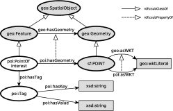
(a) Ontology for Points of Interest

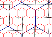
(b) Visualization of the geometric part of the synthetic dataset

Figure 1: Synthetic dataset

The workload generator produces synthetic datasets of arbitrary size that resemble features on a map. As in VESPA [14], the produced datasets model the following geographic features: states in a country, land ownership, roads and points of interest. For each dataset, we developed a minimal ontology that follows a general version of the schema of OpenStreetMap and uses GeoSPARQL ontologies and vocabularies. In Figure 1(a) we present the developed ontology for representing points of interest only. As in [2, 8], every feature (i.e., point of interest) is assigned a number of thematic tags each of which consists of a key-value pair of strings. Each feature is tagged with key $1$, every other feature with key $2$, every fourth feature with key $4$, etc. up to key $2^{k},k\in\mathbb{N}$. This tagging makes it possible to select different parts of the entire dataset in a uniform way, and perform queries of various thematic selectivities. For example, if we selected all points of interest tagged with key $1$, we would select all available points of interest, if we selected all points of interest tagged with key $2$, we would select half of them, etc.

Every feature has a spatial extent as well that is modelled using the GeoSPARQL vocabulary. The spatial extent of the land ownership dataset constitutes a uniform grid of $n\times n$ hexagons. The land ownership dataset forms the basis for the spatial extent of all generated datasets since the size of each dataset is given relatively to the number $n$. By modifying the number of hexagons along an axis, we produce datasets of arbitrary size. As we will see in the following section, this enabled us to adjust the selectivity of the spatial predicates appearing in queries in a uniform way too.

As in [14], the generated land ownership dataset consists of $n^{2}$ features with hexagonal spatial extent, where each hexagon is placed uniformly on a $n\times n$ grid. The cardinality of the land ownerships is $n^{2}$. The generated state dataset consists of $(\frac{n}{3})^{2}$ features with hexagonal spatial extent, where each hexagon is placed uniformly on a $\frac{n}{3}\times\frac{n}{3}$ grid. The cardinality of the state geometries is $(\frac{n}{3})^{2}$. The generated road dataset consists of $n$ features with sloping line gometries. Half of the line geometries are roughly horizontal and the other half are roughly vertical. Each line consists of $\frac{n}{2}+1$ line segments. The cardinality of the road geometries is $n$. The generated point of interest dataset consists of $n^{2}$ features with point geometries which are uniformly placed on $n$ sloping, evenly spaced, parallel lines. The cardinality of the point of interest geometries is $n^{2}$. In Figure 1(b) we present a sample of the generated geometries.

3.2.2 Queries.

Table 4: Query templates for generating SPARQL queries corresponding to (a) spatial selections, and (b) spatial joins.

SELECT ?s

WHERE {

?s ns:hasGeometry/ns:asWKT ?g.

?s c:hasTag/ns:hasKey "THEMA".

FILTER(FUNCTION(?g, "GEOM"))}

SELECT ?s1 ?s2

WHERE {

?s1 ns1:hasGeometry/ns1:asWKT ?g1.

?s1 ns1:hasTag/ns1:hasKey "THEMA".

?s2 ns2:hasGeometry/ns2:asWKT ?g2.

?s2 ns2:hasTag/ns2:hasKey "THEMA’".

FILTER(FUNCTION(?g1, ?g2))}

The synthetic workload generator produces SPARQL queries corresponding to spatial selection and spatial joins by instantiating the two query templates presented in Table 4.

The query template used for producing SPARQL queries corresponding to spatial selections is identical to the query template used in [2, 8]. In this query template, parameter THEMA is one of the values used when assigning tags to a feature and parameter GEOM is the WKT serialization of a rectangle. As in [8], we define the thematic selectivity of an instantiation of the query template as the fraction of the total features of a dataset that are tagged with a key equal to THEMA. For example, by altering the value of THEMA from 1 to 2, we reduce the thematic selectivity of the query by selecting half the nodes we previously did. We define the spatial selectivity of an instantiation of the query template as the fraction of the total features for which the topological relations defined by parameter FUNCTION holds between each of them and the rectangle defined by parameter GEOM. By modifying the value of the parameter namespace ns we specify the dataset and the corresponding type of geometric information that is examined by an instance of the query template.

The query template used for producing SPARQL queries corresponding to spatial joins involves two datasets identified by the values of the parameter namespaces ns1 and ns2. In this query template as well, parameters THEMA and THEMA’ control the thematic selectivity of the query. The value of parameter FUNCTION defines the topological relation that must hold between instances of the two datasets that are involved in an instance of the query template. For example, by instantiating the query template (b) with the values poi for ns1, state for ns2, 1 for THEMA, 2 for THEMA’ and geof:sfWithin for FUNCTION, we get a SPARQL query that asks for all generated points of interest that are inside half of the generated states.

These query templates allow us to generate SPARQL queries with great diversity regarding their spatial and thematic selectivity, thus stressing the optimizers of the geospatial RDF stores that we test and evaluating their effectiveness in identifying efficient query plans.

4 Benchmark Results

In this section we present the results of running Geographica against three open source RDF stores. As we mentioned earlier, we chose to test the systems Strabon, Parliament and uSeekM that currently provide support for a rich subset of GeoSPARQL and stSPARQL.

4.1 Experimental Setup

In this section we describe the setup of the experiments used to evaluate the selected triple stores. The machine that was used to run the benchmark is equipped with two Intel Xeon E5620 processors with 12MB L3 cache running at 2.4 GHz, 24 GB of RAM and a RAID-5 disk array that consists of four disks. Each disk has 32 MB of cache and its rotational speed is 7200 rpm.

Each query in the micro and the synthetic benchmark was run three times on cold and warm caches. For warm caches, we ran each query once before measuring the response time, in order to warm up the caches. We measured the response time for each query posed by measuring the elapsed time from submitting the query until a complete iteration over the results had been completed. The response time of each query was measured and the median of all measurements is reported. A timeout of one hour is set as a time limit for all queries. For the macro benchmark, we run each scenario many times (with different initialization each time) for one hour without cleaning the caches and we report the average time for a complete execution of all queries defined in each scenario. Strabon and uSeekM utilize Postgres enhanced with PostGIS as a spatially-enabled relational backend. For these systems, we set up an instance of Postgres 9.2 with PostGIS 2.0 and we tuned it to make better use of the system resources.

For every dataset of Geographica, a unique property is used to connect geometries with their serialization (e.g. the Corine Land Use/Land cover ontology defines the property clc:asWKT), and this property is defined as a subproperty of the property geo:asWKT that is defined by GeoSPARQL. Parliament is able to identify and index a triple that represents the serialization of a geometric object only when the property geo:asWKT is used. As a result, the RDFS reasoning capabilities of Parliament have to be enabled so that it performs forward chaining during data loading and indexes the geometry using the spatial index as well. Strabon and uSeekM do not perform any reasoning on the input data.

4.2 Real-World Workload

4.2.1 Dataset Storage.

In this section we present the time required by each system to store and index the datasets of the real-world workload. As shown in Table 5, Strabon requires a lot of time to store and index the real-world dataset. Stabon heavily indexes the produced DBMS tables since the existence of named graphs require the creation of additional multi-column indices, thus leading to increased indexing time. uSeekM needs less time since it is based on the native repository of Sesame which is known to be the most efficient implementation of Sesame for average sized datasets. Since Parliament provides RDFS inference capabilities, it is reasonably slower that uSeekM as it requires more time to perform forward chaining on the input dataset.

Workload	Strabon	uSeekM	Parliament
Real-world	550 sec.	214 sec.	250 sec.
Synthetic	221 sec.	406 sec.	462 sec.

Table 5: Storing times

4.2.2 Micro Benchmark.

The results of the micro benchmark are shown in Figure 2 where the response time of each query is reported for both cold and warm caches.

First, results about computing non-topological functions are reported. For this class of queries uSeekM performs the best. Both uSeekM and Strabon are extensions of Sesame, but uSeekM extends the native store of Sesame which is known to be more efficient, for small datasets, than Sesame implementations on top of a DBMS, like Strabon, thus the performance gain. Computing the area of polygons (Query 6) was tested only in uSeekM and Strabon since Parliament does not offer such functionality. Finally, comparing the performance of all systems in cold and warm caches, we observe that none of the RDF stores exploits the warm caches when evaluating topological functions. This is because the non-topological functions used in this set of queries are computationally intensive (especially when complex geometries are used) and the time spent in CPU usage dominates I/O time.

Both uSeekM and Strabon utilize PostGIS for evaluating the spatial part of a query. Thus the performance of uSeekM and Stabon is comparable regarding selections. Strabon performs slightly better than uSeekM in cold caches, but uSeekM improves its performance on warm caches and outperforms Strabon. Parliament, in general, needs an order of magnitude more time than Strabon and uSeekM. It is interesting to have a closer look at Queries 14 and 15 which are semantically equivalent. Both ask for points that have a given distance from a given point. However, Query 14 creates the buffer of a given point with radius $r$ and asks for points which are within this buffer, while Query 15 asks for points that have distance less than $r$ from the given point. Parliament and uSeekM perform better in Query 15 which does not require buffer computation than in Query 14. However, Strabon performs the same in both queries in cold caches while in warm caches it answers Query 14 faster than the other two systems.

In the case of spatial joins, uSeekM and Parliament are able to evaluate only queries 18 and 27 given the time limit of one hour. Parliament evaluates separately graph patterns corresponding to different graphs, produces the Cartesian product between them, and then applies the spatial predicate to the result of the Cartesian product. This strategy is very costly, thus Parliament is not able to answer any spatial join given the time limit. uSeekM does not utilize PostGIS in cases of joins, but only for spatial selections, so Strabon, which fully exploits the query engine of PostGIS outperforms uSeekM. In all cases, warm caches do not affect the response time of the queries since a large number of intermediate results is produced. Finally, spatial aggregations are tested. Strabon is the only system that supports spatial aggregates so we do not have any comparison here. The only thing to notice then is that Query 28 which simply computes the minimum bounding box that contains all geometries of the GAG dataset, is much faster than Query 29 which computes the union of the same geometries.

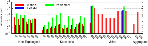
(a) Cold caches

(b) Warm caches

Figure 2: Response times, real-world workload

4.2.3 Macro Benchmark.

The results of the macro benchmark are shown in Table 6. In this table we report the average time needed for a complete iteration of all the queries of each scenario. The Reverse Geocoding scenario has two queries which use the function distance with a fixed limit. uSeekM performs the best in this scenario while Strabon needs an order of magnitude more time. The Map Search and Browsing scenario has one thematic query and two queries which select points and lines in a given rectangle. Strabon and uSeekM have similar performance in this scenario while Parliament needs an order of magnitude more time. Finally, the Rapid Mapping for Fire Monitoring scenario is the most demanding scenario. It comprises three queries that return lines and polygons that are located inside a given rectangle, and two complex queries which include spatial joins and construct new geometries (boundary and intersection) on the fly. Only Strabon can serve this scenario since uSeekM and Parliament needed more than an hour to evaluate the query RM6.

Scenario	Strabon	uSeekM	Parliament
Reverse Geocoding	65s	0.77s	2.6s
Map Search and Browsing	0.9s	0.6s	22.2
Rapid Mapping for Fire Monitoring	207.4s	-	-

Table 6: Average Iteration times - Macro Scenarios

4.3 Synthetic Workload

Let us now discuss representative experiments that we run using a synthetic workload that was produced using the generator presented in Section 3. We generated a dataset by setting $n=512$ and $k=9$, where $n$ is the number used for defining the cardinalities of the generated geometries, and $k$ is the number used for defining the cardinalities of the generated tag values. This instantiation of the synthetic generator produces $262,144$ land ownership instances, $28,900$ states, $512$ roads and $262,144$ points of interest. Each feature is tagged with key $1$, every other feature with key $2$, etc. up to key $512$. The resulting dataset consists of 3,880,224 triples and its size is 745 MB.

4.3.1 Dataset Storage.

Table 5 presents the time required by each system to store and index the synthetic dataset. uSeekM requires more time than Strabon for storing the dataset, since it stores it in a Sesame native store and then it stores triples with geometric information at PostGIS as well. This overhead is significant compared to the total time required for storing the dataset, but leads to better response times in some cases. As we have already explained in Section 4.2.1, Parliament needs more time to store the synthetic dataset as well for the real-world workload because it performs forward chaining on the input dataset.

4.3.2 Queries.

We instantiated the query template presented in Table 4 in order to produce SPARQL queries corresponding to spatial selections that ask for land ownerships that intersect a given rectangle, and points of interest that are within a given recangle. The given rectangle is generated in such as a way that the spatial predicate of the query holds for 1‱, 10%, 25%, 50%, 75% or all the features of the respective dataset. In addition, we instantiated the query template using the extreme values 1 and 512 of the parameter THEMA for selecting either all or approximatly 2‱ of the total features of a dataset. The response time of each system for evaluating the instantiations of this query template are presented in Figures 3(a)-3(h).

We instantiated the query template presented in Table 4 in order to produce SPARQL queries corresponding to spatial joins that ask for land ownerships that intersect a state, touching states and points of interest that are located inside a state. We also instantiated this query template using all combinations of the extreme values 1 and 512 for the parameters THEMA and THEMA’. The response time of each system for evaluating the instantiations of this query template are presented in Figures 3(i)-3(k).

By examining Figures 3(a)- 3(h), we observe that Strabon has very good performance overall. Strabon pushes the evaluation of a SPARQL query to the underlying spatially-enabled DBMS, which in this case is Postgres enhanced with PostGIS. PostGIS has recently been enhanced with selectivity estimation capabilities. As a result, when a query selects only a few geometries, query evaluation always starts with the evaluation of the spatial predicate using the spatial index, thus resulting in few intermmediate results and good response times. While the spatial selectivity increases and more geometries satisfy the spatial predicate, the optimizer of Postgres chooses different query plans. For example, when the value of the parameter THEMA is $1$ (Figures 3(a), 3(c), 3(e), 3(g)) and the value of the parameter GEOM is such that all geometries satisfy the spatial predicate, Postgres ignores the spatial index and performs a sequential scan on the table storing the geometries for evaluating the spatial predicate. Similarly, when the value of the parameter THEMA is $512$ (Figures 3(b), 3(d), 3(f), 3(h)) and the value of the parameter GEOM is such that all geometries satisfy the spatial predicate, Postgres starts with the evaluation of the thematic selection that produces few intermediate results since only 2‱ of the features satisfy the thematic predicate, resulting in good query response times. In the case of spatial joins (Figures 3(i)- 3(k)), Strabon is the fastest system in most cases. The optimizer of Postgres takes into account the thematic selectivity of the queries and selects good query plans, thus Strabon is the only system that is able to answer the spatial joins given the one hour timeout when the parameters THEMA and THEMA’ are equal to $1$.

Regarding uSeekM, we observe that its performance is not affected by the thematic selectivity of the query. For spatial selections, uSeekM always start by evaluating the spatial predicate in PostGIS and then continues the query evaluation in the native Sesame store. As a result, regardless of the thematic selectivity, the response time of uSeekM increases while increasing the number of features with geometies that satisfy the given spatial predicate.

Regarding Parliament, we observe that its performance is not affected neither by the thematic nor by the spatial selectivity of a query. Parliament always starts by evaluating the non-spatial part of a query and then applies the thematic filter and evaluates the spatial predicate exhaustively on the intermediate results. Thus, the thematic and spatial selectivity of a query do not affect the response time of Parliament.

In the case of spatial joins, uSeekM and Parliament produces the Cartesian product between the graph patterns that are joined through the spatial predicate, and evaluate the spatial predicate afterwards. This strategy is very costly, thus Parliament is not able to answer most spatial joins given the one hour timeout and uSeekM is more than two orders of magnitude slower than Strabon. However, in Figure 3(j) we observe that uSeekM outperforms Strabon. Strabon stores all geometries in a single table, so the evaluation of the spatial predicate $Touches$ on this table returns not only the geometries of states that touch each other, but the touching geometries of land ownerships as well. The touching geometries of land ownerships are discarded later on, but this overhead proves to be more costly than producing a Cartesian product and evaluating the spatial predicate afterwards.

5 Conclusions

We presented a benchmark for evaluating the performance of geospatial RDF stores that are beginning to emerge. We defined two workloads that test on the one hand the performance of the spatial component of such systems in isolation, and on the other hand test whether spatial query processing is deeply integrated in their query engines.

(a) Intersects tag 1, cold caches

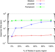
(b) Intersects tag 512, cold caches

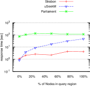
(c) Within tag 1, cold caches

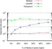
(d) Within tag 512, cold caches

(e) Intersects tag 1, warm caches

(f) Intersects tag 512, warm caches

(g) Within tag 1, warm caches

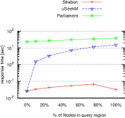
(h) Within tag 512, warm caches

(i) Intersects

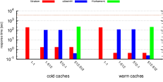
(j) Touches

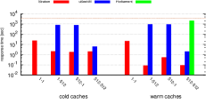
(k) Within

Figure 3: Response times - Synthetic Workload

References

- [1] Bizer, C., Schultz, A.: The Berlin SPARQL Benchmark. In: IJSWIS. vol. 5 (2009)
- [2] Brodt, A., Nicklas, D., Mitschang, B.: Deep Integration of Spatial Query Processing into Native RDF Triple Stores. In: SIGSPATIAL (2010)
- [3] Gunther, O., Picouet, P., Saglio, J.M., Scholl, M., Oria, V.: Benchmarking Spatial Joins À La Carte. In: IJGIS. vol. 13 (1999)
- [4] Guo, Y., Pan, Z., Heflin, J.: LUBM: A Benchmark for OWL Knowledge Base Systems. In: Web Semantics. vol. 3 (2005)
- [5] Kolas, D.: A Benchmark for Spatial Semantic Web Systems. In: International Workshop on Scalable Semantic Web Knowledge Base Systems (2008)
- [6] Koubarakis, M., Kontoes, C., Manegold, S., Karpathiotakis, M., Kyzirakos, K., Bereta, K., Garbis, G., Nikolaou, C., Michail, D., Papoutsis, I., Herekakis, T., Ivanova, M., Zhang, Y., Pirk, H., Kersten, M., Dogani, K., Giannakopoulou, S., Smeros, P.: Real-Time Wildfire Monitoring Using Scientific Database and Linked Data Technologies. In: EDBT (2013)
- [7] Koubarakis, M., Karpathiotakis, M., Kyzirakos, K., Nikolaou, C., Sioutis, M.: Data Models and Query Languages for Linked Geospatial Data. In: Reasoning Web. Semantic Technologies for Advanced Query Answering. LNCS (2012)
- [8] Kyzirakos, K., Karpathiotakis, M., Koubarakis, M.: Strabon: A Semantic Geospatial DBMS. In: ISWC (2012)
- [9] Morsey, M., Lehmann, J., Auer, S., Ngomo, A.C.N.: DBpedia SPARQL Benchmark - Performance Assessment with Real Queries on Real Data. In: ISWC (2011)
- [10] Mpereta, K., Smeros, P., Koubarakis, M.: Representing and Querying the valid time of triples for Linked Geospatial Data. In: ESWC (2013)
- [11] Myllymaki, J., Kaufman, J.H.: DynaMark: A Benchmark for Dynamic Spatial Indexing. In: Mobile Data Management. vol. 2574 (2003)
- [12] Open Geospatial Consortium: OGC GeoSPARQL - A geographic query language for RDF data. OGC Implementation Standard (2012)
- [13] Patel, J., Yu, J., Kabra, N., Tufte, K., Nag, B., Burger, J., Hall, N., Ramasamy, K., Lueder, R., Ellmann, C., Kupsch, J., Guo, S., Larson, J., De Witt, D., Naughton, J.: Building a Scaleable Geo-Spatial DBMS: Technology, Implementation, and Evaluation. In: ACM SIGMOD (1997)
- [14] Paton, N.W., Williams, M.H., Dietrich, K., Liew, O., Dinn, A., Patrick, A.: VESPA: A Benchmark for Vector Spatial Databases. In: BNCOD (2000)
- [15] Ray, S., Simion, B., Demke Brown, A.: Jackpine: A Benchmark to Evaluate Spatial Database Performance. In: ICDE (2011)
- [16] Schmidt, M., Hornung, T., Lausen, G., Pinkel, C.: SP2Bench: A SPARQL Performance Benchmark. In: ICDE (2009)
- [17] Stonebraker, M., Frew, J., Gardels, K., Meredith, J.: The SEQUOIA 2000 Storage Benchmark. In: ACM SIGMOD (1993)