Locking Free Quadrilateral Continuous/Discontinuous Finite Element Methods for the Reissner–Mindlin Plate

Abstract

We develop a finite element method with continuous displacements and discontinuous rotations for the Mindlin-Reissner plate model on quadrilateral elements. To avoid shear locking, the rotations must have the same polynomial degree in the parametric reference plane as the parametric derivatives of the displacements, and obey the same transformation law to the physical plane as the gradient of displacements. We prove optimal convergence, uniformly in the plate thickness, and provide numerical results that confirm our estimates.

1 Introduction

The Reissner-Mindlin Plate Model and Shear Locking.

The Reissner-Mindlin equations is a model of the displacement of a moderately thick plate under transversal load. The unknows are the normal displacement field $u$ and the rotation field ${\boldsymbol{\theta}}$ of a normal fiber. The difficulty with this model, from a numerical point of view, is the matching of the approximating spaces for ${\boldsymbol{\theta}}$ and $u$. As the thickness $t\rightarrow 0$, the difference $\nabla u-{\boldsymbol{\theta}}$ must tend to zero, which, for naive choices of spaces, leads to a deterioration of the approximation known as locking or in this case shear locking since the difficulty emanates from the term involving the shear energy. The situation is particularly difficult if we wish to use low order approximations.

Earlier Work.

There are basically three different approaches to solve this problem. Perhaps the most common approach has been to use a projection to relax the equation, which essentially corresponds to a mixed formulation where an additional variable, often the shear vector proportional to $(\nabla u-{\boldsymbol{\theta}})/t^{2}$, is introduced. For instance, the MITC element family of Bathe and co-workers [6] are based on this approach. For quadrilaterals, this type of approach has been used and analyzed in [2, 14, 15, 21, 22].

Another approach is to use a stabilized mixed formulation, see Chapelle and Stenberg, [11, 12].

Finally, a third approach is to use finite element spaces that are rich enough to satisfy the shear constraint exactly while maintaining optimal approximation properties. This approach was first proposed by Hansbo and Larson [20], where continuous piecewise quadratics for the displacements and discontinuous piecewise linears for the rotations in a discontinuous Galerkin formulation. Further developments, still using simplicial elements, were given by Arnold et al. [4], Heintz et al. [18], and Bösing et al. [8]. When the thickness of the plate tends to zero we obtain the Kirchhoff plate and our scheme can be seen as a version of the method proposed in [16], see [18]. In this context we also mention the fully discontinuous Galerkin method developed in [19] and the parametric continuous/discontinuous Galerkin method [9] for the Kirchhoff plate.

New Contributions.

In this paper we extend the method of [20] to quadrilateral elements. We show that, with the proper definition of the finite element space for the rotations, we can satisfy the equation $\nabla u-{\boldsymbol{\theta}}=0$ exactly while maintaining optimal approximation properties and thus together with stability we obtain optimal a priori error estimates uniformly in the thickness parameter. Using continuous tensor product quadratics for the displacements the suitable space for the rotations consists of discontinuous parametric vector polynomials that are also mapped in the same way as the gradient of elements. The mapping is the rotated, or covariant, Piola mapping that preserves tangent traces, and naturally appears in the context of curl conforming elements, see [17]. We could also use the smaller subspace of tangentially continuous functions for the rotations instead of the full discontinuous space. The interpolation error estimates on quadrilaterals are based on the observation that tensor product polynomials mapped with a bilinear map contain complete polynomials, cf. [1, 3], and thus the estimates follows from the Bramble–Hilbert lemma and scaling. We also show that the condition required to avoid locking also implies that complete linear polynomials are contained in the space for the rotations. Our analysis is remarkably simple and avoids difficulties caused by the mixed formulations and basically rely on proper construction of the discrete spaces and approximation properties that takes advantage of the stability of the underlying continuous problem.

We remark that the idea of using covariant maps to obtain suitable approximations of the rotations has also recently been used in the context of isogeometric approximations by Beirão da Veiga, Buffa, Lovadina, Martinelli, and Sangalli [7].

Outline.

In Section 2 we formulate the Reissner–Mindlin model on weak form, in Section 3 we introduce the quadrilateral finite element spaces and formulate the finite element method, in Section 4 we derive approximation properties and a priori error estimates, and in Section 5 we present numerical results illustrating the theoretical results.

2 The Reissner-Mindlin Plate Model

2.1 Energy Functional

Consider a plate with thickness $t$ occupying a convex polygonal domain $\Omega$ in ${{\mathbb{R}}}^{2}$, which is clamped at the boundary $\partial\Omega$. The Reissner-Mindlin plate model can be derived from minimization of the sum of the bending energy, the shear energy, and the potential of the surface load

$${\mathcal{E}_{\text{RM}}}(u,{\boldsymbol{\theta}}):=\frac{1}{2}a({\boldsymbol{\theta}},{\boldsymbol{\theta}})+\frac{\kappa}{2\,t^{2}}\int_{\Omega}|\nabla u-{\boldsymbol{\theta}}|^{2}\,d\Omega-\int_{\Omega}g\,u\,d\Omega$$ (1)

Here $u$ is the transverse displacement, ${\boldsymbol{\theta}}$ is the rotation of the median surface, $t$ is the thickness, $t^{3}\,g$ is the transverse surface load, and the bending energy $a(\cdot,\cdot)$ is defined by

$$a({\boldsymbol{\theta}},{\boldsymbol{\vartheta}}):=\int_{\Omega}\Bigl{(}2\mu{\boldsymbol{\varepsilon}}({\boldsymbol{\theta}}):{\boldsymbol{\varepsilon}}({\boldsymbol{\vartheta}})+\lambda\nabla\cdot{\boldsymbol{\theta}}\,\nabla\cdot{\boldsymbol{\vartheta}}\Bigr{)}\,d\Omega$$ (2)

where ${\boldsymbol{\varepsilon}}$ is the curvature tensor

$${\boldsymbol{\varepsilon}}({\boldsymbol{\theta}}):=\left[\begin{array}[]{>{\displaystyle}c>{\displaystyle}c}\frac{\partial\theta_{x}}{\partial x}&\frac{1}{2}\left(\frac{\partial\theta_{x}}{\partial y}+\frac{\partial\theta_{y}}{\partial x}\right)\\[11.38109pt] \frac{1}{2}\left(\frac{\partial\theta_{x}}{\partial y}+\frac{\partial\theta_{y}}{\partial x}\right)&\frac{\partial\theta_{y}}{\partial y}\end{array}\right].$$ (3)

The material parameters are given by the relations $\kappa=E\,k/(2(1+\nu))$, $\mu:=E/(24(1+\nu))$, and $\lambda:=\nu E/(12(1-\nu^{2}))$, where $E$ and $\nu$ are the Young’s modulus and Poisson’s ratio, respectively, and $k$ is a shear correction factor. We shall alternatively write the bending energy product as

$$a({\boldsymbol{\theta}},{\boldsymbol{\vartheta}})=\int_{\Omega}{\boldsymbol{\sigma}}({\boldsymbol{\theta}}):{\boldsymbol{\varepsilon}}({\boldsymbol{\vartheta}})\,d\Omega$$ (4)

where ${\boldsymbol{\sigma}}({\boldsymbol{\theta}}):=2\mu{\boldsymbol{\varepsilon}}({\boldsymbol{\theta}})+\lambda\nabla\cdot{\boldsymbol{\theta}}\,{\boldsymbol{1}}$ is the moment tensor.

2.2 Weak Form

The transverse displacement and rotation vector are solutions to the following variational problem: find $(u,{\boldsymbol{\theta}})\in H_{0}^{1}(\Omega)\times[H_{0}^{1}(\Omega)]^{2}$ such that

$$a({\boldsymbol{\theta}},{\boldsymbol{\vartheta}})+\frac{\kappa}{t^{2}}(\nabla u-{\boldsymbol{\theta}},\nabla v-{\boldsymbol{\vartheta}})=(g,v),\quad\forall(v,{\boldsymbol{\vartheta}})\in H_{0}^{1}(\Omega)\times[H_{0}^{1}(\Omega)]^{2}$$ (5)

where $(\cdot,\cdot)$ denotes the $L^{2}(\Omega)$ inner product, $H^{k}(\Omega)$ are the usual Sobolev spaces, and the functions in $H^{1}_{0}(\Omega)$ have zero trace on the boundary $\partial\Omega$.

3 The Finite Element Method

3.1 The Quadrilateral Mesh

Next, let $\mathcal{K}^{h}=\{K\}$ be a family of quasiuniform partitions of $\Omega$ into convex quadrilaterals $K={\boldsymbol{F}}_{K}(\widehat{K})$ with mesh parameter $h$ such that $ch\leq h_{K}\leq Ch$, where $h_{K}=\text{diam}(K)$, for all $K\in\mathcal{K}^{h}$. We also assume that $\mathcal{K}^{h}$ is a shape regular partition in the sense that $h_{K}/\rho_{K}\leq C$ for all $K\in\mathcal{K}^{h}$, where $\rho_{K}$ is the smallest diameter of the largest inscribed circle in any of the four subtriangles obtained by inserting a diagonal between two opposite corners in $K$.

3.2 Parametric Elements for Displacements and Rotations

In order to define our finite element spaces we begin with a continuous parametric finite element space $V_{\rm D}^{h}$ for the displacement $u$ and then we determine a space ${\boldsymbol{V}}_{\rm R}^{h}$ of discontinuous piecewise parametric functions for the rotations ${\boldsymbol{\theta}}$ such that

$$\nabla V_{\rm D}^{h}\subseteq{\boldsymbol{V}}_{\rm R}^{h}$$ (6)

in order to be able to satisfy the equation ${\boldsymbol{\theta}}-\nabla u=0$ exactly, when the thickness tends to zero. Using this inclusion we identify the proper space for the rotations. For clarity, we restrict the presentation to quadratic tensor product approximation of the displacements. extension to higher order elements follow directly.

3.2.1 Displacements

Let $\widehat{K}$ be the reference unit square and $Q_{k,l}(\widehat{K})$ the space of tensor product polynomials of order $k$ and $l$ in each variable, more precisely

$$Q_{k,l}(\widehat{K}) =\text{span}\{\widehat{x}^{\alpha}\widehat{y}^{\beta}\;:\;0\leq\alpha\leq k,0\leq\beta\leq l\}$$ (7)

and $Q_{k}(\widehat{K})=Q_{k,k}(\widehat{K})$. For each $K\in\mathcal{K}^{h}$ let ${\boldsymbol{F}}_{K}:\widehat{K}\rightarrow{\bf R}^{2}$ be the bilinear, i.e., ${\boldsymbol{F}}_{K}\in[Q_{1}(\widehat{K})]^{2}$, mapping such that $K={\boldsymbol{F}}_{K}(\widehat{K})$. We define the space of parametric tensor product polynomials on $K$ by

$$V_{{\rm D},K}=\{p:K\rightarrow{\bf R}\,:\,p=\widehat{p}\circ{\boldsymbol{F}}_{K}^{-1}\}$$ (8)

and the corresponding space on $\mathcal{K}^{h}$ of continuous piecewise parametric tensor product polynomials

$$V^{h}_{\rm D}=\{v:\Omega\rightarrow{\boldsymbol{R}}:v|_{K}\in V_{{\rm D},K}\;\forall K\in\mathcal{K}^{h},v\in C(\Omega)\}$$ (9)

3.2.2 Rotations

Turning to the space for the rotations we recall that, since $p=\widehat{p}\circ{\boldsymbol{F}}_{K}^{-1}$, we have

$$\nabla p(x)=DF^{-\rm{T}}_{K}\widehat{\nabla}\widehat{p}(\widehat{x})=DF^{-\rm{T}}_{K}\widehat{\nabla}\widehat{p}({\boldsymbol{F}}^{-1}_{K}(x))$$ (10)

where $\widehat{\nabla}$ is the gradient in the reference coordinates. Introducing the rotated or covariant Piola mapping

$${\boldsymbol{R}}_{K}:\widehat{{\boldsymbol{V}}}_{\rm R}\ni\widehat{{\boldsymbol{\theta}}}\mapsto D{\boldsymbol{F}}^{-{\rm T}}_{K}\widehat{{\boldsymbol{\theta}}}\circ{\boldsymbol{F}}_{K}^{-1}\in{{\boldsymbol{V}}_{\rm R}}$$ (11)

we have $\nabla p(x)=DF^{-\rm{T}}_{K}\widehat{\nabla}\widehat{p}(\widehat{x})={\boldsymbol{R}}_{K}\widehat{\nabla}\widehat{p}(\widehat{x})$. We are thus led to defining the following space for the rotations

$${\boldsymbol{V}}_{{\rm R},K}={\boldsymbol{R}}_{K}{\widehat{{\boldsymbol{V}}}}_{\rm R}$$ (12)

where ${\widehat{{\boldsymbol{V}}}}_{\rm R}$ is a space on the reference unit square $\widehat{K}$ that satisfies

$$\widehat{\nabla}{\widehat{V}}_{{\rm D},K}=Q_{1,2}(\widehat{K})\times Q_{2,1}(\widehat{K})\subseteq\widehat{{\boldsymbol{V}}}_{{\rm R},K}$$ (13)

We finally define the space of discontinuous mapped parametric functions

$${\boldsymbol{V}}^{h}_{\rm R}=\{{\boldsymbol{\theta}}:\Omega\rightarrow{{\boldsymbol{R}}}^{2}:{\boldsymbol{v}}|_{K}\in{\boldsymbol{V}}_{{\rm R},K}\;\forall K\in\mathcal{K}^{h}\}$$ (14)

Remark 3.1

We note that it is indeed also possible to chose a subspace of ${\boldsymbol{V}}^{h}_{\rm R}$ that consists of functions that have continuous tangential trace at each edge. This case is also covered by our analysis and basically only depends on the choice of interpolation operator on the reference element.

3.3 The Finite Element Method

Let $\mathcal{E}^{h}=\{E\}$ be the set of edges in the mesh $\mathcal{K}^{h}$. We split $\mathcal{E}^{h}$ into two disjoint subsets

$$\mathcal{E}^{h}=\mathcal{E}^{h}_{I}\cup\mathcal{E}^{h}_{B}$$ (15)

where $\mathcal{E}^{h}_{I}$ is the set of edges in the interior of $\Omega$ and $\mathcal{E}^{h}_{B}$ is the set of edges on the boundary $\partial\Omega$. Further, with each edge we associate a fixed unit normal ${\boldsymbol{n}}$ such that for edges on the boundary ${\boldsymbol{n}}$ is the exterior unit normal. We denote the jump of a function ${\boldsymbol{v}}\in{\boldsymbol{V}}_{\rm R}^{h}$ at an edge $E$ by $\left[{\boldsymbol{v}}\right]={\boldsymbol{v}}^{+}-{\boldsymbol{v}}^{-}$ for $E\in\mathcal{E}^{h}_{I}$ and $\left[{\boldsymbol{v}}\right]={\boldsymbol{v}}^{+}$ for $E\in\mathcal{E}^{h}_{B}$, and the average $\langle{\boldsymbol{v}}\rangle=({\boldsymbol{v}}^{+}+{\boldsymbol{v}}^{-})/2$ for $E\in\mathcal{E}^{h}_{I}$ and $\langle{\boldsymbol{v}}\rangle={\boldsymbol{v}}^{+}$ for $E\in\mathcal{E}^{h}_{B}$, where ${\boldsymbol{v}}^{\pm}({\boldsymbol{x}})=\lim_{\epsilon\downarrow 0}{\boldsymbol{v}}({\boldsymbol{x}}\mp\epsilon\,{\boldsymbol{n}})$ with ${\boldsymbol{x}}\in E$.

The method takes the form: find $(u^{h},{\boldsymbol{\theta}}^{h})\in V^{h}_{\rm D}\times{\boldsymbol{V}}^{h}_{\rm R}$ such that

$$a_{h}({\boldsymbol{\theta}}^{h},{\boldsymbol{\vartheta}})+\frac{\kappa}{t^{2}}\left(\nabla u^{h}-{\boldsymbol{\theta}}^{h},\nabla v-{\boldsymbol{\vartheta}}\right)=(g,v)\quad\forall(v,{\boldsymbol{\vartheta}})\in V^{h}_{\rm D}\times{\boldsymbol{V}}^{h}_{\rm R}$$ (16)

Here the bilinear form $a_{h}(\cdot,\cdot)$ is defined by

$$\begin{array}[]{>{\displaystyle}l>{\displaystyle}l}a_{h}({\boldsymbol{\theta}}^{h},{\boldsymbol{\vartheta}})&=\sum_{K\in\mathcal{K}^{h}}({\boldsymbol{\sigma}}({\boldsymbol{\theta}}^{h}),{\boldsymbol{\varepsilon}}({\boldsymbol{\vartheta}}))_{K}\\ &\quad-\sum_{E\in\mathcal{E}^{h}_{I}\cup\mathcal{E}^{h}_{B}}(\langle{\boldsymbol{n}}\cdot{\boldsymbol{\sigma}}({\boldsymbol{\theta}}^{h})\rangle,[{\boldsymbol{\vartheta}}])_{E}+(\langle{\boldsymbol{n}}\cdot{\boldsymbol{\sigma}}({\boldsymbol{\vartheta}})\rangle,[{\boldsymbol{\theta}}^{h}])_{E}\\ &\quad+(\mu+\lambda)\,\gamma\sum_{E\in\mathcal{E}^{h}_{I}\cup\mathcal{E}^{h}_{B}}(h_{E}^{-1}[{\boldsymbol{\theta}}^{h}],[{\boldsymbol{\vartheta}}])_{E}\end{array}$$

where $\gamma$ is a positive constant, $h_{E}$ is defined by

$$h_{E}=\left(|T^{+}|+|T^{-}|\right)/(2\,|E|)\quad\text{for $E=\partial T^{+}\cap\partial T^{-}$}$$ (17)

with $|K|$ the area of $K$, on each edge, and $(\cdot,\cdot)_{\omega}$ is the $L^{2}(\omega)$ inner product with $\omega=K,E$.

4 A Priori Error Estimates

The analysis presented here extends the analysis in Hansbo and Larson [20] to parametric elements on quadrilaterals. For completeness we include the necessary results but refer to [20] and [18], for further details.

4.1 Stability and Continuity of the Discrete Bilinear Form

Let the mesh dependent energy-like norm, associated with the bilinear form $a_{h}(\cdot,\cdot)$ be defined by

$$|\|{\boldsymbol{\vartheta}}\||^{2}= \sum_{K\in\mathcal{K}^{h}}({\boldsymbol{\sigma}}({\boldsymbol{\vartheta}}),{\boldsymbol{\varepsilon}}({\boldsymbol{\vartheta}}))_{K}+\sum_{E\in\mathcal{E}^{h}}\frac{1}{2\mu+2\lambda}\|h_{E}^{1/2}\langle{\boldsymbol{n}}\cdot{\boldsymbol{\sigma}}({\boldsymbol{\vartheta}})\rangle\|_{E}^{2}$$ (18)

$$\qquad+\sum_{E\in\mathcal{E}^{h}}(2\mu+2\lambda)\|h_{E}^{-1/2}\left[{\boldsymbol{\vartheta}}\right]\|^{2}_{E}$$

We summarize the standard properties in the following and then state Cea’s lemma.

Lemma 4.1

It holds:

• Continuity: There is a constant $C$ such that

  $$a_{h}({\boldsymbol{\theta}},{\boldsymbol{\eta}})+\frac{\kappa}{t^{2}}(\nabla u-{\boldsymbol{\theta}},\nabla v-{\boldsymbol{\vartheta}})$$ (19)

  $$\qquad\leq C\left(|\|{\boldsymbol{\theta}}|\|^{2}+\frac{\kappa}{t^{2}}\|\nabla u-{\boldsymbol{\theta}}\|^{2}\right)^{\frac{1}{2}}\left(|\|{\boldsymbol{\eta}}|\|^{2}+\frac{\kappa}{t^{2}}\|\nabla v-{\boldsymbol{\vartheta}}\|^{2}\right)^{\frac{1}{2}}$$

  for all $(u,{\boldsymbol{\theta}}),(v,{\boldsymbol{\vartheta}})\in H^{1}_{0}(\Omega)\times([H^{1}_{0}(\Omega)]^{2}+{\boldsymbol{V}}_{\rm R}^{h})$.

• Coercivity: For $\gamma$ sufficiently large, there is a constant $m$ such that

  $$m\left(|\|{\boldsymbol{\theta}}|\|^{2}+\frac{\kappa}{t^{2}}\|\nabla u-{\boldsymbol{\theta}}\|^{2}\right)\leq a_{h}({\boldsymbol{\theta}},{\boldsymbol{\theta}})+\frac{\kappa}{t^{2}}(\nabla u-{\boldsymbol{\theta}},\nabla u-{\boldsymbol{\theta}})$$ (20)

  for all $(u,{\boldsymbol{\theta}})\in V^{h}_{\rm D}\times{\boldsymbol{V}}^{h}_{\rm R}$.

• Consistency: With $(u,{\boldsymbol{\theta}})$ the exact solution defined by (5) and $(u^{h},{\boldsymbol{\theta}}^{h})$ the discrete solution defined by (16) we have

  $$a_{h}({\boldsymbol{\theta}}-{\boldsymbol{\theta}}^{h},{\boldsymbol{\vartheta}})+\frac{\kappa}{t^{2}}(\nabla(u-u^{h})-({\boldsymbol{\theta}}-{\boldsymbol{\theta}}^{h}),\nabla v-{\boldsymbol{\vartheta}})=0$$ (21)

  for all $(v,{\boldsymbol{\vartheta}})\in V^{h}_{\rm D}\times{\boldsymbol{V}}^{h}_{\rm R}$.

Proof. The continuity estimate follows directly from Cauchy-Schwartz. The coercivity follows from coercivity for $a_{h}(\cdot,\cdot)$, which depend on the inverse inequality

$$\frac{1}{2\mu+2\lambda}\|h_{E}^{\frac{1}{2}}{\boldsymbol{\sigma}}({\boldsymbol{\vartheta}})\|^{2}_{\partial K}\leq C({\boldsymbol{\sigma}}({\boldsymbol{\vartheta}}),{\boldsymbol{\varepsilon}}({\boldsymbol{\vartheta}}))_{K}\quad\forall{\boldsymbol{\vartheta}}\in{\boldsymbol{V}}_{{\rm R},K}$$ (22)

This inequality is established by mapping to the reference element and using finite dimensionality and then mapping back in the same way as for affine elements. The consistency follows by using Green’s formula.

Lemma 4.2

(Cea’s Lemma) With $(u,{\boldsymbol{\theta}})$ the exact solution defined by (5) and $(u^{h},{\boldsymbol{\theta}}^{h})$ the discrete solution defined by (16) we have

$$|\|{\boldsymbol{\theta}}-{\boldsymbol{\theta}}^{h}|\|^{2}+\frac{\kappa}{t^{2}}\|\nabla(u-u^{h})-({\boldsymbol{\theta}}-{\boldsymbol{\theta}}^{h})\|^{2}$$

$$\qquad\leq C\left(|\|{\boldsymbol{\theta}}-{\boldsymbol{\vartheta}}|\|^{2}+\frac{\kappa}{t^{2}}\|\nabla(u-v)-({\boldsymbol{\theta}}-{\boldsymbol{\vartheta}})\|^{2}\right)$$ (23)

for all $(v,{\boldsymbol{\vartheta}})\in V^{h}_{\rm D}\times{\boldsymbol{V}}^{h}_{\rm R}$.

Proof. This estimate follows by first splitting the error $(u,{\boldsymbol{\theta}})-(u^{h},{\boldsymbol{\theta}}^{h})=(u,{\boldsymbol{\theta}})-(v,{\boldsymbol{\vartheta}})+(v,{\boldsymbol{\vartheta}})-(u^{h},{\boldsymbol{\theta}}^{h})$ and then using coercivity followed by consistency and finally continuity for the second term.

4.2 Interpolation

4.2.1 Parametric Lagrange Interpolation

Let $\pi_{{\rm D},K}:H^{2}(K)\rightarrow V_{{\rm D},K}$ be the parametric Lagrange interpolant defined by

$$\pi_{{\rm D},K}v=(\widehat{\pi}_{\rm D}\widehat{v})\circ{\boldsymbol{F}}_{K}^{-1},\quad\forall K\in\mathcal{K}^{h}$$ (24)

where $\widehat{\pi}_{\rm D}$ is the usual nodal Lagrange interpolant on the reference element. We then have the following interpolation error estimate. The short proof, essentially following [1, 3], is included and will be reused when we consider approximation properties for the rotations.

Lemma 4.3

The following estimate holds

$$\|u-\pi_{{\rm D},K}u\|_{K,m}\leq Ch^{k-m}\|u\|_{K,k},\quad 0\leq m\leq k\leq 3$$ (25)

Proof. We first prove the estimate in the case $h_{K}=1$ and then obtain the general estimate using scaling. Let $P_{k}(K)$ denote the space of polynomials of order less or equal to $k$. The key observation is that $P_{2}(K)\subseteq V_{{\rm D},K}$, since $\widehat{V}_{\rm D}$ contains $Q_{2}(\widehat{K})$. This fact follows directly by observing that $P_{2}(K)\circ{\boldsymbol{F}}_{K}\subset Q_{2}(\widehat{K})$ and thus $P_{2}(K)\subseteq Q_{2}(\widehat{K})\circ{\boldsymbol{F}}_{K}^{-1}$. We also note that $\pi_{{\rm D},K}p=p$ for all $p\in P_{2}(K)$ since $\widehat{\pi}_{\rm D}$ is a projection onto $Q_{2}(\widehat{K})$. We thus have

$$\|u-\pi_{{\rm D},K}u\|_{K,m} \leq\inf_{p\in P_{2}(K)}\|(I-\pi_{{\rm D},K})(u-p)\|_{K,m}$$ (26)

$$\leq\|I-\pi_{{\rm D},K}\|_{\mathcal{L}(H^{k}(K),H^{m}(K))}\inf_{p\in P_{2}(K)}\|u-p\|_{K,k}$$ (27)

$$\leq C\|I-\pi_{{\rm D},K}\|_{\mathcal{L}(H^{k}(K),H^{m}(K))}|u|_{K,k}$$ (28)

where we used the Bramble-Hilbert lemma in the last inequality. Using shape regularity we have $\|I-\pi_{{\rm D},K}\|_{\mathcal{L}(H^{k}(K),H^{m}(K))}\leq C$ since $\|I-\widehat{\pi}_{\rm D}\|_{\mathcal{L}(H^{k}(\widehat{K}),H^{m}(\widehat{K}))}\leq C$ and thus the result follows in the case $h_{K}=1$. Finally, using the dilation ${\boldsymbol{x}}\mapsto h_{K}^{-1}{\boldsymbol{x}}$ we map an arbitrary quadrilateral $K$ to a quadrilateral $\tilde{K}$ with $h_{\tilde{K}}=1$. We then have

$$\|u-\pi_{{\rm D},K}u\|_{K,m} =h_{K}^{1-m}\|u-\pi_{{\rm D},K}u\|_{\tilde{K},m}$$ (29)

$$\leq Ch_{K}^{1-m}|u|_{\tilde{K},k}$$ (30)

$$=Ch^{k-m}|u|_{K,k}$$ (31)

which completes the proof.

4.2.2 Interpolation for Rotations

Let ${\boldsymbol{\pi}}_{\rm R}:[H^{2}(\Omega)]^{2}\rightarrow{\boldsymbol{V}}_{\rm R}^{h}$ be defined by

$${\boldsymbol{\pi}}_{{\rm R},K}{\boldsymbol{\eta}}={\boldsymbol{R}}_{K}\widehat{{\boldsymbol{\pi}}}{\boldsymbol{R}}_{K}^{-1}{\boldsymbol{\eta}}=D{\boldsymbol{F}}_{K}^{-\rm{T}}(\widehat{{\boldsymbol{\pi}}}(D{\boldsymbol{F}}_{K}^{\rm{T}}{\boldsymbol{\eta}}\circ{\boldsymbol{F}}_{K}))\circ{\boldsymbol{F}}_{K}^{-1}$$ (32)

Then we first have the following interpolation error estimate.

Lemma 4.4

The following estimate holds

$$\|{\boldsymbol{\eta}}-{\boldsymbol{\pi}}_{{\rm R},K}{\boldsymbol{\eta}}\|_{K,m}\leq Ch^{2-m}\|{\boldsymbol{\eta}}\|_{K,2}\quad m=0,1$$ (33)

Proof. Starting from the fact that $P_{2}(K)\subset V_{{\rm D},K}$ we have

$$[P_{1}(K)]^{2}\subseteq\nabla P_{2}(K)\subseteq\nabla V_{{\rm D},K}={\boldsymbol{R}}_{K}\widehat{\nabla}\widehat{V}_{\rm D}\subseteq{\boldsymbol{R}}_{K}\widehat{{\boldsymbol{V}}}_{\rm R}={\boldsymbol{V}}_{{\rm R},K}$$ (34)

where we used the inclusion $\widehat{\nabla}\widehat{V}_{\rm D}\subseteq\widehat{{\boldsymbol{V}}}_{\rm R}$, and thus we conclude that

$$[P_{1}(K)]^{2}\subseteq{\boldsymbol{V}}_{{\rm R},K}$$ (35)

We may now prove the estimate using the same technique as in Lemma 4.3.

Remark 4.5

We note that our results can be directly generalized to the following situation: If

$$Q_{k}(\widehat{K})\subseteq\widehat{V}_{\rm D},\qquad\widehat{\nabla}\widehat{V}_{\rm D}\subseteq\widehat{{\boldsymbol{V}}}_{\rm R}$$ (36)

then the spaces

$$V_{\rm D}=\widehat{V}_{\rm D}\circ{\boldsymbol{F}}^{-1}_{K},\qquad{\boldsymbol{V}}_{\rm R}={\boldsymbol{R}}_{K}\widehat{{\boldsymbol{V}}}_{\rm R}$$ (37)

have optimal interpolation properties. The condition for avoiding locking thus also implies optimal interpolation properties for the rotations.

4.3 Energy Norm A Priori Error Estimate

4.3.1 The Shear Stress

We define the scaled shear stress ${\boldsymbol{\zeta}}$ and its discrete counterpart ${\boldsymbol{\zeta}}^{h}$, as follows

$${\boldsymbol{\zeta}}:=\kappa^{1/2}(\nabla u-{\boldsymbol{\theta}})/t^{2}\quad\text{and}\quad{\boldsymbol{\zeta}}^{h}:=\kappa^{1/2}(\nabla u^{h}-{\boldsymbol{\theta}}^{h})/t^{2}$$ (38)

Note that ${\boldsymbol{\zeta}}^{h}\in{\boldsymbol{V}}_{\rm R}^{h}$ due to the inclusion $\nabla V_{\rm D}^{h}\subset{\boldsymbol{V}}_{\rm R}^{h}$.

4.3.2 A Stability Estimate

Splitting the Reissner-Mindlin displacement $u=u_{0}+u_{r}$, with $u_{0}$ the Kirchhoff solution obtained in the limit case $t\rightarrow 0$ and $u_{r}$ the difference between the solutions, we have the following stability estimate.

Lemma 4.6

Assume that $\Omega$ is convex and $g\in L_{2}(\Omega)$. Then it holds

$$\|u_{0}\|_{H^{3}(\Omega)}+\frac{1}{t}\|u_{r}\|_{H^{2}(\Omega)}+\|{\boldsymbol{\theta}}\|_{H^{2}(\Omega)}+t\|{\boldsymbol{\zeta}}\|_{H^{1}(\Omega)}\leq C\Bigl{(}\|g\|_{H^{-1}(\Omega)}+t\|g\|_{L_{2}(\Omega)}\Bigr{)}$$ (39)

Proof. See [5] and [10].

4.3.3 Approximation

In order to make use of the stability result (4.6) in Cea’s Lemma 4.2 we introduce the operators ${\boldsymbol{P}}:[H^{2}(\Omega)]^{2}\rightarrow{\boldsymbol{V}}^{h}_{\rm R}$ and ${\boldsymbol{Q}}:[H^{2}(\Omega)]^{2}\rightarrow{\boldsymbol{V}}^{h}_{\rm R}$ defined by

$${\boldsymbol{P}}{\boldsymbol{\theta}}:=\nabla\pi_{\rm D}u_{0}-{\boldsymbol{\pi}}_{\rm R}\nabla u_{0}+{\boldsymbol{\pi}}_{\rm R}{\boldsymbol{\theta}}$$ (40)

and

$${\boldsymbol{Q}}{\boldsymbol{\zeta}}:=\kappa^{1/2}t^{-2}\left(\nabla\pi_{\rm D}u_{r}-{\boldsymbol{\pi}}_{\rm R}\nabla u_{r})\right)+{\boldsymbol{\pi}}_{\rm R}{\boldsymbol{\zeta}}$$ (41)

We then have the following two lemmas.

Lemma 4.7

With $(u,{\boldsymbol{\theta}})$ the exact solution defined by (5), $(u^{h},{\boldsymbol{\theta}}^{h})$ the discrete solution defined by (16), and the continuous and discrete shear stress, ${\boldsymbol{\zeta}}$ and ${\boldsymbol{\zeta}}^{h}$, defined by (38), we have the estimate

$$|\|{\boldsymbol{\theta}}-{\boldsymbol{\theta}}^{h}|\|^{2}+t^{2}\|{\boldsymbol{\zeta}}-{\boldsymbol{\zeta}}^{h}\|^{2} \leq C\left(|\|{\boldsymbol{\theta}}-{\boldsymbol{P}}{\boldsymbol{\theta}}|\|^{2}+t^{2}\|{\boldsymbol{\zeta}}-{\boldsymbol{Q}}{\boldsymbol{\zeta}}\|^{2}\right)$$ (42)

Proof. Setting $v=\pi_{\rm D}u$ and ${\boldsymbol{\vartheta}}={\boldsymbol{P}}{\boldsymbol{\theta}}$ in (23) we have

$$|\|{\boldsymbol{\theta}}-{\boldsymbol{\theta}}^{h}|\|^{2}+\frac{\kappa}{t^{2}}\|\nabla(u-u^{h})-({\boldsymbol{\theta}}-{\boldsymbol{\theta}}^{h})\|^{2}$$

$$\qquad\leq C\left(|\|{\boldsymbol{\theta}}-{\boldsymbol{P}}{\boldsymbol{\theta}}|\|^{2}+t^{2}\|\kappa^{1/2}t^{-2}(\nabla(u-\pi_{\rm D}u)-({\boldsymbol{\theta}}-{\boldsymbol{P}}{\boldsymbol{\theta}}))\|^{2}\right)$$ (43)

and

$$\nabla(u-\pi_{\rm D}u)-({\boldsymbol{\theta}}-{\boldsymbol{P}}{\boldsymbol{\theta}})$$

$$\qquad=\nabla(u-\pi_{\rm D}u)-({\boldsymbol{\theta}}-(\nabla\pi_{\rm D}u_{0}-{\boldsymbol{\pi}}_{\rm R}\nabla u_{0})-{\boldsymbol{\pi}}_{\rm R}{\boldsymbol{\theta}}))$$ (44)

$$\qquad=(\nabla u-{\boldsymbol{\theta}})-{\boldsymbol{\pi}}_{\rm R}(\nabla u-{\boldsymbol{\theta}})$$ (45)

$$\qquad\qquad+(\nabla\pi_{\rm D}u_{0}-{\boldsymbol{\pi}}_{\rm R}\nabla u_{0})+{\boldsymbol{\pi}}_{\rm R}\nabla u-\nabla\pi_{\rm D}u$$

$$\qquad=(\nabla u-{\boldsymbol{\theta}})-{\boldsymbol{\pi}}_{\rm R}(\nabla u-{\boldsymbol{\theta}})$$ (46)

$$\qquad\qquad+{\boldsymbol{\pi}}_{\rm R}\nabla u_{r}-\nabla\pi_{\rm D}u_{r}$$

$$=\kappa^{-1/2}t^{2}({\boldsymbol{\zeta}}-{\boldsymbol{Q}}{\boldsymbol{\zeta}})$$ (47)

which concludes the proof.

Lemma 4.8

We have the following estimate

$$|\|{\boldsymbol{\theta}}-{\boldsymbol{P}}{\boldsymbol{\theta}}\||+t\|{\boldsymbol{\zeta}}-{\boldsymbol{Q}}{\boldsymbol{\zeta}}\|_{L_{2}(\Omega)}$$

$$\qquad\leq Ch\Bigl{(}\|{\boldsymbol{\theta}}\|_{H^{2}(\Omega)}+\|u_{0}\|_{H^{3}(\Omega)}+t^{-1}\|u_{r}\|_{H^{2}(\Omega)}+t\|{\boldsymbol{\zeta}}\|_{H^{1}(\Omega)}\Bigr{)}$$ (48)

Proof. To estimate $|\|{\boldsymbol{\theta}}-{\boldsymbol{P}}{\boldsymbol{\theta}}\||$ we employ the trace inequality

$${h_{K}^{-1}}\|{\boldsymbol{\vartheta}}\|_{L_{2}(\partial K)}^{2}\leq C\left(h_{K}^{-2}\|{\boldsymbol{\vartheta}}\|_{L_{2}(K)}^{2}+\|{\boldsymbol{\vartheta}}\|_{H^{1}(K)}^{2}\right)\quad\forall{\boldsymbol{\vartheta}}\in[H^{2}(K)]^{2}$$ (49)

to get the estimate

$$|\|{\boldsymbol{\theta}}-{\boldsymbol{P}}{\boldsymbol{\theta}}|\|^{2}\leq\sum_{K\in\mathcal{K}^{h}}\sum_{l=0}^{2}h_{K}^{2(l-1)}\|{\boldsymbol{\theta}}-{\boldsymbol{P}}{\boldsymbol{\theta}}\|^{2}_{K,l}$$ (50)

By the definition of ${\boldsymbol{P}}$ and the triangle inequality we have

$$\|{\boldsymbol{\theta}}-{\boldsymbol{P}}{\boldsymbol{\theta}}\|_{K,l} \leq\|{\boldsymbol{\theta}}-{\boldsymbol{\pi}}_{\rm R}{\boldsymbol{\theta}}\|_{K,l}+\|\nabla u_{0}-\nabla\pi_{\rm D}u_{0}\|_{K,l}+\|\nabla u_{0}-{\boldsymbol{\pi}}_{\rm R}\nabla u_{0}\|_{K,l}$$ (51)

$$\leq Ch_{K}^{2-l}\Bigl{(}\|{\boldsymbol{\theta}}\|_{H^{2}(K)}+\|u_{0}\|_{H^{3}(K)}\Bigr{)}$$ (52)

where we used the interpolation estimates (25) and (33) in the second inequality. Thus we obtain the estimate

$$|\|{\boldsymbol{\theta}}-{\boldsymbol{P}}{\boldsymbol{\theta}}|\|\leq Ch\Bigl{(}\|{\boldsymbol{\theta}}\|_{H^{2}(\Omega)}+\|u_{0}\|_{H^{3}(\Omega)}\Bigr{)}$$ (53)

Next we estimate the second term $\|{\boldsymbol{\zeta}}-{\boldsymbol{Q}}{\boldsymbol{\zeta}}\|_{L_{2}(\Omega)}$ using the definition of ${\boldsymbol{Q}}$, the triangle inequality, and the interpolation estimates (25) and (33), as follows

$$t\|{\boldsymbol{\zeta}}-{\boldsymbol{Q}}{\boldsymbol{\zeta}}\|_{L_{2}(\Omega)}\leq{} t\|{\boldsymbol{\zeta}}-{\boldsymbol{\pi}}_{\rm R}{\boldsymbol{\zeta}}\|_{L_{2}(\Omega)}+\frac{\kappa^{1/2}}{t}\|\nabla u_{r}-\nabla\pi_{\rm D}u_{r}\|_{L_{2}(\Omega)}$$

$$\quad+\frac{\kappa^{1/2}}{t}\|\nabla u_{r}-{\boldsymbol{\pi}}_{\rm R}\nabla u_{r}\|_{L_{2}(\Omega)}$$

$$\leq{} Ch\Bigl{(}t^{-1}\|u_{r}\|_{H^{2}(\Omega)}+t\|{\boldsymbol{\zeta}}\|_{H^{1}(\Omega)}\Bigr{)}$$

which completes the proof of the lemma.

4.3.4 Error Estimate

Finally, combining Lemmas 4.6, 4.7, and 4.8, we obtain the following energy norm error estimate.

Theorem 4.1

With $(u,{\boldsymbol{\theta}})$ the exact solution defined by (5), $(u^{h},{\boldsymbol{\theta}}^{h})$ the discrete solution defined by (16), and the continuous and discrete shear stress, ${\boldsymbol{\zeta}}$ and ${\boldsymbol{\zeta}}^{h}$, defined by (38), we have the estimate

$$\ |\|{\boldsymbol{\theta}}-{\boldsymbol{\theta}}^{h}\||+t\|{\boldsymbol{\zeta}}-{\boldsymbol{\zeta}}^{h}\|_{L_{2}(\Omega)}\leq Ch\Bigl{(}\|g\|_{H^{-1}(\Omega)}+t\|g\|_{L_{2}(\Omega)}\Bigr{)}$$

uniformly in $t$.

5 Numerical examples

5.1 Practical implementation

We focus on a bilinear approximation of the geometry, ${\boldsymbol{x}}(\widehat{{\boldsymbol{x}}})={\boldsymbol{x}}_{i}\widehat{\psi}_{i}(\widehat{{\boldsymbol{x}}})$ where ${\boldsymbol{x}}_{i}$ are the corner node coordinates and

$$\widehat{{\boldsymbol{\psi}}}=[(1-\widehat{x})(1-\widehat{y}),\widehat{x}(1-\widehat{y}),\widehat{x}\widehat{y},(1-\widehat{x})\widehat{y}],$$

so that

$$D{\boldsymbol{F}}_{K}=\left[\begin{array}[]{>{\displaystyle}c>{\displaystyle}c}\sum_{i=1}^{4}x_{i}\frac{\partial\widehat{\psi}_{i}}{\partial\widehat{x}}&\sum_{i=1}^{4}x_{i}\frac{\partial\widehat{\psi}_{i}}{\partial\widehat{y}}\\[8.53581pt] \sum_{i=1}^{4}y_{i}\frac{\partial\widehat{\psi}_{i}}{\partial\widehat{x}}&\sum_{i=1}^{4}y_{i}\frac{\partial\widehat{\psi}_{i}}{\partial\widehat{y}}\end{array}\right].$$

Then, the covariant map of the rotations is given by

$${\boldsymbol{\theta}}({\boldsymbol{x}}(\widehat{{\boldsymbol{x}}}))=D{\boldsymbol{F}}_{K}^{-\text{T}}\widehat{{\boldsymbol{\theta}}}(\widehat{{\boldsymbol{x}}}),$$

or, inversely,

$$\widehat{{\boldsymbol{\theta}}}(\widehat{{\boldsymbol{x}}})=D{\boldsymbol{F}}_{K}^{\text{T}}{\boldsymbol{\theta}}({\boldsymbol{x}}(\widehat{{\boldsymbol{x}}})).$$ (54)

Computing the parametric derivatives of ${\boldsymbol{\theta}}$ follows from applying the derivatives to (54):

$$\frac{\partial{\boldsymbol{\theta}}}{\partial\widehat{x}}=D{\boldsymbol{F}}_{K}^{-\text{T}}\left(\frac{\partial\widehat{{\boldsymbol{\theta}}}}{\partial\widehat{x}}-\left(\frac{\partial}{\partial\widehat{x}}D{\boldsymbol{F}}_{K}^{\text{T}}\right){\boldsymbol{\theta}}\right);$$

$$\frac{\partial{\boldsymbol{\theta}}}{\partial\widehat{y}}=D{\boldsymbol{F}}_{K}^{-\text{T}}\left(\frac{\partial\widehat{{\boldsymbol{\theta}}}}{\partial\widehat{y}}-\left(\frac{\partial}{\partial\widehat{y}}D{\boldsymbol{F}}_{K}^{\text{T}}\right){\boldsymbol{\theta}}\right),$$

and the gradient operator in physical coordinates applied to ${\boldsymbol{\theta}}$ is finally computed via

$$\left[\begin{array}[]{>{\displaystyle}c}\frac{\partial}{\partial x}\\[8.53581pt] \frac{\partial}{\partial y}\end{array}\right]{\boldsymbol{\theta}}=\left(D{\boldsymbol{F}}_{K}^{-\text{T}}\left[\begin{array}[]{>{\displaystyle}c}\frac{\partial}{\partial\widehat{x}}\\[8.53581pt] \frac{\partial}{\partial\widehat{y}}\end{array}\right]\right){\boldsymbol{\theta}}.$$

5.2 Convergence

We consider the exact solution to a clamped Reissner–Mindlin plate on the unit square presented by Chinosi and Lovadina [13]. They suggested a right-hand side

$$g= {}\frac{E}{12(1-\nu^{2})}(12y(y-1)(5x^{2}-5x+1)(2y^{2}(y-1)^{2}+x(x-1)(5y^{2}-5y+1))+$$

$$12x(x-1)(5y^{2}-5y+1)(2x^{2}(x-1)^{2}+y(y-1)(5x^{2}-5x+1))),$$

leading to $u=u_{0}+u_{r}$, where

$$u_{0}=\frac{1}{3}x^{3}(x-1)^{3}y^{3}(y-1)^{3}$$

corresponds to the Kirchhoff solution as $t\rightarrow 0$, and

$$u_{r}=\frac{2t^{2}}{5(1-\nu)}(y^{3}(y-1)^{3}x(x-1)(5x^{2}-5x+1)+x^{3}(x-1)^{3}y(y-1)(5y^{2}-5y+1)),$$

and rotations

$$\theta_{x}=(y^{3}(y-1)^{3}x^{2}(x-1)^{2}(2x-1)),\quad\theta_{y}=(x^{3}(x-1)^{3}y^{2}(y-1)^{2}(2y-1)).$$

We let $E=180$ GPa and $\nu=0.3$ and do a study of convergence on a sequence of self-similar trapezoids (following [1]), as indicated in Fig. 1. We consider a continuous $Q_{2}$–approximation of the displacements, and the rotations in a reference coordinate system, using the covariant map, are, element wise,

$$\widehat{\theta}^{h}_{\widehat{x}}|_{\widehat{K}}\in\text{span}\{1,\widehat{x},\widehat{y},\widehat{x}\widehat{y},\widehat{y}^{2},\widehat{x}\widehat{y}^{2}\},\quad\widehat{\theta}_{\widehat{y}}^{h}|_{\widehat{K}}\in\text{span}\{1,\widehat{x},\widehat{y},\widehat{x}\widehat{y},\widehat{x}^{2},\widehat{y}\widehat{x}^{2}\}.$$

For a standard bilinear map the components of ${\widehat{{\boldsymbol{\theta}}}}$ are instead given in physical coordinates. In our implementation, we have used the same approximating polynomials; thus, for the bilinear map

$$\widehat{\theta}_{{x}}^{h}|_{\widehat{K}}\in\text{span}\{1,\widehat{x},\widehat{y},\widehat{x}\widehat{y},\widehat{y}^{2},\widehat{x}\widehat{y}^{2}\},\quad\widehat{\theta}_{{y}}^{h}|_{\widehat{K}}\in\text{span}\{1,\widehat{x},\widehat{y},\widehat{x}\widehat{y},\widehat{x}^{2},\widehat{y}\widehat{x}^{2}\}.$$

The convergence is given for $|\|{\boldsymbol{\theta}}-{\boldsymbol{\theta}}^{h}\||$ and for $\|u-u^{h}\|_{L_{2}(\Omega)}$. For $t=10^{-2}$ we observe first and second order convergence, respectively, using both a standard bilinear map of $\widehat{\boldsymbol{\theta}}$ and the covariant map, cf. Fig. 2. As $t$ becomes smaller, the bilinear map eventually suffers from locking, as illustrated in Fig. 3 in the case $t=10^{-4}$. The covariant map is unaffected by the size of $t$.

5.3 Locking on a fixed mesh

We illustrate the locking problem of a bilinear map further using the unstructured fixed mesh of Fig. 4. Using the same problem, approximation, and data as in the previous Section, we plot the ratio of maximum computed displacement to maximum exact displacement (measured in all of the nodes of the $Q_{2}$ mesh). In Fig. 5 we note the distinct locking effect of using a bilinear map whereas the covariant map is unaffected by the thickness.

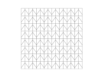
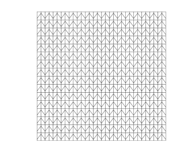
Figure 1: First computational mesh and first refined mesh in a sequence.

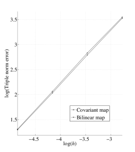
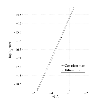
Figure 2: Error in triple norm and $L_{2}(\Omega)$ for $t=10^{-2}$.

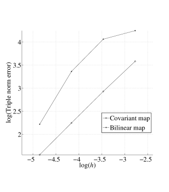
Figure 3: Error in triple norm and $L_{2}(\Omega)$ for $t=10^{-4}$.

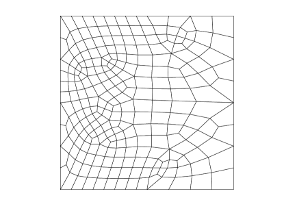
Figure 4: Mesh used to illustrate locking.

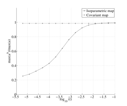
Figure 5: Locking using the isoparametric map.

References

- [1] D. N. Arnold, D. Boffi, and R. S. Falk. Approximation by quadrilateral finite elements. Math. Comp., 71(239):909–922, 2002.
- [2] D. N. Arnold, D. Boffi, and R. S. Falk. Remarks on quadrilateral Reissner–Mindlin plate elements. In H. A. Mang, F. G. Rammerstorfer, and J. Eberhardsteiner, editors, Fifth World Congress on Computational Mechanics, 2002.
- [3] D. N. Arnold, D. Boffi, and R. S. Falk. Quadrilateral finite elements. SIAM J. Numer. Anal., 42(6):2429–2451, 2005.
- [4] D. N. Arnold, F. Brezzi, R. S. Falk, and L. D. Marini. Locking-free Reissner-Mindlin elements without reduced integration. Comput. Methods Appl. Mech. Engrg., 196(37-40):3660–3671, 2007.
- [5] D. N. Arnold and R. S. Falk. A uniformly accurate finite element method for the Reissner-Mindlin plate. SIAM J. Numer. Anal., 26(6):1276–1290, 1989.
- [6] K. J. Bathe and E. N. Dvorkin. A four-node plate bending element based on Mindlin–Reissner plate theory and mixed interpolation. Int. J. Numer. Methods Engrg., 21:367–383, 1985.
- [7] L. Beirão da Veiga, A. Buffa, C. Lovadina, M. Martinelli, and G. Sangalli. An isogeometric method for the Reissner-Mindlin plate bending problem. Comput. Methods Appl. Mech. Engrg., 209–212:45–53, 2012.
- [8] P. R. Bösing, A. L. Madureira, and I. Mozolevski. A new interior penalty discontinuous Galerkin method for the Reissner-Mindlin model. Math. Models Methods Appl. Sci., 20(8):1343–1361, 2010.
- [9] S. C. Brenner, M. Neilan, and L.-Y. Sung. Isoparametric interior penalty methods for plate bending problems on smooth domains. Calcolo, 50(1):35–67, 2013.
- [10] D. Chapelle and R. Stenberg. An optimal low-order locking-free finite element method for Reissner-Mindlin plates. Math. Models Methods Appl. Sci., 8(3):407–430, 1998.
- [11] D. Chapelle and R. Stenberg. Locking-free mixed stabilized finite element methods for bending-dominated shells. In Plates and shells (Québec, QC, 1996), volume 21 of CRM Proc. Lecture Notes, pages 81–94. Amer. Math. Soc., Providence, RI, 1999.
- [12] D. Chapelle and R. Stenberg. Stabilized finite element formulations for shells in a bending dominated state. SIAM J. Numer. Anal., 36(1):32–73, 1999.
- [13] C. Chinosi and C. Lovadina. Numerical analysis of some mixed finite element method for Reissner-Mindlin plates. Comput. Mech., 16(1):36–44, 1995.
- [14] H.-Y. Duan and G.-P. Liang. A locking-free Reissner-Mindlin quadrilateral element. Math. Comp., 73(248):1655–1671, 2004.
- [15] R. G. Durán, E. Hernández, L. Hervella-Nieto, E. Liberman, and R. Rodríguez. Error estimates for low-order isoparametric quadrilateral finite elements for plates. SIAM J. Numer. Anal., 41(5):1751–1772, 2003.
- [16] G. Engel, K. Garikipati, T. J. R. Hughes, M. G. Larson, L. Mazzei, and R. L. Taylor. Continuous/discontinuous finite element approximations of fourth-order elliptic problems in structural and continuum mechanics with applications to thin beams and plates, and strain gradient elasticity. Comput. Methods Appl. Mech. Engrg., 191(34):3669–3750, 2002.
- [17] R. S. Falk, P. Gatto, and P. Monk. Hexahedral and finite elements. ESAIM Math. Model. Numer. Anal., 45(1):115–143, 2011.
- [18] P. Hansbo, D. Heintz, and M. G. Larson. A finite element method with discontinuous rotations for the Mindlin-Reissner plate model. Comput. Methods Appl. Mech. Engrg., 200(5-8):638–648, 2011.
- [19] P. Hansbo and M. G. Larson. A discontinuous Galerkin method for the plate equation. Calcolo, 39(1):41–59, 2002.
- [20] P. Hansbo and M. G. Larson. A -continuous, -discontinuous finite element method for the Mindlin-Reissner plate model. In Numerical mathematics and advanced applications, pages 765–774. Springer Italia, Milan, 2003.
- [21] P. Ming and Z.-C. Shi. Two nonconforming quadrilateral elements for the Reissner-Mindlin plate. Math. Models Methods Appl. Sci., 15(10):1503–1517, 2005.
- [22] X. Ye. A rectangular element for the Reissner-Mindlin plate. Numer. Methods Partial Differential Equations, 16(2):184–193, 2000.