Particle-in-cell simulations of collisionless shock formation via head-on merging of two laboratory supersonic plasma jets

Abstract

We describe numerical simulations, using the particle-in-cell (PIC) and hybrid-PIC code Lsp [T. P. Hughes et al., Phys. Rev. ST Accel. Beams 2, 110401 (1999)], of the head-on merging of two laboratory supersonic plasma jets. The goals of these experiments are to form and study astrophysically relevant collisionless shocks in the laboratory. Using the plasma jet initial conditions (density $\sim 10^{14}$–$10^{16}$ cm^-3, temperature $\sim$ few eV, and propagation speed $\sim 20$–100 km/s), large-scale simulations of jet propagation demonstrate that interactions between the two jets are essentially collisionless at the merge region. In highly resolved one- and two-dimensional simulations, we show that collisionless shocks are generated by the merging jets when immersed in applied magnetic fields ($B\sim 0.1$–1 kG). At expected plasma jet speeds of up to 100 km/s, our simulations do not give rise to unmagnetized collisionless shocks, which require much higher velocities. The orientation of the magnetic field and the axial and transverse density gradients of the jets have a strong effect on the nature of the interaction. We compare some of our simulation results with those of previously published PIC simulation studies of collisionless shock formation.

I Introduction

Collisionless shocks Sagdeev (1966); Sagdeev and Kennel (1991) play an important role in energy transport and evolution of charged-particle distribution functions in space and astrophysical environments. Although collisionless shocks in plasmas were first predicted in the 1950s Sagdeev (1966) and discovered in the 1960s Ness et al. (1964), many questions relating to the microscopic physics of collisionless shock formation, evolution, and shock acceleration of particles to very high energies remain unanswered pla ; wop . Laboratory studies of collisionless shocks have been conducted since the 1960s Podgornyi and Sagdeev (1969); Zakharov (2003), but a recent renaissance of laboratory collisionless shock experiments Woolsey et al. (2001); Horton et al. (2007); Ponomarenko et al. (2008); Romagnani et al. (2008); Constantin et al. (2009); Kuramitsu et al. (2011); Ross et al. (2012); Schaeffer et al. (2012); Swadling et al. (2013) stems from the fact that modern laboratory plasmas can satisfy key physics criteria for the shocks to have “cosmic relevance” Drake (2000). Recently initiated experiments Moser et al. (2012) at Los Alamos National Laboratory (LANL) aim to form and study astrophysically relevant collisionless shocks via the head-on merging of two supersonic plasma jets, each with order 10-cm spatial scale size. Compared to most other modern collisionless shock experiments which use laser-produced or wire-array Z-pinch Swadling et al. (2013) plasmas, the LANL experiment has larger shock spatial size (up to 30-cm wide and a few-cm thick) and longer shock time duration (order 10 $\mu$s) but somewhat lower sonic and Alfvén Mach numbers. The LANL experiment plans to have the capability to apply magnetic fields of a few kG (via coils) that can be oriented either parallel or perpendicular to the direction of shock propagation. Obtaining physical insights into and experimental data on collisionless shock structure, evolution, and their effects on particle dynamics are the primary reasons to conduct laboratory experiments on collisionless shocks. This paper reports results from particle-in-cell (PIC) and hybrid-PIC numerical simulations, using the Lsp code lsp ; Hughes et al. (1999), that informed the design of the LANL experiment and showed that collisionless shocks should appear with the expected plasma jet parameters.

After a brief description of the LANL collisionless shock experiment, the remainder of the paper describes single-jet propagation and one- (1D) and two-dimensional (2D) PIC head-on merging jet simulations. Our 1D magnetized simulations, in which the jets are immersed in an applied magnetic field, are similar to those of Shimada and Hoshino Shimada and Hoshino (2000) who performed 1D PIC simulations of magnetized shock formation using a reduced ion-to-electron mass ratio and a reflection boundary to model counter-propagating plasmas. We use the actual hydrogen mass ratio and the actual hydrogen plasma parameters expected in the LANL experiments, and we directly simulate both jets. This gives us the flexibility to independently vary the properties (e.g., the density profile) of the two jets without assuming any symmetry. We have also performed 2D Cartesian merging simulations of magnetized jets which allows us to consider the effects of the orientation of the magnetic field and plasma density gradients with respect to the jet propagation direction. These simulations demonstrate shock formation caused by the merging of magnetized jets with Mach numbers as low as $\approx 1.5$, where the Mach number is defined as Tidman and Krall (1971)

$$M=\frac{v_{1}}{v_{A}\sqrt{2(1+5\beta/6)}},$$ (1)

where $v_{1}$ is the pre-shock jet velocity in the shock frame, $v_{A}=B/\sqrt{2\mu_{o}n_{i}m_{i}}$ is the Alfvén velocity (in SI units) where $B$ is the pre-shock magnetic field strength $B$, $n_{i}$ is the pre-shock ion density, $m_{i}\gg m_{e}$ is the ion mass, and

$$\beta=\frac{T_{e}+T_{i}}{m_{i}v_{A}^{2}},$$ (2)

where the $T_{e}$ and $T_{i}$ are the pre-shock electron and ion temperatures in energy units.

In unmagnetized plasmas, collisionless shocks may also be formed by the Weibel instability Weibel (1959). Simulations of this mechanism were described by Kato and Takabe Kato and Takabe (2008), whose simulations were also performed at a reduced mass ratio and were restricted to relatively high velocities ($>0.1c$). When using the hydrogen mass ratio and a lower velocity ($\sim 100$ km/s as expected in the experiment), we find no shock formation on relevant timescales (a few $\mu$s).

The outline of the paper is as follows. In Sec. II we describe the simulation setup and numerical models used. In Sec. III, we present Lsp simulation results of single hydrogen jet propagation (Sec. III.1 and III.2) and 1D (Sec. III.3) and 2D (Sec. III.4) jet-merging with applied magnetic fields. Conclusions are given in Sec. IV.

II Numerical models and simulation setup

The simulations described in this paper are based on the LANL collisionless shock experiment Moser et al. (2012), which uses counter-propagating plasma jets formed and launched by plasma railguns Witherspoon et al. (2011); Thoma et al. (2011) mounted on opposite sides of a 2.74 m diameter spherical vacuum chamber (Fig. 1). Hydrogen, helium, and argon jets have been used in the experiments, but we focus exclusively on hydrogen in this paper due to its ability to better satisfy the physics criteria for cosmically relevant collisionless shocks Drake (2000). Single-jet parameters and evolution have been characterized experimentally Hsu et al. (2012a) in preparation for using an array of thirty such jets to form spherically imploding plasma liners as a standoff compression driver for magneto-inertial fusion Hsu et al. (2012b). For these collisionless shock studies, lower-density ($10^{14}$–$10^{16}$ cm^-3) and higher-velocity (100 km/s) jets are desired; this is accomplished primarily by reducing the injected mass for a given gun current.

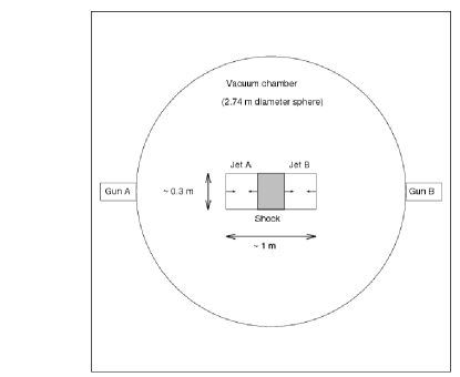
Figure 1: Schematic view of the experimental setup that is simulated in this paper.

The approach used in this numerical study is two-fold. We initially perform a large-scale simulation of a single jet propagating from the end of the plasma gun to the center of the vacuum chamber. The hydrogen jets emerge from the plasma gun with densities on the order of $10^{14}$–$10^{16}$ cm^-3 and temperatures of a few eV. The jets emerging from the guns will be few centimeters in size (on the order of the railgun aperture) with masses of a few $\mu$g, and will have a drift velocity $\sim 100$ km/s. But both must propagate on the order of 1 m before merging can begin, during which time the density, temperature, and equation-of-state (EOS) of the jet can change. The single-jet propagation simulation models the time evolution of the initial jet as it propagates through the chamber. This 2D $r$–$z$ simulation must be run for several $\mu$s. This requires using a fairly large timestep, for which $\omega_{pe}\Delta t\gg 1$ at an initial plasma density $\sim 10^{16}$ cm^-3, where $\omega_{pe}$ is the electron plasma frequency. Such simulations must be done with a hybrid-PIC approach in which electron plasma oscillations do need not to be resolved.

However, a fully kinetic approach is required to model the formation of shocks due to micro-instabilities induced by jet merging. As will be seen in Sec. III.1, the hydrogen jets ejected from the plasma guns drop considerably in density as they propagate to the center of the chamber where the merging takes place. This density reduction during propagation allows us to perform fully kinetic explicit PIC merging simulations in 1D and 2D Cartesian coordinates, in which electron timescales are resolved ($\omega_{pe}\Delta t<1$). So these simulations, which are initialized with plasma parameters obtained from the propagation simulation, are intended to model only the merging process which occurs much later than the ejection of the jets from the guns.

All of these simulations are performed using the hybrid-PIC code Lsp Hughes et al. (1999), which has been utilized widely and validated for applications in many areas of beam and plasma physics, including streaming instabilities Genoni et al. (2004); Rose et al. (2007) and Landau damping Rose et al. (2005). In addition to the traditional PIC paradigm, i.e., a Maxwell-Vlasov solver for collisionless plasmas in which electron length and time scales must be resolved, Lsp also contains algorithms for dense plasma simulation and includes physics modules for collisions (among charged and neutral species), EOS modeling, and radiation transport. This flexibility available in the code makes it useful for the two-fold simulation approach described above. All of the simulation results presented later in the paper have been checked to assure convergence of the relevant physics results with respect to numerical parameters such as cell size, timestep, and particle number per cell. To more fully focus on the physics results in the remaining sections of the paper, we provide in this section details on the models and numerical parameters used for the simulations.

II.1 Setup of hybrid single jet propagation simulation

The jet propagation simulation is performed in Lsp using a quasi-neutral hybrid-PIC algorithm Welch et al. (2011) which has fewer constraints on the timestep. The ion macroparticles are kinetic. But there are no electron macroparticles, as the ions carry fluid information for the inertia-less electrons. The equation of motion for the composite ion-electron macroparticle is given by

$$m_{i}n_{i}\frac{D}{Dt}\vec{v}=\vec{J}\times\vec{B}-\nabla P_{e}$$ (3)

where $\vec{v}$ is the macroparticle velocity, $P_{e}$ is the electron pressure, and $D/Dt$ is the full time derivative for the Lagrangian macroparticle. The current is given by Ohm’s law:

$$\vec{J}=\sigma\left(\vec{E}+\vec{v}^{*}\times\vec{B}+\frac{\nabla P_{e}}{en_{e}}\right)$$ (4)

where $n_{e}$ is the electron density, $\sigma$ is the conductivity, and $\vec{v}^{*}$ is the drift velocity gathered at the grid nodes. The fields, current, densities, and electron pressure gradient are all calculated at the nodes and then interpolated to the macroparticle position when Eq. (3) is applied. The full Maxwell’s equations are solved with the Ohm’s law term included. Displacement current is not dropped. Kinetic ions also undergo self-collisions (ion-ion). It is for this reason that there is no ion pressure contribution to Eq. (3). Coulomb collisions between electrons and ions species are included self-consistently through the Spitzer conductivity in Eq. (4). Particle energies are advanced by the same method which is described in Ref. Thoma et al. (2011). The plasma EOS (plasma internal energy, charge state, $\overline{Z}=n_{e}/n_{i}$, etc.) and opacity tables for radiation transport are provided by the Propaceos code MacFarlane et al. (2007). Although Lsp includes a full radiation transport algorithm Thoma et al. (2011), in this simulation we include only photon emission and neglect absorption. This allows radiation to be modeled as a simple energy sink on the fluid electron species. This approximation is justified in the optically thin regime, which is well satisfied for jets in the parameter regime under consideration.

The single jet propagation simulation is carried out in 2D $r$–$z$ cylindrical coordinates, as the jet is assumed to be azimuthally symmetric. This allows for full spatial hydrodynamic expansion of the jet in a 2D simulation. The simulation space is large enough to allow for propagation of the initial jet from the exit of the gun to the center of the vacuum chamber, and is bounded by perfectly conducting metal walls. The cell size is $\Delta r=\Delta z=0.5$ cm, and the timestep is given by $c\Delta t=32$ cm. The use of the uniformly stable exact-implicit field solver allows the simulation to be run with $c\Delta t\gg$ the cell size Zheng et al. (2000); Zheng and Chen (2001). The initial plasma is characterized by $\sim 1000$ ion macroparticles per cell. The results of the simulation are discussed in Sec. III.1.

II.2 Setup of fully kinetic 1D jet propagation and merging simulations

The 1D Cartesian fully kinetic propagation and merging simulations are initialized with input parameters based on results of the hybrid-PIC single jet propagation simulation. As will be seen in Sec. III.1, the jets at the chamber center have a much lower density ($\sim 10^{13}$ cm^-3) than when ejected from the plasma guns. This allows us do explicit kinetic PIC simulations. We can also afford better spatial and temporal resolution in 1D Cartesian coordinates: $\Delta x=2c\Delta t=0.03$ cm. Since the timestep is small, an explicit field solution is used rather than the exact-implicit solver. Both electrons and ions are modeled kinetically. Coulomb collisions are included for the electron species, as are ion collisions, which are found to have a negligible effect in this parameter regime. The cell size and time step given above resolve not only $\omega_{pe}$, but also the ion and electron cyclotron frequencies ($\omega_{ci}$ and $\omega_{ce}$, respectively), and ion and electron skin depths ($d_{i}\equiv c/\omega_{pi}$ and $d_{e}\equiv c/\omega_{pe}$, respectively). A cloud-in-cell Birdsall and Langdon (1991) particle model allows $\Delta x>$ the Debye length. The 1D simulations described below are all run with several thousand macroparticles per cell. We assume fully stripped hydrogen ions ($\overline{Z}=1$) for simplicity. Some justification for this assumption is given below. We also assume an ideal gas EOS for the plasma jets and neglect radiation losses.

We initially perform a few fully kinetic single-jet propagation simulations with and without magnetic fields to demonstrate the effect of applied fields on single jet propagation. These results are described in Sec. III.2. In Sec. III.3 we discuss the results of 1D fully kinetic simulations of two-jet merging with and without applied magnetic fields. We consider the effects of varying magnetic field strengths, as well as the effect of finite density gradients (with scale length $L_{d}$), and the effect of the initial spatial separation, or gap $L_{g}(0)$, between the two jets.

II.3 Setup of fully kinetic 2D jet merging simulations

The last group of simulations considered in this paper are in 2D Cartesian coordinates. We simulate the 2D jets in the $x$–$y$ plane, with the jets propagating in the $x$ direction. The total $y$ extent is many $d_{i}$ wide, and periodic boundaries are imposed at minimum and maximum values of $y$. To maintain reasonable runtimes, 2D simulations performed at realistic length scales (jet lengths $L_{j}\sim 10$–100 cm) require coarser spatial resolution ($\Delta x=\Delta y=2c\Delta t=0.24$ cm) and a smaller number of particles per cell (tens rather than hundreds) than were possible in 1D. Coulomb collisions are included, but we again assume an ideal EOS and neglect radiation transport (both photon emission and absorption).

In Sec. III.4 we consider the results of 2D Cartesian simulations of counter-propagating jets in perpendicular magnetic fields. As in 1D, the jet propagation remains in the $x$ direction, and we simulate the 2D jets in the $x$–$y$ plane. The total $y$ extent is many $d_{i}$ wide, and periodic boundaries are imposed at minimum and maximum values of $y$.

In these simulations we find some slow numerical heating of the electrons at later times due to the coarse spatial resolution of the grid ($\Delta x\sim c/\omega_{pe}$). However, if the simulation duration does not exceed $\sim 1$ $\mu$s, the energy conservation remains good to within a few percent. High fidelity simulations over longer time scales will require better spatial resolution and larger particle numbers. This will require the use of more processors than were available.

III Simulation results

III.1 Hybrid-PIC simulation of single hydrogen plasma jet propagation

Hybrid-PIC Lsp simulations were performed of a single hydrogen plasma jet propagating from the railgun nozzle to the center of the chamber in order to connect the plasma jet parameters at the railgun exit with those in the region of head-on jet merging. Details on the simulation setup and numerical methods are given in Sec. II.1. The initial ion density $n_{i}$ profile can be in seen in the upper left plot in Fig. 2. At $t=0$ the single jet is assumed to have a peak density $n_{i}(t=0)=10^{16}$ cm^-3 (total mass $\sim 10$ $\mu$g), electron and ion temperatures $T_{e}(0)=T_{i}(0)=5$ eV, and $v_{j}=150$ km/s (in the $-z$ direction). The initial jet parameters are also given in Table 1.

The time evolution of the jet propagation can be seen in Fig. 2, which shows $n_{i}$ contours at $t=0$, $3.8$, $5.4$, and $7$ $\mu$s. Figure 3 shows $n_{i}$ line-outs at the same times. The approximate plasma parameters of the jet at the center of the chamber ($z=0$ cm) are also given in Table 1. So this simulation determines the approximate parameter regime of the individual jets after they have propagated to the center of the chamber and begun to merge: $n_{i}\simeq 10^{13}$ cm^-3, $v_{j}\simeq 150$ km/s, $T_{e}\simeq T_{i}\simeq 1$ eV, $\overline{Z}=n_{e}/n_{i}\sim$ 1, and $L_{j}\sim 50$ cm. We note that from spectroscopic data obtained from the LANL experiment the plasma density at the chamber center can be inferred to be below $10^{14}$ cm^-3, which is consistent with the simulation result. The experimental jets are expected to be somewhat colder when emerging from the guns than the 5-eV value used in the simulations. But in the simulation results radiation cooling quickly causes the jet temperature to drop. Nonetheless, we expect the amount of density decay seen in the simulation to be an upper bound on the experiments.

Based on the results of this simulation, we have chosen a set of simplified plasma parameters to be used for the fully kinetic simulations discussed in the following subsections. These values are given in Table 2. Using these parameters we can estimate the Coulomb collision frequency for the jets. To observe collisionless merging of the jets, it is necessary that the inter-jet ion collision time be much larger than the jet interaction time $L_{j}/v_{j}$. For two counter-propagating ion beams ($v_{j}\gg v_{th,i}$, the ion thermal velocity), the Spitzer collision frequency is proportional to $|2v_{j}|^{-3}$ Rambo and Procassini (1995). Using the parameters above, we find $\nu_{ii}^{-1}\sim 10^{-4}$ s. The ion stopping time due to collisions with electrons in the opposing jet is $\nu_{ie}^{-1}\sim 10^{-5}$ s, while the jet interaction time $L_{j}/v_{j}\sim 10^{-6}$ s. So this simulation result demonstrates that these counter-propagating jets will indeed be in the collisionless regime when the jets merge at the center of the chamber, allowing the LANL facility to be used for the investigation of collisionless shock formation.

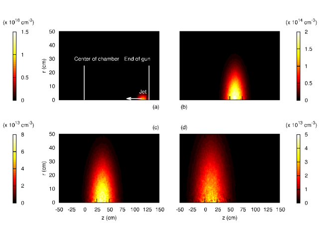
Figure 2: Snapshots of ion density in a 2D $r$–$z$ hybrid-PIC simulation of hydrogen jet propagation from the end of the plasma gun to the center of the chamber. Initial jet parameters are given in Table 1. Densities are shown at $t=$ (a) 0, (b) 3800, (c) 5400, and (d) 7000 ns.

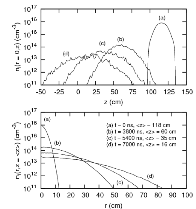
Figure 3: Line-outs of ion density in a 2D $r$–$z$ hybrid-PIC simulation of hydrogen jet propagation from the end of the plasma gun to the center of the chamber. Densities are shown at $t=$ (a) 0, (b) 3800, (c) 5400, and (d) 7000 ns. (Top) Line-outs vs. $z$ at $r=0$. (Bottom) Line-outs vs. $r$ at $z=\langle z(t)\rangle$, which is the instantaneous, longitudinal jet center-of-mass.

Table 1: Initial and approximate parameters at the center of the chamber ($z=0,t\simeq 8400$ ns) in 2D $r$–$z$ jet propagation simulation (see also Figs. 2 and 3).

Quantity	Railgun Exit	Chamber Center
$n_{e}$ (cm-3)	$10^{16}$	$9\times 10^{12}$
$n_{i}$ (cm-3)	$10^{16}$	$2\times 10^{13}$
$T_{e}$ (eV)	$5$	$1.25$
$T_{i}$ (eV)	$5$	$0.4$
$v_{j}$ (km/s)	$150$	$150$

Table 2: Initial jet parameters used in 1D and 2D fully kinetic propagation and merging simulations. For simulations with density gradients, the density value refers to the peak value. Magnetic field values refer to the unperturbed applied field strength

Quantity	Value
$n_{i}=n_{e}$ (cm-3)	$10^{13}$
$T_{i}=T_{e}$ (eV)	1
$v_{j}$ (km/s)	150
$L_{j}$ (cm)	$\sim 50$
$L_{d}$ (cm)	varies: $\sim[0,L_{j}]$
$B$ (G)	varies: $\sim[0,1500]$
$\nu_{ii}^{-1}$ (s)	$\sim 10^{-4}$
$\nu_{ie}^{-1}$ (s)	$\sim 10^{-5}$
$L_{j}/v_{j}$ (s)	$\sim 10^{-6}$

III.2 Fully kinetic single-jet simulations in 1D

We now consider fully kinetic, highly resolved 1D Cartesian simulations of jet propagation in the merge region, with and without an applied perpendicular magnetic field. The initial jet has a uniform density of $n=10^{13}$ cm^-3. The scale lengths of the initial gradients at the edges of the jet are on the order of a cell width. This simplified density profile is used to illustrate more clearly the effect of the magnetic field on single-jet propagation. Such a flat-top profile also allows for very clear shock structure to develop in the two-jet simulations discussed in Sec. III.3. The full set of initial conditions are given in Table 2. Although we imposed the initial condition $\overline{Z}=1$, there is no noticeable charge separation between the kinetic electron and ion species as the simulation advances, i.e., quasi-neutrality ($n_{e}\simeq n_{i}$) holds throughout. The jet propagates in the $+x$ direction, with $x=0$ (chamber center) representing the merge point. Although there is no second jet in the simulations in this subsection, we stress this choice of origin now, as it is retained throughout the rest of the paper. The initial $n_{i}$ profile and ion macroparticle $x$–$v_{x}$ phase-space distribution are shown in Fig. 4(a). Each red dot in the phase-space plots ($v_{x}$ is plotted on the right axis) represents an ion macroparticle, each of which has the same charge weight.

Figure 4(b) shows the $n_{i}$ profile and ion velocity distribution at $t=1500$ ns with no applied magnetic field. The spreading of the $n_{i}$ profile in time at the jet edges is due to ambipolar diffusion. Due to the initial density profile, the peak density does not drop because sound waves have not had time to propagate fully into the jet. The addition of an applied transverse magnetic field of $1$ kG suppresses the spreading of the density profile [Fig. 4(c)], explained as follows. There is a motional electric field $E_{y}$ embedded in the bulk of the jet which allows $\vec{E}\times\vec{B}$ drifting of the jet at $\vec{v}_{j}$ through the magnetic field aligned in the $+z$ direction. But electrons which stray from the bulk are line-tied, restricting ambipolar diffusion. The $E_{y}$, with the appropriate magnitude of $v_{j}B$, can be clearly observed in the simulation results.

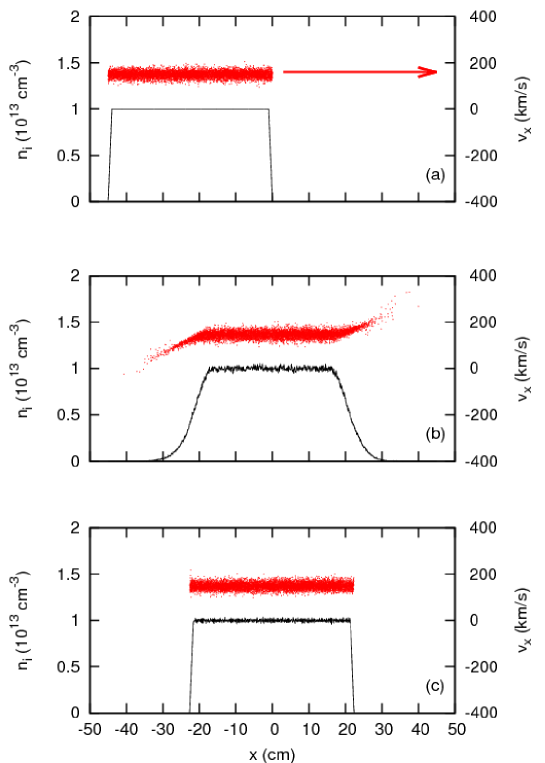
Figure 4: Fully kinetic, 1D, single-jet propagation simulation results for ion density $n_{i}$ and ion macroparticle $x$–$v_{x}$ phase-space data versus $x$ at (a) $t=0$, and at $t=1500$ ns with (b) no applied magnetic field and (c) $B_{z}=1$ kG.

III.3 Unmagnetized and magnetized jet merging in 1D

We now consider merging of two counter-propagating jets to look for evidence of shock generation, and two possible collisionless shock mechanisms. The first is a Weibel-mediated unmagnetized shock driven by a 2D electromagnetic kinetic instability when the two jets merge Kato and Takabe (2008). In 2D PIC simulations, Kato et al. Kato and Takabe (2008) found unmagnetized Weibel-mediated shocks for merging jets with “non-relativistic” velocities $v_{j}=(0.1$–$0.45)c$. Using Lsp in similar simulations, we are able to reproduce the results of Kato for collisionless merging jets with velocities in this velocity range. But $0.1c$ is still 200 times faster than the 150 km/s jet velocities expected in the LANL experiments. When scaling the Weibel simulations down to the experimental parameter regime (and using the actual hydrogen mass ratio $m_{i}/m_{e}=1836$), we find no evidence of shock formation or any strong jet interaction over $\mu$s time scales, suggesting that the LANL experiment will not give rise to unmagnetized collisionless shocks. The second possible mechanism is a magnetic shock which occurs when jets merge while immersed in perpendicular magnetic fields ($\vec{B}\cdot\vec{v}_{j}=0$) Kato and Takabe (2008); Tidman and Krall (1971). For the remainder of the paper, we consider 1D and 2D simulation results for merging jets in such applied magnetic fields.

The 1D merging simulations are initiated with the jets near the merge point, after which they are allowed to collide. Our simulations are similar to those of Shimada and Hoshino Shimada and Hoshino (2000), but we explicitly model both jets (rather than the reflecting particle boundary used by Shimada et al.). This allows us to incorporate arbitrary density profiles for each jet. Again, we use the real value of $m_{i}/m_{e}$ for the hydrogen jets rather than a reduced mass ratio. Details on the simulation setup were given in Sec. II.2.

III.3.1 Unmagnetized jet merging

We now consider two counter-propagating jets in the absence of an applied field. This situation in shown in Fig. 5, which shows $n_{i}$ and particle $x$–$v_{x}$ phase-space data as a function of $x$ at various times. There is relatively little interaction between jets in the absence of an applied magnetic field. There are two distinct ion populations in the phase-space plot representing each of the two jets, and the density doubles where the two jets interpenetrate. This behavior demonstrates that ions are effectively collisionless in this parameter regime (recall that Coulomb collisions are fully included in the simulation and their effect, if significant, would be visible in the ion phase-space). This is consistent with the estimates given for the jet interaction time and ion collision times in Table 2. We also note that since this is a 1D simulation, there is no possibility here of observing the Weibel-driven shock, which requires at least 2D modeling.

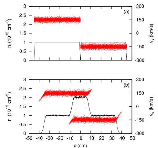
Figure 5: Simulation (1D) results for two counter-propagating jets without an applied magnetic field. Initial jet parameters are given in Table 2. Ion densities and particle $x$–$v_{x}$ phase-space data are shown as a function of $x$ at (a) $t=0$ and (b) $t=1500$ ns.

III.3.2 Magnetized jet merging

We now repeat the two jet simulation from Sec. III.3.1 but add an applied magnetic field, $B_{z}=1000$ G. Results from this simulation are shown in Fig. 6. In this case there is clear propagation of a shock wave. There is a finite width shock transition region, with clear pre- and post-shocked regions with roughly constant density and field values for each region. The persistence of the density null at $x=0$ can be explained as follows. Each jet travels in a motional field $E_{y}\sim v_{x}B_{z}$, which has opposite signs for the two jets ($v_{x}=\pm v_{j}$). At the merge point, $x=0$, the motional fields cancel and the plasma can no longer propagate in the magnetic field. Alternately, the enhanced magnetic field in the shocked region is supported by plasma currents at the shock edge. The $\vec{J}\times\vec{B}$ force decelerates the plasma from a drift velocity of $v_{j}$ in the pre-shocked region to zero in the post-shocked region. This can be seen in the phase-space plots. Since the plasma is stationary behind the shock, the density profile remains relatively constant in time. At early times, as the jets begin to merge, the electric field $E_{x}$, which establishes the current flow, can be seen in the simulation results. This field also causes the acceleration of a small population of ions near $x=0$ cm, which can be seen in Fig. 6.

We now briefly discuss the electron behavior. We have already mentioned that quasi-neutrality is maintained throughout all of the simulations. There is no noticeable charge separation on length scales greater than a cell width. But the electron velocity distribution does not exhibit the clear structure which is observed in the ion phase-space plots. There is only a sharp discontinuity in the electron velocity spread (temperature) at the shock edge. Any more detailed shock structure in the electron phase-space data is obscured by the thermal spread of the electrons in the simulations. For this reason we present only the ion phase-space data. We also note that we did not observe strong electron acceleration on $\mu$s time scales, as seen by Shimada et al. in their scaled simulations.

We have demonstrated the development of a propagating shock wave in simulations with a perpendicular magnetic field. We find no interaction between the jets if a parallel magnetic field is applied. There is also no interaction for small values of perpendicular magnetic field, i.e., when $v_{A}\ll v_{j}$.

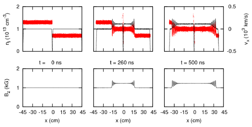
Figure 6: Simulation (1D) results for two counter-propagating jets with an applied perpendicular field (in $+z$ direction) of $1$ kG. Initial jet parameters are given in Table 2. Ion density, $B_{z}$, and ion macroparticle $x$–$v_{x}$ phase-space data are shown as a function of $x$ at (left column) $t=0$, (middle column) $t=260$ ns, and (right column) $t=500$ ns.

III.3.3 Effect of varying magnetic field magnitude

We now consider the effect of varying the field magnitude. In Fig. 7 we show results from a series of simulations with varying values of applied field. The shock wave is evident at all these field strengths, but other kinetic ion effects are also visible. The ripples in the density and field profiles in the shock transition region ($|x|\sim[10,15]$ cm) have a spatial period $\propto B$ (pre-shock field magnitude), and the ripple amplitude grows with time. The shock transition region width is approximately equal to $d_{i}$ and is roughly independent of $B$ and $t$. But simulations with longer jets are required to conclusively show this scaling. An explanation for the ion acceleration mechanism at the initial merge point, $x\sim 0$, was explained above. Individual ions accelerated at the shock edge, $|x|\sim 15$ cm, spin around in phase-space with a period $\tau\propto 1/B$ (but $\ll 2\pi/\omega_{ci}$) and a spatial extent of order the ion Larmor radius $\sim r_{Li}\geq d_{i}$.

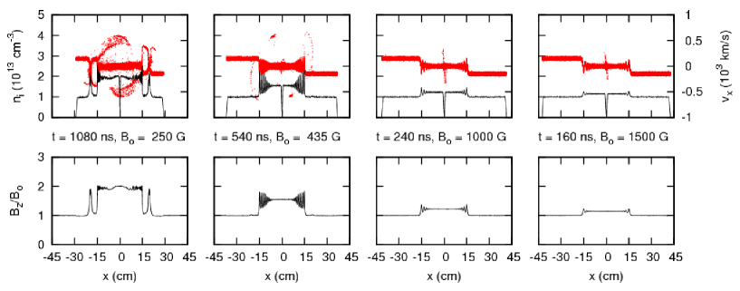
Figure 7: Simulation (1D) results for two counter-propagating jets with varying applied perpendicular fields strengths (with magnitude $B_{0}$ in the $+z$ direction). Initial jet parameters are given in Table 2. Ion density, $B_{z}$, and macroparticle $x$–$v_{x}$ phase-space data are shown as a function of $x$. All plots are shown with the shock edge roughly at the same position, $|x|\sim 15$ cm.

For these simple 1D simulations, it is possible to compare our results to the theoretical Rankine-Hugoniot conditions for collisionless shocks in perpendicular fields. First, we define the regions of the simulation space in Fig. 8. Region 1 is the pre-shocked unperturbed region, and region 2 is the post-shocked region, and we denote the transition region as “S.” In the simulation frame, the S region propagates to the right in Fig. 8 at a shock velocity denoted as $v_{s}$. The theoretical treatment given by Tidman and Krall Tidman and Krall (1971), however, considers the shock frame, i.e., the frame where the shock transition region is stationary. For a perpendicular magnetized shock, $\vec{B}$ is perpendicular to both $\vec{v_{1}}$ and $\vec{v_{2}}$, which are the pre- and post-shocked velocities (both in the $x$ direction), respectively, in the shock frame. Assuming Maxwellian distributions for ions and electrons, the Rankine-Hugoniot relations Tidman and Krall (1971) are given by

$$\frac{n_{1}}{n_{2}}=\frac{B_{1}}{B_{2}}=\frac{v_{2}}{v_{1}}=\frac{1}{8}\left(1+\frac{5B_{1}^{2}(1+\beta)}{2\mu_{o}m_{i}n_{1}v_{1}^{2}}+\left[1+\frac{5B_{1}^{2}(1+\beta)}{2\mu_{o}m_{i}n_{i}v_{1}^{2}}+\frac{8B_{1}^{2}}{\mu_{o}m_{i}n_{1}v_{1}^{2}}\right]^{1/2}\right),$$ (5)

and the Mach number of the shock is given by Eq. (1). We note that there is a typographical error in the Rankine-Hugoniot conditions in Ref. Tidman and Krall (1971), but in Eq. (5) the error has been corrected. Also, since the theory assumes thermal distributions for both electrons and ions, it does not account for any of the ion kinetic effects seen in Fig. 7. We note from Eq. (1) that in the limiting case where $\beta\ll 1$, $M$ is the Alfvén Mach number, $v_{1}/\sqrt{2}v_{A}$. In the opposite limit ($\beta\gg 1$), $M$ becomes the sonic Mach number.

From the simulation results, the velocity ratio in the shock frame is calculated by

$$v_{1}/v_{2}=(v_{j}+v_{s})/v_{s}.$$ (6)

The results for the density, magnetic field and velocity ratios, as well as the Mach number, are shown Table 3. We see that for all our merging simulations, we are in the low-$\beta$ regime. In the 1D simulations, we always find $n_{1}/n_{2}\simeq B_{2}/B_{1}\simeq v_{1}/v_{2}$. There is good agreement with the theoretical values from the Rankine-Hugoniot conditions, except at lower $B_{z}$ values which are strongly perturbed by ion acceleration from the shock edge [a kinetic effect not accounted for in Eq. (5)]. This gives us confidence that we can quantitatively describe shock phenomena using PIC methods.

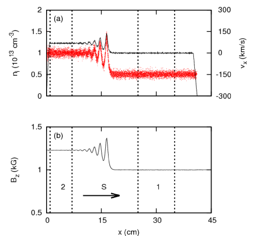
Figure 8: Simulation (1D) results for two counter-propagating jets with a $1$-kG perpendicular field in the $+z$ direction. Only the initially right-propagating jet is shown here. In the full simulation there is essentially mirror symmetry about $x=0$. Initial jet parameters are given in Table 2. (a) Ion density and particle $x$–$v_{x}$ phase-space data, and (b) $B_{z}$ are shown as a function of $x$ at $t=260$ ns, a time well after the establishment of the propagating shock.

Table 3: Comparison of 1D simulation results to the Rankine-Hugoniot conditions of Eq. (5). Initial jet parameters are given in Table 2

. $B_{1}(G)$ $\beta$ $n_{2}/n_{1}=B_{2}/B_{1}$ $v_{1}/v_{2}$ Theory $M$ $250$ $0.026$ 2.0 2.09 1.79 1.65 $350$ $0.013$ 1.7 1.69 1.63 1.51 $435$ $0.0085$ 1.55 1.52 1.55 1.45 $500$ $0.0064$ 1.48 1.44 1.48 1.41 $1000$ $0.0013$ 1.22 1.22 1.26 1.22 $1500$ $0.0008$ 1.15 1.15 1.19 1.15

III.3.4 Effects of realistic density gradient at and gap size between jet leading edges

The previous 1D shock simulations were performed with very steep density gradients (on the order of one or two cell widths), and a uniform density in the bulk. These profiles were chosen because they exhibited very clear shock structure and allowed direct comparison with the 1D theory. We now add more realistic density gradients. In the experiment we expect density profiles such as those seen at later times in Fig. 2, with $L_{d}\sim L_{j}$. The applied field is $B_{z}=1000$ G, and the maximum initial density remains $10^{13}$ cm^-3. The initial density profile can be seen at the top left of Fig. 9. The time evolution of the density, particle phase-space, and magnetic field are shown in the figure as well. We note that there is still a clear shock wave structure visible when finite density gradients are included. Due to the presence of initial density gradients, there are no constant post-shock values of $n_{2}$ and $B_{2}$, but the sharp shock transition region is evident.

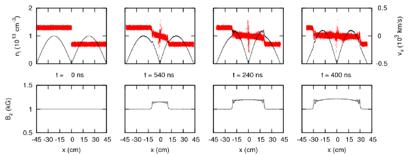
Figure 9: Simulation (1D) results for two counter-propagating jets with finite density gradients in an applied perpendicular magnetic field (1 kG in the $+z$ direction). Initial jet parameters are given in Table 2. Ion density, $B_{z}$, and particle $x$–$v_{x}$ phase-space data are shown as a function of $x$.

All the 1D shock simulations discussed above were initialized with two counter-propagating jets adjacent to each other (see the top left of Fig. 6). This was done essentially to minimize the run-time required to observe the interaction. We now wish to consider the effect of an initial jet separation. We repeat the simulation with constant bulk density and sharp density gradients and $B_{z}=350$ G (with shock parameters given in Table 3), but now introduce a large initial jet separation $L_{g}(0)\sim L_{j}$. The initial geometry is shown in Fig. 10, as well as the time evolution of ion density, ion particle phase-space, and magnetic field. The interaction seen in this figure is not a shock wave. At these early times there is no clear post-shocked region: $n_{2}$ and $B_{2}$ never reach constant steady-state values (despite the uniform initial density). Moreover, the disturbance propagates into the jet at a speed $\sim v_{A}$ (in the jet rest frame).

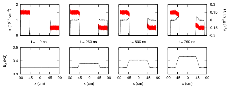
Figure 10: Simulation (1D) results for two counter-propagating jets with a $350$ G perpendicular field in the $+z$ direction and an initial jet separation of $\sim 90$ cm. (Top) Ion density and particle $x$–$v_{x}$ phase-space data, and (bottom) $B_{z}$ are shown as a function of $x$ at $t=0$, 260, 500 and 760 ns.

We now also repeat the simulation at 1000 G with a larger initial jet separation. Some results are shown in Fig. 11. At early times we again see the Alfvénic disturbance propagate into the jets. But later, at about 500 ns in this case, a shock wave begins to form, as evidenced by the sharp discontinuity in the magnetic field and the broad spread in ion velocities. Upstream of the shock, we notice deceleration of the ions in the Alfvénic propagation region. In a series of such simulations, we have noticed that the shock wave is initiated only when there is a significant population of ions with $v_{x}\sim 0$. The shock wave was not observed in the $350$ G simulation (Fig. 10) because it was not run long enough for any ions to be slowed to small enough values of $v_{x}$.

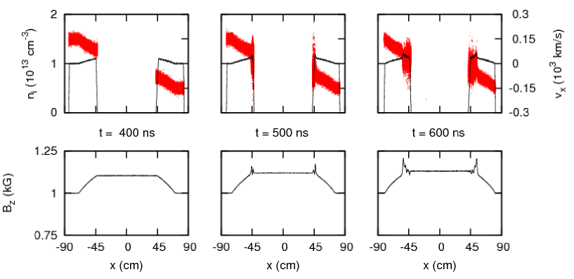
Figure 11: Simulation (1D) results for two counter-propagating jets with a $1$ kG perpendicular field in the $+z$ direction and an initial jet separation of $90$ cm. Ion density, particle $x-v_{x}$ phase-space data (top), and $B_{z}$ (bottom) are shown as a function of $x$ at $t=400$, $500$, and $600$ ns.

A simple model can be used to explain the early-time behavior (pre-shock) of the 1D counter-propagating jet simulations with an initial jet separation. To facilitate the discussion, we introduce some nomenclature in Fig. 12. The initial gap separation at at $t=0$ (top plot in figure) is $L_{g}(0)$, and the instantaneous gap separation $L_{g}(t)$ is shown in the middle plot, which shows the ion density after 800 ns. We also define the time-dependent magnetic field strength at the midpoint between the jets as $B_{m}(t)$.

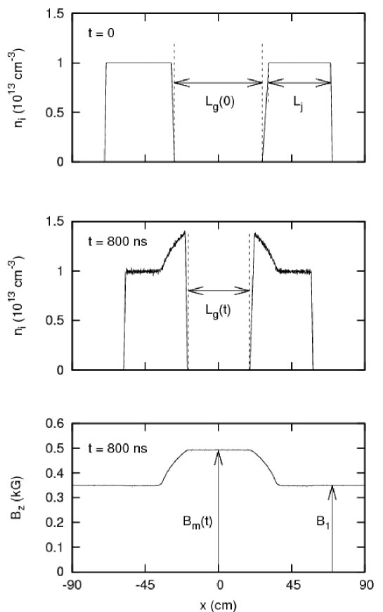
Figure 12: Two-jet simulation with an applied field of $350$ G and an initial jet separation of $\sim 45$ cm. The full initial conditions are given in Table 2. The ion density is shown at (top) $t=0$, and (middle) 800 ns. The magnetic field is also shown (bottom) at $t=800$ ns.

In all these simulations (before the onset of shock waves), we observe flux conservation, i.e.,

$$L_{g}(t)\times B_{m}(t)\sim\mbox{constant},$$ (7)

and a uniform acceleration of gap distance:

$$L_{g}(t)\sim L_{g}(0)-2v_{j}t+1/2at^{2},$$ (8)

where $a>0$ is a constant acceleration value. This can be seen explicitly in Fig. 13, which plots $\Delta L_{g}[=L_{g}(t)-L_{g}(0)]$ as a function of time for a simulation with $v_{j}=150$ km/s, $L_{g}(0)=94$ cm, $L_{j}=42$ cm, and $B_{1}=350$ G. We have also plotted $\Delta L_{g}$ as given by Eq. (8) with a constant acceleration of $a=12$ cm$/\mu$s², which was determined by least-squares fitting.

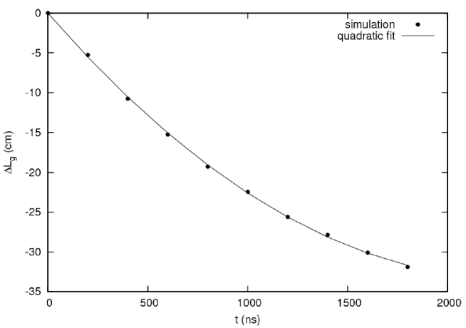
Figure 13: Change in jet separation distance $\Delta L_{g}$ as a function of time. The simulation data is compared to a quadratic fit based on Eq. (8).

To derive an estimate for the gap acceleration, we consider a simplified model of the 1D simulations. This is shown in Fig. 14. We neglect displacement current, assume linear ramps on $B_{z}$, and a piecewise constant current $J_{y}$. By imposing flux conservation and assuming a $\vec{J}\times\vec{B}$ force ($\beta\ll 1$) on the plasma in the transition region, we obtain

$$a=4v_{A}v_{j}/L_{g}(0),$$ (9)

where $v_{A}$ is calculated using the applied field $B_{1}$.

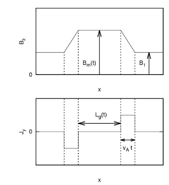
Figure 14: Schematic view of Alfvén wave propagation in merging jet simulations.

In Table 4 we list the acceleration measured in a series of simulations with varying values of $B_{1}$, $L_{g}(0)$, $L_{j}$, and $v_{j}$. According to the simple theory of Eq. (9) the normalized acceleration $aL_{g}(0)/v_{A}v_{j}$ should be equal to 4. The Lsp simulations are seen to be in relatively good agreement with the simple scaling derived above. If we define the minimum jet separation as $L_{min}$, our simple theory predicts that

$$L_{min}/L_{g}(0)=1-v_{j}/2v_{A}.$$ (10)

This implies that the jets will not overlap unless $v_{j}>2v_{A}$. But, as we see in Fig. 11, the shock waves start before $L_{g}$ can reach 0.

Table 4: Comparison of 1D simulation results to simple theory [Eq. (9)] of Alfvén wave propagation into jets with a large initial separation.

$B_{1}(G)$	$L_{g}(0)$ (cm)	$L_{j}$ (cm)	$v_{j}$ (km/s)	$aL_{g}(0)/v_{A}v_{j}$
$1000$	94	42	150	2.90
$350$	94	42	150	3.23
$350$	54	42	150	2.79
$350$	94	42	300	4.22
$350$	54	62	150	3.0

III.4 Unmagnetized and magnetized jet merging in 2D

In this section we consider the results of 2D Cartesian simulations of counter-propagating jets in perpendicular magnetic fields. The jet propagation remains in the $x$ direction, and we simulate the 2D jets in the $x$–$y$ plane. In 2D, we now have to explicitly specify the direction of the perpendicular field in the $y$–$z$ plane. Details on the simulation setup were given in Sec. II.3.

We consider initially a quasi-1D simulation with no variation of any physical quantity in the $y$ direction and periodic boundaries in $y$. The initial density profiles can be seen in the top row of Fig. 15. The full initial conditions for all the 2D runs are given in Table 2. The total $y$ extent is many $d_{i}$ wide. The initial conditions are $n_{1}=10^{13}$ cm^-3, $T_{e1}=T_{i1}=1$ eV. The magnetic field is in the $+z$ direction ( analogous to the 1D simulations as the field is aligned in a virtual direction) with $B_{1}=350$ G and $v_{j}=150$ km/s.

We first note from the bottom row of Fig. 15, which shows $n_{i}$ and $B_{z}$ contours at $t=800$ ns, well after the shock formation, that there is no strongly evident structure in the $y$ direction in the bulk of the jets, although the $y$ extent is many $d_{i}$ wide. There is some small density variation along the $x=0$ line where the density is very low, but these variations are on the order of a cell size and are probably due to particle noise.

Due to the coarse spatial grid, we can no longer resolve the oscillatory structure along the $x$-direction in the shock transition region, which were seen in the highly resolved 1D simulations (e.g., see Fig. 6). But we obtain the same shock speed (i.e., $M$) and density discontinuity, $n_{2}/n_{1}(=B_{2}/B_{1}=v_{1}/v_{2})$, as the corresponding 1D simulation.

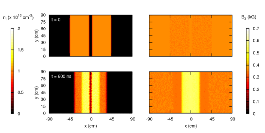
Figure 15: Results from 2D jet merging simulations. Initial jet parameters are given in Table 2. The left column shows ion density contours and the right magnetic field strength $B_{z}$ at (top row) $t=0$ and (bottom row) $t=800$ ns, well after shock formation.

We now consider two uniform density disks with no applied magnetic field. The periodic boundaries in $y$ have been retained. Ion density contours and $x$–$v_{x}$ particle phase-space data are shown in Fig. 16. The results are analogous to the unmagnetized 1D case, i.e., there is very little interaction between the jets in this parameter regime in the absence of an applied magnetic field. There is certainly no evidence of Weibel-induced unmagnetized shock waves on time scales $\sim 1$ $\mu$s.

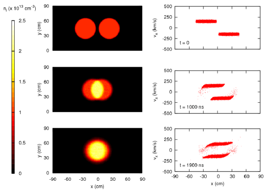
Figure 16: Simulation (2D) of two counter-propagating plasma jets in the absence of a magnetic field. Ion density contours and ion $x$–$v_{x}$ phase-space data are shown at various times. There is essentially no interaction between the two jets.

We repeat the previous simulation but now add a 350-G magnetic field in the virtual direction ($+z$). The $n_{i}$ and $B_{z}$ contours are shown at various times in Fig. 17. Along the line $y=45$ cm, we find approximate values of $n_{2}/n_{1}\sim B_{2}/B_{1}\sim 1.5$, and $v_{1x}/v_{2x}\sim 2.4$, and a shock velocity of $v_{s}\sim 210$ km/s. Although the problem is now inherently 2D, we nonetheless estimate $M\sim 1.4$ from the 1D formula of Eq. (1).

We notice, however, that there is a conspicuous difference between this simulation and the 1D and quasi-1D (Fig. 15) analogs. Namely, the density at the center-of-mass of the two jets, along the line at $x=0$, remains large ($\geq 10^{13}$ cm^-3) throughout the simulation, indicating at least some jet interpenetration at this point. In the 1D analogs, the density remained close to zero at the jet center of mass.

In order to explain this qualitatively different behavior, we consider first the results for a 2D simulation in which the 350-G field is rotated from the virtual $+z$ to the $+y$ direction, which lies in the simulation plane. These results are shown in Fig. 18. For this simulation we find, along $y=45$ cm, that $n_{2}/n_{1}\sim B_{2}/B_{1}\sim v_{1}/v_{2}\sim 1.5$ and $M\sim 1.6$. For this magnetic field orientation, the results are qualitatively similar to the 1D case, as $n_{i}$ remains zero along $x=0$.

When the magnetic field is in the $y$ direction (Fig. 18), the currents which drive the magnetic field, $B_{2}>B_{1}$, can flow in the virtual $z$ direction and remain localized near $x=0$ cm. This allows for large $\vec{J}\times\vec{B}$ forces to reflect the incoming the jets. When the magnetic field is in the virtual $z$-direction (Fig. 17) the magnetic field is supported by finite circular current paths around the perimeter of the bulk of the jet. The density gradient in $y$ acts to minimize the $x$ component of the $\vec{J}\times\vec{B}$ force on the jets.

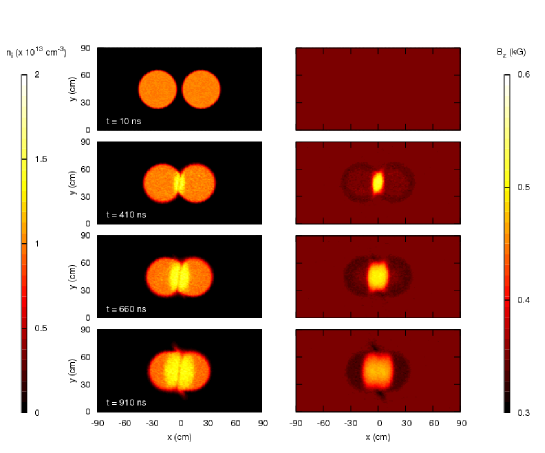
Figure 17: Simulation (2D) of two counter-propagating plasma jets with a 350-G magnetic field in the $+z$ direction. Ion density and $B_{z}$ contours are shown at various times.

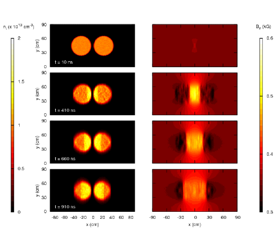
Figure 18: Simulation (2D) of two counter-propagating plasma jets with a 350-G magnetic field in the $+y$ direction. Ion density and $B_{y}$ contours are shown at various times.

As a final simulation, we consider a 2D simulation with more realistic density gradients. The 350-G field is in the $+z$ direction. The initial $n_{i}$ contours can be seen in the top left of Fig. 19. From the $n_{i}$ and $B_{z}$ contours at later times, we note that it is difficult to clearly see the propagation front in the density contours as they are imposed on top of the initial gradient, but the magnetic field front of the shock is clearly seen in the field contours. The simulation results from Figs. 9 and 18 demonstrate that shock structure can be observed in magnetized jets with realistic density gradients.

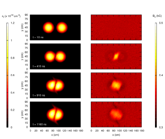
Figure 19: Simulation (2D) of two counter-propagating plasma jets with a 350-G magnetic field in the $+y$ direction. Ion density and $B_{z}$ contours are shown at various times. In contrast to Fig. 17, the jets have finite initial density gradients.

IV Conclusions

We have performed 1D and 2D PIC simulations of hydrogen plasma jet propagation and head-on merging. In the parameter regime of the LANL experiment, unmagnetized collisionless shocks could not be detected in the simulation results. The simulations do demonstrate the formation of magnetized (perpendicular) collisionless shocks when $v_{j}<v_{A}$ ($\beta\ll 1$). This requires that the jets be immersed in a field $\sim 0.1$–1 kG. Simulations predict $M\approx 1$–2 in this parameter range. Non-shock jet interactions (i.e., the Alfvén wave propagation discussed in Sec. III.3.4) are also observed in the simulations as well as ion kinetic effects. These simulation confirm that the application of an appropriate magnetic field to the LANL experiment is required. Some simple calculations as well as preliminary simulations show that an applied field cannot fully diffuse into the oncoming jets on time scales $<1$ $\mu$s. For this reason the jets need to be “born” in the magnetic field or penetrate into the field by some other mechanism than magnetic diffusion Baker and Hammel (1965). Since applied fields were shown to suppress ambipolar diffusion [see Fig. 4(c)], it would be valuable to perform a large-scale 2D jet propagation simulation to see how jets would evolve when born or injected into applied fields. Larger-scale 2D or 3D simulations require better spatial resolution to avoid numerical difficulties for longer simulation times ($t>1$ $\mu$s). Although not considered in this paper, we point out that the LANL experiment should also be able to observe unmagnetized collisional shocks with higher density merging jets and has observed such phenomena Merritt et al. .