Two-year monitoring of intra-day variability of quasar 1156+295 at 4.8 GHz

Abstract

Aims. The quasar 1156+295 (4C +29.45) is one of the targets in the Urumqi monitoring program which aimed to search for evidence of annual modulation in the timescales of intra-day variable (IDV) sources.

Methods. The IDV observations of 1156+295 were carried out nearly monthly from October 2007 to October 2009, with the Urumqi 25m radio telescope at 4.8 GHz.

Results. The source has shown prominent IDV of total flux density in most observing sessions with variability timescales of $\leq$ 1 day at 4.8 GHz. The estimated IDV timescales seem to follow an annual cycle that can be fitted with an anisotropic interstellar scintillation (ISS) model suggesting that a significant part of the flux density variations is due to ISS. The source underwent a dramatic flare in 2008. We studied the possible consequences of the flare on the IDV of 1156+295 by comparing the changes in its IDV characteristics with the evolution of the 43 GHz Very Long Baseline Array (VLBA) core size of the source. The table 3 that contains all flux measurements is only available in electronic form at the CDS via anonymous ftp to cdsarc.u-strasbg.fr (130.79.128.5) or via http://cdsweb.u-strasbg.fr/cgi-bin/qcat?J/A+A/.

Conclusions. The quasar 1156+295 shows evidence for an annual modulation of its IDV timescales at 4.8 GHz, the ISS-induced IDV timescales and variability strength might be affected by the overall activity state of the source core. More frequent IDV and VLBI measurements are required to confirm the relation between the IDV appearance and the core-size evolution of the source.

1 Introduction

Intra-day variability (IDV) has been observed in compact, radio-loud active galactic nuclei (AGNs) over a wide range of the electromagnetic spectrum. At centimeter wavelengths it was first discovered in the mid-1980s (Witzel et al. 1986; Heeschen et al. 1987). Subsequent investigations showed that 25% to 50% of flat-spectrum radio sources (Quirrenbach et al. 1992; Lovell et al. 2008) and $\sim$60% of bright Fermi blazars (Liu et al. 2011, 2012a) are radio intra-day variables. Both source-intrinsic and source-extrinsic mechanisms have been proposed as possible explanations of the variability (see Wagner & Witzel 1995). Source-intrinsic models attribute IDV to flux density variations taking place directly in the AGNs. A simultaneous change in the variability characteristics of radio and optical light curves detected in the blazar S5 0716+714 during a four-week monitoring campaign (see Quirrenbach et al. 1991) is the strongest argument in favor of the possibility of source-intrinsic IDV at radio bands. More recently, in a multifrequency campaign on the same object, Fuhrmann et al. (2008) found stronger IDV at short-centimeter and millimeter bands than at longer wavelengths, confirming that the variability is probably intrinsic to the source. The main issue with source-intrinsic explanations is that, because of causality arguments, flux density variations on timescales of less than one day imply very high brightness temperatures for the emitting components (Qian et al. 1991), violating the inverse-Compton limit $10^{12}$K (Kellermann & Pauliny-Toth 1969). Source-extrinsic models, which attribute IDV to propagation effects, mainly due to interstellar scintillation (ISS) in our Galaxy (e.g., Rickett et al. 1995; Dennett-Thorpe & de Bruyn 2000; Bignall et al. 2003; Rickett 2007), are less affected by the brightness temperature problem.

In both source-intrinsic and -extrinsic models, the essential characteristic of an IDV source is the very small size of the emitting region. Since the light emitted by a very compact source is expected to scintillate after crossing a plasma screen, the idea that the turbulent interstellar medium may be the cause of most of the detected IDV is not only reasonable, but almost inevitable. An interesting implication of the standard ISS models is that the timescale of the variability changes according to the relative velocity between the Earth and the screen. Because of the orbital motion of the Earth around the Sun, this velocity changes across the year. If IDV is caused by ISS, the variability timescales should undergo a one-year periodic cycle, commonly referred to as the annual modulation of the IDV timescales.

The relationship which binds IDV to very small emitting regions also explains how the IDV phenomenon reflects AGNs. All IDV sources are flat-spectrum radio-loud AGNs (the most compact among the AGNs), and almost all are blazars. Blazars are highly variable through the whole electromagnetic spectrum, from the radio to gamma-ray band; in the light of the AGN unified model (Urry & Padovani 1995), this is commonly interpreted in terms of the beaming effect of a relativistic jet oriented very close to our line of sight. The smaller the angle between the jet and the line of sight, the smaller the apparent size of the emitting region. Gamma-ray loud blazars are supposed to be more compact than others, therefore a correlation between $\gamma$-ray emission and IDV characteristics of blazars would naturally be expected. Looking at the sources detected by the Fermi $\gamma$-ray satellite, it appears that the IDV detection rate is higher in Fermi blazars than in non-Fermi blazars (Liu et al. 2012a).

The arguments above suggest how strongly the IDV characteristics of an AGN should relate to the structure of its emitting region. Strong IDV was found in the visibilities of the VLBA data at 15 GHz of the quasar 1156+295 by Savolainen & Kovalev (2008), and it was explained with ISS. Furthermore, it is likely that the emission of a new component in the jet of an IDV source leads to an enlargement of the size of the scintillating region, inducing a prolongation of the IDV timescale or even the quenching of the IDV, as might have occurred in 0917+624 (Krichbaum et al. 2002; Liu et al. 2013). Multiple scintillating regions related to the appearance of new emitting components could be at work in some IDV sources (e.g., in J1819+3845, Macquart & de Bruyn 2007). These variations in the structure of IDV sources may reflect on their average flux density emission, as they are most likely associated with strong outburst phases (Marchili et al. 2012).

Long-term monitoring of IDV sources is crucial for finding both annual cycles in the IDV timescales, which could prove to be a possible ISS origin of the IDV, and possible correlations between the IDV characteristics and the flaring/quiescent state of a source.

We have carried out a monitoring program for a sample of IDV sources with the Urumqi 25m radio telescope at 4.8 GHz, aiming to search for evidence of annual modulation in the timescales of known IDV sources. At least three IDV sources (J1128+592, S4 0954+658, and S5 0716+714) in the monitoring program have shown annual modulation patterns which favor an ISS origin of their variability (Gabányi et al. 2007; Marchili et al. 2012; Liu et al. 2012b). The source 1156+295 (4C +29.45, with redshift of 0.724488, and Galactic coordinates l=199.41°, b=+78.37°) is a flat-spectrum radio quasar, and also a Fermi $\gamma$-ray source. It is one of the targets of our monitoring campaign and was observed nearly on a monthly basis from October 2007 to October 2009. In this paper, we present the results of the IDV observations of 1156+295, analyze the variability timescales and discuss possible effects of the source flare that peaked around March 2009 on the IDV.

2 Observation and data reduction

The Urumqi IDV observation campaign was carried out from August 2005 to January 2010 with the Urumqi 25m radio telescope, at a frequency of 4.8 GHz. Observing sessions of three to five days were typically scheduled once a month. The observing strategy and the detailed calibration method were described in Marchili et al. (2010); the accuracy of the calibrated data is of the order of 0.5% in normal weather conditions. The quasar 1156+295 was included in our monitoring program in late 2007, observed in 18 observing sessions from October 2007 to October 2009. One observing session was too short ($<$ 1 day) to provide a reasonable estimation of the variability characteristics, therefore it was discarded. An example of a light curve for 1156+295 is shown in Fig. 1.

To quantify the variability of the source in each observing session, we calculated the rms flux density, the rms flux density over mean flux density (the so-called modulation index, $m$), and the relative variability amplitude $Y$, defined as $Y=3\sqrt{m^{2}-m_{0}^{2}}$, where $m_{0}$ is the mean modulation index of all calibrators. This last parameter is meant to provide an estimation of the true variability for the given observing session, after removing the residual noise that still affects the data. To evaluate the significance of the variability we used a reduced chi-squared test. The whole procedure follows the strategy proposed by Kraus et al. (2003).

The results of the statistical analysis for each observing session are listed in Table 1, along with basic information about the observing sessions themselves. Table 1 also includes the estimates of the variability timescales which are obtained from the structure function (SF) introduced in the next section. The columns give: (1) the epoch; (2) the day of year (DoY); (3) and (4) the duration of observation and the effective number of data points; (5) and (6) the IDV timescale and relative error from the SF; (7), (8), and (9) the modulation index of calibrators, the modulation index, and the relative variability amplitude $Y$ of 1156+295; (10) the source average flux density and the rms flux density; (11) the reduced $\chi^{2}$ for the variability.

Table 1: The observational information and the results derived from the IDV observations at 4.8 GHz.

1	2	3	4	5	6	7	8	9	10	11
Start Day	DoY	dur	NP	$\tau_{sf}$	error	$m_{0}$	$m$	$Y$	$\overline{S}_{4.8GHz}\pm rms$	$\chi_{r}^{2}$
		(d)		(d)		[%]	[%]	[%]	(Jy)
13 Oct 2007	287	3.0	36	0.8	0.2	0.4	2.4	7.1	1.022$\pm$0.024	17.12
21 Dec 2007	356	3.2	44	0.3	0.1	0.4	6.4	19.2	0.979$\pm$0.063	148.33
25 Feb 2008	57	2.9	28	0.3	0.1	0.6	3.5	10.3	0.963$\pm$0.034	13.06
22 Mar 2008	82	3.0	39	0.4	0.1	0.4	6.5	19.5	1.032$\pm$0.067	134.91
22 Apr 2008	113	3.1	36	0.4	0.1	0.5	5.7	17.0	1.058$\pm$0.060	91.16
21 Jun 2008	173	3.5	63	0.4	0.1	0.5	6.5	19.4	1.246$\pm$0.081	151.98
18 Jul 2008	200	4.8	44	0.3	0.1	0.6	2.9	8.5	1.417$\pm$0.041	16.85
20 Aug 2008	233	5.0	78	0.5	0.1	0.6	3.2	9.6	1.568$\pm$0.050	31.23
13 Sep 2008	257	3.0	45	0.8	0.2	0.4	3.9	11.6	1.685$\pm$0.066	51.91
6 Nov 2008	311	3.6	26	0.3	0.1	0.6	1.7	4.8	2.074$\pm$0.035	5.06
22 Dec 2008	357	2.3	26	0.4	0.1	0.4	1.2	3.4	2.428$\pm$0.028	3.67
11 Jan 2009	12	2.6	38	0.5	0.1	0.4	3.4	10.1	2.628$\pm$0.090	33.67
21 Mar 2009	81	4.9	63	0.4	0.1	0.4	1.9	5.6	2.740$\pm$0.051	10.90
19 Apr 2009	110	5.4	54	0.3	0.1	0.5	1.3	3.6	2.629$\pm$0.033	4.43
25 Jun 2009	177	2.6	26	0.5	0.1	0.6	1.4	3.8	2.382$\pm$0.034	5.93
22 Sep 2009	266	5.5	54	-	-	0.6	0.8	1.6	1.817$\pm$0.014	1.60
9 Oct 2009	283	2.3	30	0.5	0.1	0.4	1.1	3.1	1.745$\pm$0.019	2.85

3 IDV analysis and ISS model-fit

With the chi-squared test of the $\chi_{r}^{2}$ reported in Table 1, the quasar 1156+295 shows IDV in most of the observing sessions at a confidence level of $\geq\,99.9$ %, except for the session of September 2009. The variability amplitude $Y$ varies from about 3% to 20%, while the peak-to-trough variations in the light curves, in some cases, are as high as 25% (see Fig. 1).

3.1 IDV timescale estimate

The characteristic timescale of the IDV in 1156+295 was estimated using the first-order SF analysis (Simonetti et al. 1985). The value returned by the SF for a given time-lag $\tau$ is proportional to the variance of the signal calculated using all the pairs of data-points with time-separation $\sim\tau$. If the variability of a signal has a characteristic timescale $\tau_{sf}$, its variance should fluctuate around a constant value for any $\tau>\tau_{sf}$. Above the noise level, the SF rises monotonically with a power-law shape, reaching a plateau at the characteristic timescale $\tau_{sf}$. Sometimes the structure function may show more than one plateau, indicating the existence of multiple variability timescales. In these cases, we identified the characteristic timescale with the shortest plateau (Marchili et al. 2012). The error of the IDV timescale is estimated by considering the uncertainties in the evaluation of both the SF saturation level and the power-law fit; generally, longer timescales are affected by relatively larger errors.

In Fig. 2, we provide an example of a structure function for the light curve in December 2007 (Fig. 1), with the arrow marking the timescale area. The resulting IDV timescales range from $\sim$ 0.3 to 1.0 day, typically around 0.4$\pm$0.1 day as listed in Table 1.

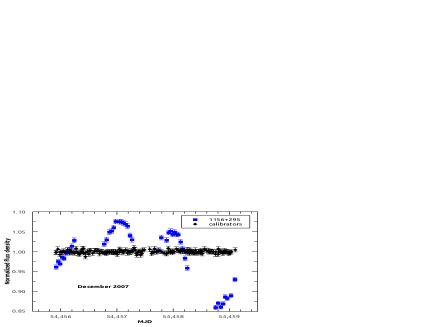
Figure 1: Normalized light curves of quasar 1156+295 (square) and calibrators (diamond) in December 2007 at 4.8 GHz.

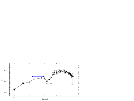
Figure 2: Structure function plot for the 2007 December data of 1156+295 at 4.8 GHz.

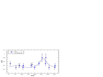
Figure 3: Annual modulation plot of the IDV of 1156+295 at 4.8 GHz, with the best-fit anisotropic ISS model for the IDV timescale.

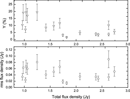
Figure 4: Relative variability amplitude $Y$ (upper panel) and rms flux density (lower panel) versus total flux density at 4.8 GHz.

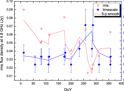
Figure 5: The rms flux density and the IDV timescale at 4.8 GHz versus day of year.

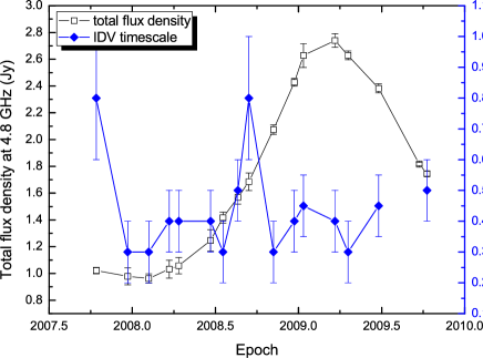
Figure 6: Total flux density and the IDV timescale at 4.8 GHz versus observing epoch.

3.2 Annual modulation model fit

To investigate the possible existence of an annual modulation in the timescales, we fitted a model that relies on the formalism introduced by Coles and Kaufman (1978), developed in Qian & Zhang (2001), and updated to take into account the case of anisotropic scattering (Bignall et al. 2006; Gabányi et al. 2007; see Marchili et al. 2012 for more details). Figure 3 displays the IDV timescales from the SF method versus day of year. According to the anisotropic ISS model, the variation of the IDV as a function of DoY depends on the orientation of the elliptical scintillation pattern (described by the vector ${\bf\hat{s}}=(\mathrm{cos\theta,sin\theta})$), the relative velocity between the scattering screen and the Earth $\bf v\mathrm{(DoY)}=\bf v_{\mathrm{ISS}}-\bf v_{\oplus}\mathrm{(DoY)}$, the distance to the screen D, the source’s angular size $\theta_{s}$, and the anisotropy factor r:

$$\tau(\mathrm{DoY})=\frac{\theta_{s}\mathrm{D}\cdot\sqrt{\mathrm{r}}}{\sqrt{{\mathrm{v}^{2}(\mathrm{DoY})+(\mathrm{r}^{2}-1)\,({\bf v(\mathrm{DoY})\times\hat{s}})^{2}}}}.$$ (1)

The algorithm for the least-squares fitting of the time scales uses five free parameters: the relative velocity between the scattering screen and the Earth ${\bf v}$ projected onto the right ascension and the declination coordinates which allows one to fit the screen velocity ($\bf v_{\mathrm{ISS},\alpha}$ and $\bf v_{\mathrm{ISS},\delta}$) relative to the local standard of rest (LSR), since the Earth’s velocity is known with respect to the LSR; the distance to the screen; the anisotropy degree; and the anisotropy angle $\theta$ (measured from east through north), which is derived from the vectorial product ${\bf v(\mathrm{DoY})\times\hat{s}}$. We note that the distance cannot be unambiguously calculated, unless the source angular size is known. For a rough estimation of D, we assumed as an educated guess $\theta_{s}=70\mu as$.

The parameters that best fit the timescales of 1156+295, along with the respective reduced chi-squared values, are reported in Table 2, and the anisotropic ISS model fitted curve is shown in Fig. 3 for the IDV timescales. The IDV timescales show evidence in favor of a seasonal cycle, with a remarkable slow-down between DoY 250 and 290. The screen has a relatively high velocity (with respect to LSR), at a distance of 0.17$\pm$0.04 kpc. The screen appears strongly anisotropic, with an anisotropy ratio of 10.0$\pm 1.0$ and an anisotropy angle of 170°$\pm$10°(measured from east through north). Such highly anisotropic scattering is not rare; the three known fast (intra-hour) scintillating sources all show evidence of highly anisotropic scintillation patterns (i.e., quasar PKS 0405$-$385, Rickett et al. 2002; quasar J1819+3845, Dennett-Thorpe & de Bruyn 2003; quasar PKS 1257$-$326, Bignall et al. 2006). In our case, quasar 1156+295 has a typical timescale of $\sim$ 0.4 day, placing it between the intra-hour variables and the classical IDV sources. It is claimed that in the one-dimensional scintillation model proposed by Walker et al. (2009) an anisotropy degree can be as high as $10^{5}$. For high Galactic-latitude scintillating sources like 1156+295, the highly anisotropic plasma turbulence may be concentrated in relatively thin layers lying along the boundary of clouds (Linsky et al. 2008), for example.

We also tried to fit the IDV timescales with an isotropic ISS model; it returns a lower velocity of the scattering screen $v_{\alpha}=-$70$\pm 30$ km/s and $v_{\delta}=$25$\pm 15$ km/s, and a larger distance of 0.29$\pm 0.12$ kpc to the screen, as listed in Table 2. Given the lower number of free parameters, the isotropic fit to the timescale provides a larger ${\chi_{r}}^{2}$ than the anisotropic model. In the following, we will focus on the anisotropic ISS model result.

Table 2: Screen parameters estimated from anisotropic and isotropic ISS models for the IDV timescales of 1156+295 at 4.8 GHz.

Method $$v_{\mathrm{ISS},\alpha}$$ Screen Anisotropy Anisotropy

to LSR to LSR distance degree angle

(km/s) (km/s) (kpc) (ratio)

Anisotropic 1.1

Isotropic 2.5

Both the modulation index $m$ and the relative amplitude $Y$ (see Table 1) follow a decreasing trend in the two years of our monitoring campaign; by definition, the two quantities are inversely proportional to total flux density. Their variations may be caused by significant changes either in the rms or in the average flux density which varies considerably because of a strong flare peaking around March 2009 (see, e.g., the relative amplitude $Y$ versus total flux density in Fig. 4, upper panel). Plotting the rms versus average flux density (Fig. 4, lower panel), we do not find any significant correlation between the rms and total flux density. It should be noted that for a given light curve intended as a series of measurements of a given signal, the rms value is influenced both by the characteristics of the signal and by the sampling. The estimated rms of the same signal may vary considerably depending on how densely and uniformly the signal is sampled. We tried to estimate the uncertainty in the reported rms values of the 1156+295 light curves using two independent approaches: 1. In June 2008, the Urumqi observations were performed quasi-simultaneously with the Effelsberg observations. The length and the sampling of the resulting light-curves are significantly different; they can be considered as independent realizations of the same process. Their rms values differ by $\sim$30%. 2. We calculated the running standard deviations over the longest 1156+295 light curves; the time windows were chosen to be comparable to or longer than the variability timescales, to ensure that a significant amount of variability would not be lost. We compared the results obtained for windows with different sizes and samplings, finding a deviation from the average by about 25%. These tests suggest that it is reasonable to consider an uncertainty in the estimated rms values around 30%.

The rms and the IDV timescale are plotted versus DoY in Fig. 5. It appears that the longest timescale lies around the lowest rms flux density, similar to the case of S5 0716+714 (Liu et al. 2012b), implying that the IDV amplitude may be lowest around the timescale that is the slowest in the annual modulation.

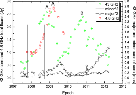
Figure 7: Integrated flux density values (green), the size of the major (times 2 for better display) and minor (times 2) axes of the 43 GHz VLBA core, and the 4.8 GHz total flux density (red) versus observing epoch. The vertical lines indicate the longer IDV timescales and the possible quenching of the variability

(the last vertical line); the letters A and B mark the flares of 1156+295.

4 Discussion of the source flare

As can be seen in Fig. 6, the flux density of 1156+295 underwent a significant flare. The flare appears to start in early 2008 at 4.8 GHz and the flux density monotonically increases to a peak at early 2009. The peak-to-trough variation of flux density is $\sim$ 170%; the long-term variations should be due to a source intrinsic property.

Lovell et al. (2003) first detected the IDV of 1156+295 in three nights with the VLA at 5 GHz, and Lovell et al. (2008) reported the modulation index $m$ of the IDV in this source of 5.8%, 3.4%, 4.6%, and 4.5% (with total flux density of 2.89 Jy, 2.89 Jy, 2.28 Jy, and 1.90 Jy, respectively) for four epochs from 2002 to early 2003 at 5 GHz in the MASIV project. Savolainen & Kovalev (2008) found a significant IDV as high as 40% from peak to trough with a timescale of 2.7 hours in the correlated flux density of 1156+295 in a VLBA observation at 15 GHz on February 5, 2007, and the relative amplitude of the variations is larger than that observed by Lovell et al. (2003) at 5 GHz. Savolainen & Kovalev (2008) argued that this fast IDV at 15 GHz must be due to ISS. In a multi-wavelength campaign, a slower IDV in S5 0716+714 was observed at 10.45 GHz, it has been mainly attributed to a source intrinsic property (Furhmann et al. 2008). At 4.8 GHz in our case, an annual modulation of IDV timescales is obtained for the first time, suggesting that the IDV of 1156+295 at 4.8 GHz is dominated by ISS.

High resolution VLBI images of 1156+295 at 15 GHz have revealed an extremely core dominated jet (with a core fraction of $>$ 90%), with the largest apparent jet speed of 24.74c corresponding to 607$\pm$45 $\mu$as/year (Lister et al. 2009). The inner-jet structures of 1156+295 at 15, 43, and 86 GHz have also been studied with the VLBA observations by Zhao et al. (2011). It is possible that the source structure changes influence the ISS-induced IDV timescale, e.g., the inner-jet position angle changes lead to changes of the projected size of the scintillating component as discussed in Liu et al. (2012b). It is also possible that a new jet leads to a size of the core region (a blend of core and the new jet) close to or larger than the scattering size (i.e., the Fresnel angular scale, see Narayan 1992; Walker 1998), so the IDV timescale could be prolonged, and the scintillation could be quenched, leading to a decrease in the amplitude of the variations, as might have occurred in 0917+624 (Krichbaum et al 2002), for example. After a few months or more, the new jet component moves farther down the jet, expands, and fades, the compact VLBI core becomes dominant again, and the normal scintillation timescale resumes.

We studied the 2008 flare of 1156+295 in some detail, trying to verify its possible effect on the ISS-induced IDV. To investigate the evolution of the source structure, we have tried to model-fit the 43 GHz VLBA core of 1156+295 with two-dimensional elliptical Gaussian model from the Boston University 43 GHz VLBA monitoring data(see Marscher et al. 2012). The result is presented in Fig. 7 (the relative errors of the model-fitted parameters are $\sim$10%), the model fitted core flux density shows that the 2008 flare of 43 GHz core in 1156+295 starts earlier at 43 GHz than the total flux density flare at 4.8 GHz, and a time delay of about five months is evident between the first peak A at 43 GHz and the peak A at 4.8 GHz. The position angle of the model-fitted major axis of the 43 GHz VLBA core ranges from $-10^{\circ}$ to $+20^{\circ}$ with respect to the north; it is not aligned with the anisotropic angle ($\sim$ $-80^{\circ}$ from north) in Table 2. The major and minor axes of the core resulted from the elliptical Gaussian modelfit are in Fig. 7 (multiplied by a factor of 2 for a better display). The major axis is quite stable in the rising phase of the 2008 flare A at 43 GHz, but increases gradually from the down-phase of the flare at 43 GHz. There is an anti-correlation between the major axis and the integrated flux density (coefficient -0.38, with the null hypothesis probability $p$= 0.01) of the core component at 43 GHz. The median value of the major/minor axis ratio is $\sim$2, suggesting the model-fitted inner-jet could not fully account for the high anisotropy degree of the scintillation in Table 2. The minor axis appears to follow a similar trend of the variability of the major axis, with a correlation between the two (coefficient 0.82, with the null hypothesis probability $p$= 8.0E-13). There is no apparent correlation either between the integrated flux density and position angle of the major axis or between the major axis and position angle of the major axis. Statistically, the mean, standard deviation, minimum, median, and maximum value of the minor axes is 68, 33, 13, 65, and 144 in $\mu$as respectively. The mean and median sizes of the minor axes at 43 GHz are comparable to the assumed scintillating component size (70 $\mu$as as mentioned above) in the ISS modelfit at 4.8 GHz. We see that the longer IDV timescales in October 2007 and September 2008 (first two vertical lines in Fig. 7) are in the area of relatively small core size, whereas September 2009 (the last vertical line) is in the area of large core size.

In Fig. 6, no linear correlation (coefficient -0.11, with the null hypothesis, i.e., no correlation probability $p$= 0.68) is found between the IDV timescale and the total flux density, implying that the source flare may have not generally influenced the IDV timescale. The September and October 2009 observations, however, show some characteristics that strongly differentiate them from any previous one. In Sect 3.2, we mentioned that the slowdown phase (between September and October) in the annual modulation of the 1156+295 timescales coincides with a decrease of the rms of the measured flux density. As shown in Fig. 8, the amplitude of the variations observed in September and October 2009 (lower panels) is remarkably lower than in October 2007 and September 2008 (upper panels). In September 2009 the measured variability is comparable with the residual noise in the calibrators, so that it is impossible to estimate a variability timescale. This could be the consequence of a characteristic timescale that is considerably longer than the ones estimated in the same period of previous years, and/or the effect of a quenching of the scattering. In October 2009 the variations in the flux density are visible again, indicating that the variability timescale is comparable to the observation duration, but the amplitude of the variations is still lower than in previous years.

Considering the time delay between the peaks of the flare at 43 and 4.8 GHz, we may hypothesize that the source’s angular size at 4.8 GHz could reach its peak a few months later than at 43 GHz, probably around the end of 2009. It is therefore possible that the peculiarities of the variability characteristics of 1156+295 in September and October 2009 have to do with structural changes in the source’s emitting region.

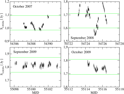
Figure 8: The light curves of 1156+295 during the slowdown phase of the annual modulation cycle. The green lines show the amplitude of the peak-to-peak variation in October 2007.

5 Summary

We have carried out nearly monthly IDV observations of quasar 1156+295 in two years, with the Urumqi 25m radio telescope at 4.8 GHz, and the source has shown prominent IDV in most observing sessions. We estimate the IDV timescale with the method of structure function analysis. The IDV timescales stacking through the day of year can be best-fitted with an anisotropic ISS model, and although the data are relatively sparse, the result is positive in favor of an annual modulation of the IDV timescales, suggesting at least a significant part of the flux density variations are due to ISS. The source underwent a dramatic flare peaking around March 2009 at 4.8 GHz. We analyzed the flux density and size evolution of the model-fitted VLBA core component at 43 GHz to find possible influences on the IDV of the source. We hypothesize that the very low variability amplitudes measured in September and October 2009 may be the consequence of the increased source size related to the flare.

- (1) Bignall, H. E., Jauncey, D. L., Lovell, J. E. J., et al. 2003, ApJ, 585, 653
- (2) Bignall, H. E., Macquart, J.-P., Jauncey, D. L., et al. 2006, ApJ, 652, 1050
- (3) Coles, W. A. & Kaufman, J. J. 1978, Radio Science, 13, 591
- (4) Dennett-Thorpe, J. & de Bruyn, A. G. 2003, A&A, 404, 113
- (5) Dennett-Thorpe, J. & de Bruyn, A. G. 2000, ApJ, 529, L65
- (6) Fuhrmann, L., Krichbaum, T. P., Witzel, A., et al. 2008, A&A, 490, 1019
- (7) Gabányi, K. É., Marchili, N., Krichbaum, T. P., et al. 2007, A&A, 470, 83
- (8) Heeschen, D. S., Krichbaum, T., Schalinski, C. J., et al. 1987, AJ, 94, 1493
- (9) Kellermann, K. I. & Pauliny-Toth, I. I. K. 1969, ApJ, 155, L71
- (10) Krichbaum, T. P., Kraus, A., Fuhrmann, L., Cimò, G., Witzel, A. 2002, PASA, 19, 14
- (11) Kraus, A., Krichbaum, T. P., Wegner, R., et al. 2003, A&A, 401, 161
- (12) Linsky, J. L., Rickett, B. J., Redfield, S. 2008, ApJ, 675, 413
- (13) Lister, M. L., Cohen, M. H., Homan, D. C., et al. 2009, AJ, 138, 1874
- (14) Liu, X., Ding, Z., Liu, J., Marchili, N., Krichbaum, T. P. 2011, J.Astrophys.Astr., 32, 29
- (15) Liu, X., Song, H.-G., Liu, J., et al. 2012a, RAA, 12, 147
- (16) Liu, X., Song, H.-G., Marchili, N., et al. 2012b, A&A, 543, A78
- (17) Liu, X., Li, Q.-W., Krichbaum, T. P., Aller, M. F., Aller, H. D. 2013, Ap&SS, 346, 15
- (18) Lovell, J. E. J., Jauncey, D. L., Bignall, H. E., et al. 2003, AJ, 126, 1699
- (19) Lovell, J. E. J., Rickett, B. J., Macquart, J.-P., et al. 2008, ApJ, 689, 108
- (20) Macquart, J.-P. & de Bruyn, A. G. 2007, MNRAS, 380, L20
- (21) Marchili, N., Martí-Vidal, I., Brunthaler, A., et al. 2010, A&A, 509, A47
- (22) Marchili, N., Krichbaum, T. P., Liu, X., et al. 2012, A&A, 542, A121
- (23) Marscher, A. P., Jorstad, S. G., Agudo, I., MacDonald, N. R., Scott, T. L. 2012, Fermi & Jansky Proceedings - eConf C1111101
- (24) Narayan, R. 1992, Royal Society of London Philosophical Transactions Series A, 341, 151
- (25) Qian, S. J., Quirrenbach, A., Witzel, A., et al. 1991, ApJ, 241, 15
- (26) Qian, S.-J. & Zhang, X.-Z. 2001, Chinese J. Astron. Astrophys., 1, 133
- (27) Quirrenbach, A., Witzel, A., Krichbaum, T. P., et al. 1992, A&A, 258, 279
- (28) Quirrenbach, A., Witzel, A., Wagner, S., et al. 1991, ApJ, 372, L71
- (29) Rickett, B. J., Quirrenbach, A., Wegner, R., Krichbaum, T. P., Witzel, A. 1995, A&A, 293, 479
- (30) Rickett, B. J. (2007) ‘Interstellar scintillation: observational highlights’, Astronomical & Astrophysical Transactions, 26:6, 429
- (31) Rickett, B. J., Kedziora-Chudczer, L., Jauncey, D. L. 2002, ApJ, 581, 103
- (32) Savolainen, T. & Kovalev, Y. Y. 2008, A&A, 489, 33
- (33) Simonetti, J. H., Cordes, J. M., Heeschen, D. S. 1985, ApJ, 296, 46
- (34) Urry, C. M. & Padovani, P. 1995, PASP, 107, 803
- (35) Wagner, S. J. & Witzel, A. 1995, ARA&A, 33, 163
- (36) Walker, M. A. 1998, MNRAS, 294, 307
- (37) Walker, M. A., de Bruyn, A. G., Bignall, H. E. 2009, MNRAS, 397, 447
- (38) Witzel, A., Heeschen, D. S., Schalinski, C., Krichbaum, T. 1986, Mitteilungender Astronomischen Gesellschaft Hamburg, 65, 239
- (39) Zhao, W., Hong, X.-Y., An, T., et al. 2011, A&A, 529, A113