To Reserve or Not to Reserve: Optimal Online Multi-Instance Acquisition in IaaS Clouds

Abstract

Infrastructure-as-a-Service (IaaS) clouds offer diverse instance purchasing options. A user can either run instances on demand and pay only for what it uses, or it can prepay to reserve instances for a long period, during which a usage discount is entitled. An important problem facing a user is how these two instance options can be dynamically combined to serve time-varying demands at minimum cost. Existing strategies in the literature, however, require either exact knowledge or the distribution of demands in the long-term future, which significantly limits their use in practice. Unlike existing works, we propose two practical online algorithms, one deterministic and another randomized, that dynamically combine the two instance options online without any knowledge of the future. We show that the proposed deterministic (resp., randomized) algorithm incurs no more than $2-\alpha$ (resp., $e/(e-1+\alpha)$) times the minimum cost obtained by an optimal offline algorithm that knows the exact future a priori, where $\alpha$ is the entitled discount after reservation. Our online algorithms achieve the best possible competitive ratios in both the deterministic and randomized cases, and can be easily extended to cases when short-term predictions are reliable. Simulations driven by a large volume of real-world traces show that significant cost savings can be achieved with prevalent IaaS prices.

I Introduction

Enterprise spending on Infrastructure-as-a-Service (IaaS) cloud is on a rapid growth path. According to [1], the public cloud services market is expected to expand from $109 billion in 2012 to $207 billion by 2016, during which IaaS is the fastest-growing segment with a 41.7% annual growing rate [2]. IaaS cost management therefore receives significant attention and has become a primary concern for IT enterprises.

Maintaining optimal cost management is especially challenging, given the complex pricing options offered in today’s IaaS services market. IaaS cloud vendors, such as Amazon EC2, ElasticHosts, GoGrid, etc., apply diverse instance (i.e., virtual machine) pricing models at different commitment levels. At the lowest level, cloud users launch on-demand instances and pay only for the incurred instance-hours, without making any long-term usage commitments, e.g., [3, 4, 5]. At a higher level, there are reserved instances wherein users prepay a one-time upfront fee and then reserve an instance for months or years, during which the usage is either free, e.g., [4, 5], or is priced under a significant discount, e.g., [3]. Table I gives a pricing example of on-demand and reserved instances in Amazon EC2.

Acquiring instances at the cost-optimal commitment level plays a central role for cost management. Simply operating the entire load with on-demand instances can be highly inefficient. For example, in Amazon EC2, three years of continuous on-demand service cost 3 times more than reserving instances for the same period [3]. On the other hand, naively switching to a long-term commitment incurs a huge amount of upfront payment (more than 1,000 times the on-demand rate in EC2 [3]), making reserved instances extremely expensive for sporadic workload. In particular, with time-varying loads, a user needs to answer two important questions: (1) when should I reserve instances (timing), and (2) how many instances should I reserve (quantity)?

TABLE I: Pricing of on-demand and reserved instances (Light Utilization, Linux, US East) in Amazon EC2, as of Feb. 10, 2013.

Instance Type	Pricing Option	Upfront	Hourly
Standard Small	On-Demand	$0	$0.08
	1-Year Reserved	$69	$0.039
Standard Medium	On-Demand	$0	$0.16
	1-Year Reserved	$138	$0.078

Recently proposed instance reservation strategies, e.g., [6, 7, 8], heavily rely on long-term predictions of future demands, with historic workloads as references. These approaches, however, suffer from several significant limitations in practice. First, historic workloads might not be available, especially for startup companies who have just switched to IaaS services. In addition, not all workloads are amenable to prediction. In fact, it is observed in real production applications that workload is highly variable and statistically nonstationary [9, 10], and as a result, history may reveal very little information about the future. Moreover, due to the long span of a reservation period (e.g., 1 to 3 years in Amazon EC2), workload predictions are usually required over a very long period of time, say, years. It would be very challenging, if not impossible, to make sufficiently accurate predictions over such a long term. For all these reasons, instance reservations are usually made conservatively in practice, based on empirical experiences [11] or professional recommendations, e.g., [12, 13, 14].

In this paper, we are motivated by a practical yet fundamental question: Is it possible to reserve instances in an online manner, with limited or even no a priori knowledge of the future workload, while still incurring near-optimal instance acquisition costs? To our knowledge, this paper represents the first attempt to answer this question, as we make the following contributions.

With dynamic programming, we first characterize the optimal offline reservation strategy as a benchmark algorithm (Sec. III), in which the exact future demand is assumed to be known a priori. We show that the optimal strategy suffers “the curse of dimensionality” [15] and is hence computationally intractable. This indicates that optimal instance reservation is in fact very difficult to obtain, even given the entire future demands.

Despite the complexity of the reservation problem in the offline setting, we present two online reservation algorithms, one deterministic and another randomized, that offer the best provable cost guarantees without any knowledge of future demands beforehand. We first show that our deterministic algorithm incurs no more than $2-\alpha$ times the minimum cost obtained by the benchmark optimal offline algorithm (Sec. IV), and is therefore $(2-\alpha)$-competitive, where $\alpha\in[0,1]$ is the entitled usage discount offered by reserved instances. This translates to a worst-case cost that is 1.51 times the optimal one under the prevalent pricing of Amazon EC2. We then establish the more encouraging result that, our randomized algorithm improves the competitive ratio to $e/(e-1+\alpha)$ in expectation, and is 1.23-competitive under Amazon EC2 pricing (Sec. V). Both algorithms achieve the best possible competitive ratios in the deterministic and randomized cases, respectively, and are simple enough for practical implementations. Our online algorithms can also be extended to cases when short-term predictions into the near future are reliable (Sec. VI).

In addition to our theoretical analysis, we have also evaluated both proposed online algorithms via large-scale simulations (Sec. VII), driven by Google cluster-usage traces [16] with 40 GB workload demand information of 933 users in one month. Our simulation results show that, under the pricing of Amazon EC2 [3], our algorithms closely track the demand dynamics, realizing substantial cost savings compared with several alternatives.

Though we focus on cost management of acquiring compute instances, our algorithms may find wide applications in the prevalent IaaS services market. For example, Amazon ElastiCache [17] also offers two pricing options for its web caching services, i.e., the On-Demand Cache Nodes and Reserved Cache Nodes, in which our proposed algorithms can be directly applied to lower the service costs.

II Optimal Cost Management

We start off by briefly reviewing the pricing details of the on-demand and reservation options in IaaS clouds, based on which we formulate the online instance reservation problem for optimal cost management.

II-A On-demand and Reservation Pricing

On-Demand Instances: On-demand instances let users pay for compute capacity based on usage time without long-term commitments, and are uniformly supported in leading IaaS clouds. For example, in Amazon EC2, the hourly rate of a Standard Small Instance (Linux, US East) is $0.08 (see Table I). In this case, running it on demand for 100 hours costs a user $8.

On-demand instances resemble the conventional pay-as-you-go model. Formally, for a certain type of instance, let the hourly rate be $p$. Then running it on demand for $h$ hours incurs a cost of $ph$. Note that in most IaaS clouds, the hourly rate $p$ is set as fixed in a very long time period (e.g., years), and can therefore be viewed as a constant.

Reserved Instances: Another type of pricing option that is widely supported in IaaS clouds is the reserved instance. It allows a user to reserve an instance for a long period (months or years) by prepaying an upfront reservation fee, after which, the usage is either free, e.g., ElasticHosts [4], GoGrid [5], or is priced with a heavy discount, e.g., Amazon EC2 [3]. For example, in Amazon EC2, to reserve a Standard Small Instance (Linux, US East, Light Utilization) for 1 year, a user pays an upfront $69 and receives a discount rate of $0.039 per hour within 1 year of the reservation time, as oppose to the regular rate of $0.08 (see Table I). Suppose this instance has run 100 hours before the reservation expires. Then the total cost incurred is $69 + 0.039$\times$100 = $72.9.

Reserved instances resemble the wholesale market. Formally, for a certain type of reserved instance, let the reservation period be $\tau$ (counted by the number of hours). An instance that is reserved at hour $i$ would expire before hour $i+\tau$. Without loss of generality, we assume the reservation fee to be $1$ and normalize the on-demand rate $p$ to the reservation fee. Let $\alpha\in[0,1]$ be the received discount due to reservation. A reserved instance running for $h$ hours during the reservation period incurs a discounted running cost $\alpha ph$ plus a reservation fee, leading to a total cost of $1+\alpha ph$. In the previous example, the normalized on-demand rate $p=0.08/69$; the received discount due to reservation is $\alpha=0.039/0.08=0.49$; the running hour $h=100$; and the normalized overall cost is

$$1+\alpha ph=72.9/69~{}.$$

In practice, cloud providers may offer multiple types of reserved instances with different reservation periods and utilization levels. For example, Amazon EC2 offers 1-year and 3-year reservations with light, medium, and high utilizations [3]. For simplicity, we limit the discussion to one type of such reserved instances chosen by a user based on its rough estimations. We also assume that the on-demand rate is far smaller than the reservation fee, i.e., $p\ll 1$, which is always the case in IaaS clouds, e.g., [3, 4, 5].

II-B The Online Instance Reservation Problem

In general, launching instances on demand is more cost efficient for sporadic workload, while reserved instances are more suitable to serve stable demand lasting for a long period of time, for which the low hourly rate would compensate for the high upfront fee. The cost management problem is to optimally combine the two instance options to serve the time-varying demand, such that the incurred cost is minimized. In this section, we consider making instance purchase decisions online, without any a priori knowledge about the future demands. Such an online model is especially important for startup companies who have limited or no history demand data and those cloud users whose workloads are highly variable and non-stationary — in both cases reliable predictions are unavailable. We postpone the discussions for cases when short-term demand predictions are reliable in Sec. VI.

Since IaaS instances are billed in an hourly manner, we slot the time to a sequence of hours indexed by $t=0,1,2,\dots$ At each time $t$, demand $d_{t}$ arrives, meaning that a user requests $d_{t}$ instances, $d_{t}=0,1,2,\dots$ To accommodate this demand, the user decides to use $o_{t}$ on-demand instances and $d_{t}-o_{t}$ reserved instances. If the previously reserved instances that remain available at time $t$ are fewer than $d_{t}-o_{t}$, then new instances need to be reserved. Let $r_{t}$ be the number of instances that are newly reserved at time $t$, $r_{t}=0,1,2,\dots$ The overall cost incurred at time $t$ is the on-demand cost $o_{t}p$ plus the reservation cost $r_{t}+\alpha p(d_{t}-o_{t})$, where $r_{t}$ is the upfront payments due to new reservations, and $\alpha p(d_{t}-o_{t})$ is the cost of running $d_{t}-o_{t}$ reserved instances.

The cost management problem is to make instance purchase decisions online, i.e., $r_{t}$ and $o_{t}$ at each time $t$, before seeing future demands $d_{t+1},d_{t+2},\dots$ The objective is to minimize the overall instance acquiring costs. Suppose demands last for an arbitrary time $T$ (counted by the number of hours). We have the following online instance reservation problem:

$$\begin{split}\min_{\{r_{t},o_{t}\}}&\quad C=\sum_{t=1}^{T}(o_{t}p+r_{t}+\alpha p(d_{t}-o_{t}))~{},\\ \mbox{s.t.}&\quad o_{t}+\sum_{i=t-\tau+1}^{t}r_{i}\geq d_{t}~{},\\ &\quad o_{t},r_{t}\in\{0,1,2,\dots\},t=1,\dots,T~{}.\end{split}$$ (1)

Here, the first constraint ensures that all $d_{t}$ instances demanded at time $t$ are accommodated, with $o_{t}$ on-demand instances and $\sum_{i=t-\tau+1}^{t}r_{i}$ reserved instances that remain active at time $t$. Note that instances that are reserved before time $t-\tau+1$ have all expired at time $t$, where $\tau$ is the reservation period. For convenience, we set $r_{t}=0$ for all $t\leq 0$.

The main challenge of problem (1) lies in its online setting. Without knowledge of future demands, the online strategy may make purchase decisions that turn out later not to be optimal. Below we clarify the performance metrics to measure how far away an online strategy may deviate from the optimal solution.

II-C Measure of Competitiveness

To measure the cost performance of an online strategy, we adopt the standard competitive analysis [18]. The idea is to bound the gap between the cost of an interested online algorithm and that of the optimal offline strategy. The latter is obtained by solving problem (1) with the exact future demands $d_{1},\dots,d_{T}$ given a priori. Formally, we have

Definition 1 (Competitive analysis)

A deterministic online reservation algorithm $A$ is $c$-competitive ($c$ is a constant) if for all possible demand sequences $\mathbf{d}=\{d_{1},\dots,d_{T}\}$, we have

$$C_{A}(\mathbf{d})\leq c\cdot C_{\mathrm{OPT}}(\mathbf{d})~{},$$ (2)

where $C_{A}(\mathbf{d})$ is the instance acquiring cost incurred by algorithm $A$ given input $\mathbf{d}$, and $C_{\mathrm{OPT}}(\mathbf{d})$ is the optimal instance acquiring cost given input $\mathbf{d}$. Here, $C_{\mathrm{OPT}}(\mathbf{d})$ is obtained by solving the instance reservation problem (1) offline, where the exact demand sequence $\mathbf{d}$ is assumed to know a priori.

A similar definition of the competitive analysis also extends to the randomized online algorithm $A$, where the decision making is drawn from a random distribution. In this case, the LHS of (2) is simply replaced by $\mathbf{E}[C_{A}(\mathbf{d})]$, the expected cost of randomized algorithm $A$ given input $\mathbf{d}$. (See [18] for a detailed discussion.)

Competitive analysis takes an optimal offline algorithm as a benchmark to measure the cost performance of an online strategy. Intuitively, the smaller the competitive ratio $c$ is, the more closely the online algorithm $A$ approaches the optimal solution. Our objective is to design optimal online algorithms with the smallest competitive ratio.

We note that the instance reservation problem (1) captures the Bahncard problem [19] as a special case when a user demands no more than one instance at a time, i.e., $d_{t}\leq 1$ for all $t$. The Bahncard problem models online ticket purchasing on the German Federal Railway, where one can opt to buy a Bahncard (reserve an instance) and to receive a discount on all trips within one year of the purchase date. It has been shown in [19, 20] that the lower bound of the competitive ratio is $2-\alpha$ and $e/(e-1+\alpha)$ for the deterministic and randomized Bahncard algorithms, respectively. Because the Bahncard problem is a special case of our problem (1), we have

Lemma 1

The competitive ratio of problem (1) is at least $2-\alpha$ for deterministic online algorithms, and is at least $e/(e-1+\alpha)$ for randomized online algorithms.

However, we show in the following that the instance reserving problem (1) is by no means a trivial extension to the Bahncard problem, mainly due to the time-multiplexing nature of reserved instances.

II-D Bahncard Extension and Its Inefficiency

A natural way to extend the Bahncard solutions in [19] is to decompose problem (1) into separate Bahncard problems. To do this, we introduce a set of virtual users indexed by 1, 2, …Whenever demand $d_{t}$ arises at time $t$, we view the original user as $d_{t}$ virtual users 1, 2, …, $d_{t}$, each requiring one instance at that time. Each virtual user then reserves instances (i.e., buy a Bahncard) separately to minimize its cost, which is exactly a Bahncard problem.

However, such an extension is highly inefficient. An instance reserved by one virtual user, even idle, can never be multiplexed with another, who still needs to pay for its own demand. For a real user, this implies that it has to acquire additional instances, either on-demand or reserved, even if the user has already reserved sufficient amount of instances to serve its demand, which inevitably incurs a large amount of unnecessary cost.

We learn from the above failure that instances must be reserved jointly and time multiplexed appropriately. These factors significantly complicate our problem (1). Indeed, as we see in the next section, even with full knowledge of the future demand, obtaining an optimal offline solution to (1) is computationally prohibitive.

III The Offline Strategy and Its Intractability

In this section we consider the benchmark offline cost management strategy for problem (1), in which the exact future demands are given a priori. The offline setting is an integer programming problem and is generally difficult to solve. We derive the optimal solution via dynamic programming. However, such an optimal offline strategy suffers from “the curse of dimensionality” [15] and is computationally intractable.

We start by defining states. A state at time $t$ is defined as a $(\tau-1)$-tuple $\mathbf{s}_{t}=(s_{t,1},\dots,s_{t,\tau-1})$, where $s_{t,i}$ denotes the number of instances that are reserved no later than $t$ and remain active at time $t+i$, $i=1,\dots,\tau-1$. We use a $(\tau-1)$-tuple to define a state because an instance that is reserved no later than $t$ will no longer be active at time $t+\tau$ and thereafter. Clearly, $s_{t,1}\geq\dots\geq s_{t,\tau-1}$ as reservations gradually expire.

We make an important observation, that state $\mathbf{s}_{t}$ only depends on states $\mathbf{s}_{t-1}$ at the previous time, and is independent of earlier states $\mathbf{s}_{t-2},\dots,\mathbf{s}_{1}$. Specifically, suppose state $\mathbf{s}_{t-1}$ is reached at time $t-1$. At the beginning of the next time $t$, $r_{t}$ new instances are reserved. These newly reserved $r_{t}$ instances will add to the active reservations starting from time $t$, leading state $\mathbf{s}_{t-1}$ to transit to $\mathbf{s}_{t}$ following the transition equations below:

$$\left\{\begin{array}[]{ll}s_{t,i}=s_{t-1,i+1}+r_{t},&i=1,\dots,\tau-2~{};\\ s_{t,\tau-1}=r_{t}.&\end{array}\right.$$ (3)

Let $V(\mathbf{s}_{t})$ be the minimum cost of serving demands $d_{1},\dots,d_{t}$ up to time $t$, conditioned upon the fact that state $\mathbf{s}_{t}$ is reached at time $t$. We have the following recursive Bellman equations:

$$V(\mathbf{s}_{t})=\min_{s_{t-1}}\big{\{}V(\mathbf{s}_{t-1})+c(\mathbf{s}_{t-1},\mathbf{s}_{t})\big{\}},\quad t>0,$$ (4)

where $c(\mathbf{s}_{t-1},\mathbf{s}_{t})$ is the transition cost, and the minimization is over all states $\mathbf{s}_{t-1}$ that can transit to $\mathbf{s}_{t}$ following the transition equations (3). The Bellman equations (4) indicate that the minimum cost of reaching $\mathbf{s}_{t}$ is given by the minimum cost of reaching a previous state $\mathbf{s}_{t-1}$ plus the transition cost $c(\mathbf{s}_{t-1},\mathbf{s}_{t})$, minimized over all possible previous states $\mathbf{s}_{t-1}$. Let

$$X^{+}=\max\{0,X\}~{}.$$ (5)

The transition cost is defined as

$$c(\mathbf{s}_{t-1},\mathbf{s}_{t})=o_{t}p+r_{t}+\alpha p(d_{t}-o_{t})~{},$$ (6)

where

$$r_{t}=s_{t,\tau-1},$$ (7)

$$o_{t}=(d_{t}-r_{t}-s_{t-1,1})^{+},$$ (8)

and the transition from $\mathbf{s}_{t-1}$ to $\mathbf{s}_{t}$ follows (3). The rationale of (6) is straightforward. By the transition equations (3), state $\mathbf{s}_{t-1}$ transits to $\mathbf{s}_{t}$ by reserving $r_{t}=s_{t,\tau-1}$ instances at time $t$. Adding the $s_{t-1,1}$ instances that have been reserved before $t$, we have $r_{t}+s_{t-1,1}$ reserved instances to use at time $t$. We therefore need $o_{t}=(d_{t}-r_{t}-s_{t-1,1})^{+}$ on-demand instances at that time.

The boundary conditions of Bellman equations (4) are

$$V(\mathbf{s}_{0})=s_{0,1},\quad\mbox{for all $\mathbf{s}_{0}=(s_{0,1},\dots,s_{0,\tau-1})$},$$ (9)

because an initial state $\mathbf{s}_{0}$ indicates that a user has already reserved $s_{0,1}$ instances at the beginning and paid $s_{0,1}$.

With the analyses above, we see that the dynamic programming defined by (3), (4), (6), and (9) optimally solves the offline instance reserving problem (1). Therefore, it gives $C_{\mathrm{OPT}}(\mathbf{d})$ in theory.

Unfortunately, the dynamic programming presented above is computationally intractable. This is because to solve the Bellman equations (4), one has to compute $V(\mathbf{s}_{t})$ for all states $\mathbf{s}_{t}$. However, since a state $\mathbf{s}_{t}$ is defined in a high-dimensional space — recall that $\mathbf{s}_{t}$ is defined as a $(\tau-1)$-tuple — there exist exponentially many such states. Therefore, looping over all of them results in exponential time complexity. This is known as the curse of dimensionality suffered by high-dimensional dynamic programming [15].

The intractability of the offline instance reservation problem (1) suggests that optimal cost management in IaaS clouds is in fact a very complicate problem, even if future demands can be accurately predicted. However, we show in the following sections that it is possible to have online strategies that are highly efficient with near-optimal cost performance, even without any knowledge of the future demands.

IV Optimal Deterministic Online Strategy

In this section, we present a deterministic online reservation strategy that incurs no more than $2-\alpha$ times the minimum cost. As indicated by Lemma 1, this is also the best that one can expect from a deterministic algorithm.

IV-A The Deterministic Online Algorithm

We start off by defining a break-even point at which a user is indifferent between using a reserved instance and an on-demand instance. Suppose an on-demand instance is used to accommodate workload in a time interval that spans a reservation period, incurring a cost $c$. If we use a reserved instance instead to serve the same demand, the cost will be $1+\alpha c$. When $c=1/(1-\alpha)$, both instances cost the same, and are therefore indifferent to the user. We hence define the break-even point as

$$\beta=1/(1-\alpha)~{}.$$ (10)

Clearly, the use of an on-demand instance is well justified if and only if the incurred cost does not exceed the break-even point, i.e., $c\leq\beta$.

Our deterministic online algorithm is summarized as follows. By default, all workloads are assumed to be operated with on-demand instances. At time $t$, upon the arrival of demand $d_{t}$, we check the use of on-demand instances in a recent reservation period, starting from time $t-\tau+1$ to $t$, and reserve a new instance whenever we see an on-demand instance incurring more costs than the break-even point. Algorithm 1 presents the detail.

Algorithm 1 Deterministic Online Algorithm $A_{\beta}$

1.  Let $x_{i}$ be the number of reserved instances at time $i$, Initially, $x_{i}\leftarrow 0$ for all $i=0,1,\dots$

2.  Let $I(X)$ be an indicator function where $I(X)=1$ if $X$ is true and $I(X)=0$ otherwise. Also let $X^{+}=\max\{X,0\}$.

3.  Upon the arrival of demand $d_{t}$, loop as follows:

4.  while $p\sum_{i=t-\tau+1}^{t}I(d_{i}>x_{i})>\beta$ do

5.     Reserve a new instance: $r_{t}\leftarrow r_{t}+1$.

6.     Update the number of reservations that can be used in the future: $x_{i}\leftarrow x_{i}+1$ for $i=t,\dots,t+\tau-1$.

7.     Add a “phantom” reservation to the recent period, indicating that the history has already been “processed”: $x_{i}\leftarrow x_{i}+1$ for $i=t-\tau+1,\dots,t-1$.

8.  end while

9.  Launch on-demand instances: $o_{t}\leftarrow(d_{t}-x_{t})^{+}$.

10.  $t\leftarrow t+1$, repeat from 3.

Fig. 1 helps to illustrate Algorithm 1. Whenever demand $d_{t}$ arises, we check the recent reservation period from time $t-\tau+1$ to $t$. We see that an on-demand instance has been used at time $i$ if demand $d_{i}$ exceeds the number of reservations $x_{i}$ (both actual and phantom), $i=t-\tau+1,\dots,t$. The shaded area in Fig. 1 represents the use of an on-demand instance in the recent period, which incurs a cost of $p\sum_{i=t-\tau+1}^{t}I(d_{i}>x_{i})$. If this cost exceeds the break-even point $\beta$ (line 4 of Algorithm 1), then such use of an on-demand instance is not well justified: We should have reserved an instance before at time $t-\tau+1$ and used it to serve the demand (shaded area) instead, which would have lowered the cost. As a compensation for this “mistake,” we reserve an instance at the current time $t$ (line 5), and will have one more reservation to use in the future (line 6). Since we have already compensated for a misuse of an on-demand instance (the shaded area), we add a “phantom” reservation to the history so that such a mistake will not be counted multiple times in the following rounds (line 7). This leads to an update of the reservation number $\{x_{i}\}$ (see the bottom figure in Fig. 1).

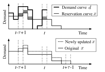
Figure 1: Illustration of Algorithm 1. The shaded area in the top figure shows the use of an on-demand instance in the recent period. An instance is reserved at time $t$ if the use of this on-demand instance is not well justified. The bottom figure shows the corresponding updates of the reservation curve $x$.

Unlike the simple extension of the Bahncard algorithm described in Sec. II-D, Algorithm 1 jointly reserves instances by taking both the currently active reservations (i.e., $x_{t}$) and the historic records (i.e., $x_{i}$, $i<t$) into consideration (line 4), without any knowledge of the future. We will see later in Sec. VII that such a joint reservation significantly outperforms the Bahncard extension where instances are reserved separately.

IV-B Performance Analysis: $(2-\alpha)$-Competitiveness

The “trick” of Algorithm 1 is to make reservations “lazily”: no instance is reserved unless the misuse of an on-demand instance is seen. Such a “lazy behaviour” turns out to guarantee that the algorithm incurs no more than $2-\alpha$ times the minimum cost.

Let $A_{\beta}$ denote Algorithm 1 and let OPT denote the optimal offline algorithm. We now make an important observation, that OPT reserves at least the same amount of instances as $A_{\beta}$ does, for any demand sequence.

Lemma 2

Given an arbitrary demand sequence, let $n_{\beta}$ be the number of instances reserved by $A_{\beta}$, and let $n_{\mathrm{OPT}}$ be the number of instances reserved by OPT. Then $n_{\beta}\leq n_{\mathrm{OPT}}$.

Lemma 2 can be viewed as a result of the “lazy behaviour” of $A_{\beta}$, in which instances are reserved just to compensate for the previous “purchase mistakes.” Intuitively, such a conservative reservation strategy leads to fewer reserved instances. The proof of Lemma 2 is is given in Appendix A.

We are now ready to analyze the cost performance of $A_{\beta}$, using the optimal offline algorithm OPT as a benchmark.

Proposition 1

Algorithm 1 is $(2-\alpha)$-competitive. Formally, for any demand sequence,

$$C_{A_{\beta}}\leq(2-\alpha)C_{\mathrm{OPT}}~{},$$ (11)

where $C_{A_{\beta}}$ is the cost of Algorithm 1 ($A_{\beta}$), and $C_{\mathrm{OPT}}$ is the cost of the optimal offline algorithm OPT.

Proof: Suppose $A_{\beta}$ (resp., OPT) launches $o_{t}$ (resp., $o_{t}^{*}$) on-demand instances at time $t$. Let $\mathrm{Od}(A_{\beta})$ be the costs incurred by these on-demand instances under $A_{\beta}$, i.e.,

$$\mathrm{Od}(A_{\beta})=\sum_{t=1}^{T}o_{t}p~{}.$$ (12)

We refer to $\mathrm{Od}(A_{\beta})$ as the on-demand costs of $A_{\beta}$. Similarly, we define the on-demand costs incurred by OPT as

$$\mathrm{Od}(\mathrm{OPT})=\sum_{t=1}^{T}o_{t}^{*}p~{}.$$ (13)

Also, let

$$\mathrm{Od}(A_{\beta}\backslash\mathrm{OPT})=\sum_{t=1}^{T}(o_{t}-o_{t}^{*})^{+}p$$ (14)

be the on-demand costs incurred in $A_{\beta}$ that are not incurred in OPT. We see

$$\mathrm{Od}(A_{\beta}\backslash\mathrm{OPT})\leq\beta n_{\mathrm{OPT}}$$ (15)

by noting the following two facts: First, demands $\sum_{t=1}^{T}(o_{t}-o_{t}^{*})^{+}$ are served by at most $n_{\mathrm{OPT}}$ reserved instances in OPT. Second, demands that are served by the same reserved instance in OPT incur on-demand costs of at most $\beta$ in $A_{\beta}$ (by the definition of $A_{\beta}$). We therefore bound $\mathrm{Od}(A_{\beta})$ as follows:

$$\mathrm{Od}(A_{\beta}) \leq\mathrm{Od}(\mathrm{OPT})+\mathrm{Od}(A_{\beta}\backslash\mathrm{OPT})$$

$$\leq\mathrm{Od}(\mathrm{OPT})+\beta n_{\mathrm{OPT}}~{}.$$ (16)

Let $S=\sum_{t=1}^{T}d_{t}p$ be the cost of serving all demands with on-demand instances. We bound the cost of OPT as follows:

$$C_{\mathrm{OPT}} =\mathrm{Od}(\mathrm{OPT})+n_{\mathrm{OPT}}+\alpha(S-\mathrm{Od}(\mathrm{OPT}))$$ (17)

$$\geq\mathrm{Od}(\mathrm{OPT})+n_{\mathrm{OPT}}+\alpha\beta n_{\mathrm{OPT}}$$ (18)

$$\geq n_{\mathrm{OPT}}/(1-\alpha)~{}.$$ (19)

Here, (18) holds because in OPT, demands that are served by the same reserved instance incur at least a break-even cost $\beta$ when priced at an on-demand rate $p$.

With (16) and (19), we bound the cost of $A_{\beta}$ as follows:

$$C_{A_{\beta}} =\mathrm{Od}(A_{\beta})+n_{\beta}+\alpha(S-\mathrm{Od}(A_{\beta}))$$

$$\leq(1-\alpha)\mathrm{Od}(A_{\beta})+n_{\mathrm{OPT}}+\alpha S$$ (20)

$$\leq(1-\alpha)(\mathrm{Od}(\mathrm{OPT})+\beta n_{\mathrm{OPT}})+\alpha S+n_{\mathrm{OPT}}$$ (21)

$$=C_{\mathrm{OPT}}+n_{\mathrm{OPT}}$$ (22)

$$\leq(2-\alpha)C_{\mathrm{OPT}}~{}.$$ (23)

Here, (20) holds because $n_{\beta}\leq n_{\mathrm{OPT}}$ (Lemma 2). Inequality (21) follows from (16), while (23) is derived from (19).     ∎

By Lemma 1, we see that $2-\alpha$ is already the best possible competitive ratio for deterministic online algorithms, which implies that Algorithm 1 is optimal in a view of competitive analysis.

Proposition 2

Among all online deterministic algorithms of problem (1), Algorithm 1 is optimal with the smallest competitive ratio of $2-\alpha$.

As a direct application, in Amazon EC2 with reservation discount $\alpha=0.49$ (see Table I), algorithm $A_{\beta}$ will lead to no more than 1.51 times the optimal instance purchase cost.

Despite the already satisfactory cost performance offered by the proposed deterministic algorithm, we show in the next section that the competitive ratio may be further improved if randomness is introduced.

V Optimal Randomized Online Strategy

In this section, we construct a randomized online strategy that is a random distribution over a family of deterministic online algorithms similar to $A_{\beta}$. We show that such randomization improves the competitive ratio to $e/(e-1+\alpha)$ and hence leads to a better cost performance. As indicated by Lemma 1, this is the best that one can expect without knowledge of future demands.

V-A The Randomized Online Algorithm

We start by defining a family of algorithms similar to the deterministic algorithm $A_{\beta}$. Let $A_{z}$ be a similar deterministic algorithm to $A_{\beta}$ with $\beta$ in line 4 of Algorithm 1 replaced by $z\in[0,\beta]$. That is, $A_{z}$ reserves an instance whenever it sees an on-demand instance incurring more costs than $z$ in the recent reservation period. Intuitively, the value of $z$ reflects the aggressiveness of a reservation strategy. The smaller the $z$, the more aggressive the strategy. As an extreme, a user will always reserve when $z=0$. Another extreme goes to $z=\beta$ (Algorithm 1), in which the user is very conservative in reserving new instances.

Our randomized online algorithm picks a $z\in[0,\beta]$ according to a density function $f(z)$ and runs the resulting algorithm $A_{z}$. Specifically, the density function $f(z)$ is defined as

$$f(z)=\left\{\begin{array}[]{ll}(1-\alpha)e^{(1-\alpha)z}/(e-1+\alpha),&z\in[0,\beta),\\ \delta(z-\beta)\cdot\alpha/(e-1+\alpha),&\mbox{o.w.,}\end{array}\right.$$ (24)

where $\delta(\cdot)$ is the Dirac delta function. That is, we pick $z=\beta$ with probability $\alpha/(e-1+\alpha)$. It is interesting to point out that in other online rent-or-buy problems, e.g., [21, 20, 22], the density function of a randomized algorithm is usually continuous. However, we note that a continuous density function does not lead to the minimum competitive ratio in our problem. Algorithm 2 formalizes the descriptions above.

Algorithm 2 Randomized Online Algorithm

1.  Randomly pick $z\in[0,\beta]$ according to a density function $f(z)$ defined by (24)

2.  Run $A_{z}$

The rationale behind Algorithm 2 is to strike a suitable balance between reserving “aggressively” and “conservatively.” Intuitively, being aggressive is cost efficient when future demands are long-lasting and stable, while being conservative is efficient for sporadic demands. Given the unknown future, the algorithm randomly chooses a strategy $A_{z}$, with an expectation that the incurred cost will closely approach the ex post minimum cost. We see in the following that the choice of $f(z)$ in (24) leads to the optimal competitive ratio $e/(e-1+\alpha)$.

V-B Performance Analysis: $e/(e-1+\alpha)$-Competitiveness

To analyze the cost performance of the randomized algorithm, we need to understand how the cost of algorithm $A_{z}$ relates to the cost of the optimal offline algorithm OPT. The following lemma reveals their relationship. The proof is given in Appendix B.

Lemma 3

Given an arbitrary demand sequence $d_{1},\dots,d_{T}$, suppose algorithm $A_{z}$ (resp., OPT) launches $o_{z,t}$ (resp., $o_{t}^{*}$) on-demand instances at time $t$. Let $C_{A_{z}}$ be the instance acquiring cost incurred by algorithm $A_{z}$, and $n_{z}$ the number of instances reserved by $A_{z}$. Denote by

$$D_{z}=\sum_{t=1}^{T}(o_{t}^{*}-o_{z,t})^{+}p$$ (25)

the on-demand costs incurred by OPT that are not by algorithm $A_{z}$. We have the following three statements.

(1) The cost of algorithm $A_{z}$ is at most

$$C_{A_{z}}\leq C_{\mathrm{OPT}}-n_{\mathrm{OPT}}+n_{z}+(1-\alpha)(zn_{\mathrm{OPT}}-D_{z}).$$ (26)

(2) The value of $D_{z}$ is at least

$$D_{z}\geq\int_{z}^{\beta}n_{w}\mathrm{d}w-(\beta-z)n_{\mathrm{OPT}}~{}.$$ (27)

(3) The cost incurred by OPT is at least

$$C_{\mathrm{OPT}}\geq\int_{0}^{\beta}n_{z}\mathrm{d}z~{}.$$ (28)

With Lemma 3, we bound the expected cost of our randomized algorithm with respect to the cost incurred by OPT.

Proposition 3

Algorithm 2 is $e/(e-1+\alpha)$-competitive. Formally, for any demand sequence,

$$\mathbf{E}[C_{A_{z}}]\leq\frac{e}{e-1+\alpha}C_{\mathrm{OPT}}~{},$$ (29)

where the expectation is over $z$ between 0 and $\beta$ according to density function $f(z)$ defined in (24).

Proof: Let $F(z)=\int_{0}^{z}f(x)\mathrm{d}x$, and $E_{F}=\int_{0}^{z}xf(x)\mathrm{d}x$. From (26), we have

$$\mathbf{E}[C_{A_{z}}] \leq C_{\mathrm{OPT}}-n_{\mathrm{OPT}}+\mbox{$\int_{0}^{\beta}f(z)n_{z}\mathrm{d}z$}$$

$$\quad+(1-\alpha)\mbox{$\int_{0}^{\beta}f(z)(zn_{\mathrm{OPT}}-D_{z})\mathrm{d}z$}$$ (30)

$$\leq C_{\mathrm{OPT}}-\alpha n_{\mathrm{OPT}}E_{F}+\mbox{$\int_{0}^{\beta}f(z)n_{z}\mathrm{d}z$}$$

$$\quad-(1-\alpha)\mbox{$\int_{0}^{\beta}n_{w}\int_{0}^{w}f(z)\mathrm{d}z\mathrm{d}w$}$$ (31)

$$=C_{\mathrm{OPT}}+\mbox{$\int_{0}^{\beta}(f(z)-(1-\alpha)F(z))n_{z}\mathrm{d}z$}$$

$$\quad-\alpha n_{\mathrm{OPT}}E_{F}~{},$$ (32)

where the second inequality is obtained by plugging in inequality (27).

Now divide both sides of inequality (32) by $C_{\mathrm{OPT}}$ and apply inequality (28). We have

$$\frac{\mathbf{E}[C_{A_{z}}]}{C_{\mathrm{OPT}}}\leq 1+\frac{\int_{0}^{\beta}(f(z)-(1-\alpha)F(z))n_{z}\mathrm{d}z-\alpha n_{\mathrm{OPT}}E_{F}}{\int_{0}^{\beta}n_{z}\mathrm{d}z}~{}.$$ (33)

Plugging $f(z)$ defined in (24) into (33) and noting that $n_{\beta}\leq n_{\mathrm{OPT}}$ (Lemma 2) lead to the desired competitive ratio.     ∎

By Lemma 1, we see that no online randomized algorithm is better than Algorithm 2 in terms of the competitive ratio.

Proposition 4

Among all online randomized algorithms of problem (1), Algorithm 2 is optimal with the smallest competitive ratio $e/(e-1+\alpha)$.

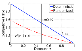
Figure 2: Competitive ratios of both deterministic and randomized algorithms.

We visualize in Fig. 2 the competitive ratios of both deterministic and randomized algorithms against the hourly discount $\alpha$ offered by reserved instances. Compared with the deterministic algorithm, we see that introducing randomness significantly improves the competitive ratio in all cases. The two algorithms become exactly the same when $\alpha=1$, at which the reservation offers no discount and will never be considered. In particular, when it comes to Amazon EC2 with reservation discount $\alpha=0.49$ (standard 1-year reservation, light utilization), the randomized algorithm leads to a competitive ratio of 1.23, compared with the 1.51-competitiveness of the deterministic alternative. Yet, this does not imply that the former always incurs less instance acquiring costs — it is more efficient than the deterministic alternative only in expectation.

VI Cost Management with Short-Term Demand Predictions

In the previous sections, our discussions focus on the extreme cases, with either full future demand information (i.e., the offline case in Sec. III) or no a priori knowledge of the future (i.e., the online case in Sec. IV and V). In this section, we consider the middle ground in which short-term demand predictions are reliable. For example, websites typically see diurnal patterns exhibited on their workloads, based on which it is possible to have a demand prediction window that is weeks into the future. Both our online algorithms can be easily extended to utilize these knowledge of future demands when making reservation decisions.

We begin by formulating the instance reservation problem with limited information of future demands. Let $w$ be the prediction window. That is, at any time $t$, a user can predict its future demands $d_{t+1},\dots,d_{t+w}$ in the next $w$ hours. Since only short-term predictions are reliable, one can safely assume that the prediction window is less than a reservation period, i.e., $w<\tau$. The instance reservation problem resembles the online reservation problem (1), except that the instance purchase decisions made at each time $t$, i.e., the number of reserved instances ($r_{t}$) and on-demand instances ($o_{t}$), are based on both history and future demands predicted, i.e., $d_{1},\dots,d_{t+w}$. The competitive analysis (Definition 1) remains valid in this case.

The Deterministic Algorithm: We extend our deterministic online algorithm as follows. As before, all workloads are by default served by on-demand instances. At time $t$, we can predict the demands up to time $t+w$. Unlike the online deterministic algorithm, we check the use of on-demand instances in a reservation period across both history and future, starting from time $t+w-\tau+1$ to $t+w$. A new instance is reserved at time $t$ whenever we see an on-demand instance incurring more costs than the break-even point $\beta$ and the currently effective reservations are less than the current demand $d_{t}$. Algorithm 3, also denoted by $A_{\beta}^{w}$, shows the details.

Algorithm 3 Deterministic Algorithm $A_{\beta}^{w}$ with Prediction Window $w$

1.  Let $x_{i}$ be the number of reserved instances at time $i$, Initially, $x_{i}\leftarrow 0$ for all $i=0,1,\dots$

2.  Upon the arrival of demand $d_{t}$, loop as follows:

3.  while $p\sum_{i=t+w-\tau+1}^{t+w}I(d_{i}>x_{i})>\beta$ and $x_{t}<d_{t}$ do

4.     Reserve a new instance: $r_{t}\leftarrow r_{t}+1$.

5.     Update the number of reservations that can be used in the future: $x_{i}\leftarrow x_{i}+1$ for $i=t,\dots,t+\tau-1$.

6.     Add a “phantom” reservation to the history, indicating that the history has already been “processed”: $x_{i}\leftarrow x_{i}+1$ for $i=t+w-\tau+1,\dots,t-1$.

7.  end while

8.  Launch on-demand instances: $o_{t}\leftarrow(d_{t}-x_{t})^{+}$.

9.  $t\leftarrow t+1$, repeat from 2.

The Randomized Algorithm: The randomized algorithm can also be constructed as a random distribution over a family of deterministic algorithms similar to $A_{\beta}^{w}$. In particular, let $A_{z}^{w}$ be similarly defined as algorithm $A_{\beta}^{w}$ with $\beta$ replaced by $z\in[0,\beta]$ in line 3 of Algorithm 3. The value of $z$ reflects the aggressiveness of instance reservation. The smaller the $z$, the more aggressive the reservation strategy. Similar to the online randomized, we introduce randomness to strike a good balance between reserving aggressively and conservatively. Our algorithm randomly picks $z\in[0,\beta]$ according to the same density function $f(z)$ defined by (24), and runs the resulting algorithm $A_{z}^{w}$. Algorithm 4 formalizes the description above.

Algorithm 4 Randomized Algorithm with Prediction Window $w$

1.  Randomly pick $z\in[0,\beta]$ according to a density function $f(z)$ defined by (24)

2.  Run $A_{z}^{w}$

It is easy to see that both the deterministic and the randomized algorithms presented above improve the cost performance of their online counterparts, due to the knowledge of future demands. Therefore, we have Proposition 5 below. We will quantify their performance gains via trace-driven simulations in the next section.

Proposition 5

Algorithm 3 is $(2-\alpha)$-competitive, and Algorithm 4 is $e/(e-1+\alpha)$-competitive.

VII Trace-Driven Simulations

So far, we have analyzed the cost performance of the proposed algorithms in a view of competitive analysis. In this section, we evaluate their performance for practical cloud users via simulations driven by a large volume of real-world traces.

VII-A Dataset Description and Preprocessing

Long-term user demand data in public IaaS clouds are often confidential: no cloud provider has released such information so far. For this reason, we turn to Google cluster-usage traces that were recently released in [16]. Although Google is not a public IaaS cloud, its cluster-usage traces record the computing demands of its cloud services and Google engineers, which can represent the computing demands of IaaS users to some degree. The dataset contains 40 GB of workload resource requirements (e.g., CPU, memory, disk, etc.) of 933 users over 29 days in May 2011, on a cluster of more than 11K Google machines.

Demand Curve: Given the workload traces of each user, we ask the question: How many computing instances would this user require if it were to run the same workload in a public IaaS cloud? For simplicity, we set an instance to have the same computing capacity as a cluster machine, which enables us to accurately estimate the run time of computational tasks by learning from the original traces. We then schedule these tasks onto instances with sufficient resources to accommodate their requirements. Computational tasks that cannot run on the same server in the traces (e.g., tasks of MapReduce) are scheduled to different instances. In the end, we obtain a demand curve for each user, indicating how many instances this user requires in each hour. Fig. 3 illustrates such a demand curve for a user.

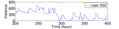
Figure 3: The demand curve of User 552 in Google cluster-usage traces [16], over 1 month.

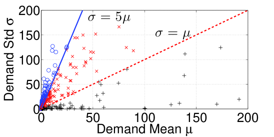
Figure 4: User demand statistics and group division.

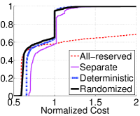
(a) Cost CDF (all users)

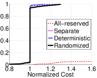
(b) Cost CDF (high fluctuation)

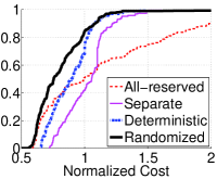
(c) Cost CDF (medium fluctuation)

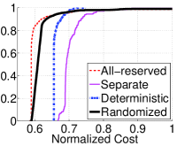
(d) Cost CDF (stable demands)

Figure 5: Cost performance of online algorithms without a priori knowledge of future demands. All costs are normalized to All-on-demand.

User Classification: To investigate how our online algorithms perform under different demand patterns, we classify all 933 users into three groups by the demand fluctuation level measured as the ratio between the standard deviation $\sigma$ and the mean $\mu$.

Specifically, Group 1 consists of users whose demands are highly fluctuating, with $\sigma/\mu\geq 5$. As shown in Fig. 4 (circle ‘o’), these demands usually have small means, which implies that they are highly sporadic and are best served with on-demand instances. Group 2 includes users whose demands are less fluctuating, with $1\leq\sigma/\mu<5$. As shown in Fig. 4 (cross ‘x’), these demands cannot be simply served by on-demand or reserved instances alone. Group 3 includes all remaining users with relatively stable demands ($0\leq\sigma/\mu<1$). As shown in Fig. 4 (plus ‘+’), these demands have large means and are best served with reserved instances. Our evaluations are carried out for each user group.

Pricing: Throughout the simulation, we adopt the pricing of Amazon EC2 standard small instances with the on-demand rate $0.08, the reservation fee $69, and the discount rate $0.039 (Linux, US East, 1-year light utilization). Since the Google traces only span one month, we proportionally shorten the on-demand billing cycle from one hour to one minute, and the reservation period from 1 year to 6 days (i.e., $24\times 365=8760\mbox{ minutes}=6\mbox{ days}$) as well.

VII-B Evaluations of Online Algorithms

We start by evaluating the performance of online algorithms without any a priori knowledge of user demands.

Benchmark Online Algorithms: We compare our online deterministic and randomized algorithms with three benchmark online strategies. The first is All-on-demand, in which a user never reserves and operates all workloads with on-demand instances. This algorithm, though simple, is the most common strategy in practice, especially for those users with time-varying workloads [11]. The second algorithm is All-reserved, in which all computational demands are served via reservations. The third online algorithm is the simple extension to the Bahncard algorithm proposed in [19] (see Sec. II-D), and is referred to as Separate because instances are reserved separately. All three benchmark algorithms, as well as the two proposed online algorithms, are carried out for each user in the Google traces. All the incurred costs are normalized to All-on-demand.

Cost Performance: We present the simulation results in Fig. 5, where the CDF of the normalized costs are given, grouped by users with different demand fluctuation levels. We see in Fig. 5a that when applied to all 933 users, both the deterministic and randomized online algorithms realize significant cost savings compared with all three benchmarks. In particular, when switching from All-on-demand to the proposed online algorithms, more than 60% users cut their costs. About 50% users save more than 40%. Only 2% incur slightly more costs than before. For users who switch from All-reserved to our randomized online algorithms, the improvement is even more substantial. As shown in Fig. 5a, cost savings are almost guaranteed, with 30% users saving more than 50%. We also note that Separate, though generally outperforms All-on-demand and All-reserved, incurs more costs than our online algorithms, mainly due to its ignorance of reservation correlations.

We next compare the cost performance of all five algorithms at different demand fluctuation levels. As expected, when it comes to the extreme cases, All-on-demand is the best fit for Group 1 users whose demands are known to be highly busty and sporadic (Fig. 5b), while All-reserved incurs the least cost for Group 3 users with stable workloads (Fig. 5d). These two groups of users, should they know their demand patterns, would have the least incentive to adopt advanced instance reserving strategies, as naively switching to one option is already optimal. However, even in these extreme cases, our online algorithms, especially the randomized one, remain highly competitive, incurring only slightly higher cost.

However, the acquisition of instances is not always a black-and-white choice between All-on-demand and All-reserved. As we observe from Fig. 5c, for Group 2 users, a more intelligent reservation strategy is essential, since naive algorithms, either All-on-demand or All-reserved, are always highly risky and can easily result in skyrocketing cost. Our online algorithms, on the other hand, become the best choices in this case, outperforming all three benchmark algorithms by a significant margin.

Table II summarizes the average cost performance for each user group. We see that, in all cases, our online algorithms remain highly competitive, incurring near-optimal costs for a user.

TABLE II: Average cost performance (normalized to All-on-demand).

Algorithm	All users	Group 1	Group 2	Group 3
All-reserved	16.48	48.99	1.25	0.61
Separate	0.88	1.01	1.02	0.71
Deterministic	0.81	1.00	0.89	0.67
Randomized	0.76	1.02	0.79	0.63

VII-C The Value of Short-Term Predictions

While our online algorithms perform sufficiently well without knowledge of future demands, we show in this section that more cost savings are realized by their extensions when short-term demand predictions are reliable. In particular, we consider three prediction windows that are 1, 2, and 3 months into the future, respectively. For each prediction window, we run both the deterministic and randomized extensions (i.e., Algorithm 3 and 4) for each Google user in the traces, and compare their costs with those incurred by the online counterparts without future knowledge (i.e., Algorithm 1 and 2). Figs. 6 and 7 illustrate the simulation results, where all costs are normalized to Algorithm 1 and 2, respectively.

As expected, the more information we know about the future demands (i.e., longer prediction window), the better the cost performance. Yet, the marginal benefits of having long-term predictions are diminishing. As shown in Figs. 6a and 7a, long prediction windows will not see proportional performance gains. This is especially the case for the randomized algorithm, in which knowing the 2-month future demand a priori is no different from knowing 3 months beforehand.

Also, we can see in Fig. 6b that for the deterministic algorithm, having future information only benefits those users whose demands are stable or with medium fluctuation. This is because the deterministic online algorithm is almost optimal for users with highly fluctuating demands (see Fig. 5b), leaving no space for further improvements. On the other hand, we see in Fig. 7b that the benefits of knowing future demands are consistent for all users with the randomized algorithm.

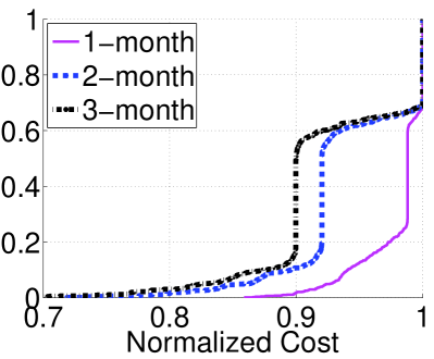
(a) Cost CDF

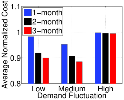
(b) Average cost in different user groups

Figure 6: Cost performance of the deterministic algorithm with various prediction windows. All costs are normalized to the online deterministic algorithm (Algorithm 1) without any future information.

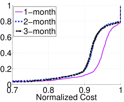
(a) Cost CDF

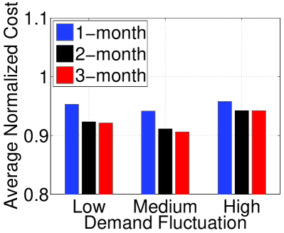
(b) Average cost in different user groups

Figure 7: Cost performance of the randomized algorithm with various prediction windows. All costs are normalized to the online randomized algorithm (Algorithm 1) without any future information.

VIII Related Work

On-demand and reserved instances are the two most prominent pricing options that are widely supported in leading IaaS clouds [3, 4, 5]. Many case studies [11] show that effectively combining the use of the two instances leads to a significant cost reduction.

There exist some works in the literature, including both algorithm design [6, 7, 23] and prototype implementation [8], focusing on combining the two instance options in a cost efficient manner. All these works assume, either explicitly or implicitly, that workloads are statistically stationary in the long-term future and can be accurately predicted a priori. However, it has been observed that in real production applications, ranging from enterprise applications to large e-commerce sites, workload is highly variable and statistically non-stationary [9, 10]. Furthermore, most workload prediction schemes, e.g., [24, 25, 26], are only suitable for predictions over a very short term (from half an hour to several hours). Such limitation is also shared by general predicting techniques, such as ARMA [27] and GARCH models [28]. Some long-term workload prediction schemes [29, 30], on the other hand, are reliable only when demand patterns are easy to recognize with some clear trends. Even in this case, the prediction window is at most days or weeks into the future [29], which is far shorter than the typical span of a reservation period (at least one year in Amazon EC2 [3]). All these factors significantly limit the practical use of existing works.

Our online strategies are tied to the online algorithm literature [18]. Specifically, our instance reservation problem captures a class of rent-or-buy problems, including the ski rental problem [21], the Bahncard problem [19], and the TCP acknowledgment problem [20], as special cases when a user demands no more than one instance at a time. In these problems, a customer obtains a single item either by paying a repeating cost (renting) per usage or by paying a one-time cost (buying) to eliminate the repeating cost. A customer makes one-dimensional decisions only on the timing of buying. Our problem is more complicated as a user demands multiple instances at a time and makes two-dimensional decisions on both the timing and quantity of its reservation. A similar “multi-item rent-or-buy” problem has also been investigated in [22], where a dynamic server provisioning problem is considered and an online algorithm is designed to dynamically turn on/off servers to serve time-varying workloads with a minimum energy cost. It is shown in [22] that, by dispatching jobs to servers that are idle or off the most recently, the problem reduces to a set of independent ski rental problems. Our problem does not have such a separability structure and cannot be equivalently decomposed into independent single-instance reservation (Bahncard) problems, mainly due to the possibility of time multiplexing multiple jobs on the same reserved instance. It is for this reason that the problem is challenging to solve even in the offline setting.

Besides instance reservation, online algorithms have also been applied to reduce the cost of running a file system in the cloud. The recent work [31] introduces a constrained ski-rental problem with extra information of query arrivals (the first or second moment of the distribution), proposing new online algorithms to achieve improved competitive ratios. [31] is orthogonal to our work as it takes advantage of additional demand information to make rent-or-buy decisions for a single item.

IX Concluding Remarks and Future Work

Acquiring instances at the cost-optimal commitment level for time-varying workloads is critical for cost management to lower IaaS service costs. In particular, when should a user reserve instances, and how many instances should it reserve? Unlike existing reservation strategies that require knowledge of the long-term future demands, we propose two online algorithms, one deterministic and another randomized, that dynamically reserve instances without knowledge of the future demands. We show that our online algorithms incur near-optimal costs with the best possible competitive ratios, i.e., $2-\alpha$ for the deterministic algorithm and $e/(e-1+\alpha)$ for the randomized algorithm. Both online algorithms can also be easily extended to cases when short-term predictions are reliable. Large-scale simulations driven by 40 GB Google cluster-usage traces further indicate that significant cost savings are derived from our online algorithms and their extensions, under the prevalent Amazon EC2 pricing.

One of the issues that we have not discussed in this paper is the combination of different types of reserved instances with different reservation periods and utilization levels. For example, Amazon EC2 offers 1-year and 3-year reserved instances with light, medium, and high utilizations. Effectively combining these reserved instances with on-demand instances could further reduce instance acquisition costs. We note that when a user demands no more than one instance at a time and the reservation period is infinite, the problem reduces to Multislope Ski Rental [32]. However, it remains unclear if and how the results obtained for Multislope Ski Rental could be extended to instance acquisition with multiple reservation options.

Appendix A Proof of Lemma 2

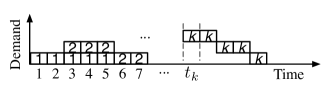
Figure 8: A reservation can be pictorially represented as a reservation strip. For example, reservation 2 is represented as $(2,2,2,1,1)$ with $t_{2}=3$.

We first present a general description for a reserved instance, based on which we reveal the connections between reservations in $A_{\beta}$ and OPT.

Suppose an algorithm reserves $n$ instances 1, 2, …, $n$ at time $t_{1}\leq t_{2}\leq\dots\leq t_{n}$, respectively. Also suppose at time $t$, the active reservations are $i,i+1,\dots,j$. Let demand $d_{t}$ be divided into levels, with level 1 being the bottom. Without loss of generality, we can serve demand at level 1 with reservation $i$, and level 2 with $i+1$, and so on. This gives us a way to describe the use of a reserved instance to serve demands. Specifically, the reservation $k$ is active from $t_{k}$ to $t_{k}+\tau-1$ and is described as a $\tau$-tuple $(l_{t_{k}}^{k},l_{t_{k}+1}^{k},\dots,l_{t_{k}+\tau-1}^{k})$, where $l_{t}^{k}$ is the demand level that $k$ will serve at time $t=t_{k},\dots,t_{k}+\tau-1$. Such a tuple can be pictorially represented as a reservation strip and is depicted in Fig. 8.

We next define a decision strip for every reserved instance in $A_{\beta}$ and will show its connections to the reservation strips in OPT. Suppose an instance is reserved at time $t$ in $A_{\beta}$, leading $x_{i}$’s to update in line 6 and 7 of Algorithm 1. We refer to the bottom figure of Fig. 1 and define the decision strip for this reservation as the region between the original $x$ curve (the solid line) and the newly updated one (the dotted line). Fig. 9 plots the result, where the shaded area is derived from the top figure of Fig. 1. Such a decision strip captures critical information of a reserved instance in $A_{\beta}$. As shown in Fig. 9, the first $\tau$ times of the strip, referred to as the pre-reservation part, reveal the reason that causes this reservation: serving the shaded area on demand incurs more costs than the break-even point $\beta$. The last $\tau$ times are exactly the reservation strip of this reserved instance in $A_{\beta}$, telling how it will be used to serve demands. We therefore denote a decision strip of a reservation $k$ as a $(2\tau-1)$-tuple $\mathbf{l}_{k}=(l_{t_{k}-\tau+1}^{k},\dots,l_{t_{k}}^{k},\dots,l_{t_{k}+\tau-1}^{k})$, where $l_{t}^{k}$ is the demand level of strip $k$ at time $t=t_{k}-\tau+1,\dots,t_{k}+\tau-1$. The pre-reservation part is $(l_{t_{k}-\tau+1}^{k},\dots,l_{t_{k}}^{k})$, while the reservation strip is $(l_{t_{k}}^{k},\dots,l_{t_{k}+\tau-1}^{k})$.

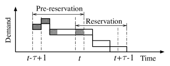
Figure 9: Illustration of a decision strip for a reserved instance in Fig. 1.

We now show the relationship between decision strips of $A_{\beta}$ and reservation strips of OPT. Given the demand sequence, Algorithm $A_{\beta}$ makes $n_{\beta}$ reservations, each corresponding to a decision strip. OPT reserves $n_{\mathrm{OPT}}$ instances, each represented as a reservation strip. We say a decision strip of $A_{\beta}$ intersects a reservation strip of OPT if the two strips share a common area when depicted. The following lemma establishes their connections.

Lemma 4

A decision strip of $A_{\beta}$ intersects at least a reservation strip of OPT.

Proof: We prove by contradiction. Suppose there exists a decision strip of $A_{\beta}$ that intersects no reservation strip of OPT. In this case, the demand in the pre-reservation part (the shaded area in Fig. 9) are served on demand in OPT, incurring a cost more than the break-even point (by the definition of $A_{\beta}$). This implies that the cost of OPT can be further lowered by serving these pre-reservation demands (the shaded area) with a reserved instance, contradicting the definition of OPT.     ∎

Corollary 1

Any two decision strips of $A_{\beta}$ intersect at least two reservation strips of OPT, one for each.

Proof: We prove by contradiction. Suppose there exist two decision strips of $A_{\beta}$, one corresponding to reservation $i$ made at time $t_{i}$ and another to reservation $j$ made at $t_{j}$, $i<j$, that intersect only one reservation strip of OPT. (By Lemma 4, any two decision strips must intersect at least one reservation strip of OPT.) By the analyses of Lemma 4, the reservation strip of OPT intersects the pre-reservation parts of both decision strip $i$ and $j$. It suffices to consider the following two cases.

Case 1: Strip $i$ and $j$ do not overlap in time, i.e., $t_{i}+\tau-1<t_{j}-\tau+1$. As shown in Fig. 10a, having a reservation strip of OPT intersecting the pre-reservation parts of both $i$ and $j$ requires a reservation period that is longer than $\tau$, which is impossible.

Case 2: Strip $i$ and $j$ overlap in time. In this case, the reservation strip of OPT only intersects strip $i$. To see this, we refer to Fig. 10b. Because $i<j$, strip $i$ is depicted below $j$, i.e., $l_{t}^{i}<l_{t}^{j}$ for all $t$ in the overlap. Suppose the reservation strip of OPT intersects decision strip $j$ at time $t$. Clearly, $t$ must be in the overlap and $l_{t}^{i}<l_{t}^{j}$. This implies that at time $t$ in OPT, OPT serves the demand at a lower level $l_{t}^{i}$ by an on-demand instance while serving a higher level $l_{t}^{j}$ via a reservation, which contradicts the definition of the reservation strip.     ∎

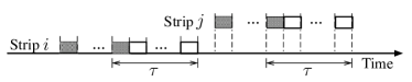
(a) Strip $i$ and $j$ do not overlap in time.

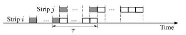
(b) Strip $i$ and $j$ overlap in time.

Figure 10: Two cases of strip $i$ and $j$. They either overlap in time or not.

With Lemma 4 and Corollary 1, we see that the $n_{\beta}$ decision strips of $A_{\beta}$ intersect at least $n_{\beta}$ reservation strips of OPT, indicating that $n_{\beta}\leq n_{\mathrm{OPT}}$.

Appendix B Proof Sketch of Lemma 3

Statement 1: Following the notations used in the proof of Proposition 1, let $S$ be the total costs of demands when priced at the on-demand rate, and $\mathrm{Od}(A_{z})$ be the on-demand costs incurred by algorithm $A_{z}$. It is easy to see

$$\left\{\begin{array}[]{lcl}C_{A_{z}}&=&n_{z}+(1-\alpha)\mathrm{Od}(A_{z})+\alpha S;\\ C_{\mathrm{OPT}}&=&n_{\mathrm{OPT}}+(1-\alpha)\mathrm{Od}(\mathrm{OPT})+\alpha S.\end{array}\right.$$ (34)

Plugging (34) into (26), we see that it is equivalent to proving

$$\mathrm{Od}(A_{z})\leq\mathrm{Od}(\mathrm{OPT})+zn_{\mathrm{OPT}}-E_{z}~{}.$$ (35)

Denote by $\mathrm{Od}(A_{z}\backslash\mathrm{OPT}):=\sum_{t=1}^{T}(o_{z,t}-o_{t}^{*})^{+}p$ the on-demand costs incurred by $A_{z}$ that are not incurred by OPT. With similar arguments as we made for (15), we see $\mathrm{Od}(A_{z}\backslash\mathrm{OPT})\leq zn_{\mathrm{OPT}}$. We therefore derive

$$\mathrm{Od}(A_{z}) =\mathrm{Od}(\mathrm{OPT})+\mathrm{Od}(A_{z}\backslash\mathrm{OPT})-E_{z}$$

$$\leq\mathrm{Od}(\mathrm{OPT})+zn_{\mathrm{OPT}}-E_{z}~{},$$

which is exactly (35).     ∎

Statement 2: For any given demands $\{d_{t}\}$, let $L(n,z)$ be the minimum, over all purchase decisions $D=\{r_{t},o_{t}\}$ with $n$ reserved instances, of the on-demand cost that has been incurred in $D$ but has not been incurred in $A_{z}$, i.e.,

$$\begin{split}L(n,z)&:=\mbox{$\inf_{\{r_{t},o_{t}\}}\sum_{t=1}^{T}(o_{t}-o_{z,t})^{+}p$}\\ \mbox{s.t.}&\quad\mbox{$\sum_{t=1}^{T}r_{t}=n$,}\\ &\quad\mbox{$o_{t}+\sum_{i=t-\tau+1}^{t}r_{i}\geq d_{t}$,}\\ &\quad\mbox{$o_{t},r_{t}\in\{0,1,2,\dots\}$, $t=1,\dots,T$.}\end{split}$$ (36)

We show that for any $u>v\geq z$,

$$L(n_{u},z)\geq(v-z)(n_{v}-n_{u})+L(n_{v},z)~{}.$$ (37)

To see this, let $D_{u}=\{r_{u,t},o_{u,t}\}$ be the purchase decision that leads to $L(n_{u},z)$ and define decision strips for $A_{v}$ and reservation strips for $D_{u}$ similarly as we did in Appendix A. With similar arguments of Corollary 1, we see that a reservation strip of $D_{u}$ intersects at most one decision strip of $A_{v}$. As a result, among all $n_{v}$ decision strips of $A_{v}$, there are at least $n_{v}-n_{u}$ ones that do not intersect any reservation strips of $D_{u}$. We arbitrarily choose $n_{v}-n_{u}$ such decision strips and denote their collections as $B$. Each of these decision strips contains a pre-reservation part with an on-demand cost $v$, of which at most $z$ is also incurred on demand in $A_{z}$ (by definition of $A_{z}$). As a result, an on-demand cost of at least $(v-z)(n_{v}-n_{u})$ is incurred in both $D_{u}$ and $A_{v}$ that is not incurred in $A_{z}$, i.e.,

$$\sum_{t=1}^{T}(\min\{o_{v,t},o_{u,t}\}-o_{z,t})^{+}p\geq(v-z)(n_{v}-n_{u})~{},$$ (38)

where $o_{v,t}$ is the number of on-demand instances launched by $A_{v}$ at time $t$. We now reserve a new instance at the starting time of each decision strip in $B$. Adding to the existing reservations made by $D_{u}$, we have $D^{\prime}=D_{u}\cup B$ as new reserving decisions with $n_{v}$ reserved instances (because $|B|=n_{v}-n_{u}$). Therefore

$$L(n_{u},z) =\mathrm{Od}(D_{u}\backslash A_{z})$$

$$\geq\mathrm{Od}(D^{\prime}\backslash A_{z})+(v-z)(n_{v}-n_{u})$$

$$\geq L(n_{v},z)+(v-z)(n_{v}-n_{u})~{},$$ (39)

where the second inequality holds due to the definition of $L(n_{v},z)$ and the fact that $D^{\prime}$ consists of $n_{v}$ reserved instances.

The rest of the proof follows the framework of [20]. Taking $u=v+\mathrm{d}v$ and integrating from $z$ to $w$, for any $z<w\leq\beta$, we have

$$L(n_{w},z)-L(n_{z},z)\geq\int_{z}^{w}n_{v}\mathrm{d}v-(w-z)n_{w}~{}.$$ (40)

Observing that $L(n_{z},z)=0$, and that $n_{v}\leq n_{w}$ for $v>w$, we have

$$L(n_{w},z)\geq\int_{z}^{\beta}n_{v}\mathrm{d}v-(\beta-z)n_{w}~{}.$$ (41)

Taking $n_{w}=n_{\mathrm{OPT}}$ and noting that $E_{z}\geq L(n_{\mathrm{OPT}},z)$ yields the statement.     ∎

Statement 3: By (34) and noting that $\mathrm{Od}(\mathrm{OPT})\geq E_{z}$, we have

$$C_{\mathrm{OPT}} \geq n_{\mathrm{OPT}}+\alpha S+(1-\alpha)E_{z}$$

$$\geq n_{\mathrm{OPT}}+E_{z}~{},$$ (42)

where the second inequality is derived by noting $S\geq E_{z}$. Letting $z\to 0$ and plugging (27) establishes the statement.     ∎

References

- [1] “Gartner Says Worldwide Cloud Services Market to Surpass $109 Billion in 2012,” https://www.gartner.com/it/page.jsp?id=2163616.
- [2] “The Future of Cloud Adoption,” http://cloudtimes.org/2012/07/14/the-future-of-cloud-adoption/.
- [3] Amazon EC2 Pricing, http://aws.amazon.com/ec2/pricing/.
- [4] ElasticHosts, http://www.elastichosts.com/.
- [5] GoGrid Cloud Hosting, http://www.gogrid.com.
- [6] Y. Hong, M. Thottethodi, and J. Xue, “Dynamic server provisioning to minimize cost in an IaaS cloud,” in Proc. ACM SIGMETRICS, 2011.
- [7] C. Bodenstein, M. Hedwig, and D. Neumann, “Strategic decision support for smart-leasing Infrastructure-as-a-Service,” in Proc. 32nd Intl. Conf. on Info. Sys. (ICIS), 2011.
- [8] K. Vermeersch, “A broker for cost-efficient qos aware resource allocation in EC2,” Master’s thesis, University of Antwerp, 2011.
- [9] C. Stewart, T. Kelly, and A. Zhang, “Exploiting nonstationarity for performance prediction,” ACM SIGOPS Operating Systems Review, vol. 41, no. 3, pp. 31–44, 2007.
- [10] R. Singh, U. Sharma, E. Cecchet, and P. Shenoy, “Autonomic mix-aware provisioning for non-stationary data center workloads,” in Proc. IEEE/ACM Intl. Conf. on Autonomic Computing (ICAC), 2010.
- [11] AWS Case studies, http://aws.amazon.com/solutions/case-studies/.
- [12] “Cloudability,” http://cloudability.com.
- [13] “Cloudyn,” http://www.cloudyn.com.
- [14] “Cloud Express by Apptio,” https://www.cloudexpress.com.
- [15] W. Powell, Approximate Dynamic Programming: Solving the curses of dimensionality. John Wiley and Sons, 2011.
- [16] Google Cluster-Usage Traces, http://code.google.com/p/googleclusterdata/.
- [17] “Amazon ElastiCache,” http://cloudability.com.
- [18] A. Borodin and R. El-Yaniv, Online Computation and Competitive Analysis. Cambridge University Press, 1998.
- [19] R. Fleischer, “On the Bahncard problem,” Theoretical Computer Science, vol. 268, no. 1, pp. 161–174, 2001.
- [20] A. Karlin, C. Kenyon, and D. Randall, “Dynamic TCP acknowledgment and other stories about e/(e-1),” Algorithmica, vol. 36, no. 3, pp. 209–224, 2003.
- [21] A. Karlin, M. Manasse, L. McGeoch, and S. Owicki, “Competitive randomized algorithms for nonuniform problems,” Algorithmica, vol. 11, no. 6, pp. 542–571, 1994.
- [22] T. Lu, M. Chen, and L. L. Andrew, “Simple and effective dynamic provisioning for power-proportional data centers,” IEEE Trans. Parallel Distrib. Syst., vol. 24, no. 6, pp. 1611–1171, 2013.
- [23] W. Wang, D. Niu, B. Li, and B. Liang, “Revenue maximization with dynamic auctions in iaas cloud markets,” in Proc. IEEE ICDCS, 2013.
- [24] G. Chen, W. He, J. Liu, S. Nath, L. Rigas, L. Xiao, and F. Zhao, “Energy-aware server provisioning and load dispatching for connection-intensive internet services,” in Proc. USENIX NSDI, 2008.
- [25] B. Guenter, N. Jain, and C. Williams, “Managing cost, performance, and reliability tradeoffs for energy-aware server provisioning,” in Proc. IEEE INFOCOM, 2011.
- [26] Í. Goiri, K. Le, T. D. Nguyen, J. Guitart, J. Torres, and R. Bianchini, “Greenhadoop: leveraging green energy in data-processing frameworks,” in Proc. ACM EuroSys, 2012.
- [27] G. Box, G. Jenkins, and G. Reinsel, Time Series Analysis: Forecasting and Control. Prentice Hall, 1994.
- [28] T. Bollerslev, “Generalized autoregressive conditional heteroskedasticity,” Journal of Econometrics, vol. 31, no. 3, pp. 307–327, 1986.
- [29] B. Urgaonkar, P. Shenoy, A. Chandra, and P. Goyal, “Dynamic provisioning of multi-tier internet applications,” in Proc. IEEE/ACM Intl. Conf. on Autonomic Computing (ICAC), 2005.
- [30] D. Gmach, J. Rolia, L. Cherkasova, and A. Kemper, “Capacity management and demand prediction for next generation data centers,” in Proc. IEEE Intl. Conf. on Web Services (ICWS), 2007.
- [31] A. Khanafer, M. Kodialam, and K. P. N. Puttaswamy, “The constrained ski-rental problem and its application to online cloud cost optimization,” in Proc. IEEE INFOCOM, 2013.
- [32] Z. Lotker, B. Patt-Shamir, D. Rawitz, S. Albers, and P. Weil, “Rent, lease or buy: Randomized algorithms for multislope ski rental,” in Proc. Symp. on Theoretical Aspects of Computer Science (STAC), 2008.