Constraints on porosity and mass loss in O-star winds from modeling of X-ray emission line profile shapes

Abstract

We fit X-ray emission line profiles in high resolution XMM-Newton and Chandra grating spectra of the early O supergiant $\zeta$ Pup with models that include the effects of porosity in the stellar wind. We explore the effects of porosity due to both spherical and flattened clumps. We find that porosity models with flattened clumps oriented parallel to the photosphere provide poor fits to observed line shapes. However, porosity models with isotropic clumps can provide acceptable fits to observed line shapes, but only if the porosity effect is moderate. We quantify the degeneracy between porosity effects from isotropic clumps and the mass-loss rate inferred from the X-ray line shapes, and we show that only modest increases in the mass-loss rate ($\>\vbox{\hbox{$<$\hskip-7.5pt\lower 4.30554pt\hbox{$\sim$}}}\>40\%$) are allowed if moderate porosity effects ($h_{\infty}\>\vbox{\hbox{$<$\hskip-7.5pt\lower 4.30554pt\hbox{$\sim$}}}\>R_{*}$) are assumed to be important. Large porosity lengths, and thus strong porosity effects, are ruled out regardless of assumptions about clump shape. Thus, X-ray mass-loss rate estimates are relatively insensitive to both optically thin and optically thick clumping. This supports the use of X-ray spectroscopy as a mass-loss rate calibration for bright, nearby O stars.

— stars: mass-loss — stars: winds, outflows — X-rays: stars

1. Introduction

Radiatively driven winds in massive stars have been known to be structured and inhomogeneous virtually since their discovery (Morton, 1967), both from an observational and theoretical standpoint (Lucy & Solomon, 1970; Brucato, 1971). The same instability in the radiative driving force that is responsible for the inhomogeneous nature of these winds is also responsible for generating shocks resulting in X-ray emission (Lucy & White, 1980; Owocki et al., 1988; Feldmeier et al., 1997b). Since these phenomena are so intimately related, it is no surprise that the question of the effects of wind inhomogeneities on X-ray radiative transfer has arisen as well.

A good understanding of X-ray line profile formation in massive star winds is of great importance, as the degree of asymmetry in X-ray line profiles can provide an independent diagnostic of stellar mass loss (Cohen et al., 2010). From an observational perspective, the traditional mass-loss rate diagnostics in the optical, radio, and UV bands are easier to use, but all these diagnostics are subject to modeling uncertainties resulting from wind inhomogeneities. H$\alpha$ recombination lines and radio free-free emission are both the result of collisional processes that scale with the square of density, and thus are sensitive to the degree of clumping in the wind. H$\alpha$ emission originates near the stellar photosphere, while radio free-free emission originates farther out in the wind, and each of these measurements depends on the local degree of inhomogeneity (e.g., Puls et al., 2006). UV P Cygni absorption features probe the ion column density in the wind, but the derivation of a mass-loss rate from an ion column density requires accurate knowledge of the ionization balance (Massa et al., 2003; Fullerton et al., 2006). Furthermore, inhomogeneities in the distribution of wind material in line-of-sight velocity complicate the construction of model absorption profiles (Owocki, 2008; Oskinova et al., 2007; Sundqvist et al., 2010, 2011). If X-ray line profiles are demonstrated to be relatively free of systematic effects from wind inhomogeneities, then X-ray spectroscopy may be used to calibrate the effects of inhomogeneities on traditional mass-loss rate diagnostics.

Because X-ray radiative transfer in stellar winds is generally only affected by continuum photoelectric absorption in the cool bulk of the wind, the only possible way for inhomogeneities to have an effect is if the clumps are optically thick in the continuum and have a large interclump mean free path, leading to porosity. On the other hand, optically thin clumps will only affect diagnostics with opacities that scale with the square of the density, and so do not affect X-ray absorption. The goal of this paper is to empirically constrain the potential effect of porosity on X-ray line diagnostics.

Feldmeier et al. (2003) and Oskinova et al. (2004) have developed a formalism for X-ray radiative transfer in a porous stellar wind, focusing on the case of flat clumps oriented parallel to the stellar surface. They find that porous winds can produce significantly more symmetric line profiles for a given mass-loss rate. Since the assumed mass-loss rate also influences the degree of profile asymmetry, the mass-loss rate and degree of porosity might be expected to become degenerate parameters of line profile fitting. This would reduce the utility of X-ray line shapes as mass-loss rate diagnostics, unless some other observational constraints could be placed on porosity lengths.

In Owocki & Cohen (2006) and Sundqvist et al. (2012, hereafter Paper I), we have developed a generalized formalism for X-ray radiative transfer in a clumpy stellar wind. In particular, Paper I gives a unified treatment of spherical and flat clumps, and explores the effects of a distribution of clump scales. Paper I shows that porosity in models with either flat or spherical clumps tends to produce more symmetric line shapes for a given mass-loss rate. However, flat clumps result in profiles with a distinct shape, with a bump arising near line center (the “Venetian blind effect”; e.g., columns 3 and 4 of Figure 3 in Paper I).

Oskinova et al. (2006) have applied their X-ray radiative transfer formalism to the calculation of emission line profiles, and have compared their model to the observed line profiles of four O stars observed with Chandra. They found that a model including porosity from flat clumps could qualitatively reproduce the observed profile shapes. However, they have not formally evaluated the quality of their fits, and have not quantitatively explored the tradeoffs between porosity and mass loss rate.

In this paper, we aim to confront models of X-ray emission line profiles with high quality observational data to evaluate how well porous and non-porous models can explain the X-ray emission of O stars, to evaluate the effects of both flat and spherical clumps, and to quantify the tradeoffs between porosity and mass-loss rate in modeling the observations. We focus on the high quality archival observations of the bright, well-studied O star $\zeta$ Pup, which has been observed by Chandra, as well as by XMM-Newton for nearly one million seconds. In addition to the high quality of the available data, $\zeta$ Pup has the advantage of being a single, non-magnetic O star, and it has visibly asymmetric X-ray line profiles, indicating that absorption of X-rays by the wind is significant and measurable.

This paper is organized as follows. Section 2 briefly recapitulates our X-ray emission line profile models. In § 3 we describe the observations, and our data reduction and fitting procedures. Section 4 gives the results of our line profile modeling. In Section 5 we compare our results to previous work. In Section 6 we discuss our results and give our conclusions.

2. Model

The models used in this paper are described in Owocki & Cohen (2001), with elaborations for porosity in Owocki & Cohen (2006) and Paper I. Here we give a brief recapitulation of these models and a description of their implementation.

The emergent X-ray spectrum from the wind of a massive star is calculated assuming the X-rays are formed in a small fraction of the wind, while the cool bulk of the wind absorbs the X-rays as they propagate through it. The emergent luminosity at a given wavelength $\lambda$ is

$$L_{\lambda}=4\pi\int dV\eta_{\lambda}e^{-\tau}\,,$$ (1)

where the integral is taken over the X-ray emitting volume of the wind, $\eta_{\lambda}$ gives the X-ray emissivity, and $\tau$ is the X-ray optical depth due to bound-free transitions in the cool bulk of the wind, evaluated by an integral along the line of sight. The X-ray emitting volume is typically taken to have a lower radial cutoff $R_{0}$. In most of this work, we assume that there is no upper radial cutoff $R_{\mathrm{max}}$, but in Section 5 we instead assume a finite value for $R_{\mathrm{max}}$in order to compare our work with that of Oskinova et al. (2006).

It is possible to incorporate porosity within the framework of Owocki & Cohen (2001) by making appropriate modifications to the optical depth term in Equation 1. In this paper, we use the implementations of isotropic and anisotropic porosity described in Paper I. The bound-free absorption of an X-ray photon emitted at $z_{\rm e}$ in direction $\hat{z}$ is given by the optical depth

$$\tau=\int_{z_{\rm e}}^{\infty}\chi_{\rm eff}\,dz,$$ (2)

where the effective opacity $\chi_{\rm eff}$ accounts for any porosity. $\chi_{\rm eff}$ is calculated using the “inverse” (or Rosseland) law for bridging the optically thin and optically thick regimes

$$\frac{\chi_{\rm eff}}{\chi}=\frac{1}{1+\tau_{\rm cl}},$$ (3)

where $\chi$ is the atomic opacity per unit length, proportional to the mass-loss rate and here characterized by the fiducial optical depth $\tau_{\star}=\dot{M}\kappa/(4\pi R_{\star}v_{\infty})$, with mass absorption coefficient $\kappa$ and wind terminal speed $v_{\infty}$. The clump optical depth is

$$\tau_{\rm cl}=\chi h/|\mu|,$$ (4)

where $\mu$ is the directional cosine for a photon impacting a clump; isotropic porosity is recovered by replacing $\mu$ with unity (Paper I). Note from Equation (3) that the effective opacity approaches the atomic opacity when $\tau_{\rm cl}\ll 1$. For the porosity length $h$ we assume the “velocity stretch” form $h(r)/h_{\infty}=v(r)/v_{\infty}$, where the velocity field is given by the standard “$\beta$-law” $v(r)/v_{\infty}=(1-R_{\star}/r)^{\beta}$. Thus, to evaluate X-ray line profiles accounting for porosity, it is only necessary to specify one additional parameter beyond $\tau_{*}$ and $R_{0}$: the terminal porosity length $h_{\infty}$.

It is also possible to account for the effects of UV photoexcitation of metastable levels in He-like ions and resonance scattering of strong X-ray lines within this framework (Leutenegger et al., 2006, 2007). Because the focus of this paper is to derive observational constraints on porosity and its effects on mass-loss rate determinations, we do not use fits to He-like triplets for this purpose, since they are blended. However, in our exploration of the effects of a finite upper radial cutoff $R_{\mathrm{max}}$in Section 5, we fit He-like triplet complexes to obtain constraints on $R_{\mathrm{max}}$. Also, with the exception of our fits to He-like complexes, we also do not account for resonance scattering, which might have a moderate effect on derived mass-loss rates, but will not affect our conclusions about the suitability of porous models or the quantitative tradeoff between porosity and mass-loss rate.

All of the models are implemented as local models in the X-ray spectral fitting package XSPEC (Arnaud, 1996). The code is freely available for download and is issued under the General Public License.

3. Observations, data reduction, and model fitting

$\zeta$ Pup was observed by Chandra on 2000 March 28-29 using the High Energy Transmission Grating Spectrometer (HETGS; ObsID 640, 67.7 ks effective exposure time). $\zeta$ Pup was also observed several times in the last $\sim$ 10 years by XMM-Newton, with total effective exposure time in excess of 0.8 Ms; the list of observations used is given in Table 1. The Chandra Medium Energy Grating (MEG), High Energy Grating (HEG), and XMM-Newton Reflection Grating Spectrometer (RGS) spectra are presented in Figure 1.

The HETGS data were reprocessed using CIAO 4.2 and CALDB 4.3.1 in order to apply optimized contemporary charge transfer inefficiency (CTI) calibrations. Standard procedures were used to produce spectra, response matrices, and ancillary response files.

The RGS (den Herder et al., 2001) data were processed using the XMM SAS 11.0.0. rgsproc was used with the following significant modifications from default settings: pixel-by-pixel corrections to CTI based on contemporary diagnostic exposures were applied; periods of high background were rejected; events on CCD node interfaces, near the edges of CCDs, and next to bad pixels were not rejected; “cool” pixels that have been flagged as having consistently high CTI were rejected. The resulting spectra were then coadded using rgscombine.

RGS spectra are affected by small, systematic shifts in the wavelength scale. The shifts are different for each observation, but constant within each observation. The shifts have an rms deviation of $\sigma=8{\mathrm{m\AA}}$ (den Herder et al., 2001). The most recent calibration implements a correction to the RGS boresight which zeroes out the mean systematic wavelength scale shift in the data used for calibration (Coia & Pollock, 2008). Since we have combined a large number of observations of $\zeta$ Pup, the overall systematic wavelength scale shift is reduced, and the combined data set is broadened. For $N$ independent observations of equal length, the systematic shift in the combined data set is expected to be of order $8\mathrm{m\AA}/\sqrt{N}$. Since we are using 18 observations of roughly equal length, we estimate a net systematic uncertainty in the wavelength scale of $\sim$2 mÅ.

Based on the fitting results we report in Section 4, we believe that the corrections to the RGS boresight implemented in the most recent version of the SAS still result in relative differences between the RGS1 and RGS2 wavelength scales of $\sim 3-5$ mÅ. Thus, any quantitative measurement of line profile asymmetry using RGS data will still be dominated by the systematic wavelength scale uncertainty, and joint fits to data from both RGS instruments will have poor fit statistics which are dominated by the systematic disagreement in the relative calibration of these instruments.

Regardless of these systematic uncertainties in the absolute and relative wavelength scales of the RGS instruments, the data are of extremely high statistical quality and are well suited to answering our two key questions: first, do the data show a bump near line center indicating that anisotropic porosity is important?; and second, what is the quantitative tradeoff between porosity effects and mass-loss rate reductions?

We fit the strong emission lines in the HETGS and RGS spectra with the line profile models described in Section 2 using XSPEC 12.6 (Arnaud, 1996). Each line was fit separately, rather than performing a global fit. The continuum was modeled locally for each line using a power law in energy with index 2, which is a good approximation to the shape of the continuum for a small range in energy. For the Chandra data the continuum strength was determined for a given spectral region by direct fitting while excluding all lines. For the RGS data this is not possible because of the extended wings of the instrumental line spread function (LSF), so the continuum strength was fit simultaneously with the line profiles. For lines where data from both RGS and Chandra are usable, we fit them separately and compare results. For lines where data from both RGS instruments is usable, they are fit jointly, using only negative first order data. In all fits to HETGS data, we used only first order data, fitting positive and negative orders simultaneously. We fit MEG and HEG simultaneously, when HEG data were available. When possible, we fit the line over a wavelength range about 20% bigger than the Doppler shift associated with the wind terminal velocity of $v_{\infty}$ = 2250 $\mathrm{km\,s^{-1}}$ (Haser, 1995). When there is a nearby line which could be blended with the line in question, we eliminate part of the wing of the line from the fit, a procedure which has been shown to have little effect on the fit and the derived parameters (Cohen et al., 2010). We explicitly note these cases in our discussion of individual lines at the end of this section.

Closely spaced doublets in the Ly$\alpha$ lines are fit with a single profile model centered at the emissivity-weighted wavelength of the two components.

We assess the goodness of our model fitting and assign confidence limits using the C statistic (Cash, 1979) for the low-background, low-count-per-bin Chandra spectra, and use the chi-square statistic with Churazov weighting (Churazov et al., 1996) for the higher background and higher count RGS data. Confidence limits are assigned using the $\Delta\chi^{2}$ formalism described in Chapter 15.6 of Numerical Recipes (Press et al., 2007). We report formal 68.3% confidence limits throughout this paper, unless otherwise noted.

Because of the systematic wavelength offset between RGS1 and RGS2, the fits to lines where data were available for both RGS instruments usually had $\chi^{2}_{\nu}>2$. This also occurred in some cases where models provided very poor fits to the data. XSPEC deems a model with $\chi^{2}_{\nu}>2$ a poor fit and does not provide confidence intervals for model parameters, so we do not give them in our results for the two lines where even the best-fit models do not provide formally good fits. For models with large porosity lengths, many other lines also do not have formal confidence limits quoted.

Although it is possible to extract meaningful constraints on model parameters from fits to blended lines, we have chosen to focus on a few strong lines with minimal blending in order to emphasize constraints on porosity and quantitative tradeoffs between porosity and mass-loss rate. Thus, we do not include fits to He-like triplets in our study of the effects of porosity, nor do we include the N VII Ly$\alpha$ line, which is blended with N VI He$\beta$.

Below, we give notes on several of the lines which we fit. Also, note that for the RGS there are several lines which show variations in the effective area due to hot pixels (visible as narrow “dips” in both the spectrum and model). These variations are correctly accounted for by the standard RGS calibration data and pipeline processing. We also tested the effect of excluding these bins from our fits, and found that our results did not change significantly.

Mg XII Ly$\alpha$: The RGS has relatively poor resolving power at this wavelength and does not provide strong constraints on profile shape, so we only fit the HETGS data.

Ne X Ly$\alpha$: The Ne X Ly$\alpha$ doublet is blended with a nearby Fe XVII line at 12.124 Å, which has a comparable temperature-dependent emissivity. It is so close in wavelength to the Ne X lines, which are themselves very close together, that the feature can safely be modeled as a single profile. In contrast, there are two additional iron lines — another Fe XVII line at 12.266 Å and an Fe XXI line at 12.284 Å, which forms at higher temperatures — that may be blended with the red wing of the Ne X line. We therefore exclude the longest wavelength portion of this line from our fitting for both the Chandra and XMM-Newton data.

Fe XVII 15.014Å: The RGS data for this line are moderately affected by blending from the wings of neighboring lines, especially the strong Fe XVII line at 15.261Å, so we have excluded the red wing of this line for the RGS data sets. There are also a number of weak lines from the Rydberg series of O VIII in this spectral region, as well as satellite lines from Fe XVI. Neither of these are strong enough to have a significant effect on the profile shape.

Fe XVII 16.780Å: This line is slightly contaminated by the Rydberg series of O VII, but this does not have a significant effect on the line profile shape. We use only the MEG data and not the RGS data, because of contamination from the extended wings of the RGS LSF from the nearby lines at 17.051 and 17.096 Å.

O VIII Ly$\alpha$: There is slight blending with the Rydberg series of N VI, but these lines are sufficiently weak that they do not have a significant effect on the O VIII profile shape. Most of the MEG counts come from the negative first order, which falls on one of the back illuminated ACIS CCD chips, which has much higher detection efficiency.

N VII Ly$\beta$: This line is somewhat weak, but valuable because it is unblended. The Chandra data are too weak to give meaningful constraints. Most of the RGS observations put part of this line on a gap between CCD chips of RGS1, but enough observations exist with small pointing offsets to give acceptable exposure over the whole line. This line falls on a failed CCD of RGS2, so no data are available from that spectrometer.

Table 1List of XMM-Newton Observations of $\zeta$ Pup with Net Exposure Times.

ObsID	Date	Exposure Time (ks)
		RGS1	RGS2
0095810301	2000 Jun 8	52.6	51.0
0095810401	2000 Oct 15	39.9	38.5
0157160401	2002 Nov 10	41.6	40.2
0157160501	2002 Nov 17	38.7	38.7
0157160901	2002 Nov 24	43.5	43.5
0157161101	2002 Dec 15	27.8	27.8
0159360101	2003 May 30	66.3	66.3
0163360101	2003 Dec 6	41.5	41.5
0159360301	2004 Apr 12	27.7	27.7
0159360401	2004 Nov 14	57.3	57.3
0159360501	2005 Apr 16	34.6	34.6
0159360701	2005 Oct 15	23.5	23.4
0159360901	2005 Dec 3	48.3	48.2
0159361101	2006 Apr 17	42.5	42.4
0414400101	2007 Apr 9	58.5	58.5
0159361301	2008 Oct 13	61.2	61.2
0561380101	2009 Nov 3	64.1	64.2
0561380201	2010 Oct 7	76.7	76.7
Total		846.2	841.8

Figure 1.— The extracted coadded positive and negative first order MEG (top panel) and HEG (second panel) spectra along with the negative first order RGS1 (third panel) and RGS2 (bottom panel) spectra (coadded 18 pointings).

4. Results

We fit each line in the XMM-Newton and Chandra grating spectra according to the methodology described in Section 3. As discussed in that section, we exclude from our analysis those lines that are too weak or too blended to provide strong constraints on the parameters of the line profile model, described in Section 2. For those lines that do provide useful results, Tables 2 and 3 summarize the results of the line profile fits that do not include any porosity. Tables 4–7 summarize the results of line profile fits including porosity.

In this section, we give single parameter confidence limits for all parameters of interest. These single parameter confidence limits are determined with all other parameters of interest free. They are evaluated for a change in the fit statistic of 1.0 (68.3% confidence, corresponding to 1-$\sigma$). These confidence limits are based only on the change in fit statistic under variation of model parameters and do not reflect systematic uncertainties.

Table 2Wind profile model without porosity: fit results to the Chandra HETGS spectra

ion	$\lambda$	$\tau_{*}$	$R_{0}$	Normalization	$C$	$N_{\rm bins}$
	(Å)		($R_{*}$)	($10^{-4}$ photons cm-2 s-1)
Mg XII Ly$\alpha$	8.4210	$1.22_{-.44}^{+.78}$	$1.34_{-.21}^{+.17}$	$0.294_{-.022}^{+.024}$	186.5	188
Ne X Ly$\alpha$	12.1339	$2.01_{-.24}^{+.27}$	$1.45_{-.08}^{+.13}$	$2.71_{-.09}^{+.09}$	191.4	176
Fe XVII	15.014	$1.94_{-.33}^{+.32}$	$1.55_{-.12}^{+.12}$	$5.24_{-.17}^{+.24}$	280.8	308
Fe XVII	16.780	$3.01_{-.70}^{+.32}$	$1.01_{-.01}^{+.59}$	$2.45_{-.17}^{+.13}$	174.9	308
O VIII Ly$\alpha$	18.969	$3.00_{-.54}^{+.54}$	$1.22_{-.21}^{+.37}$	$3.70_{-.35}^{+.29}$	150.9	130

Table 3Wind profile model without porosity: fit results to the XMM-Newton RGS spectra

Ion	$\lambda$	$\tau_{*}$	$R_{0}$	Normalization	$\chi^{2}$	$N_{\rm bins}$
	(Å)		($R_{*}$)	($10^{-4}$ photons cm-2 s-1)
Ne X Ly$\alpha$	12.1339	$1.81_{-.22}^{+.25}$	$1.61_{-.18}^{+.15}$	$3.10_{-.08}^{+.08}$	24.0	19
Fe XVII	15.014	$1.77$	$1.57$	$6.39$	129.5	52
O VIII Ly$\alpha$	18.969	$3.14$	$1.01$	$4.66$	204.3	72
N VII Ly$\beta$	20.910	$4.93_{-.97}^{+.66}$	$1.41_{-.40}^{+.62}$	$1.66_{-.10}^{+.07}$	40.5	36

4.1. Comparison of RGS and Chandra Results

We first fit each line without including the effects of porosity. As can be seen by inspecting the $\tau_{*}$ and $R_{0}$ parameters and their confidence limits in Tables 2 and 3, we find very good agreement for the three lines common to both RGS and Chandra datasets. As an illustrative case, Figure 2 shows the fits to the Fe XVII line at 15.014 Å in the RGS and HETGS spectra. The fitted $\tau_{*}$ values are consistent with a mass-loss rate of $\sim 3\times 10^{-6}$ $M_{\odot}\mathrm{yr}^{-1}$ (or a correspondingly lower mass-loss rate if higher wind opacity is adopted), as derived from the ensemble of Chandra HETGS lines in Cohen et al. (2010), and the fitted $R_{0}$ values of $\sim 1.5$ $R_{*}$ are consistent with the predictions of line-driven instability (LDI) simulations of wind shock formation (Feldmeier et al., 1997b; Runacres & Owocki, 2002). The overall agreement between the $\tau_{*}$ values found in lines from these two datasets has recently been confirmed by Nazé et al. (2012).

Figure 2.— The Chandra MEG (left panel) and XMM-Newton RGS1 (right panel) data for the Fe XVII line at 15.014 Å, along with the respective best-fit models. The vertical dashed line in each figure represents the laboratory rest wavelength of the line. The vertical dotted lines denote the Doppler shift associated with the wind terminal velocity of $v_{\infty}=2250\,\mathrm{km\,s^{-1}}$. Although the left panel shows only the MEG data, the HEG data were fit simultaneously. The right panel shows only the RGS1 data; however, both RGS datasets were fit simultaneously. (A color version of this figure is available in the online journal.)

4.2. Constraints on Porosity Models from Individual Lines

The fits presented in the previous subsection show that the simple line-profile model without porosity provides good fits to both the Chandra and XMM-Newton data. The derived parameters are physically reasonable in the context of embedded wind shocks. However, it is possible that models that include the effects of porosity could also fit the data. We now turn our attention to line profile models that include anisotropic or isotropic porosity.

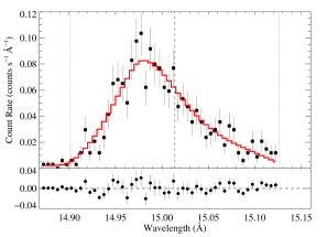
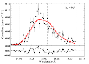
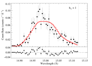
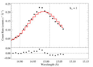
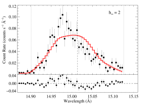
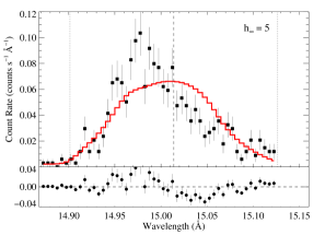
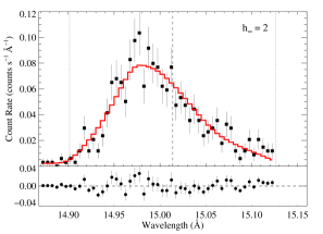
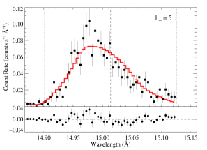
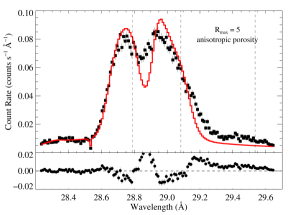
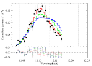
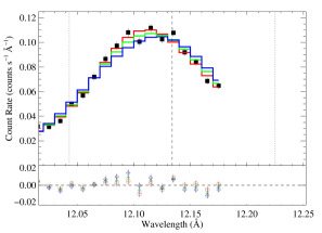
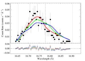
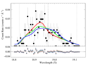
First, we report on the fitting of models that assume anisotropic porosity, from radially oriented, flattened clumps. We first performed fits that allowed the terminal porosity length to be a free parameter. These fits generally prefer $h_{\infty}=0$ (i.e., no porosity, recovering the same results as in Section 4.1). To further explore the effects of anisotropic porosity on the line profiles, we next fit models with fixed values of the terminal porosity length, $h_{\infty}$ = 0.5, 1, 2, and 5 $R_{*}$. We find increasingly poor fits as the value of the terminal porosity length increases. To illustrate these trends, Figure 3 shows the Fe XVII line at 15.014 Å, with the best-fit models assuming each of the four values of $h_{\infty}$. Plots of fits to the other lines in the spectrum of $\zeta$ Pup using anisotropic porosity models are shown in the Appendix.

Figure 3.— The Chandra MEG (left column) and XMM-Newton RGS (right column) measurements of the Fe XVII line at 15.014 Å, identical to the data shown in Figure 2, but with best-fit anisotropic porosity models superimposed. The characteristic “Venetian blind” bump at line center (see Figure 4 of Oskinova et al. (2004) or Figure 3 of Paper I) can be seen in all these models, with the feature getting stronger with increasing $h_{\infty}$. The effect of porosity on the profile shapes can be seen qualitatively even for the models with the smallest porosity lengths, and even with the moderate resolution of the RGS data. These anisotropic porosity profile models do not provide a good fit to the data. (A color version of this figure is available in the online journal.)

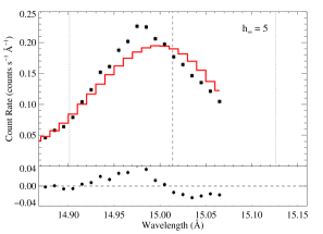Tables 4 and 5 summarize the results of fitting anisotropic porosity models to all of the lines. To facilitate comparison with the non-porous model fitting results, the table repeats those results in the rows with $h_{\infty}=0$. For models that provide very poor fits (i.e. rejected with high probability compared to the best-fitting $h_{\infty}=0$ models), we do not list formal uncertainties on the free model parameters, as the formalism for assigning these uncertainties assumes that the best-fitting models do indeed provide formally good fits.

One clear result that can readily be seen in these tables is that in no case is an anisotropic porous model statistically preferred over the non-porous model. Even for those lines with a lower signal-to-noise ratio, the mildest anisotropic porosity models (with $h_{\infty}=0.5$ $R_{*}$) can be rejected at the 68.3% confidence level.

Table 4Wind profile model with anisotropic porosity: fit results to the Chandra HETGS spectra

ion	$\lambda$	$h_{\infty}$	$\tau_{*}$	$R_{0}$	Normalization	$C$	$N_{\rm bins}$
	(Å)	($R_{*}$)		($R_{*}$)	($10^{-4}$ photons cm-2 s-1)
Mg XII Ly$\alpha$	8.4210	0	$1.22_{-.44}^{+.78}$	$1.34_{-.21}^{+.17}$	$0.294_{-.022}^{+.024}$	186.5	188
		0.5	$1.72_{-.81}^{+.77}$	$1.37_{-.14}^{+.17}$	$0.281_{-.008}^{+.050}$	189.8	188
		1	$1.46_{-.60}^{+1.58}$	$1.45_{-.16}^{+.14}$	$0.305_{-.033}^{+.018}$	191.5	188
		2	$1.83_{-.95}^{+2.08}$	$1.49_{-.12}^{+.13}$	$0.298_{-.024}^{+.023}$	194.1	188
		5	$2.37_{-1.48}^{+6.19}$	$1.54_{-.12}^{+.15}$	$0.297_{-.023}^{+.024}$	198.6	188
Ne X Ly$\alpha$	12.1339	0	$2.01_{-.24}^{+.27}$	$1.45_{-.08}^{+.13}$	$2.71_{-.09}^{+.09}$	191.4	176
		0.5	$2.92_{-.41}^{+.44}$	$1.49_{-.09}^{+.09}$	$2.72_{-.09}^{+.09}$	208.8	176
		1	$3.60_{-.61}^{+.64}$	$1.56_{-.08}^{+.08}$	$2.71_{-.08}^{+.10}$	223.8	176
		2	$5.00_{-1.01}^{+1.37}$	$1.65_{-.09}^{+.07}$	$2.73_{-.09}^{+.10}$	245.0	176
		5	$11.32_{-3.72}^{+5.74}$	$1.77_{-0.10}^{+0.11}$	$2.76_{-0.09}^{+0.10}$	277.6	176
Fe XVII	15.014	0	$1.94_{-.33}^{+.32}$	$1.55_{-.12}^{+.12}$	$5.24_{-.17}^{+.24}$	280.8	308
		0.5	$2.51_{-.40}^{+.68}$	$1.61_{-.14}^{+.08}$	$5.23_{-.18}^{+.23}$	293.9	308
		1	$3.02_{-.65}^{+.84}$	$1.65_{-.10}^{+.10}$	$5.22_{-.18}^{+.23}$	303.8	308
		2	$3.76_{-1.00}^{+1.56}$	$1.74_{-.11}^{+.09}$	$5.22_{-.18}^{+.23}$	317.4	308
		5	$6.95_{-3.01}^{+5.32}$	$1.84_{-.11}^{+.11}$	$5.21_{-.18}^{+.23}$	338.4	308
Fe XVII	16.780	0	$3.01_{-.70}^{+.32}$	$1.01_{-.01}^{+.59}$	$2.45_{-.17}^{+.13}$	174.9	308
		0.5	$4.12_{-.90}^{+.93}$	$1.40_{-.19}^{+.22}$	$2.40_{-.11}^{+.19}$	180.7	308
		1	$5.45_{-1.33}^{+1.46}$	$1.43_{-.09}^{+.25}$	$2.47_{-.18}^{+.13}$	185.6	308
		2	$8.77_{-2.60}^{+3.39}$	$1.58_{-.15}^{+.17}$	$2.41_{-.12}^{+.19}$	193.2	308
		5	$28.99_{-11.96}^{+15.55}$	$1.64_{-.16}^{+.17}$	$2.38_{-.09}^{+.23}$	206.3	308
O VIII Ly$\alpha$	18.969	0	$3.00_{-.54}^{+.54}$	$1.22_{-.21}^{+.37}$	$3.70_{-.35}^{+.29}$	150.9	130
		0.5	$4.26_{-1.16}^{+1.18}$	$1.43_{-.21}^{+.31}$	$3.70_{-.26}^{+.28}$	152.9	130
		1	$5.22_{-1.61}^{+2.17}$	$1.57_{-.23}^{+.26}$	$3.70_{-.27}^{+.30}$	155.1	130
		2	$7.83_{-2.93}^{+3.92}$	$1.66_{-.20}^{+.25}$	$3.62_{-.19}^{+.38}$	158.3	130
		5	$21.10_{-10.50}^{+15.92}$	$1.74_{-.20}^{+.23}$	$3.57_{-.15}^{+.42}$	165.0	130

Table 5Wind profile model with anisotropic porosity: fit results to the XMM-Newton RGS spectra

ion	$\lambda$	$h_{\infty}$	$\tau_{*}$	$R_{0}$	Normalization	$\chi^{2}$	$N_{\rm bins}$
	(Å)	($R_{*}$)		($R_{*}$)	($10^{-4}$ photons cm-2 s-1)
Ne X Ly$\alpha$	12.1339	0	$1.81_{-.22}^{+.25}$	$1.61_{-.18}^{+.15}$	$3.10_{-.08}^{+.08}$	24.0	19
		0.5	$3.92_{-.57}^{+.83}$	$1.35_{-.19}^{+.21}$	$3.18_{-.08}^{+.08}$	27.3	19
		1	$5.71_{-1.00}^{+1.23}$	$1.41_{-.14}^{+.15}$	$3.22_{-.09}^{+.08}$	34.2	19
		2	$12.61$	$1.46$	$3.31$	47.2	19
		5	$64.82$	$1.35$	$3.44$	66.9	19
Fe XVII	15.014	0	$1.77$	$1.57$	$6.39$	129.5	52
		0.5	$3.29$	$1.44$	$6.47$	180.4	52
		1	$4.66$	$1.50$	$6.52$	249.6	52
		2	$8.24$	$1.57$	$6.56$	370.1	52
		5	$35.96$	$1.54$	$6.66$	577.2	52
Fe XVII	16.780	0	$3.38_{-.45}^{+.31}$	$1.54_{-.39}^{+.33}$	$3.01_{-.06}^{+.07}$	30.3	32
		0.5	$4.01_{-.83}^{+.83}$	$1.99_{-.25}^{+.26}$	$3.20_{-.07}^{+.07}$	42.2	32
		1	$4.17_{-1.03}^{+1.26}$	$2.24_{-.25}^{+.24}$	$3.29_{-.07}^{+.08}$	48.0	32
		2	$4.47_{-1.64}^{+1.87}$	$2.49_{-.24}^{+.23}$	$3.41_{-.08}^{+.09}$	54.5	32
		5	$4.28$	$2.89$	$3.59$	62.3	32
O VIII Ly$\alpha$	18.969	0	$3.14$	$1.01$	$4.66$	204.3	72
		0.5	$5.30$	$1.35$	$4.76$	275.2	72
		1	$8.14$	$1.42$	$4.81$	355.1	72
		2	$16.81$	$1.46$	$4.87$	478.8	72
		5	$73.81$	$1.37$	$4.92$	645.8	72
N VII Ly$\beta$	20.910	0	$4.93_{-1.03}^{+.66}$	$1.41_{-.40}^{+.62}$	$1.66_{-.10}^{+.07}$	40.5	36
		0.5	$7.96_{-1.81}^{+2.20}$	$1.60_{-.36}^{+.41}$	$1.69_{-.10}^{+.11}$	52.9	36
		1	$12.95_{-3.34}^{+5.01}$	$1.70_{-.33}^{+.44}$	$1.75_{-.12}^{+.11}$	62.4	36
		2	$34.11$	$1.62$	$1.86$	73.5	36
		5	$>100$	$1.73$	$1.91$	84.4	36

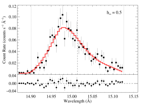
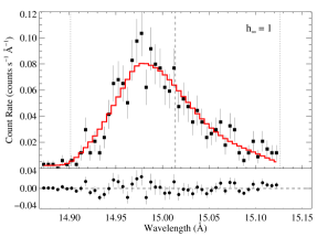
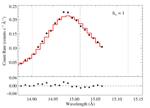
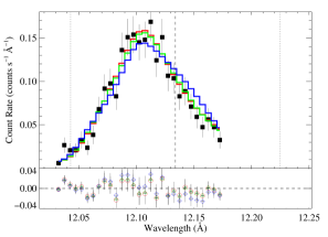
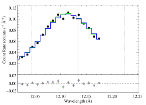
Let us next consider models with isotropic porosity. In this case, there is some degeneracy between porous profiles with lower optical depths and non-porous profiles with higher optical depths, as shown in Figure 3 in Paper I. We find that models with isotropic porosity provide better fits than the corresponding anisotropic porosity profile models. However, when we allow $h_{\infty}$ to be a free parameter, non-porous ($h_{\infty}=0$) models are almost always preferred, and in no case is $h_{\infty}=0$ rejected at greater than 90% confidence for any one line.

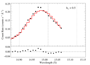
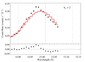
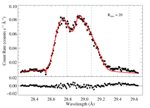
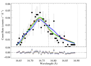
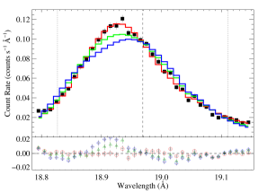
We then fit models with fixed values of terminal porosity length, $h_{\infty}=0.5$, 1, 2, and 5 $R_{*}$. Figure 4 shows fits of the isotropic porosity models to the Fe XVII line at 15.014 Å, and Tables 6 and 7 present fits to all the lines. Plots of fits to the other lines in the spectrum of $\zeta$ Pup using isotropic porosity models are shown in the Appendix.

Figure 5 shows confidence limit contours for the fits to the 15.014 Å line in $\tau_{*}$–$h_{\infty}$ parameter space, illustrating the tradeoff between porosity and wind optical depth. Modest porosity ($h_{\infty}<R_{*}$) is not strongly ruled out, but it does not have a strong effect on $\tau_{*}$, and thus on mass-loss rate estimates from X-ray line profiles.

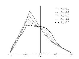
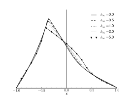
Figure 6 shows the best fit models for the Fe XVII 15.014 Å  line in the Chandra data without accounting for the instrument response. This allows evaluation of the level of degeneracy of $h_{\infty}$ and $\tau_{*}$ in producing roughly comparable line profiles. Even for a small porosity length of $h_{\infty}=0.5R_{*}$, the anisotropic porosity model shows a significant change in shape near line center, with the bump becoming more pronounced for larger porosity lengths. On the other hand, the isotropic porosity models with small $h_{\infty}$ do not look very different from the non-porous model. However, the shape does become increasingly different as porosity length increases. The changes in profile shape support the same conclusions as Figure 5: for isotropic porosity, small porosity lengths can produce similar line shapes that adequately fit the data, while large porosity lengths are ruled out; and for anisotropic porosity, even small porosity lengths change the profile shape so that it does not fit the data.

Figure 4.— The Chandra MEG (left column) and XMM-Newton RGS (right column) measurements of the Fe XVII line at 15.014 Å; identical to the data shown in Figures 2 and 3, but with best-fit isotropic porosity models superimposed. (A color version of this figure is available in the online journal.)

Figure 5.— The 68.3%, 95.4%, and 99.7% confidence limit contours in $\tau_{*}$–$h_{\infty}$ parameter space for the anisotropic (left panel) and isotropic (right panel) porosity model fits to the Fe XVII line at 15.014 Å in the Chandra data. The best fit model is denoted by the filled circle.

Figure 6.— Comparison of the best fit models for the Fe XVII 15.014 Å  line in the Chandra data. The model profile flux is shown as a function of the scaled wavelength $x\equiv(\delta\lambda/\lambda_{0})(c/v_{\infty})$. Anisotropic porosity is shown in the left panel, while isotropic is shown in the right panel. Note that the best fit anisotropic porosity models have a very different shape from the best fit nonporous model because of the enhancement near line center from the “Venetian blind effect”.

Table 6Wind profile model with isotropic porosity: fit results to the Chandra HETGS spectra

Ion	$\lambda$	$h_{\infty}$	$\tau_{*}$	$R_{0}$	Normalization	$C$	$N_{\rm bins}$
	(Å)	($R_{*}$)		($R_{*}$)	($10^{-4}$ photons cm-2 s-1)
Mg XII Ly$\alpha$	8.4210	0	$1.22_{-.44}^{+.78}$	$1.34_{-.21}^{+.17}$	$0.294_{-.022}^{+.024}$	186.5	188
		0.5	$1.31_{-.48}^{+.74}$	$1.38_{-.18}^{+.14}$	$0.300_{-.029}^{+.019}$	186.8	188
		1	$1.46_{-.58}^{+.93}$	$1.39_{-.15}^{+.14}$	$0.300_{-.028}^{+.019}$	187.1	188
		2	$1.79_{-.80}^{+1.42}$	$1.41_{-.12}^{+.14}$	$0.300_{-.028}^{+.020}$	187.7	188
		5	$3.19_{-1.84}^{+4.33}$	$1.47_{-.10}^{+.12}$	$0.301_{-.028}^{+.020}$	189.7	188
Ne X Ly$\alpha$	12.1339	0	$2.01_{-.24}^{+.27}$	$1.45_{-.08}^{+.13}$	$2.71_{-.09}^{+.09}$	191.4	176
		0.5	$2.39_{-.35}^{+.33}$	$1.49_{-.08}^{+.10}$	$2.69_{-.07}^{+.11}$	191.8	176
		1	$2.80_{-.44}^{+.44}$	$1.51_{-.07}^{+.09}$	$2.69_{-.08}^{+.10}$	192.5	176
		2	$3.86_{-.69}^{+.75}$	$1.54_{-.08}^{+.07}$	$2.69_{-.08}^{+.10}$	195.0	176
		5	$9.24_{-2.15}^{+2.82}$	$1.61_{-.06}^{+.08}$	$2.69_{-.09}^{+.09}$	208.5	176
Fe XVII	15.014	0	$1.94_{-.33}^{+.32}$	$1.55_{-.12}^{+.12}$	$5.24_{-.17}^{+.24}$	280.8	308
		0.5	$2.18_{-.39}^{+.42}$	$1.58_{-.10}^{+.11}$	$5.24_{-.17}^{+.24}$	282.0	308
		1	$2.46_{-.47}^{+.54}$	$1.61_{-.13}^{+.08}$	$5.24_{-.17}^{+.24}$	283.4	308
		2	$3.09_{-.66}^{+.89}$	$1.65_{-.09}^{+.08}$	$5.24_{-.18}^{+.24}$	286.4	308
		5	$5.70_{-1.66}^{+2.75}$	$1.74_{-.09}^{+.07}$	$5.23_{-.18}^{+.23}$	297.2	308
Fe XVII	16.780	0	$3.01_{-.70}^{+.32}$	$1.01_{-.01}^{+.59}$	$2.45_{-.17}^{+.13}$	174.9	308
		0.5	$3.59_{-.87}^{+.93}$	$1.35_{-.31}^{+.28}$	$2.39_{-.11}^{+.19}$	174.1	308
		1	$4.38_{-1.06}^{+1.11}$	$1.42_{-.17}^{+.21}$	$2.43_{-.15}^{+.15}$	173.3	308
		2	$6.52_{-1.75}^{+1.99}$	$1.48_{-.11}^{+.17}$	$2.40_{-.12}^{+.19}$	172.6	308
		5	$17.88_{-6.00}^{+6.52}$	$1.60_{-.11}^{+.14}$	$2.43_{-.14}^{+.17}$	176.3	308
O VIII Ly$\alpha$	18.969	0	$3.00_{-.54}^{+.54}$	$1.22_{-.21}^{+.37}$	$3.70_{-.35}^{+.29}$	150.9	130
		0.5	$3.85_{-1.10}^{+1.05}$	$1.32_{-.20}^{+.38}$	$3.70_{-.28}^{+.29}$	150.9	130
		1	$4.42_{-1.47}^{+1.74}$	$1.45_{-.23}^{+.34}$	$3.71_{-.29}^{+.28}$	151.0	130
		2	$5.85_{-2.19}^{+2.88}$	$1.56_{-.19}^{+.28}$	$3.62_{-.19}^{+.37}$	151.1	130
		5	$13.23_{-5.80}^{+8.74}$	$1.69_{-.15}^{+.21}$	$3.60_{-.17}^{+.39}$	152.1	130

Table 7Wind profile model with isotropic porosity: fit results to the XMM-Newton RGS spectra

Ion	$\lambda$	$h_{\infty}$	$\tau_{*}$	$R_{0}$	Normalization	$\chi^{2}$	$N_{\rm bins}$
	(Å)	($R_{*}$)		($R_{*}$)	($10^{-4}$ photons cm-2 s-1)
Ne X Ly$\alpha$	12.1339	0	$1.81_{-.22}^{+.25}$	$1.61_{-.18}^{+.15}$	$3.10_{-.08}^{+.08}$	24.0	19
		0.5	$2.07_{-.27}^{+.34}$	$1.61_{-.16}^{+.15}$	$3.10_{-.08}^{+.08}$	24.0	19
		1	$2.41_{-.34}^{+.45}$	$1.61_{-.15}^{+.15}$	$3.10_{-.08}^{+.09}$	24.1	19
		2	$3.42_{-.61}^{+.87}$	$1.60_{-.13}^{+.14}$	$3.11_{-.09}^{+.08}$	24.2	19
		5	$12.99_{-4.14}^{+6.62}$	$1.58_{-.12}^{+.13}$	$3.16_{-.08}^{+.08}$	26.3	19
Fe XVII	15.014	0	$1.77$	$1.57$	$6.39$	129.5	52
		0.5	$2.02$	$1.58$	$6.40$	131.4	52
		1	$2.33$	$1.59$	$6.40$	133.6	52
		2	$3.23$	$1.60$	$6.40$	139.3	52
		5	$9.96$	$1.61$	$6.44$	175.6	52
Fe XVII	16.780	0	$3.38_{-.45}^{+.31}$	$1.54_{-.39}^{+.33}$	$3.01_{-.06}^{+.07}$	30.3	32
		0.5	$3.94_{-.63}^{+.56}$	$1.65_{-.23}^{+.26}$	$3.01_{-.06}^{+.07}$	31.1	32
		1	$4.50_{-.83}^{+.89}$	$1.73_{-.21}^{+.23}$	$3.03_{-.07}^{+.06}$	32.2	32
		2	$5.61_{-1.17}^{+1.53}$	$1.86_{-.18}^{+.20}$	$3.06_{-.07}^{+.07}$	34.4	32
		5	$8.61_{-2.76}^{+4.30}$	$2.13_{-.18}^{+.19}$	$3.19_{-.08}^{+.07}$	40.4	32
O VIII Ly$\alpha$	18.969	0	$3.14$	$1.01$	$4.66$	204.3	72
		0.5	$3.64$	$1.57$	$4.64$	198.0	72
		1	$4.35$	$1.51$	$4.64$	193.4	72
		2	$6.38$	$1.57$	$4.63$	188.9	72
		5	$20.20$	$1.65$	$4.67$	222.3	72
N VII Ly$\beta$	20.910	0	$4.93_{-1.03}^{+.66}$	$1.41_{-.40}^{+.62}$	$1.66_{-.10}^{+.07}$	40.5	36
		0.5	$6.18_{-1.46}^{+1.89}$	$1.65_{-.51}^{+.46}$	$1.66_{-.10}^{+.10}$	40.6	36
		1	$7.42_{-1.91}^{+2.67}$	$1.79_{-.36}^{+.36}$	$1.66_{-.10}^{+.10}$	41.0	36
		2	$10.16_{-2.76}^{+4.26}$	$1.95_{-.30}^{+.33}$	$1.66_{-.10}^{+.10}$	42.4	36
		5	$26.09_{-7.96}^{+12.44}$	$2.14_{-.29}^{+.38}$	$1.69_{-.09}^{+.10}$	49.0	36

4.3. Effects of porosity on inferred mass-loss rates

In Section 4.2 we have shown for several lines in the spectrum of $\zeta$ Pup that anisotropic porosity models do not fit the data for any significant porosity length, and that isotropic porosity models do not fit for large porosity lengths. However, isotropic porosity models with moderate porosity lengths are formally allowed for some individual lines.

Cohen et al. (2010) have fit the ensemble of measured $\tau_{*}$ values for a non-porous model of $\zeta$ Pup by using the mass-loss rate as an adjustable derived parameter, together with a model wind opacity. We can apply the same technique to the $\tau_{*}$ values measured for different porosity lengths to obtain an estimate of X-ray derived mass-loss rate as a function of assumed porosity length. Together with constraints on the porosity length and geometry, whether from X-ray profile modeling or from other observations, this relation gives a quantitative constraint on the contribution of porosity to uncertainties in mass-loss rates derived from fitting X-ray line profiles.

To this end, it is most instructive to consider not the mass-loss rate itself, but the fractional change in mass-loss rate relative to a non-porous model. The derived mass-loss rate scales linearly with measured $\tau_{*}$, and thus the fractional change in derived mass-loss rate must equal the fractional change in measured $\tau_{*}$. Thus, as a simple way to estimate the fractional change in mass-loss rate, we calculate the fractional change in measured $\tau_{*}$ for the ensemble of lines, for a given assumed porosity length. The estimated mass-loss rate increase for isotropic porosity models is roughly linear in $h_{\infty}$, with $\Delta\dot{M}/\dot{M}\sim 0.4$ for $h_{\infty}=R_{*}$. Large porosity lengths indeed produce large changes in inferred mass-loss rate compared to non-porous models, and anisotropic porosity models have a stronger effect than isotropic models. However, all of the models with strong effects are ruled out by our fit results.

5. Comparison with previous results

One of the main results of Section 4 is that anisotropic porosity models are disfavored, as well as isotropic porosity models with large porosity lengths. This is at odds with the conclusions of Oskinova et al. (2006), who report that anisotropic porosity models provide good fits to the line profiles of several bright O stars observed with Chandra, while non-porous models do not fit their data as well.

We show below that the difference in our findings has its root in a less obvious assumption of both our models and those of Oskinova et al.: the radial upper bound for X-ray emission, $R_{\mathrm{max}}$. Oskinova et al. assume $R_{\mathrm{max}}=5\star$ for $\zeta$ Pup, and as high as $R_{\mathrm{max}}=9R_{*}$ for other stars in their sample. On the other hand, in this paper we have until now assumed $R_{\mathrm{max}}=\infty$.

5.1. The effect of the radial upper bound

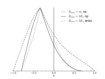
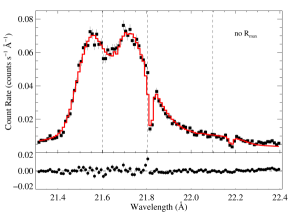
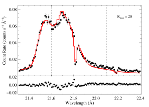
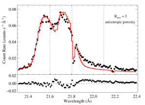
In Figure 7 we show a comparison of models illustrating the effect of a finite upper radial cutoff to the X-ray emission in line profile models. For a given value of $\tau_{*}$, a model with a finite radial cutoff can produce a much more asymmetric line profile. Of course, porosity can mitigate this to some extent. However, note that the models with a finite radial cutoff to X-ray emission have no flux at all in the wings of the profile, since there is no X-ray emitting plasma far out in the wind, where the highest velocities are. This important difference applies to porous models just as much as non-porous models.

Figure 7.— Comparison of three model profiles: a model with no porosity and no upper radial cutoff; a model with no porosity and upper radial cutoff of 5 $R_{*}$; and a model with anisotropic porosity, $h_{\infty}=R_{*}$, and an upper radial cutoff of 5 $R_{*}$. All of the models assume $\tau_{*}=3$. Note that both of the models with a cutoff have corresponding cutoffs to X-ray emission in the wings of the profile.

5.2. Comparison with observed line profiles

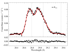
To attempt to reconcile our results with those of Oskinova et al. (2006), we have performed fits to the O VIII line in the RGS spectrum of $\zeta$ Pup assuming the same upper and lower radial bounds to X-ray emission that they used: $R_{0}=1.5R_{*}$ and $R_{\mathrm{max}}=5R_{*}$. We have also fit the same model to the Chandra spectra and get comparable results to the RGS fits, but with lower statistical significance, and we therefore focus on the RGS results in this section.

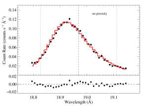
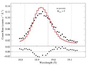
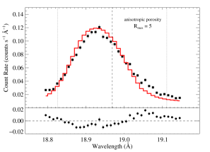
We fit a non-porous model as well as models with both isotropic and anisotropic porosity. The results of our fits are given in Table 8 and the best fit models are shown in Figure 8. Because the fits are formally unacceptable, we do not report model parameter confidence intervals. Note that the model with isotropic clumps preferred no porosity effect in the fit, so we do not list it separately.

The results of our fits assuming finite $R_{\mathrm{max}}$are qualitatively similar to Oskinova et al. We find that under these assumptions, no value of $\tau_{*}$ can provide a good fit to the data in the absence of porosity, while on the other hand we find a much improved fit from an anisotropic porosity model. Nevertheless, the anisotropic porosity model with finite upper radial cutoff does not provide nearly as good a fit as the nonporous model of Table 3 with no upper radial cutoff, which is also shown in the first panel of Figure 8 for comparison. The poor fit of both models with $R_{\mathrm{max}}=5R_{*}$ to the data is due in large part to the lack of flux in the wings of the profile, especially the red wing. This lack of flux in the wings is a necessary consequence of a finite radial upper cutoff.

Table 8Effect of radial bounds of $R_{0}=1.5R_{*}$ and $R_{\mathrm{max}}=5R_{*}$ on fit to O VIII Ly$\alpha$ in XMM-Newton RGS spectrum

$h_{\infty}$	$\tau_{*}$	Type	Normalization	$\chi^{2}$	$N_{\rm bins}$
($R_{*}$)			($10^{-4}$ photons cm-2 s-1)
0	2.34	np, iso	4.404	1421.0	72
1.03	18.46	aniso	4.506	769.6	72

Figure 8.— Three model fits to the O VIII Ly$\alpha$ line in the XMM-Newton RGS spectrum of $\zeta$ Pup. RGS2 data are shown, but the fits are performed simultaneously to data from both RGS. The first panel shows the nonporous fit reported in Section 4. The second panel shows a non-porous model with $R_{0}=1.5R_{*}$ and $R_{\mathrm{max}}=5R_{*}$. The third panel shows a model with anisotropic clumps, and with the same radial cutoffs. The last two panels correspond approximately to the models shown in Figure 8 of Oskinova et al. (2006). (A color version of this figure is available in the online journal.)

5.3. Constraints on the radial upper bound from forbidden line strength

An obvious way to obtain a strong constraint on the presence of hot plasma at large radii is by modeling the weak forbidden lines of the He-like triplets, which are sensitive to the radial distribution of X-ray emitting plasma (Kahn et al., 2001). This sensitivity comes about because the upper level of the forbidden line is metastable, and can be depopulated by photoexcitation from the star’s intense UV radiation field, the strength of which is radially dependent due to geometrical dilution.

The forbidden-to-intercombination line ratio is predicted for different He-like ions as a function of radius in Figure 3 of Leutenegger et al. (2006). It is evident from this plot that the forbidden lines of N VI and O VII are strongly suppressed for $r<20R_{*}$, which already suggests that an upper radial cutoff of $R_{\mathrm{max}}=5R_{*}$ is likely not compatible with the detection of weak forbidden lines. However, as shown in Leutenegger et al. (2006), it is straightforward to include the radial dependence of the $f/i$ ratio in the integrand of the line profile calculation in Equation 1 and test the effects of an upper radial cutoff against the measured He-like complex data.

We fit this model to the O VII and N VI triplets in the RGS spectrum of $\zeta$ Pup. Resonance scattering was included in our models, as described in Leutenegger et al. (2007). The weak C VI Ly$\beta$ line (which falls on the red wing of the resonance line of N VI) was included in our fit to the N VI complex, as in Leutenegger et al. (2007). Both complexes were fit under the competing assumptions that $R_{\mathrm{max}}=\infty$ or $20R_{*}$. In order to make a more direct comparison with the radial distribution of X-ray emitting plasma assumed in Oskinova et al., we also tried to fit the data with models using their values of $R_{0}=1.5R_{*}$ and $R_{\mathrm{max}}=5R_{*}$, and including the effects of porosity by allowing $h_{\infty}$ to be a free parameter. The results of our fits are given in Table 9, and the models are shown in Figures 9 and 10.

The models with a finite radial cutoff clearly do not produce enough emission from the forbidden line to fit the data. On the other hand, the models with no radial cutoff fits the $f/i$ line ratios (and the line complexes) quite well. We thus conclude that a $R_{\mathrm{max}}=5R_{*}$ cutoff is strongly disfavored by the observed forbidden line strengths as well as the wings of individual lines.

Table 9He-like triplet models with finite radial upper cutoff: fit results to the XMM-Newton RGS spectra

ion	$\tau_{*}$	$R_{0}$	$R_{\mathrm{max}}$	$h_{\infty}$	$\tau_{0,*}$	$G$	Normalization	$\chi^{2}$	$N_{\rm bins}$
		($R_{*}$)	($R_{*}$)	($R_{*}$)			($10^{-4}$ photons cm-2 s-1)
N VI	4.79	2.28	$\infty$	0	$\infty$	1.162	17.52	181.5	142
	5.70	4.0	20	0	$\infty$	1.176	16.96	381.5	142
	26.28	1.5	5	0.72	$\infty$	1.085	16.05	1435.9	142
O VII	3.96	1.59	$\infty$	0	2.68	1.005	7.582	146.8	109
	7.75	4.0	20	0	8.32	1.174	7.408	311.1	109
	25.57	1.5	5	0.77	0.85	1.095	7.171	740.8	109

Figure 9.— XMM-Newton RGS spectrum of the O VII complex of $\zeta$ Pup, together with best fit models assuming $R_{\mathrm{max}}=\infty$ (first panel), $R_{\mathrm{max}}=20R_{*}$ (second panel), and $R_{\mathrm{max}}=5R_{*}$ (third panel). The three vertical dashed lines indicate the positions of the rest wavelengths of the resonance, intercombination, and forbidden lines, from left to right. The model shown in third panel includes the effects of anisotropic porosity, and is comparable to the model favored in Oskinova et al. (2006). Both models with finite radial upper cutoffs underpredict emission from the forbidden line, which is primarily formed at large radii. (A color version of this figure is available in the online journal.)

Figure 10.— XMM-Newton RGS spectrum of the N VI complex of $\zeta$ Pup, together with best fit models assuming $R_{\mathrm{max}}=\infty$ (first panel), $R_{\mathrm{max}}=20R_{*}$ (second panel) , and $R_{\mathrm{max}}=5R_{*}$ (third panel). The three vertical dashed lines indicate the positions of the rest wavelengths of the resonance, intercombination, and forbidden lines, from left to right. The model shown in third panel includes the effects of anisotropic porosity, and is comparable to the model favored in Oskinova et al. (2006). Both models with finite radial upper cutoffs underpredict emission from the forbidden line, which is primarily formed at large radii. The weak feature at 28.4656 Å is C VI Ly$\beta$. (A color version of this figure is available in the online journal.)

6. Discussion

One of the most important results of our emission line profile modeling is that anisotropic porosity models are disfavored. This can be understood in terms of the markedly different profile shapes predicted by anisotropic porosity models, with a strong bump at line center due to the “Venetian blind effect”, as exemplified in Figure 6. There is no such bump evident in any of the profiles we have modeled, and this is reflected in our formal statistical constraints.

On the other hand, isotropic porosity models can provide good fits to the lines we studied, provided the porosity lengths are no larger than $R_{*}$. Porosity length and mass-loss rate are degenerate to a certain extent, since they both influence the degree of profile asymmetry. We have quantified this degeneracy for one line in Figure 5. Large porosity lengths ($h_{\infty}>R_{*}$) and their associated large adjustments to derived mass-loss rates are disfavored by the data. Ruling out large porosity lengths is possible because porosity length and mass-loss rate are not fully degenerate parameters, leading to measurable differences in profile shape, as shown in Figure 6. Smaller non-zero porosity lengths are allowed, but lead to only modest adjustments to derived mass-loss rates.

We have compared our results to those of Oskinova et al. (2006), who also compare both porous and non-porous models to X-ray spectra of $\zeta$ Pup, but reach the opposite conclusion that models assuming anisotropic porosity are allowed, and non-porous models disfavored. We showed that this difference in conclusions is a direct result of a difference in assumptions regarding the spatial distribution of X-ray emitting plasma. Specifically, we assumed in our modeling that X-ray emission extends to effectively infinite radius, while Oskinova et al. assumed that X-ray emission turns off above 5 $R_{*}$.

In Figure 7 we compared the effect of different assumptions regarding $R_{\mathrm{max}}$, and found that models with a finite radial cutoff have much less flux in the wings of the line profile than models with no cutoff, which is a straightforward consequence of the fact that all emission at large redshift and blueshift originates at large radii. We fit models with different assumed values for $R_{\mathrm{max}}$to the O VIII Ly$\alpha$ line, and found that models with a finite radial cutoff do not fit the wings of the observed line profile of $\zeta$ Pup.

We further probed the radial distribution of X-ray emission in the wind of $\zeta$ Pup by fitting the He-like triplet lines of O VII and N VI with models accounting for the radial dependence of the forbidden-to-intercombination line ratio (Leutenegger et al., 2006). As is evident from Figures 9 and 10, models with a finite radial cutoff do not reproduce the observed forbidden line flux, which indicates that there is significant X-ray emission originating from $R>20R_{*}$.

The finding of significant X-ray emission from large radii is one of the major, if unintended, results of this study. One might be surprised by this result based on the simple argument that X-rays should originate where the wind is accelerating and can generate strong shocks. Runacres & Owocki (2002) have performed hydrodynamic simulations specifically aimed at understanding the outer wind structure of O stars, and they find that X-ray emitting shocks can be generated at tens of stellar radii. Furthermore, the cooling time for few MK plasma formed at $r\>\vbox{\hbox{$>$\hskip-7.5pt\lower 4.30554pt\hbox{$\sim$}}}\>10R_{*}$ in the wind of $\zeta$ Pup is comparable to the flow time, so even if new shocks are not generated at very large radii, X-ray emission can still persist (Feldmeier et al., 1997a).

Under similar modeling assumptions as Oskinova et al. (2006), in particular that X-ray emission is cut off above 5 $R_{*}$, we too find that porous models with anisotropic clumps are favored over non-porous models. But we also show that such a small cutoff radius for X-ray emission is not consistent with either the observed flux in the wings of X-ray emission lines, or the strength of forbidden line in He-like triplets. These constraints are well matched by models without an arbitrary X-ray cutoff. With such extended emission, fitting line profiles favors models with either no or a modest isotropic porosity, with anisotropic porosity strongly disfavored.

Cohen et al. (2010) have derived a mass-loss rate for $\zeta$ Pup from modeling of X-ray line profiles under the assumption that porosity effects are negligible. Taking the conclusions of the present work at face value, the correction to this mass-loss rate is at most 40 % if moderate porosity effects are present ($h_{\infty}\sim R_{*}$). This conclusion is further supported by the fact that the uncorrected X-ray mass-loss rate of Cohen et al. (2010) agrees with mass-loss rates from non-X-ray observational diagnostics within uncertainties (Najarro et al., 2011; Bouret et al., 2012).

We thus conclude that, at least for $\zeta$ Pup, X-ray line profiles are a good independent diagnostic of mass-loss rates, and that they are not subject to strong systematic errors from clumping on any scale. The other O stars observed by Chandra and XMM-Newton should ideally also be subjected to a similar study, although it would perhaps be surprising to find major differences in porosity effects in the wind of $\zeta$ Pup in comparison with other O stars. In fact, early O supergiants like $\zeta$ Pup with their high mass-loss-rate winds are the stars for which porosity effects are expected to be the strongest. Because the essence of porosity is the optical thickness of individual clumps, O stars with lower mass-loss rates than $\zeta$ Pup require more extreme clump properties just to produce the same porosity effect.

The relative robustness against wind inhomogeneity effects of X-ray line profile measurements of mass-loss rates suggests their use as a primary mass-loss rate diagnostic, on an equal footing with traditional diagnostics such as H$\alpha$, thermal radio emission, and UV absorption line profiles. However, X-ray line profile measurements are currently only possible for the brightest stars in the Galaxy. Until the advent of much larger X-ray spectroscopic observatories, with square meter effective areas and which could undertake a large-scale survey of O star X-ray spectra, we suggest a program of benchmarking as many stars as possible with all available mass-loss rate diagnostics. Only by continuing the tradition of a multiwavelength, multidiagnostic approach can we hope to disentangle the observational signatures of mass-loss and wind structure.

Appendix A Expanded fit results

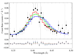
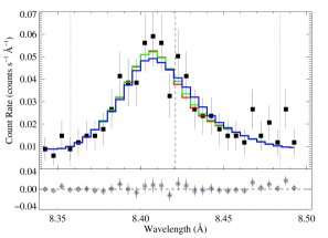
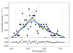
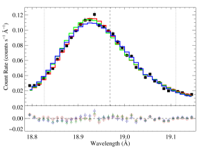
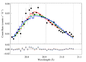
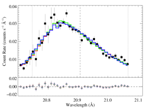
In this section, in Figures 11-20 we show plots of all the fits reported in Tables 4-7. For each line that we fit, we show plots of anisotropic porosity models in one figure, and isotropic porosity models in another figure. We repeat the non-porous model in both the anisotropic and isotropic porosity fit figures. To keep the figures legible, we only show models with $h_{\infty}$ = 0, 1, and 5 $R_{*}$.

Figure 11.— The Chandra MEG measurements of the Mg XII line at 8.421 Å, with the best-fit anisotropic porosity models superimposed. The red, green, and blue models assume $h_{\infty}$ = 0, 1, and 5 $R_{*}$, respectively. (A color version of this figure is available in the online journal.)

Figure 12.— The Chandra MEG measurements of the Mg XII line at 8.421 Å, with the best-fit isotropic porosity models superimposed. The red, green, and blue models assume $h_{\infty}$ = 0, 1, and 5 $R_{*}$, respectively. (A color version of this figure is available in the online journal.)

Figure 13.— The Chandra MEG (upper panel) and XMM-Newton RGS (lower panel) measurements of the Ne X line at 12.134 Å, with the best-fit anisotropic porosity models superimposed. The red, green, and blue models assume $h_{\infty}$ = 0, 1, and 5 $R_{*}$, respectively. (A color version of this figure is available in the online journal.)

Figure 14.— The Chandra MEG (upper panel) and XMM-Newton RGS (lower panel) measurements of the Ne X line at 12.134 Å, with the best-fit isotropic porosity models superimposed. The red, green, and blue models assume $h_{\infty}$ = 0, 1, and 5 $R_{*}$, respectively. (A color version of this figure is available in the online journal.)

Figure 15.— The Chandra MEG measurements of the Fe XVII line at 16.780 Å, with the best-fit anisotropic porosity models superimposed. The red, green, and blue models assume $h_{\infty}$ = 0, 1, and 5 $R_{*}$, respectively. (A color version of this figure is available in the online journal.)

Figure 16.— The Chandra MEG measurements of the Fe XVII line at 16.780 Å, with the best-fit isotropic porosity models superimposed. The red, green, and blue models assume $h_{\infty}$ = 0, 1, and 5 $R_{*}$, respectively. (A color version of this figure is available in the online journal.)

Figure 17.— The Chandra MEG (upper panel) and XMM-Newton RGS (lower panel) measurements of the O VIII line at 18.969 Å, with the best-fit anisotropic porosity models superimposed. The red, green, and blue models assume $h_{\infty}$ = 0, 1, and 5 $R_{*}$, respectively. (A color version of this figure is available in the online journal.)

Figure 18.— The Chandra MEG (upper panel) and XMM-Newton RGS (lower panel) measurements of the O VIII line at 18.969 Å, with the best-fit isotropic porosity models superimposed. The red, green, and blue models assume $h_{\infty}$ = 0, 1, and 5 $R_{*}$, respectively. (A color version of this figure is available in the online journal.)

Figure 19.— The XMM-Newton RGS measurements of the N VII line at 20.910 Å, with the best-fit anisotropic porosity models superimposed. The red, green, and blue models assume $h_{\infty}$ = 0, 1, and 5 $R_{*}$, respectively. (A color version of this figure is available in the online journal.)

Figure 20.— The XMM-Newton RGS measurements of the N VII line at 20.910 Å, with the best-fit isotropic porosity models superimposed. The red, green, and blue models assume $h_{\infty}$ = 0, 1, and 5 $R_{*}$, respectively. (A color version of this figure is available in the online journal.)

References

- Arnaud (1996) Arnaud, K. A. 1996, in ASP Conf. Ser., Vol. 101, Astronomical Data Analysis Software and Systems V, ed. G. H. Jacoby & J. Barnes, (San Francisco, CA: ASP), 17
- Bouret et al. (2012) Bouret, J.-C., Hillier, D. J., Lanz, T., & Fullerton, A. W. 2012, A&A, 544, A67
- Brucato (1971) Brucato, R. J. 1971, MNRAS, 153, 435
- Cash (1979) Cash, W. 1979, ApJ, 228, 939
- Churazov et al. (1996) Churazov, E., Gilfanov, M., Forman, W., & Jones, C. 1996, ApJ, 471, 673
- Cohen et al. (2010) Cohen, D. H., Leutenegger, M. A., Wollman, E. E., Zsargó, J., Hillier, D. J., Townsend, R. H. D., & Owocki, S. P. 2010, MNRAS, 405, 2391
- Coia & Pollock (2008) Coia, D., & Pollock, A. M. T. 2008, XMM-Newton Calibration Document CAL-TN-0080
- den Herder et al. (2001) den Herder, J. W., et al. 2001, A&A, 365, L7
- Feldmeier et al. (1997a) Feldmeier, A., Kudritzki, R.-P., Palsa, R., Pauldrach, A. W. A., & Puls, J. 1997a, A&A, 320, 899
- Feldmeier et al. (2003) Feldmeier, A., Oskinova, L., & Hamann, W.-R. 2003, A&A, 403, 217
- Feldmeier et al. (1997b) Feldmeier, A., Puls, J., & Pauldrach, A. W. A. 1997b, A&A, 322, 878
- Fullerton et al. (2006) Fullerton, A. W., Massa, D. L., & Prinja, R. K. 2006, ApJ, 637, 1025
- Haser (1995) Haser, S. M. 1995, PhD thesis, Universitäts-Sternwarte der Ludwig-Maximillian Universität, München, (1995)
- Kahn et al. (2001) Kahn, S. M., Leutenegger, M. A., Cottam, J., Rauw, G., Vreux, J.-M., den Boggende, A. J. F., Mewe, R., & Güdel, M. 2001, A&A, 365, L312
- Leutenegger et al. (2007) Leutenegger, M. A., Owocki, S. P., Kahn, S. M., & Paerels, F. B. S. 2007, ApJ, 659, 642
- Leutenegger et al. (2006) Leutenegger, M. A., Paerels, F. B. S., Kahn, S. M., & Cohen, D. H. 2006, ApJ, 650, 1096
- Lucy & Solomon (1970) Lucy, L. B., & Solomon, P. M. 1970, ApJ, 159, 879
- Lucy & White (1980) Lucy, L. B., & White, R. L. 1980, ApJ, 241, 300
- Massa et al. (2003) Massa, D., Fullerton, A. W., Sonneborn, G., & Hutchings, J. B. 2003, ApJ, 586, 996
- Morton (1967) Morton, D. C. 1967, ApJ, 147, 1017
- Najarro et al. (2011) Najarro, F., Hanson, M. M., & Puls, J. 2011, A&A, 535, A32
- Nazé et al. (2012) Nazé, Y., Flores, C. A., & Rauw, G. 2012, A&A, 538, A22
- Oskinova et al. (2004) Oskinova, L. M., Feldmeier, A., & Hamann, W.-R. 2004, A&A, 422, 675
- Oskinova et al. (2006) —. 2006, MNRAS, 372, 313
- Oskinova et al. (2007) Oskinova, L. M., Hamann, W.-R., & Feldmeier, A. 2007, A&A, 476, 1331
- Owocki (2008) Owocki, S. P. 2008, in Clumping in Hot-Star Winds, ed. W.-R. Hamann, A. Feldmeier, & L. M. Oskinova (Universitätsverlag Potsdam), 121
- Owocki et al. (1988) Owocki, S. P., Castor, J. I., & Rybicki, G. B. 1988, ApJ, 335, 914
- Owocki & Cohen (2001) Owocki, S. P., & Cohen, D. H. 2001, ApJ, 559, 1108
- Owocki & Cohen (2006) —. 2006, ApJ, 648, 565
- Press et al. (2007) Press, W. H., Teukolsky, S. A., Vetterling, W. T., & Flannery, B. P. 2007, Numerical Recipes. The Art of Scientific Computing (3rd ed.; Cambridge: Cambridge Univ. Press)
- Puls et al. (2006) Puls, J., Markova, N., Scuderi, S., Stanghellini, C., Taranova, O. G., Burnley, A. W., & Howarth, I. D. 2006, A&A, 454, 625
- Runacres & Owocki (2002) Runacres, M. C., & Owocki, S. P. 2002, A&A, 381, 1015
- Sundqvist et al. (2012) Sundqvist, J. O., Owocki, S. P., Cohen, D. H., Leutenegger, M. A., & Townsend, R. H. D. 2012, MNRAS, 420, 1553
- Sundqvist et al. (2010) Sundqvist, J. O., Puls, J., & Feldmeier, A. 2010, A&A, 510, A11+
- Sundqvist et al. (2011) Sundqvist, J. O., Puls, J., Feldmeier, A., & Owocki, S. P. 2011, A&A, 528, A64+