aainstitutetext: Department of Physics, University of Waterloo,
Waterloo, Ontario N2L 3G1,Canada
bbinstitutetext: Perimeter Institute for Theoretical Physics,
31 Caroline Street North, Waterloo, Ontario N2L 2Y5, Canada

Deformations of Lifshitz holography with the Gauss-Bonnet term in (n+1𝑛1n+1) dimensions

Miok Park a,b    and Robert B. Mann m7park@sciborg.uwaterloo.ca rbmann@sciborg.uwaterloo.ca
Abstract

We investigate deformations of Gauss-Bonnet-Lifshitz holography in (n+1)𝑛1(n+1) dimensional spacetime. Marginally relevant operators are dynamically generated by a momentum scale Λ0similar-toΛ0\Lambda\sim 0 and correspond to slightly deformed Gauss-Bonnet-Lifshitz spacetimes via a holographic picture. To admit (non-trivial) sub-leading orders of the asymptotic solution for the marginal mode, we find that the value of the dynamical critical exponent z𝑧z is restricted by z=n12(n2)α~𝑧𝑛12𝑛2~𝛼z=n-1-2(n-2)\tilde{\alpha}, where α~~𝛼\tilde{\alpha} is the (rescaled) Gauss-Bonnet coupling constant. The generic black hole solution, which is characterized by the horizon flux of the vector field and α~~𝛼\tilde{\alpha}, is obtained in the bulk, and we explore its thermodynamic properties for various values of n𝑛n and α~~𝛼\tilde{\alpha}.

Keywords:
Lifshitz, Holographic Correspondence, Gravity/Gauge duality, Holographic Renormalization, Boundary Terms, Surface Terms, Variational Principle, Higher Curvature, Gauss-Bonnet, Quantum Critical Theory, Quantum Criticality
arxiv: arXiv:1305.5578

1.  Introduction

Inspired by the AdS/CFT correspondence Maldacena:1997re , new applications of the holographic correspondence principle are being explored in many strongly coupled systems such as AdS/QCD duality Forkel:2007cm ; Gursoy:2007cb ; Hoyos:2006gb , gravity/condensed matter theory duality (AdS/CMT) Bertoldi:2009dt ; Braviner:2011kz ; Hartnoll:2009sz ; Horowitz:2010gk ; Kachru:2008yh ; Mann:2011hg ; Ross:2011gu or gravity/fluid duality Bredberg:2010ky ; Janik:2005zt ; Rangamani:2009xk .

Since metallic systems that are strongly coupled can be engineered in laboratories, the AdS/CMT correspondence provides the possibility of direct experimental tests. One interesting avenue of study has emerged from quantum critical phenomena associated with continuous phase transitions, which shows unusual behaviour such as a vanishing characteristic energy scale and a diverging correlation length scale at the quantum critical point g=gc𝑔subscript𝑔𝑐g=g_{c}. In the vicinity of the critical point, it is also observed that temporal correlations of the order parameter decay slower and slower as one approaches the critical point. Thus time scales differently from space in this limit, yielding a scaling symmetry

tλzt,xλxformulae-sequence𝑡superscript𝜆𝑧𝑡𝑥𝜆𝑥t\rightarrow\lambda^{z}t,\qquad\vec{x}\rightarrow\lambda\;\vec{x} (1.1)

where z𝑧z is the dynamical critical exponent; z=1𝑧1z=1 corresponds to conformal invariance, whereas z1𝑧1z\neq 1 represents an anisotropic scaling invariance.

From the perspective of holographic correspondence, this anisotropic symmetry can be geometrically configured via

ds2=l2(dt2r2z+dr2r2+dx12+dx22r2)𝑑superscript𝑠2superscript𝑙2𝑑superscript𝑡2superscript𝑟2𝑧𝑑superscript𝑟2superscript𝑟2𝑑superscriptsubscript𝑥12𝑑superscriptsubscript𝑥22superscript𝑟2ds^{2}=l^{2}\bigg{(}-\frac{dt^{2}}{r^{2z}}+\frac{dr^{2}}{r^{2}}+\frac{dx_{1}^{2}+dx_{2}^{2}}{r^{2}}\bigg{)} (1.2)

which is called Lifshitz spacetime for z1𝑧1z\neq 1 and obviously satisfies

tλzt,rλr,xλx.formulae-sequence𝑡superscript𝜆𝑧𝑡formulae-sequence𝑟𝜆𝑟𝑥𝜆𝑥t\rightarrow\lambda^{z}t,\qquad r\rightarrow\lambda\;r,\qquad\vec{x}\rightarrow\lambda\;\vec{x}. (1.3)

When z1𝑧1z\neq 1, the non-trivial metric (1.2) can be generated by having an anisotropic energy-momentum tensor that is supported by a massive vector field. Alternatively adding higher curvature terms such as R2superscript𝑅2R^{2}, Gauss-Bonnet, or Lovelock terms into the action can also engender an anisotropy of spacetime. Whereas when z=1𝑧1z=1, the metric (1.2) with (1.3) restores the (asymptotic) AdS spacetime. In this paper, we consider the effects of both the massive vector field and the Gauss-Bonnet term in (n+1𝑛1n+1) dimensional spacetime, extending previous investigations along these lines Cheng:2009df ; Park:2012mn .

Gauss-Bonnet gravity generalizes Einstein gravity to include quadratic curvature terms. The equations of motion consist of the Einstein equations modified by additional quadratic curvature terms (with coupling constant α𝛼\alpha) in such a way that the higher derivative terms cancel out. The additional terms in the equations of motion identically vanish in four dimensional spacetime, and so effects from such terms are manifest only in 5 dimensions or more. There are various motivations for considering such higher dimensional gravitational theories.

In gravity theory, considering higher curvature terms expands the array of black hole solutions in Einstein gravity to Gauss-Bonnet-Einstein black hole solutions. Examples include the Boulware-Deser solution for spherically symmetric spacetime Boulware:1985wk ,Wheeler:1985nh and the Gauss-Bonnet black hole solution in AdS spacetime Cai:2001dz ,Cho:2002hq ,Cvetic:2001bk ,Neupane:2002bf , and the properties of these black hole solutions have been studied Jacobson:1993xs ,Torii:2005xu . In supersting/M-theory the Gauss-Bonnet term naturally arises in effective low energy limit and leads to ghost-free nontrivial gravitational self interactions Zwiebach:1985uq . Also in cosmology, it provides one approach to understand the current acceleration of the universe in the context of the dark energy problem Leith:2007bu ,Nojiri:2005jg . In brane-world scenarios it yields additional interesting features Charmousis:2002rc ,Davis:2002gn . From the holographic correspondence point of view, involving condensed matter systems, one expects that the higher curvature correction will induce interesting new effects Gregory:2009fj ,Kanno:2011cs or provide a better explanation for physical phenomena shown in abnormal materials.

The main purpose of this paper is to find what role the Gauss-Bonnet coupling plays in deformed Gauss-Bonnet-Lifshitz (GB-Lifshitz) holography. In 5 dimensions this is the simplest extension that can yield interesting effects in a four-dimensional theory; we shall here examine any dimensionality. To do so, we assume GB-Lifshitz spacetime in the ultraviolet (UV) energy regime and Gauss-Bonnet-AdS (GB-AdS) spacetime in the infrared (IR) energy regime, and consider the special condition z=(n1)2(n2)α~𝑧𝑛12𝑛2~𝛼z=(n-1)-2(n-2)\tilde{\alpha}, where z𝑧z is the dynamic critical exponent and α~~𝛼\tilde{\alpha} is the rescaled Gauss-Bonnet coupling constant (defined below). This condition allows us to describe the marginally relevant operator, when the operator is expanded to sub-leading orders. To generate the sub-leading orders of the gravitational solutions at the boundary, we introduce a momentum scale ΛΛ\Lambda, which is very small (Λ0similar-toΛ0\Lambda\sim 0) and expand the solutions as a power series in this quantity. Then these sub-leading terms slightly deform the GB-Lifshitz spacetime, which lies in high energy scale Λz/T0superscriptΛ𝑧𝑇0\Lambda^{z}/T\rightarrow 0, at the asymptotic region. We also consider the finite temperature theory by finding (planar) black hole solutions, which are expanded near the horizon. From the duality perspective, this configuration leads us to expect that the gravitational solution at the boundary of the deformed spacetime gives information about how marginally relevant operators behave near critical points at finite temperature in quantum critical theory. Thus we observe the behaviours of the physical quantities such as the free energy density or the energy density, which shows the properties of the marginally relevant operators, according to different values of α~~𝛼\tilde{\alpha} for given horizon flux of a massive vector field. At the zero temperature limit Λz/TsuperscriptΛ𝑧𝑇\Lambda^{z}/T\rightarrow\infty (at fixed Λ0similar-toΛ0\Lambda\sim 0) the GB-AdS spacetime can emerge; it then might be possible to find the renormalization group flow between the deformed GB-Lifshitz and GB-AdS spacetime, as per the AdS case Braviner:2011kz ,Kachru:2008yh .

In section 2, the Gauss-Bonnet-Einstein action with negative cosmological constant coupled to a massive vector field is introduced, and its equations of motion are derived. In section 3, we consider asymptotically Lifshitz spacetime in the high energy regime, slightly deformed by a small value ΛΛ\Lambda, and calculate its asymptotic solutions. In section 4, with these asymptotic solutions we perform holographic renormalization by constructing the relevant counterterms so as to achieve a well-defined action principle. By doing so, we obtain a well-defined free energy density \mathcal{F} and energy density \mathcal{E}. Moving near the black hole horizon, in section 5, we derive the expanded black hole solutions in this region, and obtain the thermodynamic variables defined at the horizon. Also we check that our analytic calculations agree with the integrated form of the first thermodynamic law. In section 6, we carry out numerical work with the asymptotic solutions and the expanded black hole solutions. Choosing various values of α~=14,110,0,120,12(n2),310~𝛼14110012012𝑛2310\tilde{\alpha}=\frac{1}{4},\frac{1}{10},0,-\frac{1}{20},-\frac{1}{2(n-2)},-\frac{3}{10}, we then fix the undetermined parameters (ΛΛ\Lambda, f0subscript𝑓0f_{0}, and p0subscript𝑝0p_{0}) appearing in the metric for given α~~𝛼\tilde{\alpha} and h0subscript0h_{0}, which are variables characterizing black hole solution, using numerical integration. Based on these fixed values, we explore the physical quantities, and finally plot the free energy density and the energy density depending log(Λz/T)superscriptΛ𝑧𝑇\log(\Lambda^{z}/T) and find their fitting functions. In section 7, we summarize and discuss our work.

2.  Higher curvature gravity with a massive vector field

We start with (n+1)𝑛1(n+1) dimensional gravitational action modified by higher curvature terms and coupled to a massive vector field

S=dn+1xg(12κn+12[R+2Λ~+αGB]1gv2[14H2+γ2B2])𝑆superscript𝑑𝑛1𝑥𝑔12superscriptsubscript𝜅𝑛12delimited-[]𝑅2~Λ𝛼subscript𝐺𝐵1superscriptsubscript𝑔𝑣2delimited-[]14superscript𝐻2𝛾2superscript𝐵2S=\int d^{n+1}x\sqrt{-g}\bigg{(}\frac{1}{2\kappa_{n+1}^{2}}[R+2\tilde{\Lambda}+\alpha{\mathcal{L}_{GB}}]-\frac{1}{{g_{v}}^{2}}\bigg{[}\frac{1}{4}H^{2}+\frac{\gamma}{2}B^{2}\bigg{]}\bigg{)} (2.1)

where κn+1=8πGn+1subscript𝜅𝑛18𝜋subscript𝐺𝑛1\kappa_{n+1}=\sqrt{8\pi G_{n+1}}, Λ~~Λ\tilde{\Lambda} is cosmological constant, α𝛼\alpha is the Gauss-Bonnet coupling constant and GB=R24RμνRμν+RμναβRμναβsubscript𝐺𝐵superscript𝑅24subscript𝑅𝜇𝜈superscript𝑅𝜇𝜈subscript𝑅𝜇𝜈𝛼𝛽superscript𝑅𝜇𝜈𝛼𝛽{\mathcal{L}_{GB}}=R^{2}-4R_{\mu\nu}R^{\mu\nu}+R_{\mu\nu\alpha\beta}R^{\mu\nu\alpha\beta}. H=dB𝐻𝑑𝐵H=dB, and gvsubscript𝑔𝑣g_{v} and γ𝛾\gamma are the coupling constant and the squared mass of the vector field respectively. This action yields equations of motion for the gravitational field

Gμν+αLμνΛ~gμν=κn+12Tμνsubscript𝐺𝜇𝜈𝛼subscript𝐿𝜇𝜈~Λsubscript𝑔𝜇𝜈superscriptsubscript𝜅𝑛12subscript𝑇𝜇𝜈G_{\mu\nu}+\alpha L_{\mu\nu}-\tilde{\Lambda}g_{\mu\nu}={\kappa_{n+1}^{2}}T_{\mu\nu} (2.2)

where

Gμν=Rμν12gμνR,subscript𝐺𝜇𝜈subscript𝑅𝜇𝜈12subscript𝑔𝜇𝜈𝑅\displaystyle G_{\mu\nu}=R_{\mu\nu}-\frac{1}{2}g_{\mu\nu}R, (2.3)
Lμν=2(RRμν2RμαRνα2RαβRμανβ+RμαβγRναβγ)12gμνGB,subscript𝐿𝜇𝜈2𝑅subscript𝑅𝜇𝜈2subscript𝑅𝜇𝛼subscriptsuperscript𝑅𝛼𝜈2superscript𝑅𝛼𝛽subscript𝑅𝜇𝛼𝜈𝛽superscriptsubscript𝑅𝜇𝛼𝛽𝛾subscript𝑅𝜈𝛼𝛽𝛾12subscript𝑔𝜇𝜈subscript𝐺𝐵\displaystyle L_{\mu\nu}=2\bigg{(}RR_{\mu\nu}-2R_{\mu\alpha}R^{\alpha}_{\;\;\nu}-2R^{\alpha\beta}R_{\mu\alpha\nu\beta}+R_{\mu}^{\;\;\alpha\beta\gamma}R_{\nu\alpha\beta\gamma}\bigg{)}-\frac{1}{2}g_{\mu\nu}{\mathcal{L}_{GB}}, (2.4)
Tμν=1gv2(HμρHνρ14gμνH2)+γgv2(BμBν12gμνB2),subscript𝑇𝜇𝜈1superscriptsubscript𝑔𝑣2subscript𝐻𝜇𝜌superscriptsubscript𝐻𝜈𝜌14subscript𝑔𝜇𝜈superscript𝐻2𝛾superscriptsubscript𝑔𝑣2subscript𝐵𝜇subscript𝐵𝜈12subscript𝑔𝜇𝜈superscript𝐵2\displaystyle T_{\mu\nu}=\frac{1}{{g_{v}}^{2}}\bigg{(}H_{\mu\rho}H_{\nu}^{\;\rho}-\frac{1}{4}g_{\mu\nu}H^{2}\bigg{)}+\frac{\gamma}{{g_{v}}^{2}}\bigg{(}B_{\mu}B_{\nu}-\frac{1}{2}g_{\mu\nu}B^{2}\bigg{)}, (2.5)

and for the massive vector field

μHμνγBν=0.subscript𝜇superscript𝐻𝜇𝜈𝛾superscript𝐵𝜈0\nabla_{\mu}H^{\mu\nu}-\gamma B^{\nu}=0. (2.6)

At the asymptotic region (i.e. r0𝑟0r\rightarrow 0), for z1𝑧1z\neq 1 we require the equations of motion to admit the metric

ds2=l2(dt2r2z+dr2r2+dx2+dy2+r2)𝑑superscript𝑠2superscript𝑙2𝑑superscript𝑡2superscript𝑟2𝑧𝑑superscript𝑟2superscript𝑟2𝑑superscript𝑥2𝑑superscript𝑦2superscript𝑟2ds^{2}=l^{2}\bigg{(}-\frac{dt^{2}}{r^{2z}}+\frac{dr^{2}}{r^{2}}+\frac{dx^{2}+dy^{2}+\cdots}{r^{2}}\bigg{)} (2.7)

which is supported by the vector potential described by

B=gvlκn+1qrzdt.𝐵subscript𝑔𝑣𝑙subscript𝜅𝑛1𝑞superscript𝑟𝑧𝑑𝑡B=\frac{g_{v}l}{\kappa_{n+1}}\frac{q}{r^{z}}dt. (2.8)

These ansatz and boundary conditions fine-tune the cosmological constant to be

Λ~=χ12l2α~χ2l2~Λsubscript𝜒12superscript𝑙2~𝛼subscript𝜒2superscript𝑙2\tilde{\Lambda}=\frac{\chi_{1}}{2l^{2}}-\tilde{\alpha}\frac{\chi_{2}}{l^{2}} (2.9)

where we replaced the coupling constant of the Gauss-Bonnet α𝛼\alpha with α~~𝛼\tilde{\alpha}, which is

α~=α(n2)(n3)l2,~𝛼𝛼𝑛2𝑛3superscript𝑙2\tilde{\alpha}=\frac{\alpha(n-2)(n-3)}{l^{2}}, (2.10)

and the squared mass and the squared charge to be

γ=(n1)zl2,q2=z1z(12α~)formulae-sequence𝛾𝑛1𝑧superscript𝑙2superscript𝑞2𝑧1𝑧12~𝛼\gamma=\frac{(n-1)z}{l^{2}},\;\;\;\;\;\;\;q^{2}=\frac{z-1}{z}(1-2\tilde{\alpha}) (2.11)

where the χ1subscript𝜒1\chi_{1} and χ2subscript𝜒2\chi_{2} are defined by

χ1=z2+(n2)z+(n1)2,χ2=z2+(n2)z+(n1)(n2)2.formulae-sequencesubscript𝜒1superscript𝑧2𝑛2𝑧superscript𝑛12subscript𝜒2superscript𝑧2𝑛2𝑧𝑛1𝑛22\chi_{1}=z^{2}+(n-2)z+(n-1)^{2},\;\;\;\;\;\;\;\chi_{2}=z^{2}+(n-2)z+\frac{(n-1)(n-2)}{2}. (2.12)

For given (n,z,α)𝑛𝑧𝛼(n,z,\alpha) we require that AdSn+1 spacetime is also a solution to the equations with cosmological constant (2.9). In this case the metric is

dsAdS2=al2(dt2r2+dr2r2+dx2+dy2+r2)𝑑subscriptsuperscript𝑠2𝐴𝑑𝑆𝑎superscript𝑙2𝑑superscript𝑡2superscript𝑟2𝑑superscript𝑟2superscript𝑟2𝑑superscript𝑥2𝑑superscript𝑦2superscript𝑟2ds^{2}_{AdS}=a\;l^{2}\bigg{(}-\frac{dt^{2}}{r^{2}}+\frac{dr^{2}}{r^{2}}+\frac{dx^{2}+dy^{2}+\cdots}{r^{2}}\bigg{)} (2.13)

where the a𝑎a is the scaling constant defined by

a=n(n1)+n(n1)(12α~)(n(n1)4χ2α~)2(χ12χ2α~)𝑎𝑛𝑛1𝑛𝑛112~𝛼𝑛𝑛14subscript𝜒2~𝛼2subscript𝜒12subscript𝜒2~𝛼a=\frac{n(n-1)+\sqrt{n(n-1)(1-2\tilde{\alpha})(n(n-1)-4\chi_{2}\tilde{\alpha})}}{2(\chi_{1}-2\chi_{2}\tilde{\alpha})} (2.14)

appears because the cosmological constant (2.9) has been already fixed due to the Lifshitz boundary condition.

In order to configure the spacetime to induce renormalization flow from UV Lifshitz spacetime to IR AdS spacetime at finite temperature (thereby recovering isotropic scaling symmetry at low energy), we employ the ansatz

ds2𝑑superscript𝑠2\displaystyle ds^{2} =l2(f(r)dt2+dr2r2+p(r)(dx2+dy2+)),absentsuperscript𝑙2𝑓𝑟𝑑superscript𝑡2𝑑superscript𝑟2superscript𝑟2𝑝𝑟𝑑superscript𝑥2𝑑superscript𝑦2\displaystyle=l^{2}\bigg{(}-f(r)dt^{2}+\frac{dr^{2}}{r^{2}}+p(r)(dx^{2}+dy^{2}+\cdots)\bigg{)}, (2.15)
B𝐵\displaystyle B =gvlκn+1h(r)dt,absentsubscript𝑔𝑣𝑙subscript𝜅𝑛1𝑟𝑑𝑡\displaystyle=\frac{g_{v}l}{\kappa_{n+1}}h(r)dt, (2.16)

and these yield the solution for the GB-Lifshitz spacetime

GB-Lifshitz :f=1r2z,p=1r2,h=(z1)(12α~)z1rzformulae-sequenceGB-Lifshitz :𝑓1superscript𝑟2𝑧formulae-sequence𝑝1superscript𝑟2𝑧112~𝛼𝑧1superscript𝑟𝑧\textrm{GB-Lifshitz :}\;\;\;\;f=\frac{1}{r^{2z}},\;\;p=\frac{1}{r^{2}},\;\;h=\frac{\sqrt{(z-1)(1-2\tilde{\alpha})}}{\sqrt{z}}\frac{1}{r^{z}} (2.17)

and for GB-AdSn+1 spacetime

Gb-AdS :f=p=ar2/a,h=0.formulae-sequenceGb-AdS :𝑓𝑝𝑎superscript𝑟2𝑎0\textrm{Gb-AdS :}\;\;\;\;f=p=ar^{-2/\sqrt{a}},\;\;h=0. (2.18)

Plugging the ansatz (2.15) and (2.16) into (2.2) and (2.6) yields

2zh(r)2f(r)rp(r)p(r)+r2f(r)p(r)2f(r)p(r)+r2p(r)22p(r)2r2p′′(r)p(r)+α~2(r3p(r)3p(r)r4f(r)p(r)32f(r)p(r)3\displaystyle-\frac{2zh(r)^{2}}{f(r)}-\frac{rp^{\prime}(r)}{p(r)}+\frac{r^{2}f^{\prime}(r)p^{\prime}(r)}{2f(r)p(r)}+\frac{r^{2}p^{\prime}(r)^{2}}{2p(r)^{2}}-\frac{r^{2}p^{\prime\prime}(r)}{p(r)}+\frac{\tilde{\alpha}}{2}\bigg{(}\frac{r^{3}p^{\prime}(r)^{3}}{p(r)}-\frac{r^{4}f^{\prime}(r)p^{\prime}(r)^{3}}{2f(r)p(r)^{3}}
r4p(r)42p(r)4+r4p(r)2p′′(r)p(r)3)=0,\displaystyle-\frac{r^{4}p^{\prime}(r)^{4}}{2p(r)^{4}}+\frac{r^{4}p^{\prime}(r)^{2}p^{\prime\prime}(r)}{p(r)^{3}}\bigg{)}=0, (2.19)
2χ1+2(2n3)zh(r)2f(r)rf(r)f(r)+r2f(r)22f(r)2(3n5)r2f(r)p(r)2f(r)p(r)(n2)2r2p(r)22p(r)2r2f′′(r)f(r)2subscript𝜒122𝑛3𝑧superscript𝑟2𝑓𝑟𝑟superscript𝑓𝑟𝑓𝑟superscript𝑟2superscript𝑓superscript𝑟22𝑓superscript𝑟23𝑛5superscript𝑟2superscript𝑓𝑟superscript𝑝𝑟2𝑓𝑟𝑝𝑟superscript𝑛22superscript𝑟2superscript𝑝superscript𝑟22𝑝superscript𝑟2superscript𝑟2superscript𝑓′′𝑟𝑓𝑟\displaystyle 2\chi_{1}+\frac{2(2n-3)zh(r)^{2}}{f(r)}-\frac{rf^{\prime}(r)}{f(r)}+\frac{r^{2}f^{\prime}(r)^{2}}{2f(r)^{2}}-\frac{(3n-5)r^{2}f^{\prime}(r)p^{\prime}(r)}{2f(r)p(r)}-\frac{(n-2)^{2}r^{2}p^{\prime}(r)^{2}}{2p(r)^{2}}-\frac{r^{2}f^{\prime\prime}(r)}{f(r)}
+α~(4χ2+3r3f(r)p(r)22f(r)p(r)2r4f(r)2p(r)24f(r)2p(r)2r3p(r)3p(r)3+3(n3)r4f(r)p(r)34f(r)p(r)3\displaystyle+\tilde{\alpha}\bigg{(}-4\chi_{2}+\frac{3r^{3}f^{\prime}(r)p^{\prime}(r)^{2}}{2f(r)p(r)^{2}}-\frac{r^{4}f^{\prime}(r)^{2}p^{\prime}(r)^{2}}{4f(r)^{2}p(r)^{2}}-\frac{r^{3}p^{\prime}(r)^{3}}{p(r)^{3}}+\frac{3(n-3)r^{4}f^{\prime}(r)p^{\prime}(r)^{3}}{4f(r)p(r)^{3}}
+(n27n+16)r4p(r)48p(r)4+r4p(r)2f′′(r)2f(r)p(r)2+r4f(r)p(r)p′′(r)f(r)p(r)2r4p(r)2p′′(r)p(r)3)=0,\displaystyle+\frac{(n^{2}-7n+16)r^{4}p^{\prime}(r)^{4}}{8p(r)^{4}}+\frac{r^{4}p^{\prime}(r)^{2}f^{\prime\prime}(r)}{2f(r)p(r)^{2}}+\frac{r^{4}f^{\prime}(r)p^{\prime}(r)p^{\prime\prime}(r)}{f(r)p(r)^{2}}-\frac{r^{4}p^{\prime}(r)^{2}p^{\prime\prime}(r)}{p(r)^{3}}\bigg{)}=0, (2.20)
χ1+(n1)zh(r)2f(r)r2h(r)2f(r)(n1)r2f(r)p(r)2f(r)p(r)(n1)(n2)r2p(r)24p(r)2subscript𝜒1𝑛1𝑧superscript𝑟2𝑓𝑟superscript𝑟2superscriptsuperscript𝑟2𝑓𝑟𝑛1superscript𝑟2superscript𝑓𝑟superscript𝑝𝑟2𝑓𝑟𝑝𝑟𝑛1𝑛2superscript𝑟2superscript𝑝superscript𝑟24𝑝superscript𝑟2\displaystyle\chi_{1}+\frac{(n-1)zh(r)^{2}}{f(r)}-\frac{r^{2}h^{\prime}(r)^{2}}{f(r)}-\frac{(n-1)r^{2}f^{\prime}(r)p^{\prime}(r)}{2f(r)p(r)}-\frac{(n-1)(n-2)r^{2}p^{\prime}(r)^{2}}{4p(r)^{2}}
+α~(2χ2+(n1)r4f(r)p(r)34f(r)p(r)3+(n1)(n4)r4p(r)416p(r)4)=0.~𝛼2subscript𝜒2𝑛1superscript𝑟4superscript𝑓𝑟superscript𝑝superscript𝑟34𝑓𝑟𝑝superscript𝑟3𝑛1𝑛4superscript𝑟4superscript𝑝superscript𝑟416𝑝superscript𝑟40\displaystyle+\tilde{\alpha}\bigg{(}-2\chi_{2}+\frac{(n-1)r^{4}f^{\prime}(r)p^{\prime}(r)^{3}}{4f(r)p(r)^{3}}+\frac{(n-1)(n-4)r^{4}p^{\prime}(r)^{4}}{16p(r)^{4}}\bigg{)}=0. (2.21)

For simplification we change variables via

p(r)=erq(s)s𝑑s,f(r)=erm(s)s𝑑s,h(r)=k(r)f(r)formulae-sequence𝑝𝑟superscript𝑒superscript𝑟𝑞𝑠𝑠differential-d𝑠formulae-sequence𝑓𝑟superscript𝑒superscript𝑟𝑚𝑠𝑠differential-d𝑠𝑟𝑘𝑟𝑓𝑟p(r)=e^{\int^{r}\frac{q(s)}{s}ds},\;\;\;\;f(r)=e^{\int^{r}\frac{m(s)}{s}ds},\;\;\;\;h(r)=k(r)\sqrt{f(r)} (2.22)

where m(r)𝑚𝑟m(r) is defined by using a new variable

y(r)𝑦𝑟\displaystyle y(r) =(4χ1+4(n1)zk(r)22(n1)m(r)q(r)(n1)(n2)q(r)2\displaystyle=\bigg{(}4\chi_{1}+4(n-1)zk(r)^{2}-2(n-1)m(r)q(r)-(n-1)(n-2)q(r)^{2}
+α~(8χ2+(n1)m(r)q(r)3+14(n1)(n4)q(r)4))1/2,\displaystyle+\tilde{\alpha}(-8\chi_{2}+(n-1)m(r)q(r)^{3}+\frac{1}{4}(n-1)(n-4)q(r)^{4})\bigg{)}^{1/2}, (2.23)

upon which (2.19)-(2.21) are rewritten as

ry(r)=𝑟superscript𝑦𝑟absent\displaystyle ry^{\prime}(r)= 2(n1)zk(r)(n1)2q(r)y(r),2𝑛1𝑧𝑘𝑟𝑛12𝑞𝑟𝑦𝑟\displaystyle-2(n-1)zk(r)-\frac{(n-1)}{2}q(r)y(r), (2.24)
rq(r)=𝑟superscript𝑞𝑟absent\displaystyle rq^{\prime}(r)= χ1(n1)zk(r)2n4q(r)2y(r)24(n1)subscript𝜒1𝑛1𝑧𝑘superscript𝑟2𝑛4𝑞superscript𝑟2𝑦superscript𝑟24𝑛1\displaystyle\frac{\chi_{1}}{(n-1)}-zk(r)^{2}-\frac{n}{4}q(r)^{2}-\frac{y(r)^{2}}{4(n-1)}
+α~(2α~q(r)2)(4χ2(n1)+χ1q(r)2(n1)zk(r)2q(r)2n8q(r)4q(r)2y(r)24(n1)),~𝛼2~𝛼𝑞superscript𝑟24subscript𝜒2𝑛1subscript𝜒1𝑞superscript𝑟2𝑛1𝑧𝑘superscript𝑟2𝑞superscript𝑟2𝑛8𝑞superscript𝑟4𝑞superscript𝑟2𝑦superscript𝑟24𝑛1\displaystyle+\frac{\tilde{\alpha}}{(2-\tilde{\alpha}q(r)^{2})}\bigg{(}-\frac{4\chi_{2}}{(n-1)}+\frac{\chi_{1}q(r)^{2}}{(n-1)}-zk(r)^{2}q(r)^{2}-\frac{n}{8}q(r)^{4}-\frac{q(r)^{2}y(r)^{2}}{4(n-1)}\bigg{)}, (2.25)
rk(r)=𝑟superscript𝑘𝑟absent\displaystyle rk^{\prime}(r)= y(r)2+k(r)y(r)24(n1)q(r)zk(r)3q(r)+(n2)4k(r)q(r)χ1k(r)(n1)q(r)𝑦𝑟2𝑘𝑟𝑦superscript𝑟24𝑛1𝑞𝑟𝑧𝑘superscript𝑟3𝑞𝑟𝑛24𝑘𝑟𝑞𝑟subscript𝜒1𝑘𝑟𝑛1𝑞𝑟\displaystyle-\frac{y(r)}{2}+\frac{k(r)y(r)^{2}}{4(n-1)q(r)}-\frac{zk(r)^{3}}{q(r)}+\frac{(n-2)}{4}k(r)q(r)-\frac{\chi_{1}k(r)}{(n-1)q(r)}
+α~(2α~q(r)2)(4χ2k(r)(n1)q(r)χ1k(r)q(r)(n1)zk(r)3q(r)+nk(r)q(r)38+k(r)q(r)y(r)24(n1)).~𝛼2~𝛼𝑞superscript𝑟24subscript𝜒2𝑘𝑟𝑛1𝑞𝑟subscript𝜒1𝑘𝑟𝑞𝑟𝑛1𝑧𝑘superscript𝑟3𝑞𝑟𝑛𝑘𝑟𝑞superscript𝑟38𝑘𝑟𝑞𝑟𝑦superscript𝑟24𝑛1\displaystyle+\frac{\tilde{\alpha}}{(2-\tilde{\alpha}q(r)^{2})}\bigg{(}\frac{4\chi_{2}k(r)}{(n-1)q(r)}-\frac{\chi_{1}k(r)q(r)}{(n-1)}-zk(r)^{3}q(r)+\frac{nk(r)q(r)^{3}}{8}+\frac{k(r)q(r)y(r)^{2}}{4(n-1)}\bigg{)}. (2.26)

In terms of the new variables k(r),q(r),𝑘𝑟𝑞𝑟k(r),q(r), and y(r)𝑦𝑟y(r), the GB-Lifshitz spacetime is described by

GB-Lifshitz : q=2,y=2z(z1)(12α~),k=(z1)(12α~)z,formulae-sequenceGB-Lifshitz : 𝑞2formulae-sequence𝑦2𝑧𝑧112~𝛼𝑘𝑧112~𝛼𝑧\textrm{GB-Lifshitz : }q=-2,\;\;\;y=2\sqrt{z}\sqrt{(z-1)(1-2\tilde{\alpha})},\;\;\;k=\frac{\sqrt{(z-1)(1-2\tilde{\alpha})}}{\sqrt{z}}, (2.27)

whereas for GB-AdS spacetime,

GB-AdS : q=2a,y=0,k=0.formulae-sequenceGB-AdS : 𝑞2𝑎formulae-sequence𝑦0𝑘0\textrm{GB-AdS : }q=-\frac{2}{\sqrt{a}},\;\;\;\;\;\;\;y=0,\;\;\;\;\;\;\;k=0. (2.28)

3.  Asymptotic behaviour

We next expand the marginal mode of the asymptotic solutions (2.27) to sub-leading orders, which are generated by a momentum scale Λ0similar-toΛ0\Lambda\sim 0, so that the Lifshitz spacetime becomes slightly deformed. The dimension of the marginal operator is z+n1𝑧𝑛1z+n-1, and the non-trivial solution for the sub-leading orders, which become marginally relevant modes, are only allowed under the condition

z=(n1)2(n2)α~.𝑧𝑛12𝑛2~𝛼z=(n-1)-2(n-2)\tilde{\alpha}. (3.1)

by equations of motion (2.24)-(2.26). Thus, henceforth we deal with the case satisfying the condition (3.1). Then the sub-leading orders admit the following form of the (Lifshitz spacetime) solution

k(r)𝑘𝑟\displaystyle k(r) =(z1)(12α~)z[1+z+(2z25z1)α~2(z+1)(z2)α~2(z1)2(z+(24z)α~)log(rΛ)+12(z1)4(z+(24z)α~)2log2(rΛ)\displaystyle=\frac{\sqrt{(z-1)(1-2\tilde{\alpha})}}{\sqrt{z}}\bigg{[}1+\frac{z+(2z^{2}-5z-1)\tilde{\alpha}-2(z+1)(z-2)\tilde{\alpha}^{2}}{(z-1)^{2}(z+(2-4z)\tilde{\alpha})\log(r\Lambda)}+\frac{1}{2(z-1)^{4}(z+(2-4z)\tilde{\alpha})^{2}\log^{2}(r\Lambda)}
((z1)(3z24z2(z7)α~+(10z365z220z+3)α~22(z+1)(z226z+1)α~3\displaystyle\bigg{(}(z-1)\bigg{(}-3z^{2}-4z^{2}(z-7)\tilde{\alpha}+(10z^{3}-65z^{2}-20z+3)\tilde{\alpha}^{2}-2(z+1)(z^{2}-26z+1)\tilde{\alpha}^{3}
4(z+1)2(z+2)α~4)+2(z+(24z)α~)(z2(13z)2z(4z325z2+13z2)α~(4z587z4\displaystyle-4(z+1)^{2}(z+2)\tilde{\alpha}^{4}\bigg{)}+\frac{2}{(z+(2-4z)\tilde{\alpha})}\bigg{(}z^{2}(1-3z)-2z(4z^{3}-25z^{2}+13z-2)\tilde{\alpha}-(4z^{5}-87z^{4}
+315z3189z2+41z4)α~2+2(7z5144z4+433z3275z2+72z13)α~34(3z590z4\displaystyle+315z^{3}-189z^{2}+41z-4)\tilde{\alpha}^{2}+2(7z^{5}-144z^{4}+433z^{3}-275z^{2}+72z-13)\tilde{\alpha}^{3}-4(3z^{5}-90z^{4}
+247z3145z2+34z9)α~48(z2)(z+1)(2z3+9z28z+1)α~5)log(log(rΛ)))+]\displaystyle+247z^{3}-145z^{2}+34z-9)\tilde{\alpha}^{4}-8(z-2)(z+1)(2z^{3}+9z^{2}-8z+1)\tilde{\alpha}^{5}\bigg{)}\log(-\log(r\Lambda))\bigg{)}+\cdots\bigg{]}
+(rΛ)2z+m1log2m2(rΛ)[ξ(1+log(log(rΛ))(z1)2(z(z+1)α~)(z(24z)α~)3log(rΛ)(2z3(3z1)\displaystyle+(r\Lambda)^{2z+m_{1}}\log^{2-m_{2}}(r\Lambda)\bigg{[}\xi\bigg{(}1+\frac{\log(-\log(r\Lambda))}{(z-1)^{2}(z-(z+1)\tilde{\alpha})(z-(2-4z)\tilde{\alpha})^{3}\log(r\Lambda)}\bigg{(}2z^{3}(3z-1)
+2z2(2z351z2+33z6)α~2z(17z4314z3+273z288z+12)α~2+2(43z5855z4+833z3\displaystyle+2z^{2}(2z^{3}-51z^{2}+33z-6)\tilde{\alpha}-2z(17z^{4}-314z^{3}+273z^{2}-88z+12)\tilde{\alpha}^{2}+2(43z^{5}-855z^{4}+833z^{3}
329z2+76z8)α~3(58z5207z4+1892z3680z2+194z32)α~44(z+1)(17z4+168z3\displaystyle-329z^{2}+76z-8)\tilde{\alpha}^{3}-(58z^{5}-207z^{4}+1892z^{3}-680z^{2}+194z-32)\tilde{\alpha}^{4}-4(z+1)(17z^{4}+168z^{3}
180z2+60z9)α~5+8(z+1)2(2z3+9z28z+1)α~6)+)+ζ(1log(rΛ)+)],\displaystyle-180z^{2}+60z-9)\tilde{\alpha}^{5}+8(z+1)^{2}(2z^{3}+9z^{2}-8z+1)\tilde{\alpha}^{6}\bigg{)}+\cdots\bigg{)}+\zeta\bigg{(}\frac{1}{\log(r\Lambda)}+\cdots\bigg{)}\bigg{]}, (3.2)
q(r)𝑞𝑟\displaystyle q(r) =2[1z(3z+1)α~+2(z+1)α~2(z1)(z+(24z)α~)log(rΛ)1(z1)3(z+(24z)α~)2log2(rΛ)(12(z+2α~)\displaystyle=-2\bigg{[}1-\frac{z-(3z+1)\tilde{\alpha}+2(z+1)\tilde{\alpha}^{2}}{(z-1)(z+(2-4z)\tilde{\alpha})\log(r\Lambda)}-\frac{1}{(z-1)^{3}(z+(2-4z)\tilde{\alpha})^{2}\log^{2}(r\Lambda)}\bigg{(}\frac{1}{2(z+2\tilde{\alpha})}
(z32z2(z2+2z+2)α~+z(8z3+13z2+14z+5)α~22(5z4+15z3+12z2+7z+1)α~3\displaystyle\bigg{(}z^{3}-2z^{2}(z^{2}+2z+2)\tilde{\alpha}+z(8z^{3}+13z^{2}+14z+5)\tilde{\alpha}^{2}-2(5z^{4}+15z^{3}+12z^{2}+7z+1)\tilde{\alpha}^{3}
+4(z+1)(z3+6z2+2z+1)α~4)+1(z+(24z)α~)(z2(3z1)2z(z321z2+12z2)α~\displaystyle+4(z+1)(z^{3}+6z^{2}+2z+1)\tilde{\alpha}^{4}\bigg{)}+\frac{1}{(z+(2-4z)\tilde{\alpha})}\bigg{(}-z^{2}(3z-1)-2z(z^{3}-21z^{2}+12z-2)\tilde{\alpha}
+(11z4199z3+137z233z+4)α~22(10z4213z3+157z243z+9)α~2+4(z497z3\displaystyle+(11z^{4}-199z^{3}+137z^{2}-33z+4)\tilde{\alpha}^{2}-2(10z^{4}-213z^{3}+157z^{2}-43z+9)\tilde{\alpha}^{2}+4(z^{4}-97z^{3}
+63z211z+4)α~4)log(log(rΛ)))+]2z1z(2z1)12α~(rΛ)2z+m1log2m2(rΛ)\displaystyle+63z^{2}-11z+4)\tilde{\alpha}^{4}\bigg{)}\log(-\log(r\Lambda))\bigg{)}+\cdots\bigg{]}-\frac{2\sqrt{z-1}\sqrt{z}}{(2z-1)\sqrt{1-2\tilde{\alpha}}}(r\Lambda)^{2z+m_{1}}\log^{2-m_{2}}(r\Lambda)
[ξ(1+1(z1)2(2z1)(z+(24z)α~)log(rΛ)(1(2z1)(z(4z27z+2)+(10z321z2+11z\displaystyle\bigg{[}\xi\bigg{(}1+\frac{1}{(z-1)^{2}(2z-1)(z+(2-4z)\tilde{\alpha})\log(r\Lambda)}\bigg{(}\frac{-1}{(2z-1)}\bigg{(}z(4z^{2}-7z+2)+(10z^{3}-21z^{2}+11z
4)α~2(z+1)α~2)+log(log(rΛ))(z(z+1)α~)(z+(24z)α~)2log(rΛ)(2z3(3z1)+2z2(2z351z2\displaystyle-4)\tilde{\alpha}-2(z+1)\tilde{\alpha}^{2}\bigg{)}+\frac{\log(-\log(r\Lambda))}{(z-(z+1)\tilde{\alpha})(z+(2-4z)\tilde{\alpha})^{2}\log(r\Lambda)}\bigg{(}2z^{3}(3z-1)+2z^{2}(2z^{3}-51z^{2}
+33z6)α~2z(17z4314z3+273z288z+12)α~2))+)+ζ(1log(rΛ)+)],\displaystyle+33z-6)\tilde{\alpha}-2z(17z^{4}-314z^{3}+273z^{2}-88z+12)\tilde{\alpha}^{2}\bigg{)}\bigg{)}+\cdots\bigg{)}+\zeta\bigg{(}\frac{1}{\log(r\Lambda)}+\cdots\bigg{)}\bigg{]}, (3.3)
y(r)𝑦𝑟\displaystyle y(r) =2z(z1)(12α~)[1+z2z(z+3)α~+2(z+1)α~2(z1)2(z+(24z)α~)log(rΛ)+log(log(rΛ))(z1)4(z+(24z)α~)3log2(rΛ)\displaystyle=2\sqrt{z}\sqrt{(z-1)(1-2\tilde{\alpha})}\bigg{[}1+\frac{z^{2}-z(z+3)\tilde{\alpha}+2(z+1)\tilde{\alpha}^{2}}{(z-1)^{2}(z+(2-4z)\tilde{\alpha})\log(r\Lambda)}+\frac{\log(-\log(r\Lambda))}{(z-1)^{4}(z+(2-4z)\tilde{\alpha})^{3}\log^{2}(r\Lambda)}
(z3(13z)2z2(z318z2+8z1)α~+z(7z4123z3+21z2+8z1)α~22(3z579z463z3\displaystyle\bigg{(}z^{3}(1-3z)-2z^{2}(z^{3}-18z^{2}+8z-1)\tilde{\alpha}+z(7z^{4}-123z^{3}+21z^{2}+8z-1)\tilde{\alpha}^{2}-2(3z^{5}-79z^{4}-63z^{3}
+75z220z+4)α~34(2z5+8z4+87z371z2+19z5)α~4+8(z+1)(2z3+9z28z+1)α~5)\displaystyle+75z^{2}-20z+4)\tilde{\alpha}^{3}-4(2z^{5}+8z^{4}+87z^{3}-71z^{2}+19z-5)\tilde{\alpha}^{4}+8(z+1)(2z^{3}+9z^{2}-8z+1)\tilde{\alpha}^{5}\bigg{)}
+]2z(z2α~)(2z1)(12α~)(rΛ)2z+m1log2m2(rΛ)[ξ(1+1(z1)2(z+(24z)α~)log(rΛ)\displaystyle+\cdots\bigg{]}-\frac{2z(z-2\tilde{\alpha})}{(2z-1)(1-2\tilde{\alpha})}(r\Lambda)^{2z+m_{1}}\log^{2-m_{2}}(r\Lambda)\bigg{[}\xi\bigg{(}1+\frac{1}{(z-1)^{2}(z+(2-4z)\tilde{\alpha})\log(r\Lambda)}
(z(4z1)(z1)+(14z27z+5)(z1)α~2(2z+1)(z+1)(z1)α~2(2z1)\displaystyle\bigg{(}\frac{-z(4z-1)(z-1)+(14z^{2}-7z+5)(z-1)\tilde{\alpha}-2(2z+1)(z+1)(z-1)\tilde{\alpha}^{2}}{(2z-1)}
+(2z3(3z1)+2z2(2z351z2+33z6)α~)log(log(rΛ))(z(z+1)α~)(z+(z4z)α~)2)+)+ζ(1log(rΛ)+)].\displaystyle+\frac{(2z^{3}(3z-1)+2z^{2}(2z^{3}-51z^{2}+33z-6)\tilde{\alpha})\log(-\log(r\Lambda))}{(z-(z+1)\tilde{\alpha})(z+(z-4z)\tilde{\alpha})^{2}}\bigg{)}+\cdots\bigg{)}+\zeta\bigg{(}\frac{1}{\log(r\Lambda)}+\cdots\bigg{)}\bigg{]}. (3.4)

where m1subscript𝑚1m_{1} and m2subscript𝑚2m_{2} become respectively

m1(z,α~)=2(z1)α~12α~,m2(z,α~)=2α~(z(z+1)α~)z+(24z)α~.formulae-sequencesubscript𝑚1𝑧~𝛼2𝑧1~𝛼12~𝛼subscript𝑚2𝑧~𝛼2~𝛼𝑧𝑧1~𝛼𝑧24𝑧~𝛼m_{1}(z,\tilde{\alpha})=\frac{2(z-1)\tilde{\alpha}}{1-2\tilde{\alpha}},\;\;\;\;\;\;m_{2}(z,\tilde{\alpha})=-\frac{2\tilde{\alpha}(z-(z+1)\tilde{\alpha})}{z+(2-4z)\tilde{\alpha}}. (3.5)

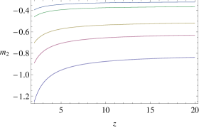
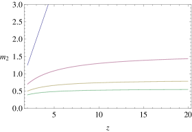
Here 2z+m12𝑧subscript𝑚12z+m_{1} is equivalent to z+n1𝑧𝑛1z+n-1 by using (3.1) and determines the scaling dimension of the dual operator. Note that the denominator of m2subscript𝑚2m_{2} must not be zero so as to ensure that the logarithmic term log2m2superscript2subscript𝑚2\log^{2-m_{2}} remains finite; recall that we want the slightly perturbed metric near the origin. Since (3.5) becomes singular when α~=z2(1+2z)~𝛼𝑧212𝑧\tilde{\alpha}=\frac{z}{2(-1+2z)}, where α~~𝛼\tilde{\alpha} decreases with increasing z𝑧z, approaching 1414\frac{1}{4} as z𝑧z\rightarrow\infty, we require α~14~𝛼14\tilde{\alpha}\leq\frac{1}{4}, where the equality is removed when z=𝑧z=\infty. This ensures m2subscript𝑚2m_{2} is finite for any z2𝑧2z\geq 2. In Fig.1, we depict m2subscript𝑚2m_{2} versus z𝑧z by varying α~~𝛼\tilde{\alpha}; we find that the value of m2subscript𝑚2m_{2} does not exceed 5454-\frac{5}{4} for |α~|<1~𝛼1|\tilde{\alpha}|<1 and any positive z𝑧z.

Refer to caption
(a) α~{1,1/2,3/10,1/4}~𝛼11231014\tilde{\alpha}\in\{-1,-1/2,-3/10,-1/4\}
Refer to caption
(b) α~{1/7,1/6,1/5,1/4}~𝛼17161514\tilde{\alpha}\in\{1/7,1/6,1/5,1/4\}
Figure 1: m2subscript𝑚2m_{2} versus z𝑧z for increasing values of α~~𝛼\tilde{\alpha} from bottom to top.

In (3.2)-(3.4), a new momentum scale ΛΛ\Lambda appears. We take it to be very small compared to the energy scale, where the Lifshitz spacetime lies. Thus ΛΛ\Lambda slightly deforms the Lifshitz spacetime and by doing so generates the marginally relevant mode; the pure Lifshitz spacetime solutions (2.27) are recovered when Λ0Λ0\Lambda\rightarrow 0. Furthermore we see from (3.2)-(3.4) that these solutions contain different modes due to the arbitrary parameters ξ𝜉\xi and ζ𝜁\zeta. This introduces an ambiguity related to defining the scale of ΛΛ\Lambda since the solution is invariant under the transformation

F(Λr;ζ,ξ;λ)=F(eλ/zΛr;e2λ(ζλξ),e2λξ;λ+λ)𝐹Λ𝑟𝜁𝜉𝜆𝐹superscript𝑒superscript𝜆𝑧Λ𝑟superscript𝑒2superscript𝜆𝜁superscript𝜆𝜉superscript𝑒2superscript𝜆𝜉𝜆superscript𝜆F(\Lambda r;\zeta,\xi;\lambda)=F(e^{\lambda^{\prime}/z}\Lambda r;e^{-2\lambda^{\prime}}(\zeta-\lambda^{\prime}\xi),e^{-2\lambda^{\prime}}\xi;\lambda+\lambda^{\prime}) (3.6)

where F𝐹F stands for k𝑘k, q𝑞q, and y𝑦y functions. We fix λ=0𝜆0\lambda=0 in (3.2)-(3.4) as in previous work where α~=0~𝛼0\tilde{\alpha}=0 Cheng:2009df and Park:2012bv .

By substituting (3.2)-(3.4) into the relation (2.22) and (2.23), the original functions f𝑓f and p𝑝p are obtained as

fl2𝑓superscript𝑙2\displaystyle\frac{f}{l^{2}} =F02log2m2m1z(rΛ)(rΛ)2z(11(z1)3(z+(24z)α~)3log(rΛ)(z3(7z4)+2z2(4z349z2+37z7)α~\displaystyle=F_{0}^{2}\frac{\log^{-2\frac{m_{2}}{m_{1}}z}(r\Lambda)}{(r\Lambda)^{2z}}\bigg{(}1-\frac{1}{(z-1)^{3}(z+(2-4z)\tilde{\alpha})^{3}\log(r\Lambda)}\bigg{(}z^{3}(7z-4)+2z^{2}(4z^{3}-49z^{2}+37z-7)\tilde{\alpha}
z(64z4487z3+406z2111z+8)α~2+2(89z5539z4+450z3131z2+7z+4)α~34(39z5\displaystyle-z(64z^{4}-487z^{3}+406z^{2}-111z+8)\tilde{\alpha}^{2}+2(89z^{5}-539z^{4}+450z^{3}-131z^{2}+7z+4)\tilde{\alpha}^{3}-4(39z^{5}
217z4+128z3+3z221z+8)α~4+8z2(z+1)(2z219z+11)α~5+(2z3(3z1)+4z2(z3\displaystyle-217z^{4}+128z^{3}+3z^{2}-21z+8)\tilde{\alpha}^{4}+8z^{2}(z+1)(2z^{2}-19z+11)\tilde{\alpha}^{5}+\bigg{(}2z^{3}(3z-1)+4z^{2}(z^{3}
21z2+12z2)α~2z(11z4199z3+137z233z+4)α~2+4(10z4213z3+157z243z+9)α~3\displaystyle-21z^{2}+12z-2)\tilde{\alpha}-2z(11z^{4}-199z^{3}+137z^{2}-33z+4)\tilde{\alpha}^{2}+4(10z^{4}-213z^{3}+157z^{2}-43z+9)\tilde{\alpha}^{3}
8(z497z3+63z211z+4)α~416z(2z3+9z28z+1)α~5)log(log(rΛ)))+),\displaystyle-8(z^{4}-97z^{3}+63z^{2}-11z+4)\tilde{\alpha}^{4}-16z(2z^{3}+9z^{2}-8z+1)\tilde{\alpha}^{5}\bigg{)}\log(-\log(r\Lambda))\bigg{)}+\cdots\bigg{)}, (3.7)
pl2𝑝superscript𝑙2\displaystyle\frac{p}{l^{2}} =P02log2m2m1(rΛ)(rΛ)2(1+1(z1)3(z+(24z)α~)3log(rΛ)(z2(5z2)+2z(3z338z2+24z\displaystyle=P_{0}^{2}\frac{\log^{2\frac{m_{2}}{m_{1}}}(r\Lambda)}{(r\Lambda)^{2}}\bigg{(}1+\frac{1}{(z-1)^{3}(z+(2-4z)\tilde{\alpha})^{3}\log(r\Lambda)}\bigg{(}z^{2}(5z-2)+2z(3z^{3}-38z^{2}+24z
4)α~(38z4377z3+280z269z+8)α~2+(82z4818z3+640z2178z+34)α~3(54z4\displaystyle-4)\tilde{\alpha}-(38z^{4}-377z^{3}+280z^{2}-69z+8)\tilde{\alpha}^{2}+(82z^{4}-818z^{3}+640z^{2}-178z+34)\tilde{\alpha}^{3}-(54z^{4}
732z3+504z292z+28)α~48(z+1)(2z3+17z215z+2)α~5+(2z2(3z1)+4z(z3\displaystyle-732z^{3}+504z^{2}-92z+28)\tilde{\alpha}^{4}-8(z+1)(2z^{3}+17z^{2}-15z+2)\tilde{\alpha}^{5}+\bigg{(}2z^{2}(3z-1)+4z(z^{3}
21z2+12z2)α~(22z4398z3+274z266z+8)α~2+4(10z4213z3+157z243z+9)α~3\displaystyle-21z^{2}+12z-2)\tilde{\alpha}-(22z^{4}-398z^{3}+274z^{2}-66z+8)\tilde{\alpha}^{2}+4(10z^{4}-213z^{3}+157z^{2}-43z+9)\tilde{\alpha}^{3}
8(z497z3+63z211z+4)α~416(z+1)(2z3+9z28z+1)α~5)log(log(rΛ)))+)\displaystyle-8(z^{4}-97z^{3}+63z^{2}-11z+4)\tilde{\alpha}^{4}-16(z+1)(2z^{3}+9z^{2}-8z+1)\tilde{\alpha}^{5}\bigg{)}\log(-\log(r\Lambda))\bigg{)}+\cdots\bigg{)} (3.8)

where F0subscript𝐹0F_{0} and P0subscript𝑃0P_{0} are integration constants. As we are assuming the Lifshitz spacetime in high energy regime, we introduce an arbitrary scale μ𝜇\mu

log(rΛ)=log(rμ)logμΛ,𝑟Λ𝑟𝜇𝜇Λ\log(r\Lambda)=\log(r\mu)-\log\frac{\mu}{\Lambda}, (3.9)

and expand the asymptotic solutions into UV regions where μΛmuch-greater-than𝜇Λ\mu\gg\Lambda

|1logμΛ|,|log(rμ)logμΛ|1,much-less-than1𝜇Λ𝑟𝜇𝜇Λ1\bigg{|}\frac{1}{\log\frac{\mu}{\Lambda}}\bigg{|},\qquad\bigg{|}\frac{\log(r\mu)}{\log\frac{\mu}{\Lambda}}\bigg{|}\ll 1, (3.10)

and then (3.7) and (3.8) become

f=𝑓absent\displaystyle f= 1r2z[1+1(z1)3(z(24z)α~)3log(μΛ)(z3(7z4+2z(z1)2log(rμ)+2(3z1)log(log(μΛ)))\displaystyle\frac{1}{r^{2z}}\bigg{[}1+\frac{1}{(z-1)^{3}(z-(2-4z)\tilde{\alpha})^{3}\log(\frac{\mu}{\Lambda})}\bigg{(}z^{3}\bigg{(}7z-4+2z(z-1)^{2}\log(r\mu)+2(3z-1)\log(\log(\frac{\mu}{\Lambda}))\bigg{)}
+2z2(4z349z2+37z7(11z3)z(z1)2log(rμ)+2(z321z2+12zz)log(log(μΛ)))α~2superscript𝑧24superscript𝑧349superscript𝑧237𝑧711𝑧3𝑧superscript𝑧12𝑟𝜇2superscript𝑧321superscript𝑧212𝑧𝑧𝜇Λ~𝛼\displaystyle+2z^{2}\bigg{(}4z^{3}-49z^{2}+37z-7-(11z-3)z(z-1)^{2}\log(r\mu)+2(z^{3}-21z^{2}+12z-z)\log(\log(\frac{\mu}{\Lambda}))\bigg{)}\tilde{\alpha}
z(64z4487z3+406z2111z+812z2(z1)2(7z3)log(rμ)+)α~2+)+],\displaystyle-z\bigg{(}64z^{4}-487z^{3}+406z^{2}-111z+8-12z^{2}(z-1)^{2}(7z-3)\log(r\mu)+\cdots\bigg{)}\tilde{\alpha}^{2}+\cdots\bigg{)}+\cdots\bigg{]}, (3.11)
p=𝑝absent\displaystyle p= 1r2[1(12α~)(z1)3(z(24z)α~)3log(μΛ)(z2(5z2+2z(z1)2log(rμ)+2(3z1)log(log(μΛ)))\displaystyle\frac{1}{r^{2}}\bigg{[}1-\frac{(1-2\tilde{\alpha})}{(z-1)^{3}(z-(2-4z)\tilde{\alpha})^{3}\log(\frac{\mu}{\Lambda})}\bigg{(}z^{2}\bigg{(}5z-2+2z(z-1)^{2}\log(r\mu)+2(3z-1)\log(\log(\frac{\mu}{\Lambda}))\bigg{)}
+2z(3z333z2+22z43z(z1)2(3z1)log(rμ)+2(z318z2+11z2)log(log(μΛ)))α~2𝑧3superscript𝑧333superscript𝑧222𝑧43𝑧superscript𝑧123𝑧1𝑟𝜇2superscript𝑧318superscript𝑧211𝑧2𝜇Λ~𝛼\displaystyle+2z\bigg{(}3z^{3}-33z^{2}+22z-4-3z(z-1)^{2}(3z-1)\log(r\mu)+2(z^{3}-18z^{2}+11z-2)\log(\log(\frac{\mu}{\Lambda}))\bigg{)}\tilde{\alpha}
(26z4245z3+192z253z+824z2(z1)2(2z1)log(rμ)+)α~2+)+]\displaystyle-\bigg{(}26z^{4}-245z^{3}+192z^{2}-53z+8-24z^{2}(z-1)^{2}(2z-1)\log(r\mu)+\cdots\bigg{)}\tilde{\alpha}^{2}+\cdots\bigg{)}+\cdots\bigg{]} (3.12)

where the t𝑡t and x𝑥x coordinates are rescaled by

t(Λlogm2m1(μΛ))z1F0t,xΛlogm2m1(μΛ)1P0x.formulae-sequence𝑡superscriptΛsuperscriptsubscript𝑚2subscript𝑚1𝜇Λ𝑧1subscript𝐹0𝑡𝑥Λsuperscriptsubscript𝑚2subscript𝑚1𝜇Λ1subscript𝑃0𝑥\displaystyle t\rightarrow\bigg{(}\Lambda\log^{\frac{m_{2}}{m_{1}}}\bigg{(}\frac{\mu}{\Lambda}\bigg{)}\bigg{)}^{z}\frac{1}{F_{0}}t,\;\;\;\;\;\;x\rightarrow\frac{\Lambda}{\log^{\frac{m_{2}}{m_{1}}}(\frac{\mu}{\Lambda})}\frac{1}{P_{0}}x. (3.13)

4.  Holographic Renormalization

As we are considering the spacetime at finite temperature, the action is related to the free energy via

F=Tlog𝒵=TSϵ(g)𝐹𝑇𝒵𝑇subscript𝑆italic-ϵsubscript𝑔F=-T\log{\mathcal{Z}}=TS_{\epsilon}(g_{*}) (4.1)

where Sϵsubscript𝑆italic-ϵS_{\epsilon} and gsubscript𝑔g_{*} indicate the Euclidean action and metric respectively. At the asymptotic boundary near r0𝑟0r\rightarrow 0, the action includes a boundary term to yield the bulk equations of motion

Sϵ=Sbulk,ϵ+Sboundary,ϵsubscript𝑆italic-ϵsubscript𝑆bulkitalic-ϵsubscript𝑆boundaryitalic-ϵS_{\epsilon}=S_{\textrm{bulk},\epsilon}+S_{\textrm{boundary},\epsilon} (4.2)

where each term is

Sbulk,ϵsubscript𝑆bulkitalic-ϵ\displaystyle S_{\textrm{bulk},\epsilon} =dn+1xg(12κn+12[R+2Λ~+αGB]1gv2[14H2+γ2B2]),absentsuperscript𝑑𝑛1𝑥𝑔12superscriptsubscript𝜅𝑛12delimited-[]𝑅2~Λ𝛼subscript𝐺𝐵1superscriptsubscript𝑔𝑣2delimited-[]14superscript𝐻2𝛾2superscript𝐵2\displaystyle=\int d^{n+1}x\sqrt{g}\bigg{(}\frac{1}{2\kappa_{n+1}^{2}}[R+2\tilde{\Lambda}+\alpha\mathcal{L}_{GB}]-\frac{1}{{g_{v}}^{2}}\bigg{[}\frac{1}{4}H^{2}+\frac{\gamma}{2}B^{2}\bigg{]}\bigg{)},
Sboundary,ϵsubscript𝑆boundaryitalic-ϵ\displaystyle S_{\textrm{boundary},\epsilon} =1κn+12Σdnxγ(K+2α(J2G^abKab))absent1superscriptsubscript𝜅𝑛12subscriptΣsuperscript𝑑𝑛𝑥𝛾𝐾2𝛼𝐽2superscript^𝐺𝑎𝑏subscript𝐾𝑎𝑏\displaystyle=\frac{1}{\kappa_{n+1}^{2}}\int_{\Sigma}d^{n}x\sqrt{\gamma}\bigg{(}K+2\alpha(J-2\hat{G}^{ab}K_{ab})\bigg{)} (4.3)

and where G^absuperscript^𝐺𝑎𝑏\hat{G}^{ab} is the n𝑛n-dimensional Einstein tensor on ΣΣ\Sigma corresponding to γabsubscript𝛾𝑎𝑏\gamma_{ab} and J=Jabγab𝐽subscript𝐽𝑎𝑏superscript𝛾𝑎𝑏J=J_{ab}\gamma^{ab}, with

Jab=13(2KKacKbc+KcdKcdKab2KacKcdKdbK2Kab).subscript𝐽𝑎𝑏132𝐾subscript𝐾𝑎𝑐subscriptsuperscript𝐾𝑐𝑏subscript𝐾𝑐𝑑superscript𝐾𝑐𝑑subscript𝐾𝑎𝑏2subscript𝐾𝑎𝑐superscript𝐾𝑐𝑑subscript𝐾𝑑𝑏superscript𝐾2subscript𝐾𝑎𝑏J_{ab}=\frac{1}{3}(2KK_{ac}K^{c}_{\;\;b}+K_{cd}K^{cd}K_{ab}-2K_{ac}K^{cd}K_{db}-K^{2}K_{ab}). (4.4)

Defining F=dn1x𝐹superscript𝑑𝑛1𝑥F=\int d^{n-1}x\;\mathcal{F}, the free energy density \mathcal{F}, which is the free energy density per unit (n1)𝑛1(n-1)-dimensional spatial volume, is

bulksubscriptbulk\displaystyle{\mathcal{F}}_{\textrm{bulk}} =ln12κn+12limr0rf(r)p(r)p(r)n32(1α(n2)r2l2p(r)p(r)((n3)2p(r)p(r)+f(r)f(r))),absentsuperscript𝑙𝑛12superscriptsubscript𝜅𝑛12subscript𝑟0𝑟𝑓𝑟superscript𝑝𝑟𝑝superscript𝑟𝑛321𝛼𝑛2superscript𝑟2superscript𝑙2superscript𝑝𝑟𝑝𝑟𝑛32superscript𝑝𝑟𝑝𝑟superscript𝑓𝑟𝑓𝑟\displaystyle=-\frac{l^{n-1}}{2\kappa_{n+1}^{2}}\lim_{r\rightarrow 0}r\sqrt{f(r)}p^{\prime}(r)p(r)^{\frac{n-3}{2}}\bigg{(}1-\alpha\frac{(n-2)r^{2}}{l^{2}}\frac{p^{\prime}(r)}{p(r)}\bigg{(}\frac{(n-3)}{2}\frac{p^{\prime}(r)}{p(r)}+\frac{f^{\prime}(r)}{f(r)}\bigg{)}\bigg{)},
boundarysubscriptboundary\displaystyle{\mathcal{F}}_{\textrm{boundary}} =ln1κn+12limr0(r(f(r)p(r)n12)α(n1)(n2)r36l2p(r)2f(r)p(r)(f(r)3p(r)n32)).absentsuperscript𝑙𝑛1superscriptsubscript𝜅𝑛12subscript𝑟0𝑟superscript𝑓𝑟𝑝superscript𝑟𝑛12𝛼𝑛1𝑛2superscript𝑟36superscript𝑙2superscript𝑝superscript𝑟2𝑓𝑟𝑝𝑟superscript3𝑓𝑟𝑝superscript𝑟𝑛32\displaystyle=\frac{l^{n-1}}{\kappa_{n+1}^{2}}\lim_{r\rightarrow 0}\bigg{(}r\bigg{(}\sqrt{f(r)}p(r)^{\frac{n-1}{2}}\bigg{)}^{\prime}-\alpha\frac{(n-1)(n-2)r^{3}}{6l^{2}}\frac{p^{\prime}(r)^{2}}{f(r)p(r)}\bigg{(}\sqrt[3]{f(r)}p(r)^{\frac{n-3}{2}}\bigg{)}^{\prime}\bigg{)}. (4.5)

Considering the boundary of the spacetime near r0𝑟0r\rightarrow 0, these quantities are divergent upon insertion of (3) - (3.12), and so counterterms are required to render them finite. These counterterms also should be constructed so as to preserve the covariance of the action at the boundary and to yield a well-defined variational principle. To meet the first condition, one convenient option would be to employ B2=BμBμsuperscript𝐵2superscript𝐵𝜇subscript𝐵𝜇B^{2}=B^{\mu}B_{\mu} and to consider a functional of this quantity on the boundary, which could be any form if canceling divergences were the only criterion. We take the counterterms to be the combination C0+C1B2+C2B4+subscript𝐶0subscript𝐶1superscript𝐵2subscript𝐶2superscript𝐵4C_{0}+C_{1}B^{2}+C_{2}B^{4}+\cdots and then replace B2superscript𝐵2B^{2} with κn+12gv2B2(z1)(12α~)zsubscriptsuperscript𝜅2𝑛1subscriptsuperscript𝑔2𝑣superscript𝐵2𝑧112~𝛼𝑧-\frac{\kappa^{2}_{n+1}}{g^{2}_{v}}B^{2}-\frac{(z-1)(1-2\tilde{\alpha})}{z}, because the counterterms should vanish for the pure Lifshitz spacetime.

The counterterms are precisely expressed by

c.tsubscriptc.t\displaystyle{\mathcal{F}}_{\textrm{c.t}} =ln12κn+12limr0f(r)p(r)n12(j=02Cj(κn+12gv2B2(z1)(12α~)z)j)absentsuperscript𝑙𝑛12superscriptsubscript𝜅𝑛12subscript𝑟0𝑓𝑟𝑝superscript𝑟𝑛12subscriptsuperscript2𝑗0subscript𝐶𝑗superscriptsubscriptsuperscript𝜅2𝑛1subscriptsuperscript𝑔2𝑣superscript𝐵2𝑧112~𝛼𝑧𝑗\displaystyle=\frac{l^{n-1}}{2\kappa_{n+1}^{2}}\lim_{r\rightarrow 0}\sqrt{f(r)}p(r)^{\frac{n-1}{2}}\bigg{(}\sum^{2}_{j=0}C_{j}\bigg{(}-\frac{\kappa^{2}_{n+1}}{g^{2}_{v}}B^{2}-\frac{(z-1)(1-2\tilde{\alpha})}{z}\bigg{)}^{j}\bigg{)}
=ln12κn+12limr0f(r)p(r)n12(j=02Cj(k(r)2(z1)(12α~)z)j)absentsuperscript𝑙𝑛12superscriptsubscript𝜅𝑛12subscript𝑟0𝑓𝑟𝑝superscript𝑟𝑛12subscriptsuperscript2𝑗0subscript𝐶𝑗superscript𝑘superscript𝑟2𝑧112~𝛼𝑧𝑗\displaystyle=\frac{l^{n-1}}{2\kappa_{n+1}^{2}}\lim_{r\rightarrow 0}\sqrt{f(r)}p(r)^{\frac{n-1}{2}}\bigg{(}\sum^{2}_{j=0}C_{j}\bigg{(}k(r)^{2}-\frac{(z-1)(1-2\tilde{\alpha})}{z}\bigg{)}^{j}\bigg{)} (4.6)

where the Cjsubscript𝐶𝑗C_{j} are not constants but rather series in 1/log(rΛ)1𝑟Λ1/\log(r\Lambda), which expand similarly to (3.2) - (3.4). Thus the free energy density is finally written as

=absent\displaystyle{\mathcal{F}}= bulk+boundary+c.tsubscriptbulksubscriptboundarysubscriptc.t\displaystyle{\mathcal{F}}_{\textrm{bulk}}+{\mathcal{F}}_{\textrm{boundary}}+{\mathcal{F}}_{\textrm{c.t}}
=\displaystyle= ln12κn+12limr0f(r)p(r)n12((n2)rp(r)p(r)+rf(r)f(r)+α~(r32f(r)f(r)p(r)2p(r)2(n4)6r3p(r)3p(r)3)\displaystyle\frac{l^{n-1}}{2\kappa_{n+1}^{2}}\lim_{r\rightarrow 0}\sqrt{f(r)}p(r)^{\frac{n-1}{2}}\bigg{(}\frac{(n-2)rp^{\prime}(r)}{p(r)}+\frac{rf^{\prime}(r)}{f(r)}+\tilde{\alpha}\bigg{(}-\frac{r^{3}}{2}\frac{f^{\prime}(r)}{f(r)}\frac{p^{\prime}(r)^{2}}{p(r)^{2}}-\frac{(n-4)}{6}\frac{r^{3}p^{\prime}(r)^{3}}{p(r)^{3}}\bigg{)}
+j=02Cj(k(r)2(z1)(12α~)z)j).\displaystyle+\sum^{2}_{j=0}C_{j}\bigg{(}k(r)^{2}-\frac{(z-1)(1-2\tilde{\alpha})}{z}\bigg{)}^{j}\bigg{)}. (4.7)

The counterterms also yield a well-defined variational principle of the on-shell action; this process defines the boundary stress tensor, which yields the conserved quantities. Here we obtain some physical quantities such as energy density \mathcal{E}, pressure 𝒫𝒫\mathcal{P}, and flow 𝒥isuperscript𝒥𝑖\mathcal{J}^{i} by finding the boundary stress tensor. To do this we start with the variation of the action known as

δ=γ2τabδγab+𝒥aδBa𝛿𝛾2superscript𝜏𝑎𝑏𝛿subscript𝛾𝑎𝑏superscript𝒥𝑎𝛿subscript𝐵𝑎\delta{\mathcal{F}}=\frac{\sqrt{\gamma}}{2}\tau^{ab}\delta\gamma_{ab}+\mathcal{J}^{a}\delta B_{a} (4.8)

where τabsuperscript𝜏𝑎𝑏\tau^{ab} contributes to yield conserved quantities via

Q=dn1xσξakbτab𝑄superscript𝑑𝑛1𝑥𝜎subscript𝜉𝑎subscript𝑘𝑏superscript𝜏𝑎𝑏Q=-\int d^{n-1}x\sqrt{\sigma}\xi_{a}k_{b}\tau^{ab} (4.9)

where σ=σx1x1σxn1xn1𝜎subscript𝜎subscript𝑥1subscript𝑥1subscript𝜎subscript𝑥𝑛1subscript𝑥𝑛1\sqrt{\sigma}=\sqrt{\sigma_{x_{1}x_{1}}\cdots\sigma_{x_{n-1}x_{n-1}}} is the spatial volume element, ξasubscript𝜉𝑎\xi_{a} are boundary Killing fields, and kasubscript𝑘𝑎k_{a} is the unit vector normal to the boundary surface. In the presence of the non-scalar fields, the boundary stress tensor τabsuperscript𝜏𝑎𝑏\tau^{ab} should be modified to include the contribution of the massive vector fields. To do so, we employ the vielbein frame at the boundary of the metric

γab=ηa^b^eaa^ebb^,η=diag(±1,1,1,)formulae-sequencesubscript𝛾𝑎𝑏subscript𝜂^𝑎^𝑏subscriptsuperscript𝑒^𝑎𝑎subscriptsuperscript𝑒^𝑏𝑏𝜂diagplus-or-minus111\gamma_{ab}=\eta_{\hat{a}\hat{b}}e^{\hat{a}}_{a}e^{\hat{b}}_{b},\;\;\;\eta=\textrm{diag}(\pm 1,1,1,\cdots) (4.10)

where

et^=eat^dxa=fdτ,exi^=pdxi.formulae-sequencesuperscript𝑒^𝑡subscriptsuperscript𝑒^𝑡𝑎𝑑superscript𝑥𝑎𝑓𝑑𝜏superscript𝑒^subscript𝑥𝑖𝑝𝑑subscript𝑥𝑖e^{\hat{t}}=e^{\hat{t}}_{a}dx^{a}=\sqrt{f}d\tau,\;\;\;\;e^{\hat{x_{i}}}=\sqrt{p}\;dx_{i}. (4.11)

Then (4.8) is rewritten with the new boundary stress tensor 𝒯absuperscript𝒯𝑎𝑏\mathcal{T}^{ab}

δ=γ𝒯a^aδeaa^+𝒥a^δBa^𝛿𝛾subscriptsuperscript𝒯𝑎^𝑎𝛿subscriptsuperscript𝑒^𝑎𝑎superscript𝒥^𝑎𝛿subscript𝐵^𝑎\delta\mathcal{F}=\sqrt{\gamma}\;\mathcal{T}^{a}_{\;\;\hat{a}}\delta e^{\hat{a}}_{a}+\mathcal{J}^{\hat{a}}\delta B_{\hat{a}} (4.12)

where

𝒯ab=Ta^aeba^,𝒯ab=τab+1γ𝒥(aBb).\mathcal{T}^{ab}=T^{a}_{\;\;\hat{a}}e^{b\hat{a}},\qquad\mathcal{T}^{ab}=\tau^{ab}+\frac{1}{\sqrt{\gamma}}\mathcal{J}^{(a}B^{b)}. (4.13)

The energy density is expressed as

=σkaξbTab=γτtt+𝒥tBt𝜎subscript𝑘𝑎subscript𝜉𝑏superscript𝑇𝑎𝑏𝛾subscriptsuperscript𝜏𝑡𝑡superscript𝒥𝑡subscript𝐵𝑡\mathcal{E}=\sqrt{\sigma}k_{a}\xi_{b}T^{ab}=\sqrt{\gamma}\tau^{t}_{\;\;t}+\mathcal{J}^{t}B_{t} (4.14)

and the pressure is given by

𝒫=γτxx.𝒫𝛾subscriptsuperscript𝜏𝑥𝑥\mathcal{P}=-\sqrt{\gamma}\tau^{x}_{\;\;x}. (4.15)

From the variation of the action (4.2)-(4.4) with respect to γabsubscript𝛾𝑎𝑏\gamma_{ab}, we obtain for τabsuperscript𝜏𝑎𝑏\tau^{ab} the expression

τab=2γδδγab=1κn+12[(KγabKab)+2α(Jγab3Jab2P^acdbKcd)\displaystyle\tau^{ab}=\frac{2}{\sqrt{\gamma}}\frac{\delta{\mathcal{F}}}{\delta\gamma_{ab}}=\frac{1}{\kappa_{n+1}^{2}}\bigg{[}(K\gamma^{ab}-K^{ab})+2\alpha(J\gamma^{ab}-3J^{ab}-2\hat{P}^{acdb}K_{cd})
+12lj=02Cj(γab(κn+12gv2B2(z1)(12α~)z)j+2jκn+12gv2BaBb(κn+12gv2B2(z1)(12α~)z)j1)]\displaystyle+\frac{1}{2l}\sum^{2}_{j=0}C_{j}\bigg{(}\gamma^{ab}\bigg{(}-\frac{\kappa_{n+1}^{2}}{{g_{v}}^{2}}{B}^{2}-\frac{(z-1)(1-2\tilde{\alpha})}{z}\bigg{)}^{j}+\frac{2j{\kappa_{n+1}}^{2}}{{g_{v}}^{2}}{B}^{a}{B}^{b}\bigg{(}-\frac{\kappa_{n+1}^{2}}{{g_{v}}^{2}}{B}^{2}-\frac{(z-1)(1-2\tilde{\alpha})}{z}\bigg{)}^{j-1}\bigg{)}\bigg{]} (4.16)

where

P^abcd=R^abcd+2R^b[cgd]a2R^a[cgd]b+R^ga[cgd]b,\hat{P}_{abcd}=\hat{R}_{abcd}+2\hat{R}_{b[c}g_{d]a}-2\hat{R}_{a[c}g_{d]b}+\hat{R}g_{a[c}g_{d]b}, (4.17)

in which the R^^𝑅\hat{R}’s are various contractions of Riemann tensors defined on the n𝑛n-dimensional hypersurface associated with γabsubscript𝛾𝑎𝑏\gamma_{ab}. From the variation of the action with respect to the vector field strength Btsubscript𝐵𝑡B_{t}, 𝒥t^superscript𝒥^𝑡{\mathcal{J}}^{\hat{t}} we obtain

𝒥t^=superscript𝒥^𝑡absent\displaystyle{\mathcal{J}}^{\hat{t}}= f(r)δSδBt,𝑓𝑟𝛿𝑆𝛿subscript𝐵𝑡\displaystyle\sqrt{f(r)}\frac{\delta S}{\delta B_{t}},
=\displaystyle= ln2gvκn+1limr0f(r)p(r)n12(r(k(r)f(r))f(r)+k(r)j=02jCj(k(r)2(z1)(12α~)z)j1)superscript𝑙𝑛2subscript𝑔𝑣subscript𝜅𝑛1subscript𝑟0𝑓𝑟𝑝superscript𝑟𝑛12𝑟superscript𝑘𝑟𝑓𝑟𝑓𝑟𝑘𝑟subscriptsuperscript2𝑗0𝑗subscript𝐶𝑗superscript𝑘superscript𝑟2𝑧112~𝛼𝑧𝑗1\displaystyle\frac{l^{n-2}}{g_{v}\kappa_{n+1}}\lim_{r\rightarrow 0}\sqrt{f(r)}p(r)^{\frac{n-1}{2}}\bigg{(}\frac{r(k(r)\sqrt{f(r)})^{\prime}}{\sqrt{f(r)}}+k(r)\sum^{2}_{j=0}jC_{j}\bigg{(}k(r)^{2}-\frac{(z-1)(1-2\tilde{\alpha})}{z}\bigg{)}^{j-1}\bigg{)}
=\displaystyle= ln2gvκn+1limr0f(r)p(r)n12(12y(r)+k(r)j=02jCj(k(r)2(z1)(12α~)z)j1)superscript𝑙𝑛2subscript𝑔𝑣subscript𝜅𝑛1subscript𝑟0𝑓𝑟𝑝superscript𝑟𝑛1212𝑦𝑟𝑘𝑟subscriptsuperscript2𝑗0𝑗subscript𝐶𝑗superscript𝑘superscript𝑟2𝑧112~𝛼𝑧𝑗1\displaystyle\frac{l^{n-2}}{g_{v}\kappa_{n+1}}\lim_{r\rightarrow 0}\sqrt{f(r)}p(r)^{\frac{n-1}{2}}\bigg{(}-\frac{1}{2}y(r)+k(r)\sum^{2}_{j=0}jC_{j}\bigg{(}k(r)^{2}-\frac{(z-1)(1-2\tilde{\alpha})}{z}\bigg{)}^{j-1}\bigg{)} (4.18)

where other components of 𝒥a^superscript𝒥^𝑎{\mathcal{J}}^{\hat{a}} vanish. Then the energy density becomes

=absent\displaystyle\mathcal{E}= ln12κn+12limr0f(r)p(r)n12[(n1)rp(r)p(r)k(r)y(r)+α~((n1)6r3p(r)3p(r)3)\displaystyle\frac{l^{n-1}}{2\kappa_{n+1}^{2}}\lim_{r\rightarrow 0}\sqrt{f(r)}p(r)^{\frac{n-1}{2}}\bigg{[}(n-1)\frac{rp^{\prime}(r)}{p(r)}-k(r)y(r)+\tilde{\alpha}\bigg{(}-\frac{(n-1)}{6}\frac{r^{3}p^{\prime}(r)^{3}}{p(r)^{3}}\bigg{)}
+j=02Cj(k(r)2(z1)(12α~)z)j],\displaystyle+\sum^{2}_{j=0}C_{j}\bigg{(}k(r)^{2}-\frac{(z-1)(1-2\tilde{\alpha})}{z}\bigg{)}^{j}\bigg{]}, (4.19)

and the pressure takes the same form of the free energy density with the opposite sign

𝒫=.𝒫\mathcal{P}=-\mathcal{F}. (4.20)

To ensure a finite value of the action and a well-defined variational principle δS=0𝛿𝑆0\delta S=0, we expect our counterterms (4.6) to render the free energy density (4.7), the flow (4.18), and the energy density (4.19) finite when r0𝑟0r\rightarrow 0. Expanding these functions with the asymptotic solution (3.2)-(3.4), they take the form

F1rz+n1(F1[1log(rΛ)]+(rΛ)z+n1log2m2(rΛ)(F2[1log(rΛ)]+))+countertermssimilar-to𝐹1superscript𝑟𝑧𝑛1subscript𝐹1delimited-[]1𝑟Λsuperscript𝑟Λ𝑧𝑛1superscript2subscript𝑚2𝑟Λsubscript𝐹2delimited-[]1𝑟ΛcountertermsF\sim\frac{1}{r^{z+n-1}}\bigg{(}F_{1}[\frac{1}{\log(r\Lambda)}]+\cdots(r\Lambda)^{z+n-1}\log^{2-m_{2}}(r\Lambda)\bigg{(}F_{2}[\frac{1}{\log(r\Lambda)}]+\cdots\bigg{)}\bigg{)}+\textrm{counterterms} (4.21)

where F𝐹F stands for \mathcal{F}, \mathcal{E}, and 𝒥t^superscript𝒥^𝑡\mathcal{J}^{\hat{t}}, and F1subscript𝐹1F_{1} and F2subscript𝐹2F_{2} indicate the parts involving series of log(rΛ)𝑟Λ\log(r\Lambda) in the expression of \mathcal{F}, \mathcal{E}, and 𝒥t^superscript𝒥^𝑡\mathcal{J}^{\hat{t}}. As shown in (4.21), divergences occur as r0𝑟0r\rightarrow 0. The divergences due to 1rz+n11superscript𝑟𝑧𝑛1\frac{1}{r^{z+n-1}} are eliminated by the two coefficients C0subscript𝐶0C_{0} and C1subscript𝐶1C_{1}, expanded as a series in 1/log(rΛ)1𝑟Λ1/\log(r\Lambda). To prevent divergences due to log2m2(rΛ)superscript2subscript𝑚2𝑟Λ\log^{2-m_{2}}(r\Lambda), another coefficient C2subscript𝐶2C_{2} is required. Then C0subscript𝐶0C_{0}, C1subscript𝐶1C_{1}, and C2subscript𝐶2C_{2} become

C0=subscript𝐶0absent\displaystyle C_{0}= 2(3+6z+(614z)α~+4(2+3z)α~2)3+6α~+2(z2α~)(1+2(2+z)α~)(z+(1+z)α~)3(z1)3(2z1)(z+(24z)α~)2log2(rΛ)236𝑧614𝑧~𝛼423𝑧superscript~𝛼236~𝛼2𝑧2~𝛼122𝑧~𝛼superscript𝑧1𝑧~𝛼3superscript𝑧132𝑧1superscript𝑧24𝑧~𝛼2superscript2𝑟Λ\displaystyle-\frac{2(-3+6z+(6-14z)\tilde{\alpha}+4(-2+3z)\tilde{\alpha}^{2})}{-3+6\tilde{\alpha}}+\frac{2(z-2\tilde{\alpha})(1+2(-2+z)\tilde{\alpha})(-z+(1+z)\tilde{\alpha})^{3}}{(z-1)^{3}(2z-1)(z+(2-4z)\tilde{\alpha})^{2}\log^{2}(r\Lambda)}
+(z(1+z)α~)23(2z1)2(z1)5(z+(24z)α~3)log3(rΛ)(3z(12z3z2+2z3+4z4)+(321z\displaystyle+\frac{(z-(1+z)\tilde{\alpha})^{2}}{3(2z-1)^{2}(z-1)^{5}(z+(2-4z)\tilde{\alpha}^{3})\log^{3}(r\Lambda)}\bigg{(}3z(1-2z-3z^{2}+2z^{3}+4z^{4})+(-3-21z
+109z2+33z3146z448z5+16z6)α~+)+,\displaystyle+109z^{2}+33z^{3}-146z^{4}-48z^{5}+16z^{6})\tilde{\alpha}+\cdots\bigg{)}+\cdots, (4.22)
C1=subscript𝐶1absent\displaystyle C_{1}= z2z(z2α~)(z(1+z)α~)2(z1)2(2z1)(2α~1)(z+(24z)α~)log(rΛ)𝑧2𝑧𝑧2~𝛼superscript𝑧1𝑧~𝛼2superscript𝑧122𝑧12~𝛼1𝑧24𝑧~𝛼𝑟Λ\displaystyle z-\frac{2z(z-2\tilde{\alpha})(z-(1+z)\tilde{\alpha})^{2}}{(z-1)^{2}(2z-1)(2\tilde{\alpha}-1)(z+(2-4z)\tilde{\alpha})\log(r\Lambda)}
z(z+(1+z)α~)2(2z1)2(z1)4(2α~1)(z+(24z)α~)2log2(rΛ)(z(310zz2+14z3)+(39z\displaystyle-\frac{z(-z+(1+z)\tilde{\alpha})}{2(2z-1)^{2}(z-1)^{4}(2\tilde{\alpha}-1)(z+(2-4z)\tilde{\alpha})^{2}\log^{2}(r\Lambda)}\bigg{(}z(3-10z-z^{2}+14z^{3})+(-3-9z
+113z2103z370z4+24z5)α~+)+,\displaystyle+113z^{2}-103z^{3}-70z^{4}+24z^{5})\tilde{\alpha}+\cdots\bigg{)}+\cdots, (4.23)
C2=subscript𝐶2absent\displaystyle C_{2}= z2(13z+4zα~)4(z1)(2z1)(2α~1)2+z24(2z1)2(z1)3(2α~1)2(z+(24z)α~)log(rΛ)(z(314z\displaystyle\frac{z^{2}(1-3z+4z\tilde{\alpha})}{4(z-1)(2z-1)(2\tilde{\alpha}-1)^{2}}+\frac{z^{2}}{4(2z-1)^{2}(z-1)^{3}(2\tilde{\alpha}-1)^{2}(z+(2-4z)\tilde{\alpha})\log(r\Lambda)}\bigg{(}z(3-14z
+15z2)+(3+3z+65z2119z3+30z4)α~+)+Δlog2(rΛ)\displaystyle+15z^{2})+(-3+3z+65z^{2}-119z^{3}+30z^{4})\tilde{\alpha}+\cdots\bigg{)}+\frac{\Delta}{\log^{2}(r\Lambda)}
+z2log(log(rΛ))4(12z)2(1+z)5(12α~2(z+(1+z)α~)(z+(2+4z)α~)3log2(rΛ)\displaystyle+\frac{z^{2}\log(-\log(r\Lambda))}{4(1-2z)^{2}(-1+z)^{5}(1-2\tilde{\alpha}^{2}(-z+(1+z)\tilde{\alpha})(-z+(-2+4z)\tilde{\alpha})^{3}\log^{2}(r\Lambda)}
×((13z)2z3(3+5z)+z2(9+110z532z2+1154z3955z4+120z5)α~+).absentsuperscript13𝑧2superscript𝑧335𝑧superscript𝑧29110𝑧532superscript𝑧21154superscript𝑧3955superscript𝑧4120superscript𝑧5~𝛼\displaystyle\times\bigg{(}(1-3z)^{2}z^{3}(-3+5z)+z^{2}(-9+110z-532z^{2}+1154z^{3}-955z^{4}+120z^{5})\tilde{\alpha}+\cdots\bigg{)}. (4.24)

where C0subscript𝐶0C_{0} and C1subscript𝐶1C_{1} keep expanding with infinite series of 1/log(rΛ)1𝑟Λ1/\log(r\Lambda) as the asymptotic solutions expand. However C2subscript𝐶2C_{2} just consists of a finite number of terms, because the log2m2(rΛ)superscript2subscript𝑚2𝑟Λ\log^{2-m_{2}}(r\Lambda) quantity in (4.21) is divided by 1/logi(rΛ)1superscript𝑖𝑟Λ1/\log^{i}(r\Lambda) (where i=1,2,𝑖12i=1,2,\cdots) from F2subscript𝐹2F_{2} and so when i𝑖i becomes 2m22subscript𝑚22-m_{2} divergences due to log2m2(rΛ)superscript2subscript𝑚2𝑟Λ\log^{2-m_{2}}(r\Lambda) vanish. These solutions, however, have an ambiguity ΔΔ\Delta as shown in (4.24). It turns out that ΔΔ\Delta does not affect numerical work for the free energy density and the energy density, as we shall show in the next section.

Inserting the solution (4.22)-(4.24) into (4.7), (4.18), and (4.19), we find

=absent\displaystyle\mathcal{F}= ln1κn+12z(z1)(12α~)((z(z+1)α~)ζ+X(2z1)(z1)2(z(2+4z)α~)3ξ),superscript𝑙𝑛1subscriptsuperscript𝜅2𝑛1𝑧𝑧112~𝛼𝑧𝑧1~𝛼𝜁𝑋2𝑧1superscript𝑧12superscript𝑧24𝑧~𝛼3𝜉\displaystyle\frac{l^{n-1}}{\kappa^{2}_{n+1}}\frac{\sqrt{z}}{\sqrt{(z-1)(1-2\tilde{\alpha})}}\bigg{(}(z-(z+1)\tilde{\alpha})\zeta+\frac{X}{(2z-1)(z-1)^{2}(z-(-2+4z)\tilde{\alpha})^{3}}\xi\bigg{)}, (4.25)
=absent\displaystyle\mathcal{E}= ln1κn+12(z2α~)(z1)z(2z1)(12α~)3/2((z(z+1)α~)ζY(2z1)(z1)2(z(2+4z)α~)3ξ),superscript𝑙𝑛1subscriptsuperscript𝜅2𝑛1𝑧2~𝛼𝑧1𝑧2𝑧1superscript12~𝛼32𝑧𝑧1~𝛼𝜁𝑌2𝑧1superscript𝑧12superscript𝑧24𝑧~𝛼3𝜉\displaystyle-\frac{l^{n-1}}{\kappa^{2}_{n+1}}\frac{(z-2\tilde{\alpha})}{\sqrt{(z-1)z}(2z-1)(1-2\tilde{\alpha})^{3/2}}\bigg{(}(z-(z+1)\tilde{\alpha})\zeta-\frac{Y}{(2z-1)(z-1)^{2}(z-(-2+4z)\tilde{\alpha})^{3}}\xi\bigg{)}, (4.26)
𝒥t^=superscript𝒥^𝑡absent\displaystyle\mathcal{J}^{\hat{t}}= 1gvln2κn+11(12z)2(12α~)2((z1)(z2α~)α~ζ+4(z1)(12α)3Δzξ\displaystyle\frac{1}{g_{v}}\frac{l^{n-2}}{\kappa_{n+1}}\frac{1}{(1-2z)^{2}(1-2\tilde{\alpha})^{2}}\bigg{(}-(z-1)(z-2\tilde{\alpha})\tilde{\alpha}\;\zeta+\frac{4(z-1)(1-2\alpha)^{3}\Delta}{z}\xi
+Z2(z1)4(12z)(z(1+z)α~)(z(2+4z)α~)3ξ),\displaystyle+\frac{Z}{2(z-1)^{4}(1-2z)(z-(1+z)\tilde{\alpha})(z-(-2+4z)\tilde{\alpha})^{3}}\xi\bigg{)}, (4.27)

where X𝑋X, Y𝑌Y, and Z𝑍Z are functions of z𝑧z and α~~𝛼\tilde{\alpha}, and are displayed in (A). This result implies for the pure Lifshitz spacetime to be

==𝒥t^=0,superscript𝒥^𝑡0\mathcal{F}=\mathcal{E}=\mathcal{J}^{\hat{t}}=0, (4.28)

since ζ=ξ=0𝜁𝜉0\zeta=\xi=0 for the pure Lifshitz solution.

5.  Finite Temperature

We have so far worked near boundary of the spacetime. We now move to the near-horizon region of a black hole. In this section, we first obtain (planar) black hole solutions expanded near the horizon, and find some thermodynamic quantities such as temperature T𝑇T, entropy density s𝑠s, horizon flux density of the massive vector field ϕitalic-ϕ\phi at near horizon r=r+𝑟subscript𝑟r=r_{+}. Then we prove the integrated first law by constructing an RG-invariant quantity K¯¯𝐾\bar{K}. We find analytic expressions for 0Tssubscript0𝑇𝑠\frac{\mathcal{F}_{0}}{Ts} and 0Tssubscript0𝑇𝑠\frac{\mathcal{E}_{0}}{Ts} when the marginally relevant modes are turned off. In subsequent sections we check these relationships numerically and find agreement in all dimensions we study.

5.1  Expansion and Physical quantities near the horizon

Let us consider a black hole solution defined by f(r+)=0𝑓subscript𝑟0f(r_{+})=0, and expand the solution near horizon r=r+𝑟subscript𝑟r=r_{+}. The expansions in powers of (1rr+)1𝑟subscript𝑟(1-\frac{r}{r_{+}}) are determined by equation of motion (2.19)-(2.21). We find

f(r)𝑓𝑟\displaystyle f(r) =f0((1rr+)2+(1rr+)3+112(12α~)2(z2α~)2(z(8h02(2+3z)+z(7+14z6z2))\displaystyle=f_{0}\bigg{(}\bigg{(}1-\frac{r}{r_{+}}\bigg{)}^{2}+\bigg{(}1-\frac{r}{r_{+}}\bigg{)}^{3}+\frac{1}{12(1-2\tilde{\alpha})^{2}(z-2\tilde{\alpha})^{2}}\bigg{(}z(8h_{0}^{2}(-2+3z)+z(7+14z-6z^{2}))
+2(32h04+16h02(1+z6z2)+z(1830z35z2+29z3))α~+)(1rr+)4+),\displaystyle+2(32{h_{0}}^{4}+16{h_{0}}^{2}(1+z-6z^{2})+z(-18-30z-35z^{2}+29z^{3}))\tilde{\alpha}+\cdots\bigg{)}\bigg{(}1-\frac{r}{r_{+}}\bigg{)}^{4}+\cdots\bigg{)}, (5.1)
p(r)𝑝𝑟\displaystyle p(r) =p0(1+(4h02+z3z2(16h02+z11z2)α~+2(1+8h02+z8z2)α~2+8z2α~3)2(z2α~)(1+2α~)(1rr+)2\displaystyle=p_{0}\bigg{(}1+\frac{(4{h_{0}}^{2}+z-3z^{2}-(16{h_{0}}^{2}+z-11z^{2})\tilde{\alpha}+2(-1+8{h_{0}}^{2}+z-8z^{2})\tilde{\alpha}^{2}+8z^{2}\tilde{\alpha}^{3})}{2(z-2\tilde{\alpha})(-1+2\tilde{\alpha})}\bigg{(}1-\frac{r}{r_{+}}\bigg{)}^{2}
+(4h02+z3z2(16h02+z11z2)α~+2(1+8h02+z8z2)α~2+8z2α~3)2(z2α~)(1+2α~)(1rr+)3+),\displaystyle+\frac{(4{h_{0}}^{2}+z-3z^{2}-(16{h_{0}}^{2}+z-11z^{2})\tilde{\alpha}+2(-1+8{h_{0}}^{2}+z-8z^{2})\tilde{\alpha}^{2}+8z^{2}\tilde{\alpha}^{3})}{2(z-2\tilde{\alpha})(-1+2\tilde{\alpha})}\bigg{(}1-\frac{r}{r_{+}}\bigg{)}^{3}+\cdots\bigg{)}, (5.2)
h(r)𝑟\displaystyle h(r) =f0h0((1rr+)2+(1rr+)3+124(12α~)2(z2α~)2(z(z(20+10z9z2)+8h02(1+3z))\displaystyle=\sqrt{f_{0}}h_{0}\bigg{(}\bigg{(}1-\frac{r}{r_{+}}\bigg{)}^{2}+\bigg{(}1-\frac{r}{r_{+}}\bigg{)}^{3}+\frac{1}{24(1-2\tilde{\alpha})^{2}(z-2\tilde{\alpha})^{2}}\bigg{(}z(z(20+10z-9z^{2})+8{h_{0}}^{2}(-1+3z))
+4(8h044h02(1+2z+9z2)+z(2127z5z2+14z3))α~+)(1rr+)4+)\displaystyle+4(8{h_{0}}^{4}-4{h_{0}}^{2}(-1+2z+9z^{2})+z(-21-27z-5z^{2}+14z^{3}))\tilde{\alpha}+\cdots\bigg{)}\bigg{(}1-\frac{r}{r_{+}}\bigg{)}^{4}+\cdots\bigg{)} (5.3)

where f0subscript𝑓0f_{0} and p0subscript𝑝0p_{0} are constants, which are not determined by equations of motion, and control the scaling of the metric by redefining the coordinates so that dt2=f02dt2𝑑superscript𝑡2subscriptsuperscript𝑓20𝑑superscript𝑡2dt^{\prime 2}=f^{2}_{0}dt^{2} and dxi2=p02dxi2𝑑subscriptsuperscript𝑥2𝑖subscriptsuperscript𝑝20𝑑subscriptsuperscript𝑥2𝑖dx^{\prime 2}_{i}=p^{2}_{0}dx^{2}_{i}. In the next section, we tune f0subscript𝑓0f_{0} and p0subscript𝑝0p_{0} with log(Λμ)Λ𝜇\log(\frac{\Lambda}{\mu}) shown in (3) and (3.12) at the energy scale μ=1r+𝜇1subscript𝑟\mu=\frac{1}{r_{+}} by matching near horizon solutions (numerically integrated towards asymptotics) and the asymptotic solutions. If f0subscript𝑓0f_{0} and p0subscript𝑝0p_{0} are fixed by doing so, the expanded black hole solutions (5.1)-(5.3) are characterized by two parameters h0subscript0h_{0} and α~~𝛼\tilde{\alpha}. Namely, (5.1)-(5.3) describe a two-parameter family {h0,α~}subscript0~𝛼\{h_{0},\tilde{\alpha}\} of black hole solutions.

Thermodynamic properties of (5.1)-(5.3) are found by calculating temperature T𝑇T and entropy density s𝑠s near horizon. The temperature is determined by demanding the periodicity of the imaginary time coordinate τ𝜏\tau so that the spacetime becomes regular at r=r+𝑟subscript𝑟r=r_{+}, and the entropy is defined by S=A4Gn+1𝑆𝐴4subscript𝐺𝑛1S=\frac{A}{4G_{n+1}} which is proportional to the area of the black hole. Using our metric (2.15), the T𝑇T and s𝑠s can be written as

T𝑇\displaystyle T =r+2π12d2f(r)dr2|r=r+,absentevaluated-atsubscript𝑟2𝜋12superscript𝑑2𝑓𝑟𝑑superscript𝑟2𝑟subscript𝑟\displaystyle=\frac{r_{+}}{2\pi}\sqrt{\frac{1}{2}\frac{d^{2}f(r)}{dr^{2}}}\bigg{|}_{r=r_{+}}, (5.4)
s𝑠\displaystyle s =2πln1κn+12p(r+)n12absent2𝜋superscript𝑙𝑛1subscriptsuperscript𝜅2𝑛1𝑝superscriptsubscript𝑟𝑛12\displaystyle=2\pi\frac{l^{n-1}}{\kappa^{2}_{n+1}}p(r_{+})^{\frac{n-1}{2}} (5.5)

where S=sdn1x𝑆𝑠superscript𝑑𝑛1𝑥S=\int s\;d^{n-1}x. We also can calculate the horizon flux ΦΦ\Phi of the massive vector field defined by

Φ=γH𝑑A=ϕdn1xΦcontour-integral𝛾𝐻differential-d𝐴contour-integralitalic-ϕsuperscript𝑑𝑛1𝑥\Phi=\oint\sqrt{\gamma}\vec{H}\cdot d\vec{A}=\oint\phi\;d^{n-1}x\ (5.6)

where

ϕ=ln2gvr+κn+1(p(r)n12f(r)dh(r)dr)|r=r+italic-ϕevaluated-atsuperscript𝑙𝑛2subscript𝑔𝑣subscript𝑟subscript𝜅𝑛1𝑝superscript𝑟𝑛12𝑓𝑟𝑑𝑟𝑑𝑟𝑟subscript𝑟\phi=\frac{l^{n-2}g_{v}r_{+}}{\kappa_{n+1}}\bigg{(}\frac{p(r)^{\frac{n-1}{2}}}{\sqrt{f(r)}}\frac{dh(r)}{dr}\bigg{)}\bigg{|}_{r=r_{+}} (5.7)

is the horizon flux density. Plugging near horizon solutions (5.1)-(5.2) into (4.18)–(5.4), each quantity becomes

T=f02π,s=2πp0n12ln1κn+12,ϕ=2h0p0n12ln2gvκn+1.formulae-sequence𝑇subscript𝑓02𝜋formulae-sequence𝑠2𝜋subscriptsuperscript𝑝𝑛120superscript𝑙𝑛1subscriptsuperscript𝜅2𝑛1italic-ϕ2subscript0subscriptsuperscript𝑝𝑛120superscript𝑙𝑛2subscript𝑔𝑣subscript𝜅𝑛1T=\frac{\sqrt{f_{0}}}{2\pi},\qquad s=2\pi p^{\frac{n-1}{2}}_{0}\frac{l^{n-1}}{\kappa^{2}_{n+1}},\qquad\phi=2h_{0}p^{\frac{n-1}{2}}_{0}\frac{l^{n-2}g_{v}}{\kappa_{n+1}}. (5.8)

5.2  Integrated First Law of Thermodynamics

So far we obtained the asymptotic solutions (3.2)-(3.4), and calculated the free energy density (4.7) and the energy density (4.19). Then we derived the near horizon solutions (5.1)-(5.2), and computed thermodynamic quantities such as temperature T𝑇T and the entropy density s𝑠s near horizon in (5.8). Now we check the consistency of our calculations by proving the integrated first law of thermodynamics.

To connect the physical variables of the asymptotic region and near horizon region, we construct an RG-invariant quantity K¯¯𝐾\bar{K} to be a constant at both regions. First, by using the asymptotic solution, we combine the functions q,k,y𝑞𝑘𝑦q,k,y and m𝑚m in an invariant combination. Then K¯¯𝐾\bar{K} takes the form

K¯=¯𝐾absent\displaystyle\bar{K}= f(r)p(r)n122[q(r)m(r)k(r)y(r)α~(12q(r)312m(r)q(r)2)]𝑓𝑟𝑝superscript𝑟𝑛122delimited-[]𝑞𝑟𝑚𝑟𝑘𝑟𝑦𝑟~𝛼12𝑞superscript𝑟312𝑚𝑟𝑞superscript𝑟2\displaystyle\frac{\sqrt{f(r)}p(r)^{\frac{n-1}{2}}}{2}\bigg{[}q(r)-m(r)-k(r)y(r)-\tilde{\alpha}\bigg{(}\frac{1}{2}q(r)^{3}-\frac{1}{2}m(r)q(r)^{2}\bigg{)}\bigg{]} (5.9)
=\displaystyle= f(r)p(r)n124q(r)[1(n1)y(r)2+nq(r)24zk(r)22k(r)q(x)y(x)4χ1(n1)\displaystyle\frac{\sqrt{f(r)}p(r)^{\frac{n-1}{2}}}{4q(r)}\bigg{[}\frac{1}{(n-1)}y(r)^{2}+nq(r)^{2}-4zk(r)^{2}-2k(r)q(x)y(x)-\frac{4\chi_{1}}{(n-1)}
+α~(n4q(r)4+8χ2(n1))]\displaystyle+\tilde{\alpha}\bigg{(}-\frac{n}{4}q(r)^{4}+\frac{8\chi_{2}}{(n-1)}\bigg{)}\bigg{]} (5.10)

which produces with (3.2)-(3.4)

K¯=¯𝐾absent\displaystyle\bar{K}= 2(z(1+z)α~)z1z(12z)(12α~)32((z(1+z)α~)ζξ(12z)(z1)2(z+(24z)α~)3\displaystyle\frac{2(z-(1+z)\tilde{\alpha})}{\sqrt{z-1}\sqrt{z}(1-2z)(1-2\tilde{\alpha})^{\frac{3}{2}}}\bigg{(}(z-(1+z)\tilde{\alpha})\zeta-\frac{\xi}{(1-2z)(z-1)^{2}(z+(2-4z)\tilde{\alpha})^{3}}
×(z3(13z+z2)+z2(6+28z48z2+21z34z4)α~+z(12+95z287z2\displaystyle\times\bigg{(}-z^{3}(1-3z+z^{2})+z^{2}(-6+28z-48z^{2}+21z^{3}-4z^{4})\tilde{\alpha}+z(-12+95z-287z^{2}
+424z3262z4+72z5)α~2+(8+116z514z2+1193z31630z4+1125z5322z6)α~3\displaystyle+424z^{3}-262z^{4}+72z^{5})\tilde{\alpha}^{2}+(-8+116z-514z^{2}+1193z^{3}-1630z^{4}+1125z^{5}-322z^{6})\tilde{\alpha}^{3}
+(28231z+685z21283z3+1887z41558z5+472z6)α~42(727z62z2+246z3\displaystyle+(28-231z+685z^{2}-1283z^{3}+1887z^{4}-1558z^{5}+472z^{6})\tilde{\alpha}^{4}-2(7-27z-62z^{2}+246z^{3}
47z4231z5+90z6)α~5+4(1+z)2(217z+41z232z3+4z4)α~6)).\displaystyle-47z^{4}-231z^{5}+90z^{6})\tilde{\alpha}^{5}+4(1+z)^{2}(2-17z+41z^{2}-32z^{3}+4z^{4})\tilde{\alpha}^{6}\bigg{)}\bigg{)}. (5.11)

Employing the expression for the free energy density (4.7) and the energy density(4.19), we obtain the algebraic relation

12f(r)p(r)n12[(n1)rp(r)p(r)k(r)y(r)+α~((n1)6r3p(r)3p(r)3)+j=02Cj(k(r)2(z1)(12α~)z)j]12𝑓𝑟𝑝superscript𝑟𝑛12delimited-[]𝑛1𝑟superscript𝑝𝑟𝑝𝑟𝑘𝑟𝑦𝑟~𝛼𝑛16superscript𝑟3superscript𝑝superscript𝑟3𝑝superscript𝑟3subscriptsuperscript2𝑗0subscript𝐶𝑗superscript𝑘superscript𝑟2𝑧112~𝛼𝑧𝑗\displaystyle\frac{1}{2}\sqrt{f(r)}p(r)^{\frac{n-1}{2}}\bigg{[}\frac{(n-1)rp^{\prime}(r)}{p(r)}-k(r)y(r)+\tilde{\alpha}\bigg{(}-\frac{(n-1)}{6}\frac{r^{3}p^{\prime}(r)^{3}}{p(r)^{3}}\bigg{)}+\sum^{2}_{j=0}C_{j}\bigg{(}k(r)^{2}-\frac{(z-1)(1-2\tilde{\alpha})}{z}\bigg{)}^{j}\bigg{]}
=12f(r)p(r)n12[(n2)rp(r)p(r)+rf(r)f(r)+α~(r32f(r)f(r)p(r)2p(r)2(n4)6rp(r)3p(r)3)\displaystyle=\frac{1}{2}\sqrt{f(r)}p(r)^{\frac{n-1}{2}}\bigg{[}\frac{(n-2)rp^{\prime}(r)}{p(r)}+\frac{rf^{\prime}(r)}{f(r)}+\tilde{\alpha}\bigg{(}-\frac{r^{3}}{2}\frac{f^{\prime}(r)}{f(r)}\frac{p^{\prime}(r)^{2}}{p(r)^{2}}-\frac{(n-4)}{6}\frac{rp^{\prime}(r)^{3}}{p(r)^{3}}\bigg{)}
+j=02Cj(k(r)2(z1)(12α~)z)j]+K¯\displaystyle\;\;\;\;+\sum^{2}_{j=0}C_{j}\bigg{(}k(r)^{2}-\frac{(z-1)(1-2\tilde{\alpha})}{z}\bigg{)}^{j}\bigg{]}+\bar{K} (5.12)

or simply

=+ln1κn+12K¯.superscript𝑙𝑛1subscriptsuperscript𝜅2𝑛1¯𝐾\mathcal{E}=\mathcal{F}+\frac{l^{n-1}}{\kappa^{2}_{n+1}}\bar{K}. (5.13)

Next, let us calculate K¯¯𝐾\bar{K} with (5.1)-(5.2) at r=r+𝑟subscript𝑟r=r_{+}. This yields for K¯¯𝐾\bar{K}

K¯=f0P0n12=Tsκn+12ln1¯𝐾subscript𝑓0subscriptsuperscript𝑃𝑛120𝑇𝑠subscriptsuperscript𝜅2𝑛1superscript𝑙𝑛1\bar{K}=\sqrt{f_{0}}P^{\frac{n-1}{2}}_{0}=Ts\frac{\kappa^{2}_{n+1}}{l^{n-1}} (5.14)

and by plugging the above into (5.13), we find

=Ts𝑇𝑠\mathcal{F}=\mathcal{E}-Ts (5.15)

which is the integrated form of the first law of thermodynamics. We have therefore proved that our analytic calculation agrees with the first law of thermodynamics. We shall make use of (5.15) for checking our numerical calculations, which are performed with the aim of observing the behaviour of the marginally relevant modes where Λ0similar-toΛ0\Lambda\sim 0, in section 6.

For Λ=0Λ0\Lambda=0, in Park:2012bv it was expected regardless of dimensionality that

0=0=12Tssubscript0subscript012𝑇𝑠\mathcal{F}_{0}=-\mathcal{E}_{0}=-\frac{1}{2}Ts (5.16)

which is derived by using 0=0subscript0subscript0\mathcal{F}_{0}=-\mathcal{E}_{0} from the trace Ward identity in Taylor:2008tg , and (4.20). This fact was also proved by numerical calculation in Park:2012bv . More generally, using (4.20) we expect 𝒫0=zn10subscript𝒫0𝑧𝑛1subscript0\mathcal{P}_{0}=\frac{z}{n-1}\mathcal{E}_{0} implying

0=zn10subscript0𝑧𝑛1subscript0\mathcal{F}_{0}=-\frac{z}{n-1}\mathcal{E}_{0} (5.17)

in any dimensionality. In the Gauss-Bonnet case we are considering, z=n12(n2)α~𝑧𝑛12𝑛2~𝛼z=n-1-2(n-2)\tilde{\alpha} leads us to expect

0=η(n,α~)0whereη(n,α~)=12(n2)(n1)α~,formulae-sequencesubscript0𝜂𝑛~𝛼subscript0where𝜂𝑛~𝛼12𝑛2𝑛1~𝛼\mathcal{F}_{0}=-\eta(n,\tilde{\alpha})\mathcal{E}_{0}\qquad\textrm{where}\;\;\;\eta(n,\tilde{\alpha})=1-\frac{2(n-2)}{(n-1)}\tilde{\alpha}, (5.18)

and

0Ts=n12α~(n2)2(n1)2α~(n2),0Ts=n12(n1)2α~(n2).formulae-sequencesubscript0𝑇𝑠𝑛12~𝛼𝑛22𝑛12~𝛼𝑛2subscript0𝑇𝑠𝑛12𝑛12~𝛼𝑛2\frac{\mathcal{F}_{0}}{Ts}=-\frac{n-1-2\tilde{\alpha}(n-2)}{2(n-1)-2\tilde{\alpha}(n-2)},\qquad\qquad\frac{\mathcal{E}_{0}}{Ts}=\frac{n-1}{2(n-1)-2\tilde{\alpha}(n-2)}. (5.19)

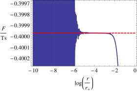
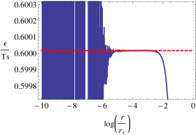
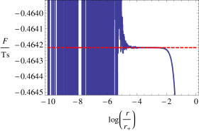
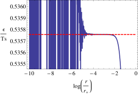
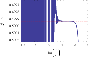
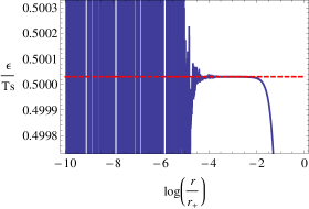
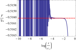
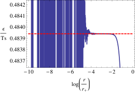
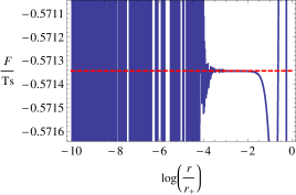
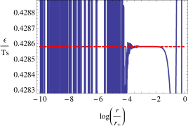
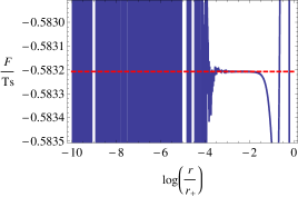
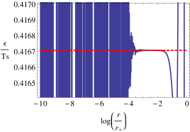
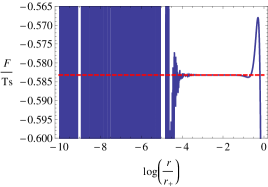
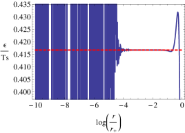
In the next section we shall numerically compute η(n,α~)𝜂𝑛~𝛼\eta(n,\tilde{\alpha}) function for n=4,5,,9𝑛459n=4,5,\ldots,9 for all values of α~~𝛼\tilde{\alpha} we consider. We will see that our results are consistent with (5.18) and (5.19) in all dimensions.

The lack of equality of the magnitudes of the free energy density and the energy density is also seen in (4.25)-(4.26) for Λ0similar-toΛ0\Lambda\sim 0, where \mathcal{F}\neq-\mathcal{E} when α~0~𝛼0\tilde{\alpha}\neq 0 even if ξ=0𝜉0\xi=0. This fact stands in contrast to the results for α~=0~𝛼0\tilde{\alpha}=0 Park:2012bv , in which =\mathcal{F}=-\mathcal{E} holds for Λ0similar-toΛ0\Lambda\sim 0 if β=0𝛽0\beta=0, where β𝛽\beta plays the same role as ξ𝜉\xi in this paper.

6.  Exploring Near the Quantum Critical Point

In holographic duality picture at zero temperature, we can imagine that the matter fields residing on the boundary of the spacetime become those of the conformal field theory, which is dual to the AdS spacetime in IR regimes, or the Lifshitz-like field theory (or quantum critical theory), which is dual to the Lifshitz spacetime in UV regimes. Our interests are to consider this configuration at finite temperature in the presence of the massive vector field and the Gauss-Bonnet terms in the gravity action, and to investigate the thermodynamic behaviour of the deformed GB-Lifshitz spacetime with a black hole, which from the duality perspective corresponds to the marginally relevant operators near the quantum critical point. To generate the marginally relevant modes, the momentum scale ΛΛ\Lambda is introduced into the asymptotic Lifshitz metric, and it is assumed that Λ0similar-toΛ0\Lambda\sim 0, which is much smaller than the background temperature T𝑇T (ΛzTmuch-less-thansuperscriptΛ𝑧𝑇\Lambda^{z}\ll T). Hence it slightly deforms the Lifshitz spacetime, recovering the pure Lifshitz spacetime for Λ=0Λ0\Lambda=0.

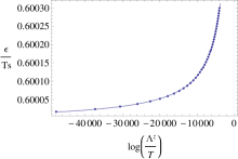
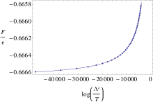
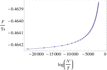
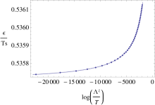
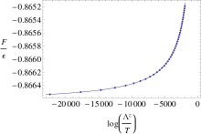
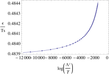
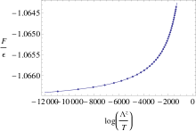
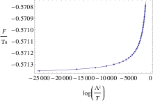
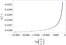
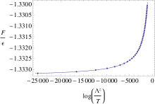
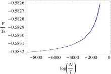
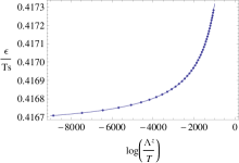
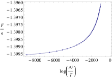
In this section, our aims are to show the implications of the Gauss-Bonnet terms for holographic renormalization flow and to observe the behaviour of physical quantities such as the free energy density /Ts𝑇𝑠\mathcal{F}/Ts and the energy density /Ts𝑇𝑠\mathcal{E}/Ts as functions of log(ΛzT)superscriptΛ𝑧𝑇\log(\frac{\Lambda^{z}}{T}).

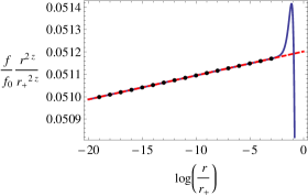
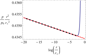
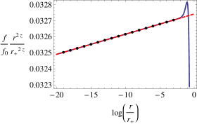
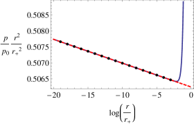
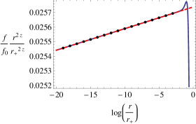
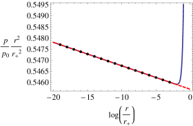
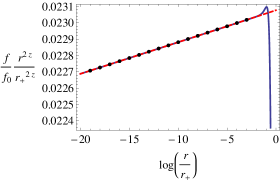
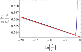
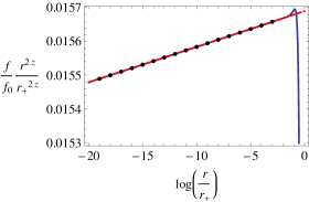
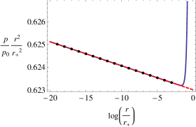
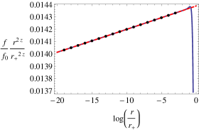
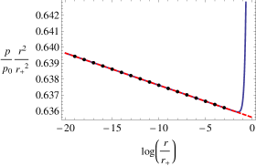
To do these, we first fix the undetermined parameters ΛΛ\Lambda, f0subscript𝑓0f_{0}, and p0subscript𝑝0p_{0} (in the numerical calculation we consider the quantities Λr+Λsubscript𝑟\Lambda r_{+}, ff0rzr+z𝑓subscript𝑓0superscript𝑟𝑧subscriptsuperscript𝑟𝑧\frac{f}{f_{0}}\frac{r^{z}}{r^{z}_{+}}, and pp0r2r+2𝑝subscript𝑝0superscript𝑟2subscriptsuperscript𝑟2\frac{p}{p_{0}}\frac{r^{2}}{r^{2}_{+}}). This is performed by numerically integrating the near horizon solution towards the boundary and reading off the matching values of ΛΛ\Lambda, f0subscript𝑓0f_{0}, and p0subscript𝑝0p_{0} in sections 6.1.1 and 6.1.2. Based on these values the thermodynamic functions \mathcal{F} and \mathcal{E} are numerically integrated from near horizon to the boundary, and their numerical values are found for each h0subscript0h_{0} in section 6.1.3. In section 6.2 we plot the data for \mathcal{F} and \mathcal{E} in a function of log(ΛzT)superscriptΛ𝑧𝑇\log(\frac{\Lambda^{z}}{T}).

6.1  Integrating towards the Lifshitz Boundary

As mentioned in section 5.1, we have scaling ambiguities in the metric due to the undetermined constants f0subscript𝑓0f_{0} and p0subscript𝑝0p_{0}. We here find values of ΛΛ\Lambda for each h0subscript0h_{0} by matching the numerical integration of near horizon solutions with the asymptotic solutions at the middle regions, and tune f0subscript𝑓0f_{0} and p0subscript𝑝0p_{0} with the matching value of ΛΛ\Lambda for the same h0subscript0h_{0} by using the same method. For the numerical calculation, we set up the arbitrary scale μ=r+1𝜇subscriptsuperscript𝑟1\mu=r^{-1}_{+} and use dimensionless quantities: rr+𝑟subscript𝑟\frac{r}{r_{+}}, Λr+Λsubscript𝑟\Lambda r_{+}, Ts𝑇𝑠\frac{\mathcal{F}}{Ts}, Ts𝑇𝑠\frac{\mathcal{E}}{Ts} and ΛzTsuperscriptΛ𝑧𝑇\frac{\Lambda^{z}}{T}.

Before performing the numerical work, we need to find the appropriate range of α~~𝛼\tilde{\alpha} and then choose specific values of α~~𝛼\tilde{\alpha}, as (5.1)-(5.3) describe a two-parameter family {h0,α~}subscript0~𝛼\{h_{0},\tilde{\alpha}\} of black hole solutions. The values of h0subscript0h_{0} will be computed for each α~~𝛼\tilde{\alpha} and will be discussed further in the following subsection.

Analyzing the asymptotic solutions (3.2)-(3.4) in section 2, recall that m2subscript𝑚2m_{2} yields the restriction α~14~𝛼14\tilde{\alpha}\leq\frac{1}{4}, where equality is not attained when z=𝑧z=\infty. We expect that |α~|<1~𝛼1|\tilde{\alpha}|<1 since the Gauss-Bonnet term associated with the coupling constant α~~𝛼\tilde{\alpha} via (2.10) is considered as a small correction to Einsteinian gravity. Then the range of α~~𝛼\tilde{\alpha} becomes

1<α~14,1~𝛼14-1<\tilde{\alpha}\leq\frac{1}{4}, (6.1)

and this corresponds to the range

n2z<3n5𝑛2𝑧3𝑛5\frac{n}{2}\leq z<3n-5 (6.2)

upon using z=n12(n2)α~𝑧𝑛12𝑛2~𝛼z=n-1-2(n-2)\tilde{\alpha} from (3.1). To observe the α~~𝛼\tilde{\alpha}-dependence for a broad range of values, we sparsely choose the values of α~~𝛼\tilde{\alpha}, which are the two positive values 1414\frac{1}{4}, 110110\frac{1}{10}, and three negative values 120120-\frac{1}{20} (bigger than 12(n2)12𝑛2-\frac{1}{2(n-2)}), 12(n2)12𝑛2-\frac{1}{2(n-2)}, 310310-\frac{3}{10} (smaller than 12(n2)12𝑛2-\frac{1}{2(n-2)}); we also consider α~=0~𝛼0\tilde{\alpha}=0 Park:2012bv for comparison. Table 1 lists the cases that we consider.

z𝑧z
α~=14~𝛼14\tilde{\alpha}=\frac{1}{4} α~=110~𝛼110\tilde{\alpha}=\frac{1}{10} α~=0~𝛼0\tilde{\alpha}=0 α~=120~𝛼120\tilde{\alpha}=-\frac{1}{20} α~=12(n2)~𝛼12𝑛2\tilde{\alpha}=-\frac{1}{2(n-2)} α~=310~𝛼310\tilde{\alpha}=-\frac{3}{10}
n=4𝑛4n=4 2 2.6 3 3.2 4 4.2
n=5𝑛5n=5 2.5 3.4 4 4.3 5 5.8
n=6𝑛6n=6 3 4.2 5 5.4 6 7.4
n=7𝑛7n=7 3.5 5 6 6.5 7 9
n=8𝑛8n=8 4 5.8 7 7.6 8 10.6
n=9𝑛9n=9 4.5 6.6 8 8.7 9 12.2
Table 1: values of z𝑧z according to n𝑛n and α~~𝛼\tilde{\alpha}

6.1.1 Matching ΛΛ\Lambda

In the asymptotic solutions (3.2)-(3.4), ΛΛ\Lambda is the only unfixed quantity. To fix ΛΛ\Lambda, we expand these solutions into the high energy regimes by introducing the arbitrary scale μ𝜇\mu and using the condition (3.10), which assumed that μΛmuch-greater-than𝜇Λ\mu\gg\Lambda. Then we set μ=r+𝜇subscript𝑟\mu=r_{+}, which means that our asymptotic solutions are described at the energy scale r+subscript𝑟r_{+}, and fit the asymptotic solutions towards the horizon.

Near the horizon the expanded black hole solutions (5.1)-(5.3) should be changed to the functions k𝑘k, q𝑞q, and y𝑦y by using the relations (3.10) so as to avoid the scale ambiguities of f0subscript𝑓0f_{0} and p0subscript𝑝0p_{0} for now. Then we numerically integrate the solutions towards the boundary by obeying the equations of the motion (2.24)-(2.26).

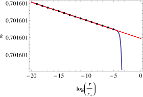
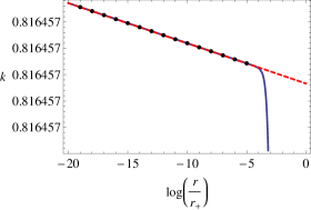
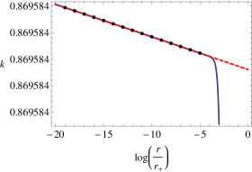
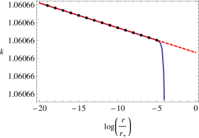
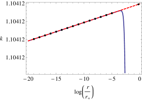
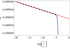
At the middle region, we match the fitting of the asymptotic solutions with the numerical integration for given h0subscript0h_{0} by controlling the value of logΛr+Λsubscript𝑟\log\Lambda r_{+} as shown in Fig. 2, which displays the function k𝑘k for n=4𝑛4n=4 and for each value of α~~𝛼\tilde{\alpha} in Table 1. The red dashed line is the fitted asymptotic solution, that is the one including logΛr+Λsubscript𝑟\log\Lambda r_{+}, and the blue solid line is the result of numerical integration of the horizon solution. In our numerical work, the integration is performed from log(r/r+)0.15similar-to𝑟subscript𝑟0.15\log(r/r_{+})\sim-0.15 to log(r/r+)104similar-to𝑟subscript𝑟superscript104\log(r/r_{+})\sim-10^{4}.

Note that in Fig. 2, the graph (f) shows the different behaviour from (a)-(e) by having a positive slope, which means that the k𝑘k function decreases as the boundary is approached. This positive-slope pattern is observed only for the k𝑘k function in the range α~<1/(2(n2))~𝛼12𝑛2\tilde{\alpha}<-1/(2(n-2)), which is equivalent to z>n𝑧𝑛z>n; for α~1/(2(n2))~𝛼12𝑛2\tilde{\alpha}\geq-1/(2(n-2)) or zn𝑧𝑛z\leq n, the slope of k𝑘k is negative, meaning it increases as the boundary is approached. The signs of the slopes of q𝑞q and y𝑦y versus log(r/r+)𝑟subscript𝑟\log(r/r_{+}) are negative for all values of α~~𝛼\tilde{\alpha}. Note that k𝑘k is defined via h=kf𝑘𝑓h=k\sqrt{f} from (2.22), where f𝑓f is the gttsubscript𝑔𝑡𝑡-g_{tt}-component of the metric and hh is the vector field potential. Hence k𝑘k only has information about the charge of the vector field and the Gauss-Bonnet coupling constant α~~𝛼\tilde{\alpha}. Fig. 2-(f) illustrates that when z>n𝑧𝑛z>n the weight for the charge of the vector field and α~~𝛼\tilde{\alpha} near the horizon become larger than at the boundary.
Refer to caption
(a) For α~=1/4~𝛼14\tilde{\alpha}=1/4 and n=4𝑛4n=4, h0=0.75120subscript00.75120h_{0}=0.75120 corresponds to log(Λr+)=23874.4Λsubscript𝑟23874.4\log(\Lambda r_{+})=-23874.4
Refer to caption
(b) For α~=1/10~𝛼110\tilde{\alpha}=1/10 and n=4𝑛4n=4, h0=1.26160subscript01.26160h_{0}=1.26160 corresponds to log(Λr+)=8611.8Λsubscript𝑟8611.8\log(\Lambda r_{+})=-8611.8
Refer to caption
(c) For α~=0~𝛼0\tilde{\alpha}=0 and n=4𝑛4n=4, h0=1.63430subscript01.63430h_{0}=1.63430 corresponds to log(Λr+)=5167.9Λsubscript𝑟5167.9\log(\Lambda r_{+})=-5167.9
Refer to caption
(d) For α~=1/20~𝛼120\tilde{\alpha}=-1/20 and n=4𝑛4n=4, h0=1.82980subscript01.82980h_{0}=1.82980 corresponds to log(Λr+)=3422Λsubscript𝑟3422\log(\Lambda r_{+})=-3422
Refer to caption
(e) For α~=1/4~𝛼14\tilde{\alpha}=-1/4 and n=4𝑛4n=4, h0=2.66868subscript02.66868h_{0}=2.66868 corresponds to log(Λr+)=4137.2Λsubscript𝑟4137.2\log(\Lambda r_{+})=-4137.2
Refer to caption
(f) For α~=3/10~𝛼310\tilde{\alpha}=-3/10 and n=4𝑛4n=4, h0=2.89170subscript02.89170h_{0}=2.89170 corresponds to log(Λr+)=2110.4Λsubscript𝑟2110.4\log(\Lambda r_{+})=-2110.4
Figure 2: Extracting log(Λr+)Λsubscript𝑟\log(\Lambda r_{+})

This process is performed by varying h0subscript0h_{0}. Beyond the maximum value of logΛr+Λsubscript𝑟\log\Lambda r_{+}, the numerical integration of the near horizon solution exponentially grows as the boundary is approached, and so does not match the asymptotic solution. This means that if the horizon flux ϕitalic-ϕ\phi in (5.8) is too large, which corresponds to high temperature, the deformation of the spacetime is not allowed any more and becomes the asymptotically pure Gauss-Bonnet-Lifshitz spacetime (having a black hole). Hence there exists a maximum value of h0subscript0h_{0}.

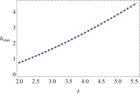
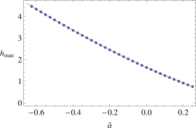
The maximum values of h0subscript0h_{0} are recorded in Table 2, and show linearly increasing dependence on the dimensionality of spacetime for the same α~~𝛼\tilde{\alpha}. For decreasing α~~𝛼\tilde{\alpha} the slope gets larger as shown in Fig. 3, where dots are the numerical data of the maximum value of h0subscript0h_{0} and the data obtained with the same value of α~~𝛼\tilde{\alpha} are connected with the line. For n=4𝑛4n=4, the dependence of α~~𝛼\tilde{\alpha} (or z𝑧z) on the maximum values of h0subscript0h_{0} is also found in Fig. 4, where the dots correspond to the maximum values of h0subscript0h_{0}, and the lines are the fitting functions obtained from the data. These are not linear; rather hmax0.633878+0.553198z+0.0680033z2similar-tosubscript𝑚𝑎𝑥0.6338780.553198𝑧0.0680033superscript𝑧2h_{max}\sim-0.633878+0.553198z+0.0680033z^{2} for Fig. 4(a) and hmax1.637753.84487α~+1.08805α~2similar-tosubscript𝑚𝑎𝑥1.637753.84487~𝛼1.08805superscript~𝛼2h_{max}\sim 1.63775-3.84487\tilde{\alpha}+1.08805\tilde{\alpha}^{2} for Fig. 4(b). These results indicate that h0subscript0h_{0} obviously depends on α~~𝛼\tilde{\alpha}.

A minimum value of the flux also exists; its value becomes zero at the horizon. In this case, the influence of the massive vector field vanishes, and so the spacetime is described completely by an asymptotically Gauss-Bonnet AdS black hole.

Very small values of h0subscript0h_{0} correspond to the zero temperature limit Λz/TsuperscriptΛ𝑧𝑇\Lambda^{z}/T\rightarrow\infty; in this limit the AdS spacetime emerges in the IR regime. Hence for fixed Λ0similar-toΛ0\Lambda\sim 0, the slightly deformed UV Lifshitz spacetime and IR AdS spacetime with Gauss-Bonnet corrections emerge instead. Thus we might expect holographic renormalization group flow at zero temperature similar to the α~=0~𝛼0\tilde{\alpha}=0 case Braviner:2011kz ,Kachru:2008yh . The presence and nature of the renormalization flow interpolating both spacetimes for α~0~𝛼0\tilde{\alpha}\neq 0 has not yet been studied yet; it remains for future work.
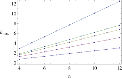
Refer to caption
Figure 3: Dots are the maximum value of h0subscript0h_{0} for given n𝑛n and α~~𝛼\tilde{\alpha}, and dots sharing the same α~~𝛼\tilde{\alpha} are connected with the same color of line to distinguish them. From the bottom, each different color of line respectively indicates α~=14,110,0,120~𝛼141100120\tilde{\alpha}=\frac{1}{4},\frac{1}{10},0,-\frac{1}{20}, and 310310-\frac{3}{10}.
hmaxsubscript𝑚𝑎𝑥h_{max}
α~=14~𝛼14\tilde{\alpha}=\frac{1}{4} α~=110~𝛼110\tilde{\alpha}=\frac{1}{10} α~=0~𝛼0\tilde{\alpha}=0 α~=120~𝛼120\tilde{\alpha}=-\frac{1}{20} α~=12(n2)~𝛼12𝑛2\tilde{\alpha}=-\frac{1}{2(n-2)} α~=310~𝛼310\tilde{\alpha}=-\frac{3}{10}
n=4𝑛4n=4 0.7512 1.2616 1.6343 1.8298 2.6687 2.8917
n=5𝑛5n=5 1.0416 1.7528 2.2822 2.5622 3.2519 4.0981
n=6𝑛6n=6 1.3288 2.2394 2.9255 3.2900 3.8614 5.3005
n=7𝑛7n=7 1.6147 2.7239 3.5668 4.0158 4.4818 6.5012
n=8𝑛8n=8 1.8998 3.2073 4.2070 4.7406 5.1079 7.7011
n=9𝑛9n=9 2.1844 3.6900 4.8465 5.4647 5.7372 8.9004
n=10𝑛10n=10 2.4688 4.1723 5.4856 6.1884 6.3686 10.0992
n=11𝑛11n=11 2.7530 4.6543 6.1244 6.9118 7.0013 11.2977
n=12𝑛12n=12 3.0371 5.1361 6.7629 7.6346 7.6349 12.4958
\vdots \vdots \vdots \vdots \vdots \vdots \vdots
Table 2: The maximum values of h0subscript0h_{0} for each values of n𝑛n and α~~𝛼\tilde{\alpha}
Refer to caption
(a) The maximum value of h0subscript0h_{0} on z𝑧z
Refer to caption
(b) The maximum value of h0subscript0h_{0} on α~~𝛼\tilde{\alpha}
Figure 4: Dependence of z𝑧z or α~~𝛼\tilde{\alpha} on hmaxsubscript𝑚𝑎𝑥h_{max} when n=4𝑛4n=4.

6.1.2 Matching f0subscript𝑓0f_{0} and p0subscript𝑝0p_{0}

We have other variables left to be determined, which are f0subscript𝑓0f_{0} and p0subscript𝑝0p_{0} in (5.1)-(5.3). Since ΛΛ\Lambda is fixed, we tune f0subscript𝑓0f_{0} and p0subscript𝑝0p_{0} based on the value of ΛΛ\Lambda for each set {h0,α~}subscript0~𝛼\{h_{0},\tilde{\alpha}\} by using the same method applied for ΛΛ\Lambda.

We bring the asymptotic solutions (3)-(3.12) expanded in the high energy regime in terms of μ𝜇\mu, where μ=r+1𝜇subscriptsuperscript𝑟1\mu=r^{-1}_{+}, and fit the solutions with the determined value of ΛΛ\Lambda (given {h0,α~}subscript0~𝛼\{h_{0},\tilde{\alpha}\}) to the horizon. Near the horizon, we numerically integrate the the equations of motion (2.19)-(2.21) towards the boundary using (5.1)-(5.3) as initial conditions. At the middle region, we adjust f0r+2zsubscript𝑓0subscriptsuperscript𝑟2𝑧f_{0}r^{2z}_{+} or p0r+2subscript𝑝0subscriptsuperscript𝑟2p_{0}r^{2}_{+} and read off the values for which both solutions agree. This process for f𝑓f and p𝑝p functions is depicted in Figures 5 and 6 for α~=1/4,1/10,0,1/20,1/4,3/10~𝛼14110012014310\tilde{\alpha}=1/4,1/10,0,-1/20,-1/4,-3/10 for n=4𝑛4n=4. The red dashed line is the fit of the boundary solution and the blue solid line is the numerical result of the near horizon solution. For n=5,6,7,8,9𝑛56789n=5,6,7,8,9 higher-dimensional cases we find similar patterns for the same values of α~~𝛼\tilde{\alpha}.

Refer to caption
Refer to caption
(a) For α~=1/4~𝛼14\tilde{\alpha}=1/4 (z=2𝑧2z=2) and h0=0.75120subscript00.75120h_{0}=0.75120, which corresponds to log(Λr+)=23874.4Λsubscript𝑟23874.4\log(\Lambda r_{+})=-23874.4, the red dashed line is matched to the blue solid line at f0r+2z=19.66subscript𝑓0subscriptsuperscript𝑟2𝑧19.66f_{0}r^{2z}_{+}=19.66 (left) and p0r+2=2.2942subscript𝑝0subscriptsuperscript𝑟22.2942p_{0}r^{2}_{+}=2.2942 (right). The dots correspond to the values for finding the matching condition.
Refer to caption
Refer to caption
(b) For α~=1/10~𝛼110\tilde{\alpha}=1/10 (z=2.6) and h0=1.26160subscript01.26160h_{0}=1.26160, which corresponds to log(Λr+)=8611.8Λsubscript𝑟8611.8\log(\Lambda r_{+})=-8611.8, the red dashed line is matched to the blue solid line at f0r+2z=30.66subscript𝑓0subscriptsuperscript𝑟2𝑧30.66f_{0}r^{2z}_{+}=30.66 (left) and p0r+2=1.9725subscript𝑝0subscriptsuperscript𝑟21.9725p_{0}r^{2}_{+}=1.9725 (right). The dots correspond to the values for finding the matching condition.
Refer to caption
Refer to caption
(c) For α~=0~𝛼0\tilde{\alpha}=0 (z=3) and h0=1.63430subscript01.63430h_{0}=1.63430, which corresponds to log(Λr+)=5167.9Λsubscript𝑟5167.9\log(\Lambda r_{+})=5167.9, the red dashed line is matched to the blue solid line at f0r+2z=39.00subscript𝑓0subscriptsuperscript𝑟2𝑧39.00f_{0}r^{2z}_{+}=39.00 (left) and p0r+2=1.8303subscript𝑝0subscriptsuperscript𝑟21.8303p_{0}r^{2}_{+}=1.8303 (right). The dots correspond to the values for finding the matching condition.
Figure 5: Extracting f0subscript𝑓0f_{0} and p0subscript𝑝0p_{0} for positive and zero α~~𝛼\tilde{\alpha} for n=4𝑛4n=4
Refer to caption
Refer to caption
(a) For α~=1/20~𝛼120\tilde{\alpha}=-1/20 (z=3.2𝑧3.2z=3.2) and h0=1.82980subscript01.82980h_{0}=1.82980, which corresponds to log(Λr+)=3422Λsubscript𝑟3422\log(\Lambda r_{+})=-3422, the red dashed line is matched to the blue solid line at f0r+2z=43.53subscript𝑓0subscriptsuperscript𝑟2𝑧43.53f_{0}r^{2z}_{+}=43.53 (left) and p0r+2=1.7727subscript𝑝0subscriptsuperscript𝑟21.7727p_{0}r^{2}_{+}=1.7727 (right). The dots correspond to the values for finding the matching condition.
Refer to caption
Refer to caption
(b) For α~=1/4~𝛼14\tilde{\alpha}=-1/4 (z=4𝑧4z=4) and h0=2.66868subscript02.66868h_{0}=2.66868, which corresponds to log(Λr+)=4137.2Λsubscript𝑟4137.2\log(\Lambda r_{+})=-4137.2, the red dashed line is matched to the blue solid line at f0r+2z=63.88subscript𝑓0subscriptsuperscript𝑟2𝑧63.88f_{0}r^{2z}_{+}=63.88 (left) and p0r+2=1.6042subscript𝑝0subscriptsuperscript𝑟21.6042p_{0}r^{2}_{+}=1.6042 (right). The dots correspond to the values for finding the matching condition.
Refer to caption
Refer to caption
(c) For α~=3/10~𝛼310\tilde{\alpha}=-3/10 (z=4.2𝑧4.2z=4.2) and h0=2.89170subscript02.89170h_{0}=2.89170, which corresponds to log(Λr+)=2110.4Λsubscript𝑟2110.4\log(\Lambda r_{+})=-2110.4, the red dashed line is matched to the blue solid line at f0r+2z=69.76subscript𝑓0subscriptsuperscript𝑟2𝑧69.76f_{0}r^{2z}_{+}=69.76 (left) and p0r+2=1.5719subscript𝑝0subscriptsuperscript𝑟21.5719p_{0}r^{2}_{+}=1.5719 (right). The dots correspond to the values for finding the matching condition.
Figure 6: Extracting f0subscript𝑓0f_{0} and p0subscript𝑝0p_{0} for negative α~~𝛼\tilde{\alpha} for n=4𝑛4n=4

Since we have now fixed ΛΛ\Lambda, f0subscript𝑓0f_{0}, and p0subscript𝑝0p_{0}, the thermodynamic quantities calculated in (5.8) can be determined. The temperature is given by

log(ΛzT)=zlog(Λr+)+log(2π)12log(f0r+2z)superscriptΛ𝑧𝑇𝑧Λsubscript𝑟2𝜋12subscript𝑓0subscriptsuperscript𝑟2𝑧\log\bigg{(}\frac{\Lambda^{z}}{T}\bigg{)}=z\log(\Lambda r_{+})+\log(2\pi)-\frac{1}{2}\log(f_{0}r^{2z}_{+}) (6.3)

which is computed from the known values of ΛΛ\Lambda and f0subscript𝑓0f_{0}. In next sections, we collect all data on the free energy density /Ts𝑇𝑠\mathcal{F}/Ts and the energy density /Ts𝑇𝑠\mathcal{E}/Ts for given {h0,α~}subscript0~𝛼\{h_{0},\tilde{\alpha}\}, where the specific value of h0subscript0h_{0} corresponds to each set of values {Λ,f0,p0}Λsubscript𝑓0subscript𝑝0\{\Lambda,f_{0},p_{0}\}, and fit their results to a function of logΛz/TsuperscriptΛ𝑧𝑇\log\Lambda^{z}/T. We consider the dimensionless quantities /Ts𝑇𝑠\mathcal{F}/Ts and /Ts𝑇𝑠\mathcal{E}/Ts. For the entropy density s𝑠s from (5.8), we consider the dimensionless quantity s/Tn1z𝑠superscript𝑇𝑛1𝑧s/T^{\frac{n-1}{z}} as a function of log(Λz/T)superscriptΛ𝑧𝑇\log(\Lambda^{z}/T), plotted in Fig. 13.

6.1.3 Free Energy Density and Energy Density

The dimensionless quantities /Ts𝑇𝑠\mathcal{F}/Ts and /Ts𝑇𝑠\mathcal{E}/Ts, respectively the free energy density (4.7) and the energy density (4.19), are numerically integrated from the horizon towards the boundary for given {h0,α~}subscript0~𝛼\{h_{0},\tilde{\alpha}\}. The results are depicted in Figures 7 and 8, where the blue line is the numerical result and the red dashed line is read off from the stable value in the flat region. As shown in Figures 7 and 8, /Ts𝑇𝑠\mathcal{F}/Ts and /Ts𝑇𝑠\mathcal{E}/Ts yield constant values over some finite range of log(r/r+)𝑟subscript𝑟\log(r/r_{+}), but oscillate infinitely upon approaching the boundary. The reason for these diverging and oscillating behaviours can be found in the holographic renormalization process in section 3. Recall that the free energy density and the energy density diverge as r0𝑟0r\rightarrow 0, and so the counterterms (4.22)-(4.24) were constructed to render them finite. As mentioned, C0subscript𝐶0C_{0} and C1subscript𝐶1C_{1} expand to infinite series in log(Λr+)Λsubscript𝑟\log(\Lambda r_{+}); however only terms up to 1/log4(Λr)1superscript4Λ𝑟1/\log^{4}(\Lambda r) (15 terms for each of C0subscript𝐶0C_{0} and C1subscript𝐶1C_{1}) are computed due to limitations of the analytic calculation. This finite number of terms is employed in the numerical calculation of /Ts𝑇𝑠\mathcal{F}/Ts and /Ts𝑇𝑠\mathcal{E}/Ts. On the other hand, the numerical work includes higher orders (i.e. higher than 1/log4Λr1superscript4Λ𝑟1/\log^{4}\Lambda r), and so the diverging properties are not totally eliminated by our analytic solutions using counterterms.

In Figures 8 (b) and (c), which corresponds to cases of z=4𝑧4z=4 and z=4.2𝑧4.2z=4.2 respectively, unstable behaviours are observed near the horizon. To see the whole pattern the scales are zoomed out in Figure 8 (d). This pattern of having a sharp peak near the horizon commonly appears for the range zngreater-than-or-equivalent-to𝑧𝑛z\gtrsim n for any n𝑛n and h0subscript0h_{0}. The unstable behaviour of /Ts𝑇𝑠\mathcal{F}/Ts and /Ts𝑇𝑠\mathcal{E}/Ts for zngreater-than-or-equivalent-to𝑧𝑛z\gtrsim n can be understood via the same rationale for the different pattern of the k𝑘k-function for z>n𝑧𝑛z>n. That is, as z𝑧z gets bigger and approaches znsimilar-to𝑧𝑛z\sim n due to the decreasing value of α~~𝛼\tilde{\alpha}, the effect of both the charge of the vector field and α~~𝛼\tilde{\alpha} gets bigger near the horizon than at the boundary, causing unstable behaviour in both /Ts𝑇𝑠\mathcal{F}/Ts and /Ts𝑇𝑠\mathcal{E}/Ts.

Refer to caption
Refer to caption
(a) For α~=1/4~𝛼14\tilde{\alpha}=1/4 (z=2𝑧2z=2) and h0=0.75120subscript00.75120h_{0}=0.75120, which corresponds to log(Λr+)=23874.4Λsubscript𝑟23874.4\log(\Lambda r_{+})=-23874.4. Blue line is the numerical results of the free energy density over Ts𝑇𝑠Ts (left) and the energy density over Ts𝑇𝑠Ts (right), and red dashed line is reading-off the constant value in the intermediate regime.
Refer to caption
Refer to caption
(b) For α~=1/10~𝛼110\tilde{\alpha}=1/10 (z=2.6𝑧2.6z=2.6) and h0=1.26156subscript01.26156h_{0}=1.26156, which corresponds to log(Λr+)=5648.3Λsubscript𝑟5648.3\log(\Lambda r_{+})=-5648.3. Blue line is the numerical results of the free energy density over Ts𝑇𝑠Ts (left) and the energy density over Ts𝑇𝑠Ts (right), and red dashed line is reading-off the constant value in the intermediate regime.
Refer to caption
Refer to caption
(c) For α~=0~𝛼0\tilde{\alpha}=0 (z=3) and h0=1.63430subscript01.63430h_{0}=1.63430, which corresponds to log(Λr+)=5167.9Λsubscript𝑟5167.9\log(\Lambda r_{+})=5167.9. Blue line is the numerical results of the free energy density over Ts𝑇𝑠Ts (left) and the energy density over Ts𝑇𝑠Ts (right), and red dashed line is reading-off the constant value in the intermediate regime.
Figure 7: /Ts𝑇𝑠{\mathcal{F}}/Ts and /Ts𝑇𝑠{\mathcal{E}}/Ts versus log(rr+)𝑟subscript𝑟\log(\frac{r}{r_{+}}) for positive and zero α~~𝛼\tilde{\alpha} for n=4𝑛4n=4
Refer to caption
Refer to caption
(a) For α~=1/10~𝛼110\tilde{\alpha}=-1/10 (z=3.2𝑧3.2z=3.2) and h0=1.82976subscript01.82976h_{0}=1.82976, which corresponds to log(Λr+)=2523.1Λsubscript𝑟2523.1\log(\Lambda r_{+})=-2523.1.
Refer to caption
Refer to caption
(b) For α~=1/4~𝛼14\tilde{\alpha}=-1/4 (z=4𝑧4z=4) and h0=2.66868subscript02.66868h_{0}=2.66868, which corresponds to log(Λr+)=4137.2Λsubscript𝑟4137.2\log(\Lambda r_{+})=-4137.2.
Refer to caption
Refer to caption
(c) For α~=3/10~𝛼310\tilde{\alpha}=-3/10 (z=4.2𝑧4.2z=4.2) and h0=2.89170subscript02.89170h_{0}=2.89170, which corresponds to log(Λr+)=2110.4Λsubscript𝑟2110.4\log(\Lambda r_{+})=-2110.4.
Refer to caption
Refer to caption
(d) enlarged graphs of the above (c)
Figure 8: /Ts𝑇𝑠{\mathcal{F}}/Ts and /Ts𝑇𝑠{\mathcal{E}}/Ts versus log(rr+)𝑟subscript𝑟\log(\frac{r}{r_{+}}) for negative α~~𝛼\tilde{\alpha} for n=4𝑛4n=4

6.2  Behaviours of \mathcal{F} and \mathcal{E} near Quantum Critical Regimes

Collecting data for each of the values of {h0,α~}subscript0~𝛼\{h_{0},\tilde{\alpha}\}, we plot /Ts𝑇𝑠\mathcal{F}/Ts and /Ts𝑇𝑠\mathcal{E}/Ts as functions of logΛz/TsuperscriptΛ𝑧𝑇\log\Lambda^{z}/T and find their fitting functions. These results are displayed in Figures 10 and 11, for which n=4𝑛4n=4; the dots are the numerical results and the solid line is the fitting function found. The fitting functions for each n𝑛n are recorded in Tables 3, 5, 6, 7, 8, and 9. We subsequently check that our numerical results for /Ts𝑇𝑠\mathcal{F}/Ts and /Ts𝑇𝑠\mathcal{E}/Ts with the marginally relevant modes agree with the integrated first law of thermodynamics in (5.15) with an error of less than 104superscript10410^{-4} as shown in Fig. 12.

It is straightforward to show using the data in the rightmost columns of tables 3, 5, 6, 7, 8, and 9, that the values of 0/0=η(n,α~)subscript0subscript0𝜂𝑛~𝛼\mathcal{F}_{0}/\mathcal{E}_{0}=-\eta(n,\tilde{\alpha}) are consistent with the expression (5.18). We illustrate the n=4𝑛4n=4 case in Fig. 9, where the red dots are the numerical data and the solid line is the expression for η(4,α~)𝜂4~𝛼\eta(4,\tilde{\alpha}) given in (5.18). We recover the values of 0/Tssubscript0𝑇𝑠\mathcal{F}_{0}/Ts and 0/Tssubscript0𝑇𝑠\mathcal{E}_{0}/Ts in (5.19) in the absence of the marginally relevant mode (Λ=0Λ0\Lambda=0) at finite temperature.

(n=4𝑛4n=4) Ts𝑇𝑠\frac{{\mathcal{F}}}{Ts} Ts𝑇𝑠\frac{\mathcal{E}}{Ts} \frac{\mathcal{F}}{\mathcal{E}}
α~=1/4~𝛼14\tilde{\alpha}=1/4 or z=2𝑧2z=2 0.401.21logΛz/T+0.401.21superscriptΛ𝑧𝑇\;-0.40-\frac{1.21}{\log\Lambda^{z}/T}+\cdots  0.601.21logΛz/T+0.601.21superscriptΛ𝑧𝑇\;0.60-\frac{1.21}{\log\Lambda^{z}/T}+\cdots 0.673.37logΛz/T+0.673.37superscriptΛ𝑧𝑇\;-0.67-\frac{3.37}{\log\Lambda^{z}/T}+\cdots
α~=1/10~𝛼110\tilde{\alpha}=1/10 or z=2.6𝑧2.6z=2.6 0.460.83logΛz/T+0.460.83superscriptΛ𝑧𝑇\;-0.46-\frac{0.83}{\log\Lambda^{z}/T}+\cdots  0.540.83logΛz/T+0.540.83superscriptΛ𝑧𝑇\;0.54-\frac{0.83}{\log\Lambda^{z}/T}+\cdots 0.872.89logΛz/T+0.872.89superscriptΛ𝑧𝑇\;-0.87-\frac{2.89}{\log\Lambda^{z}/T}+\cdots
α~=0~𝛼0\tilde{\alpha}=0 or z=3𝑧3z=3 0.500.76logΛz/T+0.500.76superscriptΛ𝑧𝑇\;-0.50-\frac{0.76}{\log\Lambda^{z}/T}+\cdots  0.500.76logΛz/T+0.500.76superscriptΛ𝑧𝑇\;0.50-\frac{0.76}{\log\Lambda^{z}/T}+\cdots 1.03.00logΛz/T+1.03.00superscriptΛ𝑧𝑇\;-1.0-\frac{3.00}{\log\Lambda^{z}/T}+\cdots
α~=1/20~𝛼120\tilde{\alpha}=-1/20 or z=3.2𝑧3.2z=3.2 0.520.73logΛz/T+0.520.73superscriptΛ𝑧𝑇\;-0.52-\frac{0.73}{\log\Lambda^{z}/T}+\cdots  0.480.74logΛz/T+0.480.74superscriptΛ𝑧𝑇\;0.48-\frac{0.74}{\log\Lambda^{z}/T}+\cdots 1.13.13logΛz/T+1.13.13superscriptΛ𝑧𝑇\;-1.1-\frac{3.13}{\log\Lambda^{z}/T}+\cdots
α~=1/4~𝛼14\tilde{\alpha}=-1/4 or z=4𝑧4z=4 0.570.69logΛz/T+0.570.69superscriptΛ𝑧𝑇\;-0.57-\frac{0.69}{\log\Lambda^{z}/T}+\cdots  0.430.69logΛz/T+0.430.69superscriptΛ𝑧𝑇\;0.43-\frac{0.69}{\log\Lambda^{z}/T}+\cdots 1.33.76logΛz/T+1.33.76superscriptΛ𝑧𝑇\;-1.3-\frac{3.76}{\log\Lambda^{z}/T}+\cdots
α~=3/10~𝛼310\tilde{\alpha}=-3/10 or z=4.2𝑧4.2z=4.2 0.580.69logΛz/T+0.580.69superscriptΛ𝑧𝑇\;-0.58-\frac{0.69}{\log\Lambda^{z}/T}+\cdots  0.420.69logΛz/T+0.420.69superscriptΛ𝑧𝑇\;0.42-\frac{0.69}{\log\Lambda^{z}/T}+\cdots 1.43.95logΛz/T+1.43.95superscriptΛ𝑧𝑇\;-1.4-\frac{3.95}{\log\Lambda^{z}/T}+\cdots
\vdots \vdots \vdots \vdots
Table 3: fitting functions for Ts𝑇𝑠\frac{{\mathcal{F}}}{Ts}, Ts𝑇𝑠\frac{\mathcal{E}}{Ts}, and \frac{\mathcal{F}}{\mathcal{E}}

We also observed how /Ts𝑇𝑠\mathcal{F}/Ts and /Ts𝑇𝑠\mathcal{E}/Ts behave with the marginally relevant modes according to different values of n𝑛n and α~~𝛼\tilde{\alpha} when Λz/T0superscriptΛ𝑧𝑇0\Lambda^{z}/T\rightarrow 0. When Λ0Λ0\Lambda\neq 0 the marginally relevant modes (generated by small values of ΛΛ\Lambda) contribute at sub-leading order to /Ts𝑇𝑠\mathcal{F}/Ts and /Ts𝑇𝑠\mathcal{E}/Ts as functions of logΛz/TsuperscriptΛ𝑧𝑇\log\Lambda^{z}/T, where Λz/T0superscriptΛ𝑧𝑇0\Lambda^{z}/T\rightarrow 0. From Figures 10, 11 and Tables 3, 5, 6, 7, 8, and 9, we see that for the same dimension n𝑛n, as z𝑧z increases (or α~~𝛼\tilde{\alpha} decreases), this sub-leading contribution decreases. Furthermore, for the same value of α~~𝛼\tilde{\alpha}, as z𝑧z increases (or n𝑛n increases), this sub-leading contribution also decreases. That is, when z𝑧z increases due to either decreasing α~~𝛼\tilde{\alpha} or increasing n𝑛n by z=n12(n2)α~𝑧𝑛12𝑛2~𝛼z=n-1-2(n-2)\tilde{\alpha}, this sub-leading contribution decreases.
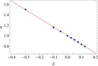
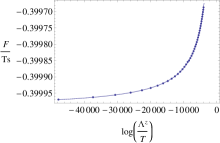
Refer to caption
Figure 9: For n=4𝑛4n=4, red dots are the numerical data and blue solid line is the fitting of the η𝜂\eta function
Refer to caption
Refer to caption
Refer to caption
(a) For α=14𝛼14\alpha=\frac{1}{4} (or z=2𝑧2z=2). Dots are numerical results running h0subscript0h_{0} from 0.751200.751200.75120 to 0.750380.750380.75038, which corresponds to logΛz/TsuperscriptΛ𝑧𝑇\log\Lambda^{z}/T from 47748.547748.5-47748.5 to 3945.483945.48-3945.48. Solid line is the fitting function denoted in Table 3.
Refer to caption
Refer to caption
Refer to caption
(b) For α=110𝛼110\alpha=\frac{1}{10} (or z=2.6𝑧2.6z=2.6). Dots are numerical results running h0subscript0h_{0} from 1.261601.261601.26160 to 1.260781.260781.26078, which corresponds to logΛz/TsuperscriptΛ𝑧𝑇\log\Lambda^{z}/T from 22390.622390.6-22390.6 to 1960.291960.29-1960.29. Solid line is the fitting function denoted in Table 3.
Refer to caption
Refer to caption
Refer to caption
(c) For α=0𝛼0\alpha=0 (or z=3𝑧3z=3). Dots are numerical results running h0subscript0h_{0} from 1.634301.634301.63430 to 1.633481.633481.63348, which corresponds to logΛz/TsuperscriptΛ𝑧𝑇\log\Lambda^{z}/T from 15503.715503.7-15503.7 to 15522.5115522.51-15522.51. Solid line is the fitting function denoted in Table 3.
Figure 10: Plots of /Ts𝑇𝑠{\mathcal{F}}/Ts , /Ts𝑇𝑠{\mathcal{E}}/Ts and /{\mathcal{F}}/{\mathcal{E}} versus log(Λz/T)superscriptΛ𝑧𝑇\log(\Lambda^{z}/T) for positive and zero α~~𝛼\tilde{\alpha} for n=4𝑛4n=4
Refer to caption
Refer to caption
Refer to caption
(a) For α=120𝛼120\alpha=-\frac{1}{20} (or z=3.2𝑧3.2z=3.2). Dots are numerical results running h0subscript0h_{0} from 1.829801.829801.82980 to 1.828981.828981.82898, which corresponds to logΛz/TsuperscriptΛ𝑧𝑇\log\Lambda^{z}/T from 10950.410950.4-10950.4 to 1354.621354.62-1354.62. Solid line is the fitting function denoted in Table 3.
Refer to caption
Refer to caption
Refer to caption
(b) For α~=14~𝛼14\tilde{\alpha}=-\frac{1}{4} (or z=4𝑧4z=4). Dots are numerical results running h0subscript0h_{0} from 2.668702.668702.66870 to 2.667882.667882.66788, which corresponds to logΛz/TsuperscriptΛ𝑧𝑇\log\Lambda^{z}/T from 24978.224978.2-24978.2 to 1147.851147.85-1147.85. Solid line is the fitting function denoted in Table 3.
Refer to caption
Refer to caption
Refer to caption
(c) For α~=310~𝛼310\tilde{\alpha}=-\frac{3}{10} (or z=4.2𝑧4.2z=4.2). Dots are numerical results running h0subscript0h_{0} from 2.891702.891702.89170 to 2.890882.890882.89088, which corresponds to logΛz/TsuperscriptΛ𝑧𝑇\log\Lambda^{z}/T from 8863.968863.96-8863.96 to 1051.131051.13-1051.13. Solid line is the fitting function denoted in Table 3.
Figure 11: Plots of /Ts𝑇𝑠{\mathcal{F}}/Ts , /Ts𝑇𝑠{\mathcal{E}}/Ts and /{\mathcal{F}}/{\mathcal{E}} versus log(Λz/T)superscriptΛ𝑧𝑇\log(\Lambda^{z}/T) for negative α~~𝛼\tilde{\alpha} for n=4𝑛4n=4.
Refer to caption
(a) For α~=14~𝛼14\tilde{\alpha}=\frac{1}{4} (orz=2𝑜𝑟𝑧2orz=2) and h0subscript0h_{0} runs from 0.751200.751200.75120 to 0.750380.750380.75038.
Refer to caption
(b) For α~=110~𝛼110\tilde{\alpha}=\frac{1}{10} (or z=2.6𝑧2.6z=2.6) and h0subscript0h_{0} from 1.261601.261601.26160 to 1.260781.260781.26078.
Refer to caption
(c) For α~=0~𝛼0\tilde{\alpha}=0 (or z=3𝑧3z=3) and h0subscript0h_{0} runs from 1.634301.634301.63430 to 1.633481.633481.63348
Refer to caption
(d) For α~=120~𝛼120\tilde{\alpha}=-\frac{1}{20} (or z=3.2𝑧3.2z=3.2) and h0subscript0h_{0} runs from 1.829801.829801.82980 to 1.828981.828981.82898
Refer to caption
(e) For α~=14~𝛼14\tilde{\alpha}=-\frac{1}{4} (or z=4𝑧4z=4) and h0subscript0h_{0} runs from 2.668702.668702.66870 to 2.667882.667882.66788
Refer to caption
(f) For α~=310~𝛼310\tilde{\alpha}=-\frac{3}{10} (or z=4.2𝑧4.2z=4.2). h0subscript0h_{0} runs from 2.891702.891702.89170 to 2.890882.890882.89088
Figure 12: Plots of errors from /Ts+/Ts1𝑇𝑠𝑇𝑠1-\mathcal{F}/Ts+\mathcal{E}/Ts-1

7.  Summary and Discussion

Our main purpose has been to understand how the Gauss-Bonnet coupling constant α~~𝛼\tilde{\alpha}, defined in (2.10), plays a role in the deformation of Lifshitz holography in (n+1𝑛1n+1) dimensions.

First recall where α~~𝛼\tilde{\alpha} makes a contribution. In the Lifshitz spacetime without the Gauss-Bonnet term (α~=0~𝛼0\tilde{\alpha}=0), the anisotropy of the spacetime is governed by the massive vector field. This vector field allows a (non-trivial) marginally relevant mode only at z=(n1)𝑧𝑛1z=(n-1) Park:2012bv . When the Gauss-Bonnet term is included in the Lifshitz gravity action, the (non-trivial) marginally relevant mode is now restricted by z=n12(n2)α~𝑧𝑛12𝑛2~𝛼z=n-1-2(n-2)\tilde{\alpha}. In other words z𝑧z is determined not only by the massive vector field but also by the value of α~~𝛼\tilde{\alpha}. Considering the marginal mode in the pure Lifshitz case (i.e. Λ=0Λ0\Lambda=0) for the metric (2.15), α~~𝛼\tilde{\alpha} contributes to the function f=1r2z𝑓1superscript𝑟2𝑧f=\frac{1}{r^{2z}} in the metric via z𝑧z and also modifies the charge of the massive vector field by q2=z1z(12α~)superscript𝑞2𝑧1𝑧12~𝛼q^{2}=\frac{z-1}{z}(1-2\tilde{\alpha}). However, in the deformed Lifshitz spacetime (i.e. considering marginally relevant modes generated by Λ0similar-toΛ0\Lambda\sim 0), α~~𝛼\tilde{\alpha} modifies both f𝑓f and p𝑝p in the metric with ΛΛ\Lambda and involves the massive vector field, as shown in (3.2)-(3.4) or (3.7)-(3.8).

We found the asymptotic solutions in (3.2)-(3.4), and obtained the free energy density in (4.7) and the energy density in (4.19) by holographic renormalization. We next derived the near-horizon expansion of the black hole solution in (5.1)-(5.3), characterized by two parameters h0subscript0h_{0} and α~~𝛼\tilde{\alpha}, and calculated thermodynamic quantities such as temperature T𝑇T and entropy density s𝑠s in (5.8). As our metric solutions contain undetermined parameters ΛΛ\Lambda in the asymptotic solution and f0subscript𝑓0f_{0} and p0subscript𝑝0p_{0} in the near horizon solution, we numerically integrate the horizon solution towards to boundary and match it with the asymptotic solution plotted towards the horizon by controlling ΛΛ\Lambda, f0subscript𝑓0f_{0}, and p0subscript𝑝0p_{0} for given {h0,α~}subscript0~𝛼\{h_{0},\tilde{\alpha}\}. After fixing those parameters, we numerically explored physical quantities such as the free energy density and the energy density.

Numerically we found that there exists a maximum value of h0subscript0h_{0}, which corresponds to high temperature Λz/T0superscriptΛ𝑧𝑇0\Lambda^{z}/T\rightarrow 0. The smaller the value of α~~𝛼\tilde{\alpha} (or larger z𝑧z) , the larger the maximum value of h0subscript0h_{0}. This explicitly demonstrates that α~~𝛼\tilde{\alpha} modifies h0subscript0h_{0} or the horizon flux of the vector field via h0subscript0h_{0}. The dependence of the maximum value of h0subscript0h_{0} both on α~~𝛼\tilde{\alpha} and n𝑛n is shown in Figure 3, and for n=4𝑛4n=4 the maximum value of h0subscript0h_{0} according to z𝑧z or α𝛼\alpha are depicted in Figures 4 (a) and (b) respectively.

Smaller values of h0subscript0h_{0} correspond to decreased temperature. For a very small value of h0subscript0h_{0}, the zero temperature limit Λz/TsuperscriptΛ𝑧𝑇\Lambda^{z}/T\rightarrow\infty is approached. Due to fixed Λ0similar-toΛ0\Lambda\sim 0, our spacetime can be configured as a slightly deformed Lifshitz spacetime in the UV regime and as an AdS spacetime in IR regime. Hence we expect holographic renormalization group flow at zero temperature from UV Gauss-Bonnet-Lifshitz to IR Gauss-Bonnet-AdS. Such renormalization flow was discovered in the AdS case Braviner:2011kz , Kachru:2008yh , but when α~0~𝛼0\tilde{\alpha}\neq 0 the situation remains unknown, and an interesting problem for further research.

To investigate the behaviour of physical quantities with the metric solution of the deformed Lifshitz spacetime at high energy scales, which are expected to give information concerning marginally relevant operators near the critical regime at finite temperature via holographic duality, we confined ourselves to values of h0subscript0h_{0} that are a little less than its maximum value (which corresponds to the high temperature regime Λz/T0superscriptΛ𝑧𝑇0\Lambda^{z}/T\rightarrow 0), and obtained the numerical results shown in Table 4. For α~0~𝛼0\tilde{\alpha}\geq 0, the value of z𝑧z becomes less than n1𝑛1n-1 – this case appears to have stable properties as no unstable behaviour is observed for the k𝑘k-function and the fitting for /Ts𝑇𝑠\mathcal{F}/Ts and /Ts𝑇𝑠\mathcal{E}/Ts. However for 0>α~>12(n2)0~𝛼12𝑛20>\tilde{\alpha}>-\frac{1}{2(n-2)}, the value of z𝑧z is in the range n1<z<n𝑛1𝑧𝑛n-1<z<n, and instability is expected since the free energy density is bigger than the energy density. Even worse properties emerge for 12(n2)α~less-than-or-similar-to12𝑛2~𝛼-\frac{1}{2(n-2)}\lesssim\tilde{\alpha}, where /Ts𝑇𝑠\mathcal{F}/Ts and /Ts𝑇𝑠\mathcal{E}/Ts both have an oscillatory sharp peak near the horizon and the free energy density is bigger than the energy density. Here “similar-to\sim” indicates near the value of 12(n2)±ϵplus-or-minus12𝑛2italic-ϵ-\frac{1}{2(n-2)}\pm\epsilon or n±ϵplus-or-minus𝑛italic-ϵn\pm\epsilon, where ϵitalic-ϵ\epsilon is small.

When Λ=0Λ0\Lambda=0, we analytically predicted the 0th order expressions for the free energy density and the energy density from the integrated first law of thermodynamics and the trace Ward identity. Our numerical results are consistent with these expressions, indicating that the trace Ward identity is valid in the GB case (at least for z=n12(n2)α~𝑧𝑛12𝑛2~𝛼z=n-1-2(n-2)\tilde{\alpha}).

Finally we found the sub-leading behaviour of /Ts𝑇𝑠\mathcal{F}/Ts and /Ts𝑇𝑠\mathcal{E}/Ts as a function of logΛz/TsuperscriptΛ𝑧𝑇\log\Lambda^{z}/T, which is expected to be contribution of the marginally relevant mode at finite temperature. As the value of z𝑧z gets bigger due to either decreasing α~~𝛼\tilde{\alpha} or increasing n𝑛n, the factor associated with the sub-leading order (i.e. the magnitude of the coefficient of 1/log(Λz/T)1superscriptΛ𝑧𝑇1/\log(\Lambda^{z}/T)) becomes smaller as shown in Tables 3, 5, 6,7, 8, 9.

An interesting extension of the methods we have developed would be to find the holographic renormalization flow interpolating GB-Lifshitz spacetime and GB-AdS spacetime at zero temperature. Work on this problem is in progress.

α~0~𝛼0\tilde{\alpha}\geq 0 0>α~>12(n2)0~𝛼12𝑛20>\tilde{\alpha}>-\frac{1}{2(n-2)} 12(n2)α~less-than-or-similar-to12𝑛2~𝛼-\frac{1}{2(n-2)}\lesssim\tilde{\alpha}
value of z𝑧z zn1𝑧𝑛1z\leq n-1 n1<z<n𝑛1𝑧𝑛n-1<z<n nzless-than-or-similar-to𝑛𝑧n\lesssim z
k𝑘k function Increases as the boundary is approached, as shown in Fig. 2-(a),(b),(c) Increases as the boundary is approached, as shown in Fig. 2-(d),(e) Decreases as the boundary is approached, as shown in Fig. 2-(f)
/Ts𝑇𝑠\mathcal{F}/Ts and /Ts𝑇𝑠\mathcal{E}/Ts depending on log(r/r+)𝑟subscript𝑟\log(r/r_{+}) No unstable behaviour seen near the horizon in Fig. 7-(a),(b),(c) No unstable behaviour seen near the horizon in Fig. 8-(a) Large oscillating peak; unstable behaviour observed near the horizon as shown in Fig. 8-(b),(c),(d)
Comparing magnitude of |0/Ts|subscript0𝑇𝑠|\mathcal{F}_{0}/Ts| and |0/Ts|subscript0𝑇𝑠|\mathcal{E}_{0}/Ts| |0Ts||0Ts|subscript0𝑇𝑠subscript0𝑇𝑠\left|\frac{\mathcal{F}_{0}}{Ts}\right|\leq\left|\frac{\mathcal{E}_{0}}{Ts}\right| as shown in Table 3,5,6,7,8 9 |0Ts|>|0Ts|subscript0𝑇𝑠subscript0𝑇𝑠\left|\frac{\mathcal{F}_{0}}{Ts}\right|>\left|\frac{\mathcal{E}_{0}}{Ts}\right| as shown in Table 3,5,6,7,8 9 |0Ts|>|0Ts|subscript0𝑇𝑠subscript0𝑇𝑠\left|\frac{\mathcal{F}_{0}}{Ts}\right|>\left|\frac{\mathcal{E}_{0}}{Ts}\right| as shown in Table 3,5,6,7,8, 9
Table 4: These results are obtained at high temperature (i.e. h0subscript0h_{0} is near maximum or Λz/T0superscriptΛ𝑧𝑇0\Lambda^{z}/T\rightarrow 0).

Acknowledgements

This work was supported in part by the Natural Sciences and Engineering Research Council of Canada.

Appendix A X,Y, and Z in \mathcal{F}, \mathcal{E}, and 𝒥t^superscript𝒥^𝑡\mathcal{J}^{\hat{t}} in (4.25)-(4.27)

X=𝑋absent\displaystyle X= z3(1+2z+2z22z3)+z2(6+27z34z214z3+18z4)α~z(12101z+309z2\displaystyle z^{3}(-1+2z+2z^{2}-2z^{3})+z^{2}(-6+27z-34z^{2}-14z^{3}+18z^{4})\tilde{\alpha}-z(12-101z+309z^{2}
406z3+144z4+12z5)α~2+(8+120z574z2+1405z31842z4+1053z5194z6)α~3\displaystyle-406z^{3}+144z^{4}+12z^{5})\tilde{\alpha}^{2}+(-8+120z-574z^{2}+1405z^{3}-1842z^{4}+1053z^{5}-194z^{6})\tilde{\alpha}^{3}
+(20191z+693z21595z3+2383z41718z5+408z6)α~42(1+21z150z2\displaystyle+(20-191z+693z^{2}-1595z^{3}+2383z^{4}-1718z^{5}+408z^{6})\tilde{\alpha}^{4}-2(-1+21z-150z^{2}
+262z3+49z4295z5+90z6)α~5+4(1+z)2(217z+41z232z3+4z4)α~6,\displaystyle+262z^{3}+49z^{4}-295z^{5}+90z^{6})\tilde{\alpha}^{5}+4(1+z)^{2}(2-17z+41z^{2}-32z^{3}+4z^{4})\tilde{\alpha}^{6}, (A.1)
Y=𝑌absent\displaystyle Y= z3(1+4z4z2+2z3)+z2(6+31z70z2+66z330z4)α~+z(12+95z311z2\displaystyle z^{3}(-1+4z-4z^{2}+2z^{3})+z^{2}(-6+31z-70z^{2}+66z^{3}-30z^{4})\tilde{\alpha}+z(-12+95z-311z^{2}
+560z3502z4+200z5)α~2+(8+112z490z2+1209z31934z4+1689z5618z6)α~3\displaystyle+560z^{3}-502z^{4}+200z^{5})\tilde{\alpha}^{2}+(-8+112z-490z^{2}+1209z^{3}-1934z^{4}+1689z^{5}-618z^{6})\tilde{\alpha}^{3}
+(28215z+589z21155z3+2095z42134z5+792z6)α~4+(14+38z+220z2668z3\displaystyle+(28-215z+589z^{2}-1155z^{3}+2095z^{4}-2134z^{5}+792z^{6})\tilde{\alpha}^{4}+(-14+38z+220z^{2}-668z^{3}
+126z4+654z5308z6)α~5+4(1+z)2(217z+41z232z3+4z4)α~6),\displaystyle+126z^{4}+654z^{5}-308z^{6})\tilde{\alpha}^{5}+4(1+z)^{2}(2-17z+41z^{2}-32z^{3}+4z^{4})\tilde{\alpha}^{6}), (A.2)
Z=𝑍absent\displaystyle Z= z5(5+24z23z222z3+18z4+20z5)+z4(11+23z395z2+703z340z4318z5\displaystyle z^{5}(-5+24z-23z^{2}-22z^{3}+18z^{4}+20z^{5})+z^{4}(11+23z-395z^{2}+703z^{3}-40z^{4}-318z^{5}
176z6)α~+z3(1140z+402z2+2050z36461z4+3610z5+1106z6+776z7)α~2\displaystyle-176z^{6})\tilde{\alpha}+z^{3}(1-140z+402z^{2}+2050z^{3}-6461z^{4}+3610z^{5}+1106z^{6}+776z^{7})\tilde{\alpha}^{2}
+z2(37+105z+1198z27062z3+2299z4+25593z529948z6+6308z73832z8)α~3superscript𝑧237105𝑧1198superscript𝑧27062superscript𝑧32299superscript𝑧425593superscript𝑧529948superscript𝑧66308superscript𝑧73832superscript𝑧8superscript~𝛼3\displaystyle+z^{2}(-37+105z+1198z^{2}-7062z^{3}+2299z^{4}+25593z^{5}-29948z^{6}+6308z^{7}-3832z^{8})\tilde{\alpha}^{3}
+2z(53351z+1059z24788z3+22016z431125z513341z6+49514z724299z8\displaystyle+2z(53-351z+1059z^{2}-4788z^{3}+22016z^{4}-31125z^{5}-13341z^{6}+49514z^{7}-24299z^{8}
+7982z9)α~42(16+328z2401z2+7052z316915z4+62838z5119335z6+51832z7\displaystyle+7982z^{9})\tilde{\alpha}^{4}-2(-16+328z-2401z^{2}+7052z^{3}-16915z^{4}+62838z^{5}-119335z^{6}+51832z^{7}
+66435z858018z9+18952z10)α~5+4(28+218z1604z2+3369z31768z4+22651z5\displaystyle+66435z^{8}-58018z^{9}+18952z^{1}0)\tilde{\alpha}^{5}+4(-28+218z-1604z^{2}+3369z^{3}-1768z^{4}+22651z^{5}
76922z6+67311z7+11872z831725z9+12002z10)α~68(746z23z21092z3\displaystyle-76922z^{6}+67311z^{7}+11872z^{8}-31725z^{9}+12002z^{1}0)\tilde{\alpha}^{6}-8(-7-46z-23z^{2}-1092z^{3}
+8439z411616z58665z6+21748z72820z88226z9+3844z10)α~7+16(1+z)2(2\displaystyle+8439z^{4}-11616z^{5}-8665z^{6}+21748z^{7}-2820z^{8}-8226z^{9}+3844z^{1}0)\tilde{\alpha}^{7}+16(1+z)^{2}(-2
+23z322z2+1396z32240z4+665z5+1724z61676z7+480z8)α~8\displaystyle+23z-322z^{2}+1396z^{3}-2240z^{4}+665z^{5}+1724z^{6}-1676z^{7}+480z^{8})\tilde{\alpha}^{8} (A.3)

Appendix B Table /Ts𝑇𝑠\mathcal{F}/Ts and /Ts𝑇𝑠\mathcal{E}/Ts for n=5𝑛5n=5-999

(n=5𝑛5n=5) Ts𝑇𝑠\frac{{\mathcal{F}}}{Ts} Ts𝑇𝑠\frac{\mathcal{E}}{Ts} \frac{\mathcal{F}}{\mathcal{E}}
α~=1/4~𝛼14\tilde{\alpha}=1/4 or z=2.5𝑧2.5z=2.5 0.381.29logΛz/T+0.381.29superscriptΛ𝑧𝑇\;-0.38-\frac{1.29}{\log\Lambda^{z}/T}+\cdots  0.621.29logΛz/T+0.621.29superscriptΛ𝑧𝑇\;0.62-\frac{1.29}{\log\Lambda^{z}/T}+\cdots 0.633.42logΛz/T+0.633.42superscriptΛ𝑧𝑇\;-0.63-\frac{3.42}{\log\Lambda^{z}/T}+\cdots
α~=1/10~𝛼110\tilde{\alpha}=1/10 or z=3.4𝑧3.4z=3.4 0.460.75logΛz/T+0.460.75superscriptΛ𝑧𝑇\;-0.46-\frac{0.75}{\log\Lambda^{z}/T}+\cdots  0.540.75logΛz/T+0.540.75superscriptΛ𝑧𝑇\;0.54-\frac{0.75}{\log\Lambda^{z}/T}+\cdots 0.852.56logΛz/T+0.852.56superscriptΛ𝑧𝑇\;-0.85-\frac{2.56}{\log\Lambda^{z}/T}+\cdots
α~=0~𝛼0\tilde{\alpha}=0 or z=4𝑧4z=4 0.500.67logΛz/T+0.500.67superscriptΛ𝑧𝑇\;-0.50-\frac{0.67}{\log\Lambda^{z}/T}+\cdots  0.500.67logΛz/T+0.500.67superscriptΛ𝑧𝑇\;0.50-\frac{0.67}{\log\Lambda^{z}/T}+\cdots 1.002.67logΛz/T+1.002.67superscriptΛ𝑧𝑇\;-1.00-\frac{2.67}{\log\Lambda^{z}/T}+\cdots
α~=1/20~𝛼120\tilde{\alpha}=-1/20 or z=4.3𝑧4.3z=4.3 0.520.65logΛz/T+0.520.65superscriptΛ𝑧𝑇\;-0.52-\frac{0.65}{\log\Lambda^{z}/T}+\cdots  0.480.65logΛz/T+0.480.65superscriptΛ𝑧𝑇\;0.48-\frac{0.65}{\log\Lambda^{z}/T}+\cdots 1.082.78logΛz/T+1.082.78superscriptΛ𝑧𝑇\;-1.08-\frac{2.78}{\log\Lambda^{z}/T}+\cdots
α~=1/6~𝛼16\tilde{\alpha}=-1/6 or z=5𝑧5z=5 0.560.63logΛz/T+0.560.63superscriptΛ𝑧𝑇\;-0.56-\frac{0.63}{\log\Lambda^{z}/T}+\cdots  0.440.62logΛz/T+0.440.62superscriptΛ𝑧𝑇\;0.44-\frac{0.62}{\log\Lambda^{z}/T}+\cdots 1.253.17logΛz/T+1.253.17superscriptΛ𝑧𝑇\;-1.25-\frac{3.17}{\log\Lambda^{z}/T}+\cdots
α~=3/10~𝛼310\tilde{\alpha}=-3/10 or z=5.8𝑧5.8z=5.8 0.590.60logΛz/T+0.590.60superscriptΛ𝑧𝑇\;-0.59-\frac{0.60}{\log\Lambda^{z}/T}+\cdots  0.410.61logΛz/T+0.410.61superscriptΛ𝑧𝑇\;0.41-\frac{0.61}{\log\Lambda^{z}/T}+\cdots 1.453.63logΛz/T+1.453.63superscriptΛ𝑧𝑇\;-1.45-\frac{3.63}{\log\Lambda^{z}/T}+\cdots
\;\;\;\;\;\;\;\;\;\;\;\;\;\;\;\;\;\;\;\;\vdots \;\;\;\;\;\;\;\;\;\;\;\;\;\;\;\;\;\;\;\;\vdots \;\;\;\;\;\;\;\;\;\;\;\;\;\;\;\;\;\;\;\;\vdots
Table 5: fitting functions for Ts𝑇𝑠\frac{{\mathcal{F}}}{Ts}, Ts𝑇𝑠\frac{\mathcal{E}}{Ts}, and \frac{\mathcal{F}}{\mathcal{E}} in n=5𝑛5n=5
(n=6𝑛6n=6) Ts𝑇𝑠\frac{{\mathcal{F}}}{Ts} Ts𝑇𝑠\frac{\mathcal{E}}{Ts} \frac{\mathcal{F}}{\mathcal{E}}
α~=1/4~𝛼14\tilde{\alpha}=1/4 or z=3𝑧3z=3 0.381.43logΛz/T+0.381.43superscriptΛ𝑧𝑇\;-0.38-\frac{1.43}{\log\Lambda^{z}/T}+\cdots  0.631.41logΛz/T+0.631.41superscriptΛ𝑧𝑇\;0.63-\frac{1.41}{\log\Lambda^{z}/T}+\cdots 0.603.65logΛz/T+0.603.65superscriptΛ𝑧𝑇\;-0.60-\frac{3.65}{\log\Lambda^{z}/T}+\cdots
α~=1/10~𝛼110\tilde{\alpha}=1/10 or z=4.2𝑧4.2z=4.2 0.460.71logΛz/T+0.460.71superscriptΛ𝑧𝑇\;-0.46-\frac{0.71}{\log\Lambda^{z}/T}+\cdots  0.540.71logΛz/T+0.540.71superscriptΛ𝑧𝑇\;0.54-\frac{0.71}{\log\Lambda^{z}/T}+\cdots 0.842.40logΛz/T+0.842.40superscriptΛ𝑧𝑇\;-0.84-\frac{2.40}{\log\Lambda^{z}/T}+\cdots
α~=0~𝛼0\tilde{\alpha}=0 or z=5𝑧5z=5 0.500.63logΛz/T+0.500.63superscriptΛ𝑧𝑇\;-0.50-\frac{0.63}{\log\Lambda^{z}/T}+\cdots  0.500.63logΛz/T+0.500.63superscriptΛ𝑧𝑇\;0.50-\frac{0.63}{\log\Lambda^{z}/T}+\cdots 1.002.51logΛz/T+1.002.51superscriptΛ𝑧𝑇\;-1.00-\frac{2.51}{\log\Lambda^{z}/T}+\cdots
α~=1/20~𝛼120\tilde{\alpha}=-1/20 or z=5.4𝑧5.4z=5.4 0.520.60logΛz/T+0.520.60superscriptΛ𝑧𝑇\;-0.52-\frac{0.60}{\log\Lambda^{z}/T}+\cdots  0.480.60logΛz/T+0.480.60superscriptΛ𝑧𝑇\;0.48-\frac{0.60}{\log\Lambda^{z}/T}+\cdots 1.082.61logΛz/T+1.082.61superscriptΛ𝑧𝑇\;-1.08-\frac{2.61}{\log\Lambda^{z}/T}+\cdots
α~=1/8~𝛼18\tilde{\alpha}=-1/8 or z=6𝑧6z=6 0.550.58logΛz/T+0.550.58superscriptΛ𝑧𝑇\;-0.55-\frac{0.58}{\log\Lambda^{z}/T}+\cdots  0.450.58logΛz/T+0.450.58superscriptΛ𝑧𝑇\;0.45-\frac{0.58}{\log\Lambda^{z}/T}+\cdots 1.202.81logΛz/T+1.202.81superscriptΛ𝑧𝑇\;-1.20-\frac{2.81}{\log\Lambda^{z}/T}+\cdots
α~=3/10~𝛼310\tilde{\alpha}=-3/10 or z=7.4𝑧7.4z=7.4 0.600.57logΛz/T+0.600.57superscriptΛ𝑧𝑇\;-0.60-\frac{0.57}{\log\Lambda^{z}/T}+\cdots  0.400.57logΛz/T+0.400.57superscriptΛ𝑧𝑇\;0.40-\frac{0.57}{\log\Lambda^{z}/T}+\cdots 1.483.48logΛz/T+1.483.48superscriptΛ𝑧𝑇\;-1.48-\frac{3.48}{\log\Lambda^{z}/T}+\cdots
\;\;\;\;\;\;\;\;\;\;\;\;\;\;\;\;\;\;\;\;\vdots \;\;\;\;\;\;\;\;\;\;\;\;\;\;\;\;\;\;\;\;\vdots \;\;\;\;\;\;\;\;\;\;\;\;\;\;\;\;\;\;\;\;\vdots
Table 6: fitting functions for Ts𝑇𝑠\frac{{\mathcal{F}}}{Ts}, Ts𝑇𝑠\frac{\mathcal{E}}{Ts}, and \frac{\mathcal{F}}{\mathcal{E}} in n=6𝑛6n=6
(n=7𝑛7n=7) Ts𝑇𝑠\frac{{\mathcal{F}}}{Ts} Ts𝑇𝑠\frac{\mathcal{E}}{Ts} \frac{\mathcal{F}}{\mathcal{E}}
α~=1/4~𝛼14\tilde{\alpha}=1/4 or z=3.5𝑧3.5z=3.5 0.371.58logΛz/T+0.371.58superscriptΛ𝑧𝑇\;-0.37-\frac{1.58}{\log\Lambda^{z}/T}+\cdots  0.631.59logΛz/T+0.631.59superscriptΛ𝑧𝑇\;0.63-\frac{1.59}{\log\Lambda^{z}/T}+\cdots 0.583.97logΛz/T+0.583.97superscriptΛ𝑧𝑇\;-0.58-\frac{3.97}{\log\Lambda^{z}/T}+\cdots
α~=1/10~𝛼110\tilde{\alpha}=1/10 or z=5𝑧5z=5 0.450.68logΛz/T+0.450.68superscriptΛ𝑧𝑇\;-0.45-\frac{0.68}{\log\Lambda^{z}/T}+\cdots  0.550.68logΛz/T+0.550.68superscriptΛ𝑧𝑇\;0.55-\frac{0.68}{\log\Lambda^{z}/T}+\cdots 0.832.30logΛz/T+0.832.30superscriptΛ𝑧𝑇\;-0.83-\frac{2.30}{\log\Lambda^{z}/T}+\cdots
α~=0~𝛼0\tilde{\alpha}=0 or z=6𝑧6z=6 0.500.60logΛz/T+0.500.60superscriptΛ𝑧𝑇\;-0.50-\frac{0.60}{\log\Lambda^{z}/T}+\cdots  0.500.60logΛz/T+0.500.60superscriptΛ𝑧𝑇\;0.50-\frac{0.60}{\log\Lambda^{z}/T}+\cdots 1.002.40logΛz/T+1.002.40superscriptΛ𝑧𝑇\;-1.00-\frac{2.40}{\log\Lambda^{z}/T}+\cdots
α~=1/20~𝛼120\tilde{\alpha}=-1/20 or z=6.5𝑧6.5z=6.5 0.520.58logΛz/T+0.520.58superscriptΛ𝑧𝑇\;-0.52-\frac{0.58}{\log\Lambda^{z}/T}+\cdots  0.480.58logΛz/T+0.480.58superscriptΛ𝑧𝑇\;0.48-\frac{0.58}{\log\Lambda^{z}/T}+\cdots 1.082.50logΛz/T+1.082.50superscriptΛ𝑧𝑇\;-1.08-\frac{2.50}{\log\Lambda^{z}/T}+\cdots
α~=1/10~𝛼110\tilde{\alpha}=-1/10 or z=7𝑧7z=7 0.540.56logΛz/T+0.540.56superscriptΛ𝑧𝑇\;-0.54-\frac{0.56}{\log\Lambda^{z}/T}+\cdots  0.460.56logΛz/T+0.460.56superscriptΛ𝑧𝑇\;0.46-\frac{0.56}{\log\Lambda^{z}/T}+\cdots 1.172.63logΛz/T+1.172.63superscriptΛ𝑧𝑇\;-1.17-\frac{2.63}{\log\Lambda^{z}/T}+\cdots
α~=3/10~𝛼310\tilde{\alpha}=-3/10 or z=9𝑧9z=9 0.600.54logΛz/T+0.600.54superscriptΛ𝑧𝑇\;-0.60-\frac{0.54}{\log\Lambda^{z}/T}+\cdots  0.400.54logΛz/T+0.400.54superscriptΛ𝑧𝑇\;0.40-\frac{0.54}{\log\Lambda^{z}/T}+\cdots 1.53.37logΛz/T+1.53.37superscriptΛ𝑧𝑇\;-1.5-\frac{3.37}{\log\Lambda^{z}/T}+\cdots
\;\;\;\;\;\;\;\;\;\;\;\;\;\;\;\;\;\;\;\;\vdots \;\;\;\;\;\;\;\;\;\;\;\;\;\;\;\;\;\;\;\;\vdots \;\;\;\;\;\;\;\;\;\;\;\;\;\;\;\;\;\;\;\;\vdots
Table 7: fitting functions for Ts𝑇𝑠\frac{{\mathcal{F}}}{Ts}, Ts𝑇𝑠\frac{\mathcal{E}}{Ts}, and \frac{\mathcal{F}}{\mathcal{E}} in n=7𝑛7n=7
(n=8𝑛8n=8) Ts𝑇𝑠\frac{{\mathcal{F}}}{Ts} Ts𝑇𝑠\frac{\mathcal{E}}{Ts} \frac{\mathcal{F}}{\mathcal{E}}
α~=1/4~𝛼14\tilde{\alpha}=1/4 or z=4𝑧4z=4 0.361.76logΛz/T+0.361.76superscriptΛ𝑧𝑇\;-0.36-\frac{1.76}{\log\Lambda^{z}/T}+\cdots  0.641.73logΛz/T+0.641.73superscriptΛ𝑧𝑇\;0.64-\frac{1.73}{\log\Lambda^{z}/T}+\cdots 0.574.32logΛz/T+0.574.32superscriptΛ𝑧𝑇\;-0.57-\frac{4.32}{\log\Lambda^{z}/T}+\cdots
α~=1/10~𝛼110\tilde{\alpha}=1/10 or z=5.8𝑧5.8z=5.8 0.450.66logΛz/T+0.450.66superscriptΛ𝑧𝑇\;-0.45-\frac{0.66}{\log\Lambda^{z}/T}+\cdots  0.550.67logΛz/T+0.550.67superscriptΛ𝑧𝑇\;0.55-\frac{0.67}{\log\Lambda^{z}/T}+\cdots 0.832.23logΛz/T+0.832.23superscriptΛ𝑧𝑇\;-0.83-\frac{2.23}{\log\Lambda^{z}/T}+\cdots
α~=0~𝛼0\tilde{\alpha}=0 or z=7𝑧7z=7 0.500.58logΛz/T+0.500.58superscriptΛ𝑧𝑇\;-0.50-\frac{0.58}{\log\Lambda^{z}/T}+\cdots  0.500.58logΛz/T+0.500.58superscriptΛ𝑧𝑇\;0.50-\frac{0.58}{\log\Lambda^{z}/T}+\cdots 1.002.33logΛz/T+1.002.33superscriptΛ𝑧𝑇\;-1.00-\frac{2.33}{\log\Lambda^{z}/T}+\cdots
α~=1/20~𝛼120\tilde{\alpha}=-1/20 or z=7.6𝑧7.6z=7.6 0.520.56logΛz/T+0.520.56superscriptΛ𝑧𝑇\;-0.52-\frac{0.56}{\log\Lambda^{z}/T}+\cdots  0.480.56logΛz/T+0.480.56superscriptΛ𝑧𝑇\;0.48-\frac{0.56}{\log\Lambda^{z}/T}+\cdots 1.092.45logΛz/T+1.092.45superscriptΛ𝑧𝑇\;-1.09-\frac{2.45}{\log\Lambda^{z}/T}+\cdots
α~=1/12~𝛼112\tilde{\alpha}=-1/12 or z=8𝑧8z=8 0.530.56logΛz/T+0.530.56superscriptΛ𝑧𝑇\;-0.53-\frac{0.56}{\log\Lambda^{z}/T}+\cdots  0.470.55logΛz/T+0.470.55superscriptΛ𝑧𝑇\;0.47-\frac{0.55}{\log\Lambda^{z}/T}+\cdots 1.142.53logΛz/T+1.142.53superscriptΛ𝑧𝑇\;-1.14-\frac{2.53}{\log\Lambda^{z}/T}+\cdots
α~=3/10~𝛼310\tilde{\alpha}=-3/10 or z=10.6𝑧10.6z=10.6 0.600.53logΛz/T+0.600.53superscriptΛ𝑧𝑇\;-0.60-\frac{0.53}{\log\Lambda^{z}/T}+\cdots  0.400.53logΛz/T+0.400.53superscriptΛ𝑧𝑇\;0.40-\frac{0.53}{\log\Lambda^{z}/T}+\cdots 1.513.35logΛz/T+1.513.35superscriptΛ𝑧𝑇\;-1.51-\frac{3.35}{\log\Lambda^{z}/T}+\cdots
\;\;\;\;\;\;\;\;\;\;\;\;\;\;\;\;\;\;\;\vdots \;\;\;\;\;\;\;\;\;\;\;\;\;\;\;\;\;\;\;\;\vdots \;\;\;\;\;\;\;\;\;\;\;\;\;\;\;\;\;\;\;\;\vdots
Table 8: fitting functions for Ts𝑇𝑠\frac{{\mathcal{F}}}{Ts}, Ts𝑇𝑠\frac{\mathcal{E}}{Ts}, and \frac{\mathcal{F}}{\mathcal{E}} in n=8𝑛8n=8
(n=9𝑛9n=9) Ts𝑇𝑠\frac{{\mathcal{F}}}{Ts} Ts𝑇𝑠\frac{\mathcal{E}}{Ts} \frac{\mathcal{F}}{\mathcal{E}}
α~=1/4~𝛼14\tilde{\alpha}=1/4 or z=4.5𝑧4.5z=4.5 0.361.89logΛ?/T+0.361.89superscriptΛ?𝑇\;-0.36-\frac{1.89}{\log\Lambda^{?}/T}+\cdots  0.641.89logΛz/T+0.641.89superscriptΛ𝑧𝑇\;0.64-\frac{1.89}{\log\Lambda^{z}/T}+\cdots 0.564.59logΛz/T+0.564.59superscriptΛ𝑧𝑇\;-0.56-\frac{4.59}{\log\Lambda^{z}/T}+\cdots
α~=1/10~𝛼110\tilde{\alpha}=1/10 or z=6.6𝑧6.6z=6.6 0.450.66logΛz/T+0.450.66superscriptΛ𝑧𝑇\;-0.45-\frac{0.66}{\log\Lambda^{z}/T}+\cdots  0.550.66logΛz/T+0.550.66superscriptΛ𝑧𝑇\;0.55-\frac{0.66}{\log\Lambda^{z}/T}+\cdots 0.832.19logΛz/T+0.832.19superscriptΛ𝑧𝑇\;-0.83-\frac{2.19}{\log\Lambda^{z}/T}+\cdots
α~=0~𝛼0\tilde{\alpha}=0 or z=8𝑧8z=8 0.500.57logΛz/T+0.500.57superscriptΛ𝑧𝑇\;-0.50-\frac{0.57}{\log\Lambda^{z}/T}+\cdots  0.500.57logΛz/T+0.500.57superscriptΛ𝑧𝑇\;0.50-\frac{0.57}{\log\Lambda^{z}/T}+\cdots 1.02.29logΛz/T+1.02.29superscriptΛ𝑧𝑇\;-1.0-\frac{2.29}{\log\Lambda^{z}/T}+\cdots
α~=1/20~𝛼120\tilde{\alpha}=-1/20 or z=8.7𝑧8.7z=8.7 0.520.55logΛz/T+0.520.55superscriptΛ𝑧𝑇\;-0.52-\frac{0.55}{\log\Lambda^{z}/T}+\cdots  0.480.55logΛz/T+0.480.55superscriptΛ𝑧𝑇\;0.48-\frac{0.55}{\log\Lambda^{z}/T}+\cdots 1.092.40logΛz/T+1.092.40superscriptΛ𝑧𝑇\;-1.09-\frac{2.40}{\log\Lambda^{z}/T}+\cdots
α~=1/14~𝛼114\tilde{\alpha}=-1/14 or z=9𝑧9z=9 0.530.54logΛz/T+0.530.54superscriptΛ𝑧𝑇\;-0.53-\frac{0.54}{\log\Lambda^{z}/T}+\cdots  0.470.54logΛz/T+0.470.54superscriptΛ𝑧𝑇\;0.47-\frac{0.54}{\log\Lambda^{z}/T}+\cdots 1.132.46logΛz/T+1.132.46superscriptΛ𝑧𝑇\;-1.13-\frac{2.46}{\log\Lambda^{z}/T}+\cdots
α~=3/10~𝛼310\tilde{\alpha}=-3/10 or z=12.2𝑧12.2z=12.2 0.600.51logΛz/T+0.600.51superscriptΛ𝑧𝑇\;-0.60-\frac{0.51}{\log\Lambda^{z}/T}+\cdots  0.400.51logΛz/T+0.400.51superscriptΛ𝑧𝑇\;0.40-\frac{0.51}{\log\Lambda^{z}/T}+\cdots 1.533.28logΛz/T+1.533.28superscriptΛ𝑧𝑇\;-1.53-\frac{3.28}{\log\Lambda^{z}/T}+\cdots
\;\;\;\;\;\;\;\;\;\;\;\;\;\;\;\;\;\;\;\vdots \;\;\;\;\;\;\;\;\;\;\;\;\;\;\;\;\;\;\;\;\vdots \;\;\;\;\;\;\;\;\;\;\;\;\;\;\;\;\;\;\;\;\vdots
Table 9: fitting functions for Ts𝑇𝑠\frac{{\mathcal{F}}}{Ts}, Ts𝑇𝑠\frac{\mathcal{E}}{Ts}, and \frac{\mathcal{F}}{\mathcal{E}} in n=9𝑛9n=9

Appendix C Graph of Entropy Density depending on log(Λz/T)superscriptΛ𝑧𝑇\log(\Lambda^{z}/T)

Refer to caption
(a) For α~=14~𝛼14\tilde{\alpha}=\frac{1}{4} (orz=2𝑜𝑟𝑧2orz=2) and h0subscript0h_{0} runs from 0.751200.751200.75120 to 0.750380.750380.75038 in increments of 0.00002. Dots are the numerical results and joined by straight line.
Refer to caption
(b) For α~=110~𝛼110\tilde{\alpha}=\frac{1}{10} (or z=2.6𝑧2.6z=2.6) and h0subscript0h_{0} from 1.261601.261601.26160 to 1.260781.260781.26078 in increments of 0.00002. Dots are the numerical results and joined by straight line.
Refer to caption
(c) For α~=0~𝛼0\tilde{\alpha}=0 (or z=3𝑧3z=3) and h0subscript0h_{0} runs from 1.634301.634301.63430 to 1.633481.633481.63348 in increments of 0.00002. Dots are the numerical results and joined by straight line.
Refer to caption
(d) For α~=120~𝛼120\tilde{\alpha}=-\frac{1}{20} (or z=3.2𝑧3.2z=3.2) and h0subscript0h_{0} runs from 1.829801.829801.82980 to 1.828981.828981.82898 in increments of 0.00002. Dots are the numerical results and joined by straight line.
Refer to caption
(e) For α~=14~𝛼14\tilde{\alpha}=-\frac{1}{4} (or z=4𝑧4z=4) and h0subscript0h_{0} runs from 2.668702.668702.66870 to 2.667882.667882.66788 in increments of 0.00002. Dots are the numerical results and joined by straight line.
Refer to caption
(f) For α~=310~𝛼310\tilde{\alpha}=-\frac{3}{10} (or z=4.2𝑧4.2z=4.2). h0subscript0h_{0} runs from 2.891702.891702.89170 to 2.890882.890882.89088 in increments of 0.00002. Dots are the numerical results and joined by straight line.
Figure 13: entropy density per unit temperature on logΛz/TsuperscriptΛ𝑧𝑇\log\Lambda^{z}/T for each α~~𝛼\tilde{\alpha} for n=4𝑛4n=4

References

  • (1) J. M. Maldacena, The Large N limit of superconformal field theories and supergravity, Adv.Theor.Math.Phys. 2 (1998) 231–252, [hep-th/9711200].
  • (2) H. Forkel, M. Beyer, and T. Frederico, Linear square-mass trajectories of radially and orbitally excited hadrons in holographic QCD, JHEP 0707 (2007) 077, [arXiv:0705.1857].
  • (3) U. Gursoy and E. Kiritsis, Exploring improved holographic theories for QCD: Part I, JHEP 0802 (2008) 032, [arXiv:0707.1324].
  • (4) C. Hoyos-Badajoz, K. Landsteiner, and S. Montero, Holographic meson melting, JHEP 0704 (2007) 031, [hep-th/0612169].
  • (5) G. Bertoldi, B. A. Burrington, and A. W. Peet, Thermodynamics of black branes in asymptotically Lifshitz spacetimes, Phys.Rev. D80 (2009) 126004, [arXiv:0907.4755].
  • (6) H. Braviner, R. Gregory, and S. F. Ross, Flows involving Lifshitz solutions, Class.Quant.Grav. 28 (2011) 225028, [arXiv:1108.3067].
  • (7) S. A. Hartnoll, Lectures on holographic methods for condensed matter physics, Class.Quant.Grav. 26 (2009) 224002, [arXiv:0903.3246].
  • (8) G. T. Horowitz, Theory of Superconductivity, Lect.Notes Phys. 828 (2011) 313–347, [arXiv:1002.1722].
  • (9) S. Kachru, X. Liu, and M. Mulligan, Gravity Duals of Lifshitz-like Fixed Points, Phys.Rev. D78 (2008) 106005, [arXiv:0808.1725].
  • (10) R. B. Mann and R. McNees, Holographic Renormalization for Asymptotically Lifshitz Spacetimes, JHEP 1110 (2011) 129, [arXiv:1107.5792].
  • (11) S. F. Ross, Holography for asymptotically locally Lifshitz spacetimes, Class.Quant.Grav. 28 (2011) 215019, [arXiv:1107.4451].
  • (12) I. Bredberg, C. Keeler, V. Lysov, and A. Strominger, Wilsonian Approach to Fluid/Gravity Duality, JHEP 1103 (2011) 141, [arXiv:1006.1902].
  • (13) R. A. Janik and R. B. Peschanski, Asymptotic perfect fluid dynamics as a consequence of Ads/CFT, Phys.Rev. D73 (2006) 045013, [hep-th/0512162].
  • (14) M. Rangamani, Gravity and Hydrodynamics: Lectures on the fluid-gravity correspondence, Class.Quant.Grav. 26 (2009) 224003, [arXiv:0905.4352].
  • (15) M. C. Cheng, S. A. Hartnoll, and C. A. Keeler, Deformations of Lifshitz holography, JHEP 1003 (2010) 062, [arXiv:0912.2784].
  • (16) M. Park and R. B. Mann, Deformations of Lifshitz Holography in (n+1)𝑛1(n+1)-dimensions, JHEP 1207 (2012) 173, [arXiv:1202.3944].
  • (17) D. G. Boulware and S. Deser, String Generated Gravity Models, Phys.Rev.Lett. 55 (1985) 2656.
  • (18) J. T. Wheeler, Symmetric Solutions to the Gauss-Bonnet Extended Einstein Equations, Nucl.Phys. B268 (1986) 737.
  • (19) R.-G. Cai, Gauss-Bonnet black holes in AdS spaces, Phys.Rev. D65 (2002) 084014, [hep-th/0109133].
  • (20) Y. Cho and I. P. Neupane, Anti-de Sitter black holes, thermal phase transition and holography in higher curvature gravity, Phys.Rev. D66 (2002) 024044, [hep-th/0202140].
  • (21) M. Cvetic, S. Nojiri, and S. D. Odintsov, Black hole thermodynamics and negative entropy in de Sitter and anti-de Sitter Einstein-Gauss-Bonnet gravity, Nucl.Phys. B628 (2002) 295–330, [hep-th/0112045].
  • (22) I. P. Neupane, Black hole entropy in string generated gravity models, Phys.Rev. D67 (2003) 061501, [hep-th/0212092].
  • (23) T. Jacobson and R. C. Myers, Black hole entropy and higher curvature interactions, Phys.Rev.Lett. 70 (1993) 3684–3687, [hep-th/9305016].
  • (24) T. Torii and H. Maeda, Spacetime structure of static solutions in Gauss-Bonnet gravity: Neutral case, Phys.Rev. D71 (2005) 124002, [hep-th/0504127].
  • (25) B. Zwiebach, Curvature Squared Terms and String Theories, Phys.Lett. B156 (1985) 315.
  • (26) B. M. Leith and I. P. Neupane, Gauss-Bonnet cosmologies: Crossing the phantom divide and the transition from matter dominance to dark energy, JCAP 0705 (2007) 019, [hep-th/0702002].
  • (27) S. Nojiri and S. D. Odintsov, Modified Gauss-Bonnet theory as gravitational alternative for dark energy, Phys.Lett. B631 (2005) 1–6, [hep-th/0508049].
  • (28) C. Charmousis and J.-F. Dufaux, General Gauss-Bonnet brane cosmology, Class.Quant.Grav. 19 (2002) 4671–4682, [hep-th/0202107].
  • (29) S. C. Davis, Generalized Israel junction conditions for a Gauss-Bonnet brane world, Phys.Rev. D67 (2003) 024030, [hep-th/0208205].
  • (30) R. Gregory, S. Kanno, and J. Soda, Holographic Superconductors with Higher Curvature Corrections, JHEP 0910 (2009) 010, [arXiv:0907.3203].
  • (31) S. Kanno, A Note on Gauss-Bonnet Holographic Superconductors, Class.Quant.Grav. 28 (2011) 127001, [arXiv:1103.5022].
  • (32) M. Park and R. B. Mann, Holographic Renormalization of Asymptotically Flat Gravity, JHEP 1212 (2012) 098, [arXiv:1210.3843].
  • (33) M. Taylor, Non-relativistic holography, arXiv:0812.0530.