Time in Quantum Mechanics

Abstract

The failure of conventional quantum theory to recognize time as an observable and to admit time operators is addressed. Instead of focusing on the existence of a time operator for a given Hamiltonian, we emphasize the role of the Hamiltonian as the generator of translations in time to construct time states. Taken together, these states constitute what we call a timeline, or quantum history, that is adequate for the representation of any physical state of the system. Such timelines appear to exist even for the semi-bounded and discrete Hamiltonian systems ruled out by Pauli’s theorem. However, the step from a timeline to a valid time operator requires additional assumptions that are not always met. Still, this approach illuminates the crucial issue surrounding the construction of time operators, and establishes quantum histories as legitimate alternatives to the familiar coordinate and momentum bases of standard quantum theory.

I Introduction

The treatment of time in quantum mechanics is one of the challenging open questions in the foundations of quantum theory. On the one hand, time is the parameter entering Schrödinger’s equation and measured by an external laboratory clock. But time also plays the role of an observable in questions involving the occurrence of an event (e.g. when a nucleon decays, or when a particle emerges from a potential barrier), and – like every observable – should be represented in the theory by an operator whose properties are predictors of the outcome of [event] time measurements made on physical systems. Yet no time operators occur in ordinary quantum mechanics. At its core, this is the quantum time problem. As further testimony to this conundrum, the uncertainty principle for time/energy is known to have a different character than does the uncertainty principle for space/momentum.

An important landmark in the historical development of the subject is an early ‘theorem’ due to Pauli Pauli . Pauli’s argument essentially precludes the existence of a self-adjoint time operator for systems where the spectrum of the Hamiltonian is bounded, semi-bounded, or discrete, i.e., for most systems of physical interest. Pauli concluded that “…the introduction of an operator $\widehat{T}$ [time operator] must fundamentally be abandoned…”. While counterexamples to Pauli’s theorem are known, his assertion remains largely unquestioned and continues to be a major influence shaping much of the present work in this area. For a comprehensive, up-to-date review of this and related topics, see TQM ,TQM2 .

In this paper we advocate a different approach, one that emphasizes the statistical distribution of event times – not the time operator – as the primary construct. Essentially, we follow the program that regards time as a POVM (positive, operator-valued measure) observable Srinivas . Event time distributions are calculated in the usual way from wave functions in the time basis. We show that this time basis exists even for the semi-bounded and discrete Hamiltonian systems ruled out by Pauli’s theorem, and is adequate for the representation of any physical state. However, the step from a time basis to a valid time operator requires additional assumptions that are not always met. Still, this approach illuminates the crucial issue surrounding the construction of time operators and, at the same time (no pun intended), establishes the time basis as a legitimate alternative to the familiar coordinate and momentum bases of standard quantum theory.

The plan of the paper is as follows: In Sec. II we introduce the time basis and establish the essential properties of its elements (the time states) for virtually any physical system. Sec. III explores the relationship between time states and time operators, and establishes existence criteria for the latter. In Secs. IV and V we show how some familiar results for specific systems can be recovered from the general theory advanced here, and in Sec. VI we obtain new results applicable to the free particle in a three-dimensional space. Results and conclusions are reported in Sec. VII. Throughout we adopt natural units in which $\hbar=1$, a choice that leads to improved transparency by simplifing numerous expressions.

II Quantum Histories: A Novel Basis Set

We introduce basis states in the Hilbert space $|\,\tau\,\rangle$ labeled by a real variable $\tau$ that we will call system time. For a quantum system described by the Hamiltonian operator $\widehat{H}$, these states are defined by the requirement that $\widehat{H}$ be the generator of translations among them. In particular, for any system time $\tau$ and every real number $\alpha$ we require

$$|\,\tau+\alpha\rangle=\exp\left(-i\widehat{H}\alpha\right)|\,\tau\,\rangle$$ (1)

Since $\widehat{H}$ is assumed to be Hermitian, the transformation from $|\,\tau\,\rangle$ to $|\,\tau+\alpha\rangle$ will be unitary (and therefore norm-preserving). Eq.(1) shows that if $|\,\tau\,\rangle$ is a member of this set then so too is $|\,\tau+\alpha\,\rangle$, implying that system time $\tau$ extends continuously from the remote ‘past’ ($\tau=-\infty$) to the distant ‘future’ ($\tau=+\infty$). We refer to the set $\left\{|\,\tau\,\rangle:-\infty\leq\tau\leq\infty\right\}$ as a timeline or quantum history.

Eq.(1) is reminiscent of the propagation of quantum states, which evolve according to $|\,\psi(t)\,\rangle=\exp\left(-i\widehat{H}t\right)|\,\psi(0)\,\rangle$. It follows that the dynamical wave function in the time basis, $\langle\,\tau\,|\,\psi(t)\,\rangle$, obeys

$$\langle\,\tau\,|\,\psi(t)\,\rangle\,=\langle\,\tau-t\,|\,\psi(0)\,\rangle,$$ (2)

a property known in the quantum-time literature as covariance. To appreciate its significance, recall that $\left|\langle\,\tau\,|\,\psi(t)\,\rangle\right|^{2}$ is essentially the probability that a given [system] time $\tau$ will be associated with some measurement after a [laboratory] time $t$ has passed; covariance ensures that the same probability will be obtained for the initial state at the earlier [system] time $\tau-t$. This is time-translation invariance, widely recognized as an essential feature that must be reproduced by any statistical distribution of time observables Kijowski .

We advance the conjecture that a quantum history exists for every system, with elements (the time states) sufficiently numerous to span the Hilbert space of physical states. The completeness of this basis is expressed in the abstract by the following resolution of the identity:

$$1={\displaystyle\int_{-\infty}^{\infty}}|\,\tau\,\rangle\langle\,\tau\,|\,d\tau$$ (3)

Specifically, we insist that for any two normalizable states $|\,\psi\,\rangle$ and $|\,\varphi\,\rangle$, we must be able to write

$$\langle\varphi\,|\,\psi\,\rangle={\displaystyle\int\limits_{-\infty}^{\infty}}\,\langle\varphi\,|\,\tau\,\rangle\langle\,\tau\,|\,\psi\,\rangle\,d\tau$$ (4)

The time states also are orthogonal, at least in a ‘weak’ sense consistent with closure. More precisely, if $|\,\varphi\,\rangle$ in Eq.(4) can be replaced by a time state, we get

$$\langle\,\tau\,|\,\psi\,\rangle={\displaystyle\int_{-\infty}^{\infty}}\langle\,\tau\,|\,\tau^{\prime}\,\rangle\langle\,\tau^{\prime}\,|\,\psi\,\rangle\,d\tau^{\prime}$$ (5)

Eq.(5) expresses quantitatively the notion of ‘weak’ orthogonality; it differs from standard usage (‘strong’ orthogonality) by uniquely specifying the domain of integration and restricting $|\,\psi\,\rangle$ to be a normalizable state. But owing to the continuous nature of time, the time states $|\,\tau\rangle$ are not normalizable, so Eq.(4) can be satisfied even when Eq.(5) is not. It follows that ‘weak’ orthogonality is a stronger condition than closure, and subject to separate verification.

Quantum histories are intimately related to spectral structure, and derivable from it. Indeed, we regard as axiomatic the premise that the eigenstates of $\widehat{H}$, say $|\,E\,\rangle$, also span the space of physically realizable states to form the spectral basis $\left\{|\,E\,\rangle:\forall E\right\}$. Since $\widehat{H}$ is by assumption Hermitian, the elements of the spectral basis can always be made mutually orthogonal (in the ‘strong’ sense), and normalized so as to satisfy a closure rule akin to Eq.(3). Now Eq.(1) dictates that the timeline–spectral transformation is characterized by functions $\langle\,\tau\,|\,E\,\rangle$ such that $\langle\,\tau+\alpha\,|\,E\,\rangle=\exp\left(iE\alpha\right)\langle\,\tau\,|\,E\,\rangle$; equivalently (with $\alpha\rightarrow\alpha-\tau$),

$$\exp\left(-iE\tau\right)\langle\,\tau\,|\,E\,\rangle=c_{E}$$ (6)

This form is imposed by covariance. The constant on the right, while unspecified, is manifestly independent of $\tau$. This enables us to write

$$\langle\,\tau\,|\,\psi\,\rangle\equiv\sum\limits_{E}c_{E}\exp\left(iE\tau\right)\langle\,E\,|\,\psi\,\rangle\,$$ (7)

The sum in this equation is symbolic, translating into an ordinary sum over any discrete levels together with an integral over the continuum. A timeline exists if for every physical state $|\,\psi\,\rangle$ the transform of Eq.(7) maps the set $\left\{\langle\,E\,|\,\psi\,\rangle:\forall E\right\}$ into a square-integrable function $\langle\,\tau\,|\,\psi\,\rangle$ on $-\infty<\tau<\infty$. The remainder of this section is devoted to confirming the existence of these timelines and verifying their essential properties (covariance, completeness, ‘weak’ orthogonality) for a wide variety of spectra. More generally, we contend that timelines always can be constructed with the properties expressed by Eqs.(1) and (3) above. In this sense the Hamiltonian $\widehat{H}$ can be said to define its own time – an intrinsic [system] time $\tau$ – that is quite distinct from the laboratory time $t$ appearing in the Schrödinger equation.

II.1 Accessible States Model: Non-degenerate Spectra with a Recurrence Time

We consider here spectra consisting exclusively of discrete, non-degenerate levels. The spacing between adjacent levels might be arbitrarily small (approximating a continuum), but all level separations are assumed to be non-zero. The levels are therefore countable; we ascribe to them energies $E_{j}:j=1,2,\ldots$ ordered by increasing energy, and label as $|\,E_{j}\,\rangle$ the state with energy $E_{j}$. Consistent with a Hamiltonian operator that is Hermitian, we will take these states to be mutually orthogonal and normalized (to unity). Generally, there will be an infinite number of such states that together span the Hilbert space of physical states. In the accessible states model the first $N$ of these states are deemed sufficient to represent a given physical system subject to the available interactions. By increasing their number, we eventually include all states that are accessible from one another by some series of physical interactions. In this way we are left at every stage with a finite [$N$-dimensional] Hilbert space spanned by a spectral basis whose elements are orthonormal. Admittedly, $N$ can be very large and is somewhat ill-defined; in consequence, results – to be useful – will have to be reported in a way that makes clear how we transition to the $N\rightarrow\infty$ limit. Lastly, for every $N$ we assume the existence of a recurrence time, a reference to the smallest duration over which an arbitrary initial state regains its initial form. Recurrence has implications for spectral structure, without being unduly restrictive. Indeed, we believe the model just outlined can serve as a basic template for any realistic spectrum. Our approach is essentially that taken by Pegg Pegg in his search for an operator conjugate to the Hamiltonian of periodic systems. What follows amounts to a restatement of those basic results and their extension to aperiodic systems, where the recurrence time becomes arbitrarily large.

In keeping with Eq.(6), the spectral-time transformation in the accessible states model is specified by the functions

$$\langle\,\tau\,|\,E_{j}\,\rangle\equiv c_{j}\exp\left(iE_{j}\tau\right)\qquad j=1,2,\ldots,N$$

The coefficients $c_{j}$ are chosen to ensure closure of the resulting time states; in turn, this requires for all $k\neq j$

$$0={\displaystyle\int}\langle\,E_{k}\,|\,\tau\,\rangle\langle\,\tau\,|\,E_{j}\,\rangle\,d\tau=c_{k}^{\ast}c_{j}{\displaystyle\int}\exp\left(iE_{j}\tau-iE_{k}\tau\right)\,d\tau,$$

i.e., the functions $\left\{\exp\left(iE_{j}\tau\right):\forall j\right\}$ must constitute an orthogonal set over the domain of the time label $\tau$. This domain derives from the recurrence time (also known as the revival time) denoted here by $\tau_{rev}$, a reference to the smallest duration over which an arbitrary initial state $|\,\psi\,\rangle$ regains its initial form, up to an overall [physically insignificant] phase. Since state evolution is governed by the system Hamiltonian, recurrence has consequences for the energy spectrum: specifically, a revival time implies the existence of a smallest integer $n_{j}$ for every energy level $E_{j}$ such that

$$E_{j}\tau_{rev}=2\pi n_{j}+\theta$$ (8)

To take a familiar example, let’s assume the level distribution is uniform with spacing $\Delta\epsilon$, so that $E_{j}=E_{0}+j\,\Delta\epsilon,\quad j=0,1,2,\ldots$ (uniform level spacing is the hallmark of the harmonic oscillator). For this case $n_{j}=j$, $\theta=E_{0}\tau_{rev}$, and the recurrence time is just $\tau_{rev}=2\pi/\Delta\epsilon$. Another well-known example is the infinite square well, for which $E_{j}=j^{2}\,E_{1},\quad j=1,2,\ldots$ and $E_{1}$ is the energy of the ground state. In this instance we have $n_{j}=j^{2}$, $\theta=0$, and a recurrence time $\tau_{rev}=2\pi/E_{1}$. One consequence of Eq.(8) is that the energy spectrum is commensurate, meaning that the ratio of any two levels – after adjusting for a possible global offset – is a rational number. That commensurability is a necessary but not sufficient condition for recurrence is illustrated by the discrete spectrum of hydrogen: $E_{j}=-\,E_{1}/j^{2},\quad j=1,2,\ldots$ with $-E_{1}$ the ground state energy. Here commensurability is evident (with zero offset), but there is no [finite] revival time unless the spectrum is truncated, say at $j=N$. This recurrence time clearly grows with increasing $N$ (the largest period is $2\pi/\left|E_{N}\right|$), and becomes infinite when all levels are included.

With a revival time we should be able to limit the domain of $\tau$ to a single recurrence cycle; indeed, a straightforward calculation with the help of Eq.(8) reveals that the functions $\left\{\exp\left(iE_{j}\tau\right):j=0,1,2,\ldots\right\}$ are in fact orthogonal over any one cycle, thereby rendering the spectral–time transformation essentially a Fourier series. In fact, with the understanding that $\langle\,E_{n}\,|\,\psi\,\rangle$ is zero unless $n$ is a member of the set $\left\{n_{j}\right\}$ defined by Eq.(8), Eq.(7) can be recast as

$$\langle\,\tau\,|\,\psi\,\rangle=\exp\left(i\theta\tau/\tau_{rev}\right){\displaystyle\sum_{n}}c_{n}\exp\left(i2\pi n\tau/\tau_{rev}\right)\,\langle\,E_{n}\,|\,\psi\,\rangle$$

But for the multiplicative phase factor, this is a Fourier series for functions that are periodic with period $\tau_{rev}$.

At this point we could simply invoke a general result of Fourier analysis to argue that the above series converges [in the norm] to define a viable timeline function $\langle\,\tau\,|\,\psi\,\rangle$ for any normalizable state $|\,\psi\,\rangle$. However, it is far more illuminating to investigate in some detail how this actually comes about. To that end, we begin with an important observation reinforced by our earlier example of the discrete hydrogen spectrum: for a system with a finite number of energy levels – no matter how large – a revival time always exists in practice. To see this, consider the $N-1$ ‘gaps’ $\Delta E_{j}\equiv E_{j+1}-E_{j}$ separating adjacent discrete levels, and denote the smallest of these by $\Delta E_{\min}$. If the gap ratio $\Delta E_{j}/\Delta E_{\min}$ is a rational number, say $p_{j}/q_{j}$, then a revival time exists and is given by $\tau_{rev}=2\pi\cdot\left(\Pi_{j}q_{j}\right)/\Delta E_{\min}$. Since any irrational number can be approximated to arbitrary precision by a rational one, a revival time ‘almost’ always exists (though it may far exceed the natural period $2\pi/\left|E_{j}\right|$ associated with any one energy).

With $N$ orthogonal stationary states there can be no more than an identical number of linearly independent time states, i.e., the time basis $\left\{|\,\tau\,\rangle:\tau_{0}\leq\tau<\tau_{0}+\tau_{rev}\right\}$ must be vastly overcomplete. This suggests that closure might be achieved with just $N$ discrete time states, properly chosen. To verify this, we select from the time domain $\left[\tau_{0},\tau_{0}+\tau_{rev}\right]$ a uniform mesh of $N$ points $\left\{\tau_{p}:p=1,2,\ldots N\right\}$ and evaluate

$${\displaystyle\sum_{p=1}^{N}}\langle E_{k}\,|\,\tau_{p}\,\rangle\langle\,\tau_{p}\,|\,E_{j}\,\rangle=c_{k}^{\ast}c_{j}{\displaystyle\sum_{p=1}^{N}}\exp\left[i\left(E_{j}-E_{k}\right)p\Delta\tau\right]$$

Each term in the sum on the right can be represented by a unit-amplitude phasor. The phasor sum is obtained by adding successive phasors tail-to-tip, resulting in an $N$-sided regular convex polygon with each exterior angle (angle between successive phasors) equal to $\left(E_{j}-E_{k}\right)\Delta\tau$. But since $N\Delta\tau=\tau_{rev}$, the cumulative exterior angle is always an integer multiple of $2\pi$ ($\left(E_{j}-E_{k}\right)\tau_{rev}=2\pi\left(n_{j}-n_{k}\right)$ from Eq.(8)), implying that said polygon invariably is closed. Thus the sum vanishes for all $E_{k}\neq E_{j}$. (For $E_{k}=E_{j}$ the value is simply $N$, the number of terms in the sum.) Since $|\,E_{j}\,\rangle$ and $|\,E_{k}\,\rangle$ refer to any pair of stationary states (and these are complete by hypothesis), the preceding results imply the operator equivalence

$$\frac{1}{N}{\displaystyle\sum_{p=1}^{N}}\,|\,\tau_{p}\,\rangle\langle\,\tau_{p}\,|\,={\displaystyle\sum_{j=1}^{N}}\,\left|c_{j}\right|^{2}|\,E_{j}\,\rangle\langle\,E_{j}\,|$$

It follows that these $N$ consecutive time states by themselves span this $N$-dimensional space provided $\left|c_{j}\right|>0$ for every $j$ (the only vector orthogonal to all is the null element). Closure equivalence with the spectral basis further requires all coefficients $c_{j}$ to have unit magnitude; since any phase can be absorbed into the stationary state $|\,E_{j}\,\rangle$, we will simply take $c_{j}=1$.

The time basis $\left\{|\,\tau_{p}\,\rangle:p=1,2,\ldots N\right\}$ has discrete elements, yet $\tau$ supposedly is a continuous variable. We resolve this apparent contradiction by noting that the argument leading to this discrete time basis is unaffected if $N$ is scaled by any integer and $\Delta\tau$ is reduced by the same factor (leaving $N\Delta\tau=\tau_{rev}$ unchanged). Thus, every set of time states

$$\left\{|\,\tau_{p}^{\left(n\right)}\,\rangle:p=1,2,\ldots nN:\Delta\tau^{(n)}=\tau_{rev}/nN,\;n=1,2,\ldots\right\}$$ (9)

is complete in this $N$-dimensional space, but all except the primitive one ($n=1$) is overcomplete. Nonetheless, this observation allows us to write

$${\displaystyle\sum_{j=1}^{N}}\,|\,E_{j}\,\rangle\langle\,E_{j}\,|\,=\frac{1}{\tau_{rev}}{\displaystyle\sum_{\tau=\tau_{0}}^{\tau_{0}+\tau_{rev}}}\,\,|\,\tau_{p}^{(n)}\,\rangle\langle\,\tau_{p}^{(n)}\,|\,\Delta\tau^{(n)}\longrightarrow\frac{1}{\tau_{rev}}\int_{\tau_{0}}^{\tau_{0}+\tau_{rev}}|\,\tau\,\rangle\langle\,\tau\,|\,d\tau$$ (10)

(Passage to the continuum limit presumes that $\tau$ has no granularity, even on the smallest scale.) Scaling the time states by $\sqrt{1/\tau_{rev}}$ then results in an indenumerable time basis that enjoys closure equivalence with the spectral basis in this $N$-dimensional space. Explicitly, the squared norm of any element $|\,\psi\,\rangle$ can be expressed as

$$\langle\,\psi\,|\,\psi\,\rangle={\displaystyle\sum_{j=1}^{N}}\,\left|\langle\,E_{j}\,|\,\psi\,\rangle\right|^{2}=\int_{\tau_{0}}^{\tau_{0}+\tau_{rev}}\left|\langle\,\tau\,|\,\psi\,\rangle\right|^{2}\,d\tau$$ (11)

with

$$\langle\,\tau\,|\,\psi\,\rangle=\frac{1}{\sqrt{\tau_{rev}}}{\displaystyle\sum_{j=1}^{N}}\exp\left(iE_{j}\tau\right)\,\langle\,E_{j}\,|\,\psi\,\rangle$$ (12)

While it could be argued that $N$ always has an upper bound in practice, it is typically quite large and known only imprecisely. Convergence of these results as $N\rightarrow\infty$ therefore is crucial to a viable theory of timelines. Now for every $N$ no matter how large, Eq.(10) establishes closure equivalence of the time basis with the spectral basis, and leads directly to the Plancherel identity Olver expressed by Eq.(11). But by definition, the norm of a normalizable state remains finite even in the limit $N\rightarrow\infty$, so the Plancherel identity ensures the existence of the square-integrable function $\langle\,\tau\,|\,\psi\,\rangle$ on $\left[\tau_{0},\tau_{0}+\tau_{rev}\right]$ in this same limit. We conclude that Eq.(12) maps the spectral components $\langle\,E_{j}\,|\,\psi\,\rangle$ into square-integrable functions $\langle\,\tau\,|\,\psi\,\rangle$ in the time basis, as required for a timeline. This establishes convergence [in the norm] for the timeline wave function $\langle\,\tau\,|\,\psi\,\rangle$.

Our final task is to write the transformation law of Eq.(12) in a form that is useful for calculation in the large $N$ limit. The way we proceed depends on how the recurrence time varies with $N$. As more states are included in the model, all levels might remain isolated no matter how numerous they become ($\tau_{rev}$ saturates at a finite value); alternatively, some levels may cluster to form a quasi-continuum ($\tau_{rev}\rightarrow\infty$), merging into a true continuum as $N\rightarrow\infty$. Anticipating a mix of the two, we write the quasi-continuum contributions to $\langle\,\tau\,|\,\psi\,\rangle$ in terms of the characteristic energy $\Delta E\equiv 2\pi/\tau_{rev}$ associated with the recurrence time $\tau_{rev}$:

$$\frac{1}{\sqrt{\tau_{rev}}}{\displaystyle\sum_{\text{continuum}}}\left(\ldots\right)=\frac{1}{\sqrt{2\pi}}{\displaystyle\sum_{\text{continuum}}}\exp\left(iE_{j}\tau\right)\,\left[\frac{\langle\,E_{j}\,|\,\psi\,\rangle}{\sqrt{\Delta E}}\right]\Delta E$$

The significance of the bracketed term can be appreciated by comparing discrete and continuum contributions to the squared norm of the state $|\,\psi\,\rangle$:

$$\langle\,\psi\,|\,\psi\,\rangle={\displaystyle\sum_{\text{discrete}}}\,\left|\langle\,E_{j}\,|\,\psi\,\rangle\right|^{2}+{\displaystyle\sum_{\text{continuum}}}\,\left|\frac{\langle\,E_{j}\,|\,\psi\,\rangle}{\sqrt{\Delta E}}\right|^{2}\Delta E$$

The replacement

$$\frac{\langle\,E_{j}\,|\,\psi\,\rangle}{\sqrt{\Delta E}}\rightarrow\langle\,E_{j}\,|\,\psi\,\rangle$$

amounts to a renormalization of the quasi-continuum wave function – known as energy normalization Merzbacher – such that the [energy-] integrated density of the new function carries the same weight as does an isolated state. Replacing sums over the quasi-continuum with integrals becomes exact in the large $N$ limit (with the inclusion of additional levels, $\tau_{rev}\rightarrow\infty$ and $\Delta E\rightarrow 0$). In this way, we arrive at a form of the transformation law that lends itself to computation as $N\rightarrow\infty$:

$$\langle\,\tau\,|\,\psi\,\rangle=\frac{1}{\sqrt{\tau_{rev}}}{\displaystyle\sum_{\text{discrete}}}\exp\left(iE_{j}\tau\right)\,\langle\,E_{j}\,|\,\psi\,\rangle+\frac{1}{\sqrt{2\pi}}\int_{E_{\min}}^{E_{\max}}\exp\left(iE\tau\right)\langle\,E\,|\,\psi\,\rangle\,dE$$ (13)

Eq.(13) assumes that all discrete stationary states are normalized to unity ($\langle\,E_{j}\,|\,E_{k}\,\rangle=\delta_{jk}$), and all [quasi-]continuum elements are energy-normalized ($\langle\,E\,|\,E^{\prime}\,\rangle=\delta\left(E\,-\,E^{\prime}\right)$). Notice that the continuum contribution references $N$ only indirectly through the spectral bounds $E_{\min}$, $E_{\max}$ eMax . Furthermore, whenever a continuum is present (aperiodic systems, for which $\tau_{rev}\rightarrow\infty$), it makes the dominant contribution to $\langle\,\tau\,|\,\psi\,\rangle$ for any fixed value of $\tau$. To be fair, there is one limitation: $\tau$ cannot be so large that $\exp\left(iE\tau\right)$ varies appreciably over the step size $\Delta E=2\pi/\tau_{rev}$; this means the integral approximation to the quasi-continuum fails for $\tau\simeq\tau_{rev}$. In a similar vein, the discrete terms can never simply be dropped from Eq.(13), as they make the largest contribution to $\langle\,\tau\,|\,\psi\,\rangle$ in the asymptotic regime.

Although complete, the time basis typically includes non-orthogonal elements. In the absence of a continuum, and with uniform level spacing for the discrete terms, it is not difficult to show that the minimal time basis is composed of $N$ mutually orthogonal states. But otherwise the existence of even one orthogonal pair is not guaranteed. By contrast, ‘weak’ orthogonality is the rule in this $N$-dimensional space. This can be verified rigorously by using closure of the [discrete] time basis in Eq.(9) to write

$$\langle\,\tau_{q}^{(n)}\,|\,\psi\,\rangle=\frac{1}{\tau_{rev}}{\displaystyle\sum_{\tau=\tau_{0}}^{\tau_{0}+\tau_{rev}}}\,\,\langle\,\tau_{q}^{(n)}\,|\,\tau_{p}^{(n)}\,\rangle\langle\,\tau_{p}^{(n)}\,|\,\psi\,\rangle\,\Delta\tau^{(n)}$$

Scaling the time states by $\sqrt{1/\tau_{rev}}$ and passing to the continuum limit then gives

$$\langle\,\tau\,|\,\psi\,\rangle=\int_{\tau_{0}}^{\tau_{0}+\tau_{rev}}\langle\,\tau\,|\,\tau^{\prime}\,\rangle\langle\,\tau^{\prime}\,|\,\psi\,\rangle\,d\tau^{\prime},$$ (14)

with $\langle\,\tau\,|\,\psi\,\rangle$ again calculated from Eq.(13). Since $N$ is not referenced explicitly here, we conclude from Eq.(14) that ‘weak’ orthogonality persists in the limit as $N\rightarrow\infty$ at every value $\tau$ where the timeline wave function $\langle\,\tau\,|\,\psi\,\rangle$ converges.

II.2 The Treatment of Degeneracy

Degenerate states require labels in addition to the energy to distinguish them. These extra labels derive from the underlying symmetry that is the root of all degeneracy. Thus, a central potential gives rise to a rotationally-invariant Hamiltonian and this, in turn, implies that the Hamiltonian operator commutes with angular momentum (the generator of rotations). In such cases, the energy label is supplemented with orbital and magnetic quantum numbers specifying the particle angular momentum. The larger point is simply this: with the additional labels comes again an unambiguous identification of the spectral states, and we write $|\,E_{j}\,\rangle\rightarrow|\,E_{j}\,,\sigma\,\rangle$, where $\sigma$ is a collective label that symbolizes all additional quantum numbers needed to identify the spectral basis element with a given energy. With this simple modification, the arguments of the preceding section remain intact. Quantum histories can be constructed as before, but now are indexed by the same ‘good’ quantum numbers that characterize the spectrum. That is, in the face of degeneracy we have not one – but multiple – timelines, and we write $|\,\tau\,\rangle\rightarrow|\,\tau,\sigma\,\rangle$. Notice that any two time states belonging to distinct timelines will be orthogonal (in the ‘strong’ sense)

$$\langle\,\tau,\sigma\,|\,\tau^{\prime},\sigma^{\prime}\,\rangle\propto\delta_{\sigma,\sigma^{\prime}},$$ (15)

and – of course – all timelines must be included to span the entire Hilbert space, so that Eq.(3) becomes

$$1=\sum_{\sigma}{\displaystyle\int_{-\infty}^{\infty}}|\,\tau,\sigma\,\rangle\langle\tau,\sigma\,|\,d\tau$$ (16)

Oftentimes there is more than one way to select good quantum numbers. Following along with our earlier example, states having different magnetic quantum numbers may be combined to describe orbitals with highly directional characteristics that are important in chemical bonding. The crucial point here is that the new states are related to the old by a unitary transformation (a ‘rotation’) in the subspace spanned by the degenerate states. In turn, the ‘rotated’ stationary states gives rise to new time states, related to the old as

$$|\,\tau^{\left(r\right)}\,\rangle=\sum_{\sigma}U_{r\sigma}|\,\tau,\sigma\,\rangle,$$ (17)

where $U_{r\sigma}$ are elements of the same unitary matrix that characterizes the subspace ‘rotation’ (cf. Eq.(7)). Furthermore, unitarity ensures that the projector onto every degenerate subspace is representation-independent:

$$\sum_{r}|\,\tau^{\left(r\right)}\,\rangle\langle\,\tau^{(r)}\,|\, =\sum_{\sigma,\sigma^{\prime}}\left(\sum_{r}U_{r\sigma}U_{r\sigma^{\prime}}^{\ast}\right)|\,\tau,\sigma\,\rangle\langle\,\tau,\sigma^{\prime}\,|$$

$$=\sum_{\sigma,\sigma^{\prime}}\left(U^{{\dagger}}U\right)_{\sigma^{\prime}\sigma}|\,\tau,\sigma\,\rangle\langle\,\tau,\sigma^{\prime}\,|\,=\sum_{\sigma}|\,\tau,\sigma\,\rangle\langle\,\tau,\sigma\,|$$ (18)

As we shall soon see, Eq.(18) has important ramifications for the statistics of [event] time observables whenever degeneracy is present.

One final observation: degenerate or not, the timelines of Eq.(13) are not unique, inasmuch as they can be altered by an (energy-dependent) phase adjustment to the eigenstates of $\widehat{H}$. Consider the replacement $|\,E\,\rangle\rightarrow\exp\left(i\theta_{E}\right)|\,E\,\rangle$. If $\theta_{E}$ is proportional to $E$, say $\theta_{E}=\tau_{0}E$, then $|\,\tau\,\rangle\rightarrow|\,\tau-\tau_{0}\,\rangle$, i.e., a linear (with energy) phase adjustment to the stationary states shifts the origin of system time, underscoring the notion that only durations in system time can have measureable consequences. Other, more complicated phase adjustment schemes can be contemplated, with the time states always related by a suitable unitary transformation. Some of these have clear physical significance, as later examples will show.

III Interpreting Time States, and an Operator for Local Time

The time states of Sec. II can be used to formally construct a time operator; for non-degenerate spectra,

$$\widehat{T}={\displaystyle\int\limits_{\tau_{0}}^{\tau_{0}+\tau_{rev}}}|\,\tau\,\rangle\tau\langle\,\tau\,|\,d\tau$$ (19)

(Degeneracy requires the replacement $|\,\tau\,\rangle\langle\,\tau\,|\,\rightarrow$ $\sum_{\sigma}|\,\tau,\sigma\,\rangle\langle\,\tau,\sigma\,|$ in this and subsequent expressions.) At a minimum, the existence of $\widehat{T}$ demands that matrix elements of Eq.(19) taken between any two normalizable states $|\,\varphi\,\rangle$ and $|\,\psi\,\rangle$ be well-defined, i.e., $\left|\langle\varphi\,|\widehat{T\,}|\,\psi\,\rangle\right|<\infty$. Since the arguments of Sec. II show that the timeline functions $\langle\,\tau\,|\,\psi\,\rangle$ are square-integrable, this criterion clearly is met for all finite values of $\tau_{0}$ and $\tau_{rev}$. The issue assumes greater importance if $\tau_{rev}$ becomes arbitrarily large (aperiodic systems); we will return to this point later.

Because time states are generally non-orthogonal and overcomplete, the significance of this time operator is not clear. Indeed, the states $|\,\tau\,\rangle$ cannot be eigenstates of the operator $\widehat{T}$, which is Hermitian (as evidenced by its matrix elements in the spectral basis). Nonetheless, the time basis constitutes a resolution of the identity, so the timeline wave function may admit a probability interpretation along conventional lines. For any state $|\,\psi\,\rangle$ (cf. Eq.(11))

$$\langle\psi\,|\,\psi\,\rangle={\displaystyle\int\limits_{\tau_{0}}^{\tau_{0}+\tau_{rev}}}\left|\langle\,\tau\,|\,\psi\,\rangle\right|^{2}\,d\tau,$$

suggesting that $\left|\langle\,\tau\,|\,\psi\,\rangle\right|^{2}d\tau$ – besides being positive definite – is additive for disjoint sets and sums to unity for any properly normalized state, all attributes of a bona-fide probability distribution. In turn, this begs the question: if $\left|\langle\,\tau\,|\,\psi\,\rangle\right|^{2}\,d\tau$ is a probability, to what does this probability refer? The answer is found in the notion of probability-operator measures, which asserts that the states $|\,\tau\,\rangle$ provide a positive operator-valued measure (POVM) for the system time $\tau$; specifically, $\left|\langle\,\tau\,|\,\psi\,\rangle\right|^{2}\,d\tau$ represents the probability that a suitable measuring instrument will return a result for system time between $\tau$ and $\tau+d\tau$ Helstrom . How one actually performs such a measurement is an interesting question in its own right, and will not be examined here (but see Ref.Hegerfeldt ).

The utility of the time operator defined by Eq.(19) is that its expectation value in any normalized state $|\,\psi\,\rangle$ furnishes the average system time, or the ‘first moment’ of this POVM:

$$\tau_{avg}={\displaystyle\int\limits_{\tau_{0}}^{\tau_{0}+\tau_{rev}}}\tau\left|\langle\,\tau\,|\,\psi\,\rangle\right|^{2}\,d\tau=\langle\,\psi\,|\widehat{T}|\,\psi\,\rangle$$ (20)

For any finite value of $\tau_{rev}$ the ‘second moment’ of this POVM also exists, and implies that the function $\langle\,\tau\,|\,\varphi\,\rangle\equiv\tau\langle\,\tau\,|\,\psi\,\rangle$ is normalizable on $\left[\tau_{0},\tau_{0}+\tau_{rev}\right]$. Applying ‘weak’ orthogonality to $\langle\,\tau\,|\,\varphi\,\rangle$ gives (cf. Eq.(14))

$$\tau\langle\,\tau\,|\,\psi\,\rangle={\displaystyle\int\limits_{\tau_{0}}^{\tau_{0}+\tau_{rev}}}\langle\,\tau\,|\,\tau^{\prime}\,\rangle\tau^{\prime}\langle\,\tau^{\prime}\,|\,\psi\,\rangle\,d\tau^{\prime}=\langle\,\tau\,|\widehat{T}|\,\psi\,\rangle$$ (21)

Since Eq.(21) holds for every normalizable state $|\,\psi\,\rangle$, $|\,\tau\,\rangle$ is sometimes said to be a ‘weak’ eigenstate of $\widehat{T}$ Giannitrapani . Being a ‘weak’ eigenstate has important consequences; for one, it allows us to write the ‘second moment’ of this POVM as

$${\displaystyle\int\limits_{\tau_{0}}^{\tau_{0}+\tau_{rev}}}\tau^{2}\left|\langle\,\tau\,|\,\psi\,\rangle\right|^{2}\,d\tau={\displaystyle\int\limits_{\tau_{0}}^{\tau_{0}+\tau_{rev}}}\langle\,\psi\,|\widehat{T}|\,\tau\,\rangle\langle\,\tau\,|\widehat{T}|\,\psi\,\rangle\,d\tau=\langle\,\psi\,|\widehat{T}^{2}|\,\psi\,\rangle,$$

In turn, the variance of the time distribution can be expressed in the form

$$\left(\Delta\tau\right)^{2}\equiv{\displaystyle\int\limits_{\tau_{0}}^{\tau_{0}+\tau_{rev}}}\left(\tau-\tau_{avg}\right)^{2}\left|\langle\,\tau\,|\,\psi\,\rangle\right|^{2}\,d\tau=\langle\,\psi\,|\widehat{T}^{2}|\,\psi\,\rangle-\langle\,\psi\,|\widehat{T}|\,\psi\,\rangle^{2},$$ (22)

which leads in the usual way to an uncertainty principle for [system] time and energy:

$$\Delta\tau\cdot\Delta E\geq\frac{1}{2}\left|\langle\,\psi\,|\left[\widehat{T},\widehat{H}\right]|\,\psi\,\rangle\right|$$ (23)

For a canonical time operator, $\left[\widehat{T},\widehat{H}\right]=i$, and we recover the familar uncertainty relation $\Delta\tau\cdot\Delta E\geq 1/2$, but as will soon become clear, canonical time operators are not to be expected in periodic systems. On a related note, Eq.(23) does not extend to aperiodic systems unless the variance $\left(\Delta\tau\right)^{2}$ can be shown to exist in the aperiodic limit $\tau_{rev}\rightarrow\infty$.

Eq.(19) actually defines a family of related time operators $\widehat{T}(\tau_{0})$ whose members are parametrically dependent on the continuous variable $\tau_{0}$. The relationship between family members is readily demonstrated. On the one hand, we appeal to Eq.(1) to write for any real number $\alpha$

$$\widehat{T}\left(\tau_{0}+\alpha\right) ={\displaystyle\int\limits_{\tau_{0}+\alpha}^{\tau_{0}+\alpha+\tau_{rev}}}|\,\tau\,\rangle\tau\langle\,\tau\,|\,d\tau={\displaystyle\int\limits_{\tau_{0}}^{\tau_{0}+\tau_{rev}}}|\,\tau+\alpha\,\rangle\left(\tau+\alpha\right)\langle\,\tau+\alpha\,|\,d\tau$$

$$=\exp\left(-i\widehat{H}\alpha\right)\left\{\widehat{T}\left(\tau_{0}\right)+\alpha\widehat{I}\right\}\exp\left(i\widehat{H}\alpha\right),$$

where $\widehat{I}$ is the identity operation. But the same operator can be expressed in another way:

$$\widehat{T}\left(\tau_{0}+\alpha\right)=\left\{{\displaystyle\int\limits_{\tau_{0}+\alpha}^{\tau_{0}}}+{\displaystyle\int\limits_{\tau_{0}}^{\tau_{0}+\tau_{rev}}}+{\displaystyle\int\limits_{\tau_{0}+\tau_{rev}}^{\tau_{0}+\tau_{rev}+\alpha}}\right\}\,|\,\tau\,\rangle\tau\langle\,\tau\,|\,d\tau$$

Exploiting the periodicity of the time states, we write the last integral on the right as

$${\displaystyle\int\limits_{\tau_{0}+\tau_{rev}}^{\tau_{0}+\tau_{rev}+\alpha}}|\,\tau\,\rangle\tau\langle\,\tau\,|\,d\tau={\displaystyle\int\limits_{\tau_{0}}^{\tau_{0}+\alpha}}|\,\tau\,\rangle\left(\tau+\tau_{rev}\right)\langle\,\tau\,|\,d\tau,$$

leaving

$$\widehat{T}\left(\tau_{0}+\alpha\right)=\widehat{T}\left(\tau_{0}\right)+\tau_{rev}{\displaystyle\int\limits_{\tau_{0}}^{\tau_{0}+\alpha}}|\,\tau\,\rangle\langle\,\tau\,|\,d\tau$$

Equating the two alternative forms for $\widehat{T}\left(\tau_{0}+\alpha\right)$ gives

$$\exp\left(-i\widehat{H}\alpha\right)\widehat{T}\left(\tau_{0}\right)\exp\left(i\widehat{H}\alpha\right)+\alpha\widehat{I}=\widehat{T}\left(\tau_{0}\right)+\tau_{rev}{\displaystyle\int\limits_{\tau_{0}}^{\tau_{0}+\alpha}}|\,\tau\,\rangle\langle\,\tau\,|\,d\tau$$ (24)

Writing Eq.(24) for infinitesimal $\alpha$ leads to the commutation relation between $\widehat{T}\left(\tau_{0}\right)$ and $\widehat{H}$:

$$\left[\widehat{T}\left(\tau_{0}\right),\widehat{H}\right]=i\widehat{I}-i\tau_{rev}|\,\tau_{0}\,\rangle\langle\,\tau_{0}\,|$$ (25)

Thus, while the time operator of Eq.(19) exists for any periodic system, it is never canonically conjugate to the Hamiltonian. Although a bit unsettling, this negative conclusion is an inevitable consequence of periodicity, as has been argued persuasively by Pegg Pegg .

According to standard theory, the commutator of any operator with the Hamiltonian dictates the time dependence of the associated observable. Applied to the time operator $\widehat{T}$ and any normalized state $|\,\psi(t)\,\rangle$, this principle combined with Eq.(25) gives

$$\frac{d\tau_{avg}}{dt} =-i\,\langle\,\psi(t)\,|\left[\widehat{T}\left(\tau_{0}\right),\widehat{H}\right]|\,\psi(t)\,\rangle$$

$$=1-\tau_{rev}\left|\langle\,\tau_{0}\,|\,\psi(t)\,\rangle\right|^{2}=1-\tau_{rev}\left|\langle\,\tau_{0}-t\,|\,\psi(0)\,\rangle\right|^{2}$$ (26)

We see at once that average system time $\tau_{avg}$ faithfully tracks laboratory time $t$ so long as the overlap $\langle\,\tau_{0}-t\,|\,\psi(0)\,\rangle$ is negligible, but in periodic systems it is equally clear that this happy state of affairs cannot last throughout an entire recurrence cycle. Eq.(26) also implies that $\tau_{avg}$ is unchanging in any stationary state, as expected for a time that is related to some [event] observable.

The discussion thus far leaves open the possibility that a canonical time operator might still exist in aperiodic systems ($\tau_{rev}\rightarrow\infty$), provided we choose $\tau_{0}$ judiciously. That hope is reinforced by the observation that $\left|\langle\,\tau\,|\,\psi\,\rangle\right|^{2}$ vanishes in the asymptotic regime for any normalizable state $|\,\psi\,\rangle$ ($\langle\,\tau\,|\,\psi\,\rangle$ is square-integrable). Explicitly, if $\tau_{0}$ scales with $\tau_{rev}$ and $\langle\,\tau_{0}\,|\,\psi\,\rangle$ approaches zero ‘fast enough’, the non-canonical term  in Eq.(25) will vanish in the aperiodic limit. Interestingly, the presence of even one truly discrete level in the spectrum of $\widehat{H}$ precludes this possibility, since then Eq.(13) shows that $\tau_{rev}\left|\langle\,\tau_{0}\,|\,\psi\,\rangle\right|^{2}$ is $O(1)$ as $\tau_{rev}\rightarrow\infty$, no matter how we choose $\tau_{0}$. But absent any isolated levels, the choice $\tau_{0}\propto\tau_{rev}$ together with the square-integrability of $\langle\,\tau\,|\,\psi\,\rangle$ is enough to ensure that the time operator of Eq.(19) is canonical to the Hamiltonian in the aperiodic limit $\tau_{rev}\rightarrow\infty$. Having said this, however, we must caution that there is no a-priori guarantee that the integral of Eq.(19) actually exists in this limit!

From an existence standpoint, the most forgiving choice for $\tau_{0}$ appears to be $\tau_{0}=-\tau_{rev}/2$, which leads to the definition of a time operator in aperiodic systems as a Cauchy principal value:

$$\widehat{T}_{aperiodic}\equiv P{\displaystyle\int\limits_{-\infty}^{\infty}}|\,\tau\,\rangle\tau\langle\,\tau\,|\,d\tau,$$ (27)

The existence of $\widehat{T}_{aperiodic}$ hinges on the asymptotic behavior of the timeline function $\langle\,\tau\,|\,\psi\,\rangle$. Generally, we can expect asymptotic behavior consistent with the square-integrability of $\langle\,\tau\,|\,\psi\,\rangle$ on $\left(-\infty,\infty\right)$, but this alone is insufficient to secure the convergence of the integral in Eq.(27). As is well-known, the asymptotics of the (Fourier) integral in Eq.(13) are dictated by the properties of the spectral wave function $\langle\,E\,|\,\psi\,\rangle$ Erdelyi . We will assume that $\langle\,E\,|\,\psi\,\rangle$ is continuously differentiable throughout the continuum $E_{\min}\leq E\leq E_{\max}$, with a derivative that is integrable over $E_{\min}<E<E_{\max}$. If, additionally, $\langle\,E\,|\,\psi\,\rangle$ vanishes at the continuum edge(s), an integration by parts of Eq.(13) shows that $\langle\,\tau\,|\,\psi\,\rangle$ is $o\left(\tau^{-1}\right)$, and the integral of Eq.(27) converges to define a valid time operator for aperiodic systems. As a corollary, we note that if the spectrum has no natural bounds ($E_{\min}\rightarrow-\infty$ and $E_{\max}\rightarrow+\infty$), then the square-integrability of $\langle\,E\,|\,\psi\,\rangle$ by itself is enough to guarantee a valid time operator. Otherwise, the existence (or not) of $\widehat{T}_{aperiodic}$ involves more delicate questions of convergence having to do with the Cauchy principle value; such issues are best addressed in individual cases.

Finally, we examine how relevant properties of the spectral wave function translate into the language of stationary state wave functions. To that end, we write $\langle\,E\,|\,\psi\,\rangle$ in a generic coordinate basis whose elements we denote simply as $|\,q\,\rangle$:

$$\langle\,E\,|\,\psi\,\rangle={\displaystyle\int}\psi(q)\,\langle\,q\,|\,E\,\rangle^{\ast}\,dq$$

Here $\langle\,q\,|\,E\,\rangle$ is a stationary wave with energy $E$ and $\psi(q)=\langle\,q\,|\,\psi\,\rangle$ is the Schrödinger wave function for the state $|\,\psi\,\rangle$. But this representation is valid for any normalizable state (the coordinate basis is complete), and so we are free to choose $\psi(q)$ as we please, provided only that it is a square-integrable function. Taking $\psi(q)$ to have support over only an arbitrarily narrow interval about $q_{0}$ essentially ‘picks out’ the stationary wave value at $q_{0}$. In this way we argue that any demand placed on $\langle\,E\,|\,\psi\,\rangle$ for every [normalizable] state $|\,\psi\,\rangle$ becomes a condition on the [energy-normalized] stationary wave $\langle\,q\,|\,E\,\,\rangle$ that must be met for all $\,q$.

IV Example: Particle in Free Fall

In this – arguably the simplest – case, we take $\widehat{H}=\widehat{p}^{2}/2m-F\widehat{x}$, with $F=-mg$ denoting the classical force of gravity. (With $F=q\varepsilon$, the same Hamiltonian describes a charge $q$ in a uniform electric field $\varepsilon$.) The spectrum is non-degenerate, and stretches continuously from $E_{\min}=-\infty$ to $E_{\max}=\infty$. While the unbounded nature of the spectrum from below is considered unphysical, this model nonetheless serves a useful purpose by sidestepping the issue of boundary conditions at the potential energy minimum. With no isolated levels and an unbounded continuum, Eq.(13) becomes

$$\langle\,\tau\,|\,\psi\,\rangle\equiv\frac{1}{\sqrt{2\pi}}{\displaystyle\int\limits_{-\infty}^{\infty}}\exp\left(iE\tau\right)\langle\,E\,|\,\psi\,\rangle\,dE$$ (28)

Eq.(28) will be recognized as a conventional Fourier transform, the properties of which follow from the extensive theory on Fourier integrals. In particular, the integral maps square-integrable functions $\langle\,E\,|\,\psi\,\rangle$ into new functions $\langle\,\tau\,|\,\psi\,\rangle$ (wave functions in the time basis) that are themselves square-integrable Olver2 .

In the coordinate basis, the stationary states are $\langle x|\,E\,\rangle=C_{E}Ai(-z)$, with $Ai(\ldots)$ the Airy function, $z\equiv\kappa\left(x+E/F\right)$, and $\kappa\equiv\left(2mF\right)^{1/3}$ Landau . The constant $C_{E}$ is fixed such that these stationary states are energy-normalized, i.e., $\langle\,E\,|\,E^{\prime}\,\rangle=\delta\left(E\,-\,E^{\prime}\right)$. From the orthogonality relation for Airy functions Aspnes , we find

$$\langle\,E\,|\,E^{\prime}\,\rangle =C_{E}C_{E^{\prime}}{\displaystyle\int\limits_{-\infty}^{\infty}}\,dx\,Ai(-\kappa x-\kappa E/F)\,Ai(-\kappa x-\kappa E^{\prime}/F)$$

$$=C_{E}^{2}\frac{1}{\kappa}\delta\left(\kappa E/F\,-\kappa E^{\prime}/F\right)=C_{E}^{2}\frac{\left|F\right|}{\kappa^{2}}\delta\left(E\,-E^{\prime}\right)$$

Thus, the desired normalization follows if we take

$$C_{E}=\sqrt{\kappa^{2}/\left|F\right|}$$ (29)

IV.1 Free-Fall Timelines

The Schrödinger wave function associated with a time state follows by taking $|\,\psi\,\rangle=|\,x\,\rangle$ in Eq.(28). Defining $\langle\,x\,|\,\tau\,\rangle\equiv\Xi_{\tau}(x)$ , we find with the help of Eq.(29)

$$\Xi_{\tau}(x)=\sqrt{\frac{\kappa^{2}}{2\pi\left|F\right|}}{\displaystyle\int\limits_{-\infty}^{\infty}}\,dE\exp\left(-iE\tau\right)\,Ai(-\kappa x-\kappa E/F)$$ (30)

The integral is essentially the Fourier transform of the Airy function; this is readily identified from the integral representation for $Ai$ Abramowitz to give

$$\Xi_{\tau}(x)=\sqrt{\frac{\left|F\right|}{2\pi}}\exp\left(iFx\tau-iF^{2}\tau^{3}/6m\right)$$ (31)

Notice that $\Xi_{\tau}^{\ast}(x)=\Xi_{-\tau}(x)$, a result that also follows from inspection of the integral form, Eq.(30). The timeline wave for this case is simplicity itself: except for a [physically insignificant] phase factor and a different normalization, Eq.(31) is the usual plane wave associated with the momentum eigenstate $|\,p\,\rangle$ for momentum $p=F\tau$! Accordingly, at the system time $\tau$ the particle attains a specified value of momentum ($F\tau$).

Routine – albeit not rigorous – means for establishing directly the properties of the resulting timeline rely on the integral representation of the Dirac delta function

$$\delta\left(k\right)=\frac{1}{2\pi}{\displaystyle\int\limits_{-\infty}^{\infty}}\exp\left(ikx\right)\,\,dx$$ (32)

coupled with a certain flair for manipulation. For example, using Eq.(32) we easily discover that the timeline waves for this case are truly orthogonal:

$$\langle\,\tau^{\prime}\,|\,\tau\,\rangle \equiv{\displaystyle\int\limits_{-\infty}^{\infty}}\,dx\,\Xi_{\tau^{\prime}}^{\ast}(x)\,\Xi_{\tau}(x)$$

$$=\frac{\left|F\right|}{2\pi}\exp\left[iF^{2}\left(\tau^{\prime 3}-\tau^{3}\right)/6m\right]{\displaystyle\int\limits_{-\infty}^{\infty}}\,dx\,\exp\left[iFx\left(\tau-\tau^{\prime}\right)\right]=\delta(\tau^{\prime}-\tau)$$

Timeline closure (cf. Eq.(3)) can be confirmed with equal ease:

$${\displaystyle\int\limits_{-\infty}^{\infty}}\,d\tau\,\Xi_{\tau}^{\ast}(x^{\prime})\,\Xi_{\tau}(x)=\frac{\left|F\right|}{2\pi}{\displaystyle\int\limits_{-\infty}^{\infty}}\,d\tau\,\exp\left[iF\tau\left(x-x^{\prime}\right)\right]=\delta(x-x^{\prime})$$

These cavalier manipulations find their ultimate justification in the theory of distributions, or generalized functions, which gives precise meaning to integrals such as Eq.(32) that do not converge in any standard sense.

IV.2 Time Operator for a Freely-Falling Particle

With a spectrum that is unbounded both above and below, a particle in free-fall is described by timeline functions $\langle\,\tau\,|\,\psi\,\rangle$ that support a canonical time operator, as discussed in Sec. III. Indeed, Eq.(28) can be integrated once by parts to show that $\langle\,\tau\,|\,\psi\,\rangle$ is $o\left(\tau^{-1}\right)$ as $\tau\rightarrow\pm\infty$, just enough to secure convergence of the integral in Eq.(27). The restrictions leading to this conclusion are quite modest ($\langle\,E\,|\,\psi\,\rangle$ must be continuously differentiable and its derivative integrable over the entire real line), and likely to be met in all but the most pathological cases. Notice that the existence of a time operator here does not contradict Pauli’s argument, since all energies are allowed for a freely-falling mass.

With still more manipulative flair, we can proceed to assign matrix elements of $\widehat{T}$ in the coordinate basis (cf. Eq.(19)):

$$\langle\,x\,|\widehat{T}|\,x^{\prime}\rangle ={\displaystyle\int\limits_{-\infty}^{\infty}}\langle\,x\,|\,\tau\,\rangle\tau\langle\,\tau\,|\,x^{\prime}\rangle\,d\tau={\displaystyle\int\limits_{-\infty}^{\infty}}\,d\tau\,\Xi_{\tau}^{\ast}(x^{\prime})\tau\,\Xi_{\tau}(x)$$

$$=\frac{\left|F\right|}{2\pi}{\displaystyle\int\limits_{-\infty}^{\infty}}\,d\tau\,\tau\exp\left[iF\tau\left(x-x^{\prime}\right)\right]=\frac{1}{iF}\frac{\partial}{\partial x}\delta(x-x^{\prime})$$

These are reminiscent of matrix elements of the momentum operator $\widehat{p}$ in this basis: comparing the two, we arrive at the identification

$$\widehat{T}_{free-fall}=\frac{1}{F}\widehat{\,p}$$ (33)

By inspection, the time operator of Eq.(33) clearly is Hermitian and canonically conjugate to $\widehat{H}$, $\left[\widehat{T},\widehat{H}\right]=i$. Thus, the canonical time operator for a freely-falling particle is simply a scaled version of the operator for particle momentum!

V Example: Free Particle in One Dimension

The Hamiltonian for this case $\widehat{H}=\widehat{p}^{2}/2m$ describes a particle free to move along the line $-\infty<x<\infty$. The spectrum of $\widehat{H}$ extends from $E_{\min}=0$ to $E_{\max}=\infty$, and each energy level is doubly-degenerate. Accordingly, the timeline waves in this example $\langle\,\tau\,|\,\psi\,\rangle$ are calculated from the expression (cf. Eq.(13))

$$\langle\,\tau\,|\,\psi\,\rangle\equiv\frac{1}{\sqrt{2\pi}}{\displaystyle\int\limits_{0}^{\infty}}\exp\left(iE\tau\right)\langle\,E\,|\,\psi\,\rangle\,dE$$ (34)

(The two-fold degeneracy of the free-particle continuum implies that the stationary states carry an additional label, as elaborated below.) Eq.(34) is a holomorphic Fourier transform, with very close ties to the standard Fourier transform encountered in Section IV. Indeed, if we agree to extend the function $\langle\,E\,|\,\psi\,\rangle$ to all real energies by the rule $\langle\,E\,|\,\psi\,\rangle\equiv 0$ for $E<0$, then Eq.(34) reverts to the familiar Fourier integral. For square-integrable functions $\langle\,E\,|\,\psi\,\rangle$, Fourier integral theory then guarantees that the transform function $\langle\,\tau\,|\,\psi\,\rangle$ also is square-integrable over its domain, $-\infty<\tau<\infty$ Olver2 . Furthermore, the inverse transform is

$$\langle\,E\,|\,\psi\,\rangle=\frac{1}{\sqrt{2\pi}}{\displaystyle\int\limits_{-\infty}^{\infty}}\exp\left(-iE\tau\right)\langle\,\tau\,|\,\psi\,\rangle\,d\tau$$ (35)

The essential new feature introduced by a spectrum bounded from below is that $\langle\,\tau\,|\,\psi\,\rangle$ calculated from Eq.(34) is analytic (holomorphic) for all complex values of $\tau$ in the upper half-plane $\Im m\,\tau>0$, and vanishes as $\left|\tau\right|\rightarrow\infty$ in the entire sector $0\leq\arg(\tau)\leq\pi$. In turn, these properties of $\langle\,\tau\,|\,\psi\,\rangle$ in the complex plane ensure that $\langle\,E\,|\,\psi\,\rangle$ calculated from Eq.(35) is truly zero for all negative values of $E$ (follows from applying the residue calculus to a contour of integration consisting of the real axis closed by an infinite semicircle in the upper half-plane).

V.1 Free-Particle Timelines

We begin by taking the degenerate eigenfunctions to be plane waves, writing $|\,E\,\rangle\rightarrow|\,k\,\rangle$ with $\langle\,x\,|\,k\,\rangle=C_{k}\exp\left(ikx\right)$. These are harmonic oscillations with wavenumber $k$ and energy $E_{k}=k^{2}/2m$. Orthogonality of these waves is expressed by

$$\langle\,k\,|\,k^{\prime}\,\rangle =C_{k}C_{k^{\prime}}{\displaystyle\int\limits_{-\infty}^{\infty}}\,dx\,\exp\left(ikx-ik^{\prime}x\right)$$

$$=C_{k}^{2}2\pi\,\delta\left(k-k^{\prime}\right)=C_{k}^{2}\,\frac{2\pi\left|k\right|}{m}\,\delta\left(E_{k}\,-\,E_{k^{\prime}}\right),$$

so that energy normalization in this case requires

$$C_{k}=\sqrt{\frac{m}{2\pi\left|k\right|}}$$ (36)

Plane waves running in opposite directions ($\pm k$) give rise to distinct quantum histories, which we distinguish by the direction of wave propagation: $|\,\tau\,\rangle\rightarrow|\,\tau,\rightleftarrows\rangle$. Timeline elements in this representation are described by the Schrödinger wave functions $\langle\,x\,|\,\tau,\rightleftarrows\rangle\equiv\Xi_{\tau}^{\rightleftarrows}(x)$, obtained by taking $|\,\psi\,\rangle=|\,x\,\rangle$ in Eq.(35):

$$\Xi_{\tau}^{\rightleftarrows}(x) =\frac{1}{\sqrt{2\pi}}{\displaystyle\int\limits_{0}^{\infty}}\exp\left(-iE_{k}\tau\right)C_{k}\exp(\pm ikx)\,dE_{k}$$

$$=\frac{1}{2\pi\sqrt{m}}{\displaystyle\int\limits_{0}^{\infty}}\,dk\,\sqrt{k}\exp\left(\pm ikx-ik^{2}\tau/2m\right)$$ (37)

In this and subsequent expressions, the right (left) arrow is associated with the upper (lower) sign. The integral of Eq.(37) is related to the parabolic cylinder function $D_{\nu}(\ldots)$; in particular, we have for $\Im m\,\tau<0$ ($\Re e\left(\,i\tau\right)>0$) Gradshteyn2

$$\Xi_{\tau}^{\rightleftarrows}(x)=\frac{1}{4\sqrt{\pi m}}z^{3/2}\exp\left(-x^{2}z^{2}/4\right)D_{-3/2}\left(\mp ixz\right)\text{\qquad}z\equiv\sqrt{\frac{m}{i\tau}}$$ (38)

This form holds for $\left|\arg\,z\right|<\pi/4$, but since $D_{\nu}$ is an entire function of its argument Bateman2 the result can be analytically continued to all real values of $\tau$ ($\arg\,z=\pm\pi/4$). Clearly, $\Xi_{\tau}^{\rightleftarrows}(-x)=\Xi_{\tau}^{\leftrightarrows}(x)$. For $\tau$ real and negative we take $\arg\,z=\pi/4$ in Eq.(38) to obtain

$$\Xi_{-\tau}^{\rightleftarrows}(x) =\frac{1}{4\sqrt{\pi m}}\left|z\right|^{3/2}\exp\left(-ix^{2}\left|z\right|^{2}/4+i3\pi/8\right)D_{-3/2}\left(\mp ix\left|z\right|\exp\left(+i\pi/4\right)\right)$$

$$=\left[\Xi_{\tau}^{\leftrightarrows}(x)\right]^{\ast},$$ (39)

a relation that also is evident from the integral representation, Eq.(37). These results are consistent with the pioneering 1974 work of Kijowski Kijowski , who used an axiomatic approach to construct a distribution of arrival times in the momentum representation; however, the coordinate form $\Xi_{\tau}^{\rightleftarrows}(x)$ given by Eq.(38) did not appear in the literature until more than twenty years later Muga .

Another representation better suited to numerical computation relies on the degeneracy of free-particle waves to construct histories from standing wave combinations of plane waves. Since standing waves are parity eigenfunctions, parity – not direction of travel – is the ‘good’ quantum label in this scheme. The competing descriptions in terms of running waves and standing waves are connected by a unitary transformation; as noted in Sec. II, this same transformation also relates the timelines stemming from the two representations (cf. Eq.(17)):

$$\begin{bmatrix}|\,\tau,\rightarrow\rangle\\ |\,\tau,\leftarrow\rangle\end{bmatrix}=\frac{1}{\sqrt{2}}\begin{bmatrix}1&i\\ 1&-i\end{bmatrix}\begin{bmatrix}|\,\tau,+\,\rangle\\ |\,\tau,-\,\rangle\end{bmatrix}$$ (40)

As it happens, standing waves are simply related to Bessel functions $J_{\alpha}$ of order $\alpha=\pm 1/2$. Using $\exp(\pm ikx)=\sqrt{\pi kx/2}\left[J_{-1/2}(kx)\pm iJ_{\mp 1/2}(kx)\right]$ in Eq.(37), we find on comparing with Eq.(40) that timeline elements in the standing-wave representation are described by the coordinate-space forms $\langle\,x\,|\,\tau,\pm\rangle\equiv\Xi_{\tau}^{\pm}(x)$, where

$$\Xi_{\tau}^{\pm}(x)=\frac{\sqrt{x}}{2\sqrt{\pi m}}{\displaystyle\int\limits_{0}^{\infty}}\,dk\,k\exp\left(-ik^{2}\tau/2m\right)J_{\mp 1/2}(kx)\text{\qquad}x\geq 0$$ (41)

The sign label $\left(\pm\right)$ specifies the parity of these waves and prescribes their extension to $x<0$.

Once again the integrals in Eq.(41) can be evaluated in closed form. The odd-parity timeline waves for $\tau>0$ and $x\geq 0$ are given by Gradshteyn

$$\Xi_{\tau}^{-}(x)=\sqrt{\frac{2}{m}}\left(xz\right)^{3/2}\exp\left(ix^{2}z-i\pi/8\right)\,\left[J_{3/4}\left(x^{2}z\right)-iJ_{-1/4}\left(x^{2}z\right)\right]\text{\qquad}z\equiv\frac{m}{4\tau}$$ (42)

Unlike Eq.(38), $z$ in this expression is real and positive. Eq.(42) is essentially the result reported in a recent paper by Galapon et. al. Galapon .

The odd-parity states by themselves constitute a complete history for an otherwise free particle that is confined to the half-axis $x>0$ (e.g., by an infinite potential wall at the origin), but for a truly free particle we also need the even-parity states. The even-parity timeline waves for $\tau>0$ and $x\geq 0$ are Gradshteyn

$$\Xi_{\tau}^{+}(x)=\sqrt{\frac{2}{m}}\left(xz\right)^{3/2}\exp\left(ix^{2}z+i\pi/8\right)\,\left[J_{1/4}\left(x^{2}z\right)-iJ_{-3/4}\left(x^{2}z\right)\right]\text{\qquad}z\equiv\frac{m}{4\tau}$$ (43)

Eqs.(42) and (43) are valid for $\tau>0$; results for $\tau<0$ follow from $\Xi_{-\tau}^{\pm}(x)=\left[\Xi_{\tau}^{\pm}(x)\right]^{\ast}$ (cf. Eq.(41)). Timeline waves of either parity are well-behaved for all finite values of $x$, but diverge (as $\left|x\right|^{1/2}$) for $\left|x\right|\rightarrow\infty$.

The time states constructed from running waves admit an interesting physical interpretation. For any $\tau>0$ the rightward-running timeline wave $\Xi_{\tau}^{\rightarrow}(x)$ diverges as $x^{1/2}$ for $x\rightarrow\infty$, but vanishes as $\left|x\right|^{-3/2}$ for $x\rightarrow-\infty$; more precisely, the asymptotics of the parabolic cylinder function Bateman3 show that for any $\tau>0$ ($\arg\,z=-\pi/4$) and large $\left|x\right|$

$$\Xi_{\tau}^{\rightarrow}(x)\sim\begin{array}[c]{cc}\exp\left(imx^{2}/2\tau\right)x^{1/2}&\qquad x>0\\ \left|x\right|^{-3/2}&\qquad x<0\end{array}$$

These features are reversed for the leftward-running wave $\Xi_{\tau}^{\leftarrow}(x)$. (Corresponding results for $\tau<0$ follow directly from the relation $\Xi_{-\tau}^{\rightleftarrows}(x)=\left[\Xi_{\tau}^{\leftrightarrows}(x)\right]^{\ast}$.) The changeover in behavior occurs in a small neighborhood of $x=0$. The width of this transition region narrows with diminishing values of $\tau$, approaching zero for $\tau=0$. The Schrödinger waveform $\Xi_{\tau}^{\rightarrow}(x)$ for two [system] times straddling $\tau=0$ are shown as Figs. 1 and 2, using a color-for-phase plotting style that captures both the modulus and phase of these complex-valued functions. The functions at any [laboratory] time other than $t=0$ are found by replacing $|\,\tau\,\rangle$ in the above argument with the evolved state $\exp\left(-i\widehat{H}t\right)|\,\tau\,\rangle=|\,\tau\,+t\,\rangle$. Thus, for $t\neq 0$ the function behavior shown in the figures is unaltered, but the origin of time is shifted so that the abrupt change in behavior around $x=0$ occurs generally at the [system] time $\tau=-t$. Consequently, $-\tau$ is designated an arrival time, inasmuch as it signals the [laboratory] time when the bulk of probability shifts from one side of the coordinate origin to the other Muga . (The minus sign can be understood by noting that as system time increases, the time to arrival diminishes.) In summary, the construction of Eq.(38) leads in this case to time-of-arrival states for leftward [$\leftarrow$] or rightward [$\rightarrow$]-running waves, with $-\tau$ specifying the arrival time at the coordinate origin $x=0$. This interpretation receives further support from the recent work of Galapon Galapon , who showed that similar states in a confined space (where they can be normalized) are such that the event of the centroid arriving at the origin coincides with the uncertainty in position being minimal. Arguably this is the best we can do in defining arrival times for entities subject to quantum uncertainty.

Time-of-arrival states specific to an arbitrary coodinate point, say $x=a$, can be obtained as spatial translates of those constructed here: $|\,\tau,\rightleftarrows,a\,\rangle=\exp\left(-i\widehat{p}a\right)|\,\tau,\rightleftarrows\,\rangle$ ($\widehat{p}$, the particle momentum operator, is the generator of displacements). The associated Schrödinger wave function is $\langle\,x\,|\,\tau,\rightleftarrows,a\rangle=\langle\,x-a\,|\,\tau,\rightleftarrows\rangle=\Xi_{\tau}^{\rightleftarrows}(x-a)$. In keeping with our earlier observation concerning the phase ambiguity of timelines, we note that spatial translates also can be recovered from Eq.(37) by re-defining the phases of the stationary waves as $\langle\,x\,|\,k\,\rangle\rightarrow\exp\left(\mp ika\right)\langle\,x\,|\,k\,\rangle$.

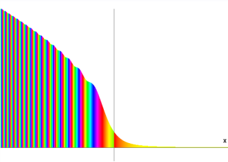
Figure 1: The timeline waveform $\Xi_{\tau}^{\rightarrow}(x)$ for $\tau=-0.005$ constructed from rightward-running plane waves. The shading (coloring) represents varying phase values for this complex function. In units where $\hbar=m=1$, the plot extends from $x=-1$ to $x=+1$. Except for an overall phase factor, this also represents the conjugate of the waveform $\Xi_{\tau}^{\leftarrow}(x)$ at the system time $\tau=0.005$ (cf. Eq.(39)).

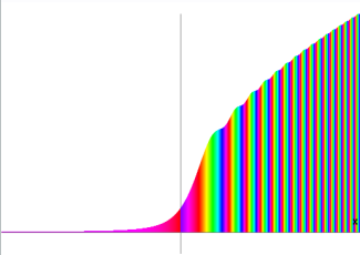
Figure 2: The timeline waveform $\Xi_{\tau}^{\rightarrow}(x)$ for $\tau=0.005$ constructed from rightward-running plane waves. The shading (coloring) represents varying phase values for this complex function. In units where $\hbar=m=1$, the plot extends from $x=-1$ to $x=+1$. Except for an overall phase factor, this also represents the conjugate of the waveform $\Xi_{\tau}^{\leftarrow}(x)$ at the system time $\tau=-0.005$ (cf. Eq.(39)).

V.2 A Free-Particle Time Operator in One Dimension

A time operator for free particles can be constructed following the recipe of Sec. III. The invariance expressed by Eq.(18) ensures that the same time operator results no matter which [degenerate] representation we choose for the computation. With parity as the ‘good’ quantum number, the free-particle time operator is composed from operators in the even- and odd-parity subspaces: $\widehat{T}=\widehat{T}_{+}\oplus\widehat{T}_{-}$, where (cf. Eq.(27))

$$\widehat{T}_{\pm}\equiv P{\displaystyle\int\limits_{-\infty}^{\infty}}|\,\tau,\pm\rangle\tau\langle\,\tau,\pm|\,d\tau$$ (44)

Now the energy-normalized stationary waves of odd parity vanish at the lower spectral bound as $E^{1/4}$(cf. Eq.(36)), so the general theory of Sec. III implies that $\widehat{T}_{-}$ is well-defined by the integral above, the principal value notwithstanding. The coordinate-space matrix elements of this operator are simply related to one of a class of integrals $I_{l}\left(r,r^{\prime}\right)$ studied in Appendix A; using the result reported there, we find

$$\langle\,x\,|\widehat{T}_{-}|\,x^{\prime}\rangle={\displaystyle\int\limits_{-\infty}^{\infty}}\left[\Xi_{\tau}^{-}(x)\right]^{\ast}\tau\Xi_{\tau}^{-}(x^{\prime})\,d\tau=\frac{1}{2}xx^{\prime}I_{0}\left(x,x^{\prime}\right)=i\frac{m}{4}x_{<}\operatorname{sgn}\left(x-x^{\prime}\right)$$ (45)

The case for $\widehat{T}_{+}$ is more delicate, since the energy-normalized stationary waves of even parity actually diverge at the lower spectral bound as $E^{-1/4}$ (cf. Eq.(36)). Nonetheless, Appendix A confirms that the principal value integral for the coordinate space matrix elements of $\widehat{T}_{+}$ remains well-defined, and can be evaluated in closed form to give

$$\langle\,x\,|\widehat{T}_{+}|\,x^{\prime}\rangle={\displaystyle\int\limits_{-\infty}^{\infty}}\left[\Xi_{\tau}^{+}(x)\right]^{\ast}\tau\Xi_{\tau}^{+}(x^{\prime})\,d\tau=\frac{1}{2}xx^{\prime}I_{-1}\left(x,x^{\prime}\right)=i\frac{m}{4}x_{>}\operatorname{sgn}\left(x-x^{\prime}\right)$$ (46)

Combining the even and odd-parity computations, we arrive at the provocatively simple form

$$\langle\,x\,|\widehat{T}_{1d-free}|\,x^{\prime}\rangle=i\frac{m}{4}\left(x+x^{\prime}\right)\operatorname{sgn}\left(x-x^{\prime}\right)$$ (47)

Eq.(47) agrees with the formula reported by Galapon et. al. Galapon for a particle confined to a section of the real line, in the limit where the domain size becomes infinite. Here we arrive at the same result in an unbounded space using an alternative limiting process – the accessible states model.

VI Example: Free Particle in Three Dimensions

In this case, the Hamiltonian $\widehat{H}$ is the operator for kinetic energy in a three-dimensional space. The spectrum of $\widehat{H}$ is semi-infinite (bounded from below by $E=0$, but no upper limit) and composed of degenerate levels. This degeneracy breeds multiple timelines, conveniently indexed by the same quantum numbers that label the spectral states. Again there is some flexibility in labeling here depending upon what dynamical variables we opt to conserve along with particle energy, but the general timeline wave $\langle\,\tau\,|\,\psi\,\rangle$ is constructed from its spectral counterpart $\langle\,E\,|\,\psi\,\rangle$ following the same prescription used in the one-dimensional case, Eq.(34).

VI.1 Angular Momentum Timelines for a Free Particle

In the angular momentum representation, the stationary states are indexed by a continuous wave number $k$ (any non-negative value), an orbital quantum number $l$ (a non-negative integer), and a magnetic quantum number $m_{l}$ (an integer between $-l$ and $+l$, not to be confused with particle mass): $|\,E\,\rangle\rightarrow|\,klm_{l}\,\rangle$. This stationary state has energy $E_{k}=k^{2}/2m$. The associated Schrödinger waveforms are spherical waves $\langle\overrightarrow{r}\,|\,klm_{l}\,\rangle=$ $C_{k}\,\,j_{l}(kr)Y_{l}^{m_{l}}(\Omega_{r})$, formed as a product of a spherical Bessel function $j_{l}$ with a spherical harmonic $Y_{l}^{m_{l}}$. $C_{k}$ is a constant that – for the construction of timelines – is fixed by energy normalization. Noting that the spherical harmonics are themselves normalized over the unit sphere, we apply the Bessel function closure rule Arfken to evaluate the remaining portion of the normalization integral:

$$\langle\,klm_{l}\,|\,k^{\prime}lm_{l}\rangle =C_{k}C_{k^{\prime}}{\displaystyle\int\limits_{0}^{\infty}}\,dr\,r^{2}j_{l}\left(kr\right)j_{l}\left(k^{\prime}r\right)$$

$$=C_{k}^{2}\frac{\pi}{2k^{2}}\,\delta\left(k-k^{\prime}\right)=C_{k}^{2}\,\frac{\pi}{2mk}\,\delta\left(E_{k}\,-\,E_{k}^{\prime}\right)$$

Thus, energy normalization of these spherical waves requires

$$C_{k}=\sqrt{\frac{2mk}{\pi}}$$ (48)

The time states $|\,\tau lm_{l}\rangle$ in this representation have components in the coordinate basis given by $\langle\overrightarrow{r}\,|\,\tau lm_{l}\,\rangle\equiv\Xi_{\tau}^{l}(r)Y_{l}^{m_{l}}(\Omega_{r})$ where $\Xi_{\tau}^{l}(r)$, the radial piece of the timeline wave, is calculated from (cf. Eq.(34)):

$$\Xi_{\tau}^{l}(r) =\frac{1}{\sqrt{2\pi}}{\displaystyle\int\limits_{0}^{\infty}}\exp\left(-iE_{k}\tau\right)\,C_{k}\,j_{l}\left(kr\right)\,dE_{k}$$

$$=\frac{1}{\sqrt{2\pi mr}}{\displaystyle\int\limits_{0}^{\infty}}\exp\left(-ik^{2}\tau/2m\right)\,kJ_{l+1/2}\left(kr\right)\,dk$$ (49)

The last line follows from the connection between spherical Bessel functions and the (cylinder) Bessel functions of the first kind. The closure rule obeyed by these time states

$${\displaystyle\int\limits_{-_{\infty}}^{\infty}}\,\Xi_{\tau}^{l}(r)\,\left[\Xi_{\tau}^{l}(r^{\prime})\right]^{\ast}d\tau=\frac{1}{r^{2}}\,\delta\left(r^{\prime}-r\right)$$

can be confirmed from the integral representation of Eq.(49) using the closure rule for Bessel functions Arfken .

The integral in Eq.(49) converges for all $\Im m\,\tau\leq 0$ and any $l\geq 0$. Defining $2\alpha\equiv l-1/2$, we find Gradshteyn

$$\Xi_{\tau}^{l}(r)=\sqrt{\frac{4r}{m}}z^{3/2}\exp\left(ir^{2}z-i\pi\frac{2\alpha+1}{4}\right)\,\left[J_{\alpha+1}\left(r^{2}z\right)-iJ_{\alpha}\left(r^{2}z\right)\right]\text{\qquad}z\equiv\frac{m}{4\tau}$$ (50)

For fixed $\alpha$, $J_{\alpha}(\ldots)$ is a regular function of its argument throughout the complex plane cut along the negative real axis. Thus, through the magic of analytic continuation, Eq.(50) extends $\Xi_{\tau}^{l}(r)$ to the whole cut $z$-plane$~{}\left|\arg(z)\right|<\pi$. Now for any real $\tau>0$, $z$ is a positive number, say $z=x$. To recover results for $\tau<0$, $z$ must approach the negative real axis from above ($\arg(z)\rightarrow\pi$ for $\arg(\tau)\rightarrow-\pi$). Writing $z=x\exp\left(i\pi\right)$ in Eq.(50) and using $J_{\alpha}(\exp\left(i\pi\right)x)=\exp\left(i\pi\alpha\right)J_{\alpha}(x)$ Bateman leads to the relation

$$\Xi_{-\tau}^{l}(r)=\left[\Xi_{\tau}^{l}(r)\right]^{\ast}$$ (51)

for any real value of $\tau$, a result that also is evident from the integral form, Eq.(49).

The behavior of $\Xi_{\tau}^{l}(r)$ for small $r$ and/or large $\tau$ follows directly from the power series representation of the Bessel function Abramowitz2 . Apart from numerical factors, we find from Eq.(50)

$$\Xi_{\tau}^{l}(r)\simeq\frac{z^{3/2+\alpha}}{r^{5/2}}\,\sim\frac{r^{l}}{\tau^{l/2+5/4}}\text{\qquad}r^{2}\left|z\right|\ll 1$$ (52)

and this result is valid in any sector of the cut $z$-plane. Similarly, the asymptotic series for the Bessel function Abramowitz3 furnishes a large-argument approximation to $\Xi_{\tau}^{l}(r)$, valid for any $l\geq 0$ and $\left|\arg(z)\right|<\pi$:

$$\Xi_{\tau}^{l}(r)\sim\frac{1}{r^{5/2}}\sqrt{\frac{2}{\pi m}}\left[\left(\frac{l\left(l+1\right)+1/4}{4}-i2z\right)\exp\left(i2z-i\pi\frac{2l+1}{4}\right)+\frac{2l+1}{4}\right]\text{\qquad}r^{2}\left|z\right|\gg 1$$ (53)

VI.2 Uni-Directional Timelines for a Free Particle

Free particles also can be described by momentum eigenstates labeled by a wave vector $\overrightarrow{k}$. These momentum states have energy $E_{k}=k^{2}/2m$, and so must be expressible as a superposition of angular momentum states with the same energy:

$$|\,\overrightarrow{k}\,\rangle={\displaystyle\sum_{l=0}^{\infty}}{\displaystyle\sum_{\,m_{l}=-l}^{l}}U_{l}^{m_{l}}\left(\widehat{k}\right)|\,klm_{l}\,\rangle$$ (54)

Here $\widehat{k}$ is the unit vector specifying the orientation of the wave vector with modulus $k$. The transformation from the angular momentum representation to the linear one should be unitary to preserve the energy normalization required for the construction of timelines. To identify the transformation coefficients $U_{l}^{m_{l}}\left(\widehat{k}\right)$, we note first that the Schrödinger waveforms associated with $|\,\overrightarrow{k}\,\rangle$ are plane waves multiplied by a suitable normalizing constant $C_{k}^{(uni)}$:

$$\langle\overrightarrow{r}\,|\,\overrightarrow{k}\,\rangle=C_{k}^{(uni)}\,\,\exp\left(i\overrightarrow{k}\cdot\overrightarrow{r}\right)$$ (55)

Next, we appeal to the spherical wave decomposition of a plane wave Newton

$$\exp\left(i\overrightarrow{k}\cdot\overrightarrow{r}\right)=4\pi{\displaystyle\sum_{l=0}^{\infty}}i^{l}j_{l}(kr){\displaystyle\sum_{\,m_{l}=-l}^{l}}Y_{l}^{m_{l}}(\Omega_{r})\left[Y_{l}^{m_{l}}(\Omega_{k})\right]^{\ast}$$

to write the coordinate-space projection of Eq.(54):

$$4\pi C_{k}^{(uni)}{\displaystyle\sum_{l=0}^{\infty}}i^{l}j_{l}(kr){\displaystyle\sum_{\,m_{l}=-l}^{l}}Y_{l}^{m_{l}}(\Omega_{r})\left[Y_{l}^{m_{l}}(\Omega_{k})\right]^{\ast}={\displaystyle\sum_{l=0}^{\infty}}{\displaystyle\sum_{\,m_{l}=-l}^{l}}U_{l}^{m_{l}}\left(\widehat{k}\right)C_{k}\,\,j_{l}(kr)Y_{l}^{m_{l}}(\Omega_{r})$$

This will be satisfied if for every $l\geq 0$ and $\left|m_{l}\right|\leq l$ we have

$$4\pi C_{k}^{(uni)}i^{l}\left[Y_{l}^{m_{l}}(\Omega_{k})\right]^{\ast}=U_{l}^{m_{l}}\left(\widehat{k}\right)C_{k}\,\,$$

For $l$ and $m_{l}$ both zero this last relation reduces to $\sqrt{4\pi}C_{k}^{(uni)}=U_{0}^{0}\left(\widehat{k}\right)C_{k}$, leaving $\sqrt{4\pi}U_{0}^{0}\left(\widehat{k}\right)i^{l}\left[Y_{l}^{m_{l}}(\Omega_{k})\right]^{\ast}=U_{l}^{m_{l}}\left(\widehat{k}\right)$. Setting $\sqrt{4\pi}U_{0}^{0}\left(\widehat{k}\right)=1$ then leads to

$$U_{l}^{m_{l}}\left(\widehat{k}\right)=i^{l}\left[Y_{l}^{m_{l}}(\Omega_{k})\right]^{\ast}$$ (56)

that describes the desired unitary transformation Arfken4 :

$${\displaystyle\sum_{l=0}^{\infty}}{\displaystyle\sum_{\,m_{l}=-l}^{l}}U_{l}^{m_{l}}\left(\widehat{k_{2}}\right)\left[U_{l}^{m_{l}}\left(\widehat{k_{1}}\right)\right]^{\ast}={\displaystyle\sum_{l=0}^{\infty}}{\displaystyle\sum_{\,m_{l}=-l}^{l}}\left[Y_{l}^{m_{l}}(\Omega_{2})\right]^{\ast}Y_{l}^{m_{l}}(\Omega_{1})=\delta\left(\Omega_{1}\,-\,\Omega_{2}\right)$$

It follows that the energy-normalized plane waves are described by the normalizing factor

$$C_{k}^{(uni)}=\frac{C_{k}}{\sqrt{4\pi}}U_{0}^{0}\left(\widehat{k}\right)=\frac{1}{4\pi}\sqrt{\frac{2mk}{\pi}}$$ (57)

Uni-directional time states are formed from plane waves all moving in the same direction, but with differing energy. Accordingly, we adopt the unit vector $\widehat{k}$ as an additional label for such time states, writing $|\,\tau\,\rangle\rightarrow|\,\tau,\widehat{k}\,\rangle$. These uni-directional time states can be related to the angular momentum time states of the preceding section. Combining Eqs.(34), (54), and (56), we find that the uni-directional timeline wave in the coordinate basis, $\langle\overrightarrow{r}\,|\,\tau,\widehat{k}\,\rangle\equiv\Xi_{\tau}^{\widehat{k}\,}(\overrightarrow{r})$, can be computed from the spherical-wave expansion

$$\Xi_{\tau}^{\widehat{k}\,}(\overrightarrow{r})={\displaystyle\sum_{l=0}^{\infty}}i^{l}\Xi_{\tau}^{l}(r){\displaystyle\sum_{\,m_{l}=-l}^{l}}Y_{l}^{m_{l}}(\Omega_{r})\left[Y_{l}^{m_{l}}(\Omega_{k})\right]^{\ast},$$ (58)

where $\Xi_{\tau}^{l}(r)$ is the radial timeline wave of Eq.(50).

Alternatively, we might try to calculate $\Xi_{\tau}^{\widehat{k}\,}(\overrightarrow{r})$ directly by taking $|\,\psi\,\rangle=|\,\overrightarrow{r}\,\rangle$ in Eq.(34). With the help of Eqs.(55) and (57), we obtain in this way

$$\Xi_{\tau}^{\widehat{k}\,}(\overrightarrow{r}) =\frac{1}{\sqrt{2\pi}}{\displaystyle\int\limits_{0}^{\infty}}\exp\left(-iE_{k}\tau\right)\,\langle\,\overrightarrow{r}\,|\,\overrightarrow{k}\,\rangle\,dE_{k}$$

$$=\frac{1}{4\pi^{2}\sqrt{m}}{\displaystyle\int\limits_{0}^{\infty}}\exp\left(-ik^{2}\tau/2m+i\,k\widehat{k}\cdot\overrightarrow{r}\right)\,k^{3/2}\,dk$$ (59)

Eq.(59) shows that the dependence of $\Xi_{\tau}^{\widehat{k}\,}(\overrightarrow{r})$ on $\widehat{k}$ and on $\overrightarrow{r}$ occurs only through the combination $\xi\equiv\widehat{k}\cdot\overrightarrow{r}$, which is nothing more than the projection of the coordinate vector $\overrightarrow{r}$ onto the direction of plane wave propagation. (Indeed, $\Xi_{\tau}^{\widehat{k}\,}(\overrightarrow{r})$ itself is a plane wave – albeit not a harmonic one – with the surfaces of constant wave amplitude oriented perpendicular to $\widehat{k}$.) In terms of $\xi$, then, there is a universal timeline applicable to any direction in space, as befits the expected isotropy of a free-particle environment. This universal timeline has elements that we denote simply as $\Xi_{\tau}^{\,}(\xi)$, and are given by

$$\Xi_{\tau}^{\,}(\xi)=\frac{1}{4\pi^{2}\sqrt{m}}{\displaystyle\int\limits_{0}^{\infty}}\exp\left(-ik^{2}\tau/2m+i\,k\xi\right)\,k^{3/2}\,dk$$ (60)

Unlike a similar integral encountered in the one-dimensional case, Eq.(60) fails to converge for real values of $\tau$. But the integral does define a function that is analytic throughout the lower half plane $\Im m\,\tau<0$, and can be analytically continued onto the real axis. For $\Re e\left(\,i\tau\right)>0$ we have Gradshteyn2

$$\Xi_{\tau}^{\,}(\xi)=\frac{3}{16\sqrt{\pi^{3}m}}z^{5/2}\exp\left(-\xi^{2}z^{2}/4\right)D_{-5/2}\left(-i\xi z\right)\text{\qquad}z\equiv\sqrt{\frac{m}{i\tau}},$$ (61)

where $D_{-5/2}\left(\ldots\right)$ is another of the parabolic cylinder functions. Eq.(61) limits $\tau$ to the sector $-\pi<\arg\,\tau<0$ ($\Re e\left(\,i\tau\right)>0$), but the mapping from $z$ to $\tau$ allows analytic continuation to the whole $\tau$-plane cut along the negative real axis, $-\pi\leq\arg\,\tau<\pi$. The complex variable $z$ then is mapped into the sector $-3\pi/4<\arg\,z\leq\pi/4$. And because $D_{\nu}$ is an entire function of its argument Bateman2 , Eq.(61) defines a single-valued function throughout this domain. Comparing Eq.(61) for $\tau>0$ ($\arg\,z=-\pi/4$) and $\tau<0$ ($\arg\,z=\pi/4$), we discover for all real values of $\xi$ and $\tau$

$$\Xi_{\tau}(\xi)=\left[\Xi_{-\tau}(-\xi)\right]^{\ast}$$ (62)

For $\tau>0$ ($\arg\,z=-\pi/4$), the asymptotics of the parabolic cylinder function Bateman3 imply

$$\Xi_{\tau}(\xi)\sim\begin{array}[c]{cc}\exp\left(im\xi^{2}/2\tau\right)\xi^{3/2}&\qquad\xi>0\\ \left|\xi\right|^{-5/2}&\qquad\xi<0\end{array}$$

Thus, $\Xi_{\tau}(\xi)$ diverges as $\xi^{3/2}$ for $\xi\rightarrow\infty$ and vanishes as $\left|\xi\right|^{-5/2}$ for $\xi\rightarrow-\infty$. Analogous results for $\tau<0$ follow from Eq.(62). The behavior is reminiscent of the timeline functions constructed from running waves in one dimension. Indeed, it appears that in $\Xi_{\tau}(\xi)$ we again have time-of-arrival functions, with $-\tau$ denoting the arrival time at the coordinate origin for waves moving in the direction of $\widehat{k}$, and $\xi\equiv\widehat{k}\cdot\overrightarrow{r}$. This interpretation is supported by the illustrations in Figs. 3 and 4 showing $\Xi_{\tau}(\xi)$ for system times just prior to, and immediately following, arrival at the coordinate origin.

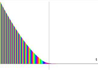
Figure 3: The universal timeline waveform $\Xi_{\tau}(\xi)$ for the system time $\tau=-0.005$. The shading (coloring) represents varying phase values for this complex function. In units where $\hbar=m=1$, the plot extends from $\xi=-1$ to $\xi=+1$.

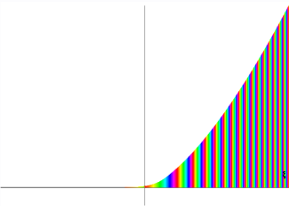
Figure 4: The universal timeline waveform $\Xi_{\tau}(\xi)$ for the system time $\tau=+0.005$. The shading (coloring) represents varying phase values for this complex function. In units where $\hbar=m=1$, the plot extends from $\xi=-1$ to $\xi=+1$.

VI.3 The Three-Dimensional Free-Particle Time Operator

Lastly, we investigate the time operator for this example. We exercise the freedom allowed by the degeneracy of free particle states to work in the angular momentum representation. From Eq.(48) we find that the stationary spherical waves $\langle\overrightarrow{r}\,|\,klm_{l}\,\rangle=C_{k}\,\,j_{l}(kr)Y_{l}^{m_{l}}(\Omega_{r})$ vanish at the lower spectral edge ($\lim_{k\rightarrow 0}\langle\overrightarrow{r}\,|\,klm_{l}\,\rangle=0$), so that a free-particle time operator in three space dimensions does exist by the theory of Sec. III. The matrix elements of $\widehat{T}$ in the coordinate basis are given by (cf. Eq.(19))

$$\langle\,\overrightarrow{r_{1}}\,|\widehat{T}_{3d-free}|\,\overrightarrow{r_{2}}\,\rangle ={\displaystyle\sum_{l,\,m_{l}}}P{\displaystyle\int\limits_{-\infty}^{\infty}}\langle\,\overrightarrow{r_{1}}\,|\,\tau lm_{l}\rangle\tau\langle\tau lm_{l}\,|\,\overrightarrow{r_{2}}\,\rangle\,d\tau$$

$$={\displaystyle\sum_{l,\,m_{l}}}Y_{l}^{m_{l}}(\Omega_{1})\left[Y_{l}^{m_{l}}(\Omega_{2})\right]^{\ast}P{\displaystyle\int\limits_{-\infty}^{\infty}}\tau\,\Xi_{\tau}^{l}(r_{1})\left[\Xi_{\tau}^{l}(r_{2})\right]^{\ast}\,d\tau$$

The principal value integrals are studied in Appendix A, where their existence is rigorously established and a closed-form expression given for their evaluation:

$$P{\displaystyle\int\limits_{-\infty}^{\infty}}\tau\,\Xi_{\tau}^{l}(r_{1})\left[\Xi_{\tau}^{l}(r_{2})\right]^{\ast}\,d\tau=i\frac{m}{2}\operatorname{sgn}\left(r_{1}-r_{2}\right)\frac{1}{r_{>}}\left(\frac{r_{<}}{r_{>}}\right)^{l}$$

Collecting the above results, we obtain

$$\langle\,\overrightarrow{r_{1}}\,|\widehat{T}_{3d-free}|\,\overrightarrow{r_{2}}\,\rangle=i\frac{m}{2}\operatorname{sgn}\left(r_{1}-r_{2}\right)\frac{1}{r_{>}}{\displaystyle\sum_{l,\,m_{l}}}Y_{l}^{m_{l}}(\Omega_{1})\left[Y_{l}^{m_{l}}(\Omega_{2})\right]^{\ast}\left(\frac{r_{<}}{r_{>}}\right)^{l}$$

The remaining sums also can be evaluated in closed form. Combining the generating function for the Legendre polynomials Arfken2 with the addition theorem for spherical harmonics Arfken3 , we obtain for any $\left|t\right|<1$

$$\frac{1}{\sqrt{1-2t\cos\gamma+t^{2}}} ={\displaystyle\sum_{l=0}^{\infty}}P_{l}(\cos\gamma)t^{l}$$

$$=4\pi{\displaystyle\sum_{l=0}^{\infty}}{\displaystyle\sum_{\,m_{l}=-l}^{l}}Y_{l}^{m_{l}}(\Omega_{1})\left[Y_{l}^{m_{l}}(\Omega_{2})\right]^{\ast}\frac{t^{l}}{2l+1},$$

from which it follows that

$$2\pi{\displaystyle\sum_{l=0}^{\infty}}{\displaystyle\sum_{\,m_{l}=-l}^{l}}Y_{l}^{m_{l}}(\Omega_{1})\left[Y_{l}^{m_{l}}(\Omega_{2})\right]^{\ast}t^{l} =t^{1/2}\frac{\partial}{\partial t}\left(\frac{t^{1/2}}{\sqrt{1-2t\cos\gamma+t^{2}}}\right)$$

$$=\frac{1-t^{2}}{2\left(1-2t\cos\gamma+t^{2}\right)^{3/2}}$$

Finally, identifying $t$ with $r_{<}/r_{>}$ gives

$$\langle\,\overrightarrow{r_{1}}\,|\widehat{T}_{3d-free}|\,\overrightarrow{r_{2}}\,\rangle =i\frac{m}{2}\operatorname{sgn}\left(r_{1}-r_{2}\right)\frac{1}{4\pi}\frac{r_{>}^{2}-r_{<}^{2}}{\left(r_{>}^{2}-2r_{<}r_{>}\cos\gamma+r_{<}^{2}\right)^{3/2}}$$

$$=\frac{im}{8\pi}\frac{\overrightarrow{r_{1}}\cdot\overrightarrow{r_{1}}-\overrightarrow{r_{2}}\cdot\overrightarrow{r_{2}}}{\,\left|\overrightarrow{r_{1}}-\overrightarrow{r_{2}}\right|^{3}}=\frac{im}{8\pi}\frac{\left(\overrightarrow{r_{1}}-\overrightarrow{r_{2}}\right)}{\,\left|\overrightarrow{r_{1}}-\overrightarrow{r_{2}}\right|^{3}}\cdot\left(\overrightarrow{r_{1}}+\overrightarrow{r_{2}}\right)$$ (63)

The vector form for these matrix elements is pleasingly compact, and frees the result from the spherical coordinates adopted for the computation.

It is apparent that Eq.(63) specifies matrix elements of a Hermitian operator, i.e., $\langle\,\overrightarrow{r_{1}}\,|\widehat{T}_{3d-free}|\,\overrightarrow{r_{2}}\,\rangle=\langle\,\overrightarrow{r_{2}}\,|\widehat{T}_{3d-free}|\,\overrightarrow{r_{1}}\,\rangle^{\ast}$ for $\overrightarrow{r_{1}}\neq\overrightarrow{r_{2}}$. That these matrix elements also specify an operator that is canonically conjugate to the free-particle Hamiltonian is confirmed in Appendix B. Thus, a canonical time operator for a free particle in three dimensions exists, with coordinate-space matrix elements given by Eq.(63).

VII Summary and Conclusions

Contrary to conventional wisdom, we contend that [event] time is a legitimate observable, and fits within the framework of standard quantum theory if we extend the latter to include POVM’s – and not just self-adjoint operators – for representing observables. This modest change in emphasis places the focus squarely on probability amplitudes, in keeping with the seemingly evident fact that [event] time statistics can be generated empirically for virtually any quantum system. As with every other observable, we show these [event] time statistics derive from wave functions expressed in a suitable basis (the time basis), which is complete for the representation of any physical state. We refer to this basis as a timeline, or quantum history, with elements labeled by a continuous variable we call the system time. While time states are typically not orthogonal, they do lead to wave functions and statistics that are covariant (time-translation invariant), and probabilities that add to unity. We propose a recipe for calculating wave functions in the time basis from those in the spectral basis. This recipe is dictated solely by the demands of covariance and completeness, and applies to virtually any Hamiltonian system. The phase ambiguity inherent in the stationary states translates here into a freedom to construct time statistics pertinent to different kinds of events.

The leap from time states to a time operator is non-trivial, involving additional assumptions that are not always met. Indeed, it is the nature of time statistics that they need not admit a well-defined mean, or variance. Time operators – when they exist – are system specific, useful for calculating moments of the [event] time distribution in those instances where said moments can be shown to converge. Interestingly, we find that time operators for periodic systems are never canonical to the Hamiltonian, but canonical time operators can and do arise in [aperiodic] systems with a vanishing point spectrum (no isolated levels).

As examples of these general principles, we have examined several systems (particle in free-fall, free particle in one dimension) for which results have been reported previously in the literature. Our objective has been to illustrate how these diverse results follow from the unified approach developed here. We also have gone beyond the familiar and applied that same approach to the free particle in three dimensions. To the best of our knowledge, results for the latter have never before appeared. Most importantly, they confirm that the notion of an arrival time – first encountered in the one-dimensional case – extends to three dimensions, complete with an accompanying canonical time operator. Possibilities for future investigations abound. For instance, how to generate correct arrival-time statistics for a particle scattering from even the simplest one-dimensional barrier remains a subject of controversy Baute ; we expect that discussion – and numerous others – to be informed by the results presented here.

Appendix A Time Operators and The Integrals $I_{l}\left(r_{1},r_{2}\right)$

In this Appendix we investigate the principal value integrals that arise in the construction of a canonical time operator for free particles:

$$I_{l}\left(r_{1},r_{2}\right)\equiv P{\displaystyle\int\limits_{-\infty}^{\infty}}\tau\,\Xi_{\tau}^{l}(r_{1})\left[\Xi_{\tau}^{l}(r_{2})\right]^{\ast}\,d\tau\equiv\lim_{\tau_{R}\rightarrow\infty}{\displaystyle\int\limits_{-\tau_{R}}^{+\tau_{R}}}\tau\,\Xi_{\tau}^{l}(r_{1})\left[\Xi_{\tau}^{l}(r_{2})\right]^{\ast}\,d\tau$$ (64)

Here $\Xi_{\tau}^{l}(r)$ is the timeline wavefunction in the $l^{th}$ angular momentum subspace, given by Eq.(50). Inspection of Eqs.(42) and (43) shows that the $l=-1$ and $l=0$ integrals also appear in the context of the time operator for a free particle in one dimension. Our objective here is to establish the existence of these integrals, and obtain closed-form expressions suitable for their evaluation.

The relation $\Xi_{-\tau}^{l}(r)=\left[\Xi_{\tau}^{l}(r)\right]^{\ast}$ can be used to show that $I_{l}\left(r_{1},r_{2}\right)$ is purely imaginary, as well as antisymmetric under the interchange $r_{1}\longleftrightarrow r_{2}$, properties that can be used to reduce the integral to the half-axis $\tau\geq 0$:

$$I_{l}\left(r_{1},r_{2}\right)=2i\,\Im m\left[\lim_{\tau_{R}\rightarrow\infty}{\displaystyle\int\limits_{0}^{\tau_{R}}}\tau\,\Xi_{\tau}^{l}(r_{1})\left[\Xi_{\tau}^{l}(r_{2})\right]^{\ast}\,d\tau\right]$$ (65)

Substituting from Eq.(50), this becomes (recall $2\alpha\equiv l-1/2$)

$$I_{l}\left(r_{1},r_{2}\right)=i\frac{m\sqrt{r_{1}r_{2}}}{2}\left(I_{1}+I_{2}\right)$$

where

$$I_{1} \equiv\lim_{s_{R}\rightarrow 0^{+}}{\displaystyle\int\limits_{s_{R}}^{\infty}}\sin\left(s\left[r_{1}^{2}-r_{2}^{2}\right]\right)\left[J_{\alpha+1}\left(s\,r_{1}^{2}\right)J_{\alpha+1}\left(s\,r_{2}^{2}\right)+J_{\alpha}\left(s\,r_{1}^{2}\right)J_{\alpha}\left(s\,r_{2}^{2}\right)\right]\,ds$$

$$I_{2} \equiv\lim_{s_{R}\rightarrow 0^{+}}{\displaystyle\int\limits_{s_{R}}^{\infty}}\cos\left(s\left[r_{1}^{2}-r_{2}^{2}\right]\right)\left[J_{\alpha+1}\left(s\,r_{1}^{2}\right)J_{\alpha}\left(s\,r_{2}^{2}\right)-J_{\alpha}\left(s\,r_{1}^{2}\right)J_{\alpha+1}\left(s\,r_{2}^{2}\right)\right]\,ds$$

The small-argument behavior of $J_{\alpha}$ ensures that both integrals exist in the indicated limits provided $\alpha>-1$: accordingly, explicit reference to the limits will be omitted from subsequent expressions.

Our next goal is to relate $I_{2}$ to $I_{1}$. To that end we define the related (and simpler) integrals $\widetilde{I}_{1,2}$ by

$$\widetilde{I}_{1}^{\alpha}\left(r_{1},r_{2}\right) \equiv{\displaystyle\int\limits_{0}^{\infty}}\sin\left(s\left[r_{1}^{2}-r_{2}^{2}\right]\right)J_{\alpha}\left(s\,r_{1}^{2}\right)J_{\alpha}\left(s\,r_{2}^{2}\right)\,ds$$

$$\widetilde{I}_{2}^{\alpha}\left(r_{1},r_{2}\right) \equiv{\displaystyle\int\limits_{0}^{\infty}}\cos\left(s\left[r_{1}^{2}-r_{2}^{2}\right]\right)J_{\alpha+1}\left(s\,r_{1}^{2}\right)J_{\alpha}\left(s\,r_{2}^{2}\right)\,ds$$

Then $I_{1}\equiv\widetilde{I}_{1}^{\alpha+1}\left(r_{1},r_{2}\right)+\widetilde{I}_{1}^{\alpha}\left(r_{1},r_{2}\right)$ and $I_{2}\equiv\widetilde{I}_{2}^{\alpha}\left(r_{1},r_{2}\right)-\widetilde{I}_{2}^{\alpha}\left(r_{2},r_{1}\right)$. Integrating $\widetilde{I}_{2}$ once by parts (the out-integrated part vanishes for $\alpha>-1$) and using the Bessel recursion relation Bateman

$$J_{\nu-1}\left(z\right)-J_{\nu+1}\left(z\right)=2\frac{dJ_{\nu}\left(z\right)}{dz}$$

results in

$$\widetilde{I}_{2}^{\alpha}\left(r_{1},r_{2}\right) =-\frac{1}{r_{1}^{2}-r_{2}^{2}}{\displaystyle\int\limits_{0}^{\infty}}\sin\left(s\left[r_{1}^{2}-r_{2}^{2}\right]\right)\frac{\partial}{\partial s}\left[J_{\alpha+1}\left(s\,r_{1}^{2}\right)J_{\alpha}\left(s\,r_{2}^{2}\right)\right]\,ds$$

$$=\frac{r_{2}^{2}}{2\left(r_{1}^{2}-r_{2}^{2}\right)}{\displaystyle\int\limits_{0}^{\infty}}\sin\left(s\left[r_{1}^{2}-r_{2}^{2}\right]\right)J_{\alpha+1}\left(s\,r_{1}^{2}\right)\left[J_{\alpha+1}\left(s\,r_{2}^{2}\right)-J_{\alpha-1}\left(s\,r_{2}^{2}\right)\right]\,ds$$

$$+\frac{r_{1}^{2}}{2\left(r_{1}^{2}-r_{2}^{2}\right)}{\displaystyle\int\limits_{0}^{\infty}}\sin\left(s\left[r_{1}^{2}-r_{2}^{2}\right]\right)J_{\alpha}\left(s\,r_{2}^{2}\right)\left[J_{\alpha+2}\left(s\,r_{1}^{2}\right)-J_{\alpha}\left(s\,r_{1}^{2}\right)\right]\,ds$$

In terms of yet a third integral $\widetilde{I}_{3}$ defined as

$$\widetilde{I}_{3}^{\alpha}\left(r_{1},r_{2}\right) \equiv{\displaystyle\int\limits_{0}^{\infty}}\sin\left(s\left[r_{1}^{2}-r_{2}^{2}\right]\right)J_{\alpha+1}\left(s\,r_{1}^{2}\right)J_{\alpha-1}\left(s\,r_{2}^{2}\right)\,ds$$

$$=\frac{2\alpha}{r_{2}^{2}}{\displaystyle\int\limits_{0}^{\infty}}\sin\left(s\left[r_{1}^{2}-r_{2}^{2}\right]\right)J_{\alpha+1}\left(s\,r_{1}^{2}\right)J_{\alpha}\left(s\,r_{2}^{2}\right)\,\frac{ds}{s}-\widetilde{I}_{1}^{\alpha+1}\left(r_{1},r_{2}\right)$$

$$=\frac{2\alpha}{r_{1}^{2}}{\displaystyle\int\limits_{0}^{\infty}}\sin\left(s\left[r_{1}^{2}-r_{2}^{2}\right]\right)J_{\alpha}\left(s\,r_{1}^{2}\right)J_{\alpha-1}\left(s\,r_{2}^{2}\right)\,\frac{ds}{s}-\widetilde{I}_{1}^{\alpha-1}\left(r_{1},r_{2}\right)$$

we can write the result for $\widetilde{I}_{2}$ compactly as

$$\widetilde{I}_{2}^{\alpha}\left(r_{1},r_{2}\right) =\frac{1}{2\left(r_{1}^{2}-r_{2}^{2}\right)}\left[-r_{1}^{2}\widetilde{I}_{1}^{\alpha}\left(r_{1},r_{2}\right)+r_{2}^{2}\widetilde{I}_{1}^{\alpha+1}\left(r_{1},r_{2}\right)-r_{2}^{2}\widetilde{I}_{3}^{\alpha}\left(r_{1},r_{2}\right)+r_{1}^{2}\widetilde{I}_{3}^{\alpha+1}\left(r_{1},r_{2}\right)\right]$$

$$=\frac{1}{\left(r_{1}^{2}-r_{2}^{2}\right)}\left[-r_{1}^{2}\widetilde{I}_{1}^{\alpha}\left(r_{1},r_{2}\right)+r_{2}^{2}\widetilde{I}_{1}^{\alpha+1}\left(r_{1},r_{2}\right)+{\displaystyle\int\limits_{0}^{\infty}}\sin\left(s\left[r_{1}^{2}-r_{2}^{2}\right]\right)J_{\alpha+1}\left(s\,r_{1}^{2}\right)J_{\alpha}\left(s\,r_{2}^{2}\right)\,\frac{ds}{s}\right]$$

Then

$$I_{2} =\frac{1}{\left(r_{1}^{2}-r_{2}^{2}\right)}\left[-r_{1}^{2}\widetilde{I}_{1}^{\alpha}\left(r_{1},r_{2}\right)+r_{2}^{2}\widetilde{I}_{1}^{\alpha+1}\left(r_{1},r_{2}\right)+r_{2}^{2}\widetilde{I}_{1}^{\alpha}\left(r_{1},r_{2}\right)-r_{1}^{2}\widetilde{I}_{1}^{\alpha+1}\left(r_{1},r_{2}\right)\right]$$

$$+\frac{1}{\left(r_{1}^{2}-r_{2}^{2}\right)}{\displaystyle\int\limits_{0}^{\infty}}\sin\left(s\left[r_{1}^{2}-r_{2}^{2}\right]\right)\left[J_{\alpha+1}\left(s\,r_{1}^{2}\right)J_{\alpha}\left(s\,r_{2}^{2}\right)-J_{\alpha+1}\left(s\,r_{2}^{2}\right)J_{\alpha}\left(s\,r_{1}^{2}\right)\right]\,\frac{ds}{s}$$

$$=-I_{1}+\frac{1}{\left(r_{1}^{2}-r_{2}^{2}\right)}{\displaystyle\int\limits_{0}^{\infty}}\sin\left(s\left[r_{1}^{2}-r_{2}^{2}\right]\right)\left[J_{\alpha+1}\left(s\,r_{1}^{2}\right)J_{\alpha}\left(s\,r_{2}^{2}\right)-J_{\alpha+1}\left(s\,r_{2}^{2}\right)J_{\alpha}\left(s\,r_{1}^{2}\right)\right]\,\frac{ds}{s}$$

and so

$$I_{l}\left(r_{1},r_{2}\right)=i\frac{m\sqrt{r_{1}r_{2}}}{2\left(r_{1}^{2}-r_{2}^{2}\right)}{\displaystyle\int\limits_{0}^{\infty}}\sin\left(s\left[r_{1}^{2}-r_{2}^{2}\right]\right)\left[J_{\alpha+1}\left(s\,r_{1}^{2}\right)J_{\alpha}\left(s\,r_{2}^{2}\right)-J_{\alpha+1}\left(s\,r_{2}^{2}\right)J_{\alpha}\left(s\,r_{1}^{2}\right)\right]\,\frac{ds}{s}$$ (66)

Finally, from integral tables Gradshteyn3 we have for $a,b>0$ and $\alpha>-1$:

$${\displaystyle\int\limits_{0}^{\infty}}J_{\alpha+1}\left(ax\right)J_{\alpha}\left(bx\right)\sin\left(cx\right)\,\frac{dx}{x} =0\text{ \ \ \ for }0<c<b-a$$

$$=a^{-\alpha-1}b^{\alpha}c\text{ \ \ for }0<c<a-b$$

This result is applied separately to each integral in Eq.(66). In terms of the smaller ($r_{<}$) and larger ($r_{>}$) of its two arguments, the final form for $I_{l}\left(r_{1},r_{2}\right)$ can be written most compactly as

$$I_{l}\left(r_{1},r_{2}\right)=i\frac{m}{2}\operatorname{sgn}\left(r_{1}-r_{2}\right)\frac{1}{r_{>}}\left(\frac{r_{<}}{r_{>}}\right)^{l}$$ (67)

Appendix B Canonical Property of the Free-Particle Time Operator in Three Dimensions

In this Appendix we establish that the time operator of Eq.(63) is canonical to the free-particle Hamiltonian $\widehat{H}=\widehat{p}^{2}/2m$. To that end we examine the coordinate-space matrix elements of the commutator

$$\langle\,\overrightarrow{r_{1}}\,|\left[\widehat{T}_{3d-free},\widehat{H}\right]|\,\overrightarrow{r_{2}}\,\rangle =\frac{1}{2m}\langle\,\overrightarrow{r_{1}}\,|\widehat{T}_{3d-free}\widehat{p}^{2}-\widehat{p}^{2}\widehat{T}_{3d-free}|\,\overrightarrow{r_{2}}\,\rangle$$

$$=\frac{1}{2m}\left(\nabla_{1}^{2}-\nabla_{2}^{2}\right)\langle\,\overrightarrow{r_{1}}\,|\widehat{T}_{3d-free}|\,\overrightarrow{r_{2}}\,\rangle$$ (68)

For evaluating the Laplacians in this expression, we apply the vector calculus identity Griffiths

$$\nabla\left(\overrightarrow{A}\cdot\overrightarrow{B}\right)=\overrightarrow{A}\times\left(\nabla\times\overrightarrow{B}\right)+\overrightarrow{B}\times\left(\nabla\times\overrightarrow{A}\right)+\left(\overrightarrow{A}\cdot\nabla\right)\overrightarrow{B}+\left(\overrightarrow{B}\cdot\nabla\right)\overrightarrow{A}$$ (69)

with the identifications

$$\overrightarrow{A}=\frac{\left(\overrightarrow{r_{1}}-\overrightarrow{r_{2}}\right)}{\,\left|\overrightarrow{r_{1}}-\overrightarrow{r_{2}}\right|^{3}};\quad\overrightarrow{B}=\overrightarrow{r_{1}}+\overrightarrow{r_{2}}$$

Noting that $\overrightarrow{A}$ is essentially the electrostatic field of a point charge, we have

$$\nabla_{1}\cdot\overrightarrow{A} =4\pi\,\delta\left(\overrightarrow{r_{1}}-\overrightarrow{r_{2}}\right)=-\nabla_{2}\cdot\overrightarrow{A}$$

$$\nabla_{1}\times\overrightarrow{A} =0=\nabla_{2}\times\overrightarrow{A}$$

$\overrightarrow{B}$ also is curl-free, so the first two terms in Eq.(69) are zero. Further, with $\overrightarrow{r_{1,2}}=\left(x_{1,2},\,y_{1,2},\,z_{1,2}\right)$, the simplicity of $\overrightarrow{B}$ allows us to write

$$\left(\overrightarrow{A}\cdot\nabla_{1}\right)B_{x} =\left(A_{x}\frac{\partial}{\partial x_{1}}+A_{y}\frac{\partial}{\partial y_{1}}+A_{z}\frac{\partial}{\partial z_{1}}\right)\left(x_{1}+x_{2}\right)$$

$$=A_{x},\text{ \ etc.}$$

and

$$\frac{\partial}{\partial x_{1}}\left[\left(\overrightarrow{B}\cdot\nabla_{1}\right)A_{x}\right] =\frac{\partial}{\partial x_{1}}\left[\left(x_{1}+x_{2}\right)\frac{\partial A_{x}}{\partial x_{1}}+\left(y_{1}+y_{2}\right)\frac{\partial A_{x}}{\partial y_{1}}+\left(z_{1}+z_{2}\right)\frac{\partial A_{x}}{\partial z_{1}}\right]$$

$$=\left(\overrightarrow{B}\cdot\nabla_{1}\right)\frac{\partial A_{x}}{\partial x_{1}}+\frac{\partial A_{x}}{\partial x_{1}},\text{ \ etc.}$$

Then

$$\nabla_{1}^{2}\left(\overrightarrow{A}\cdot\overrightarrow{B}\right)=\nabla_{1}\cdot\nabla_{1}\left(\overrightarrow{A}\cdot\overrightarrow{B}\right)=2\left(\nabla_{1}\cdot\overrightarrow{A}\right)+\left(\overrightarrow{B}\cdot\nabla_{1}\right)\left(\nabla_{1}\cdot\overrightarrow{A}\right)$$ (70)

Replacing $\nabla_{1}$ with $\nabla_{2}$ in this last expression generates an equally valid result, but since $\overrightarrow{A}$ depends only on $\overrightarrow{r_{1}}-\overrightarrow{r_{2}}$, we obtain

$$\nabla_{2}^{2}\left(\overrightarrow{A}\cdot\overrightarrow{B}\right)=-2\left(\nabla_{1}\cdot\overrightarrow{A}\right)+\left(\overrightarrow{B}\cdot\nabla_{1}\right)\left(\nabla_{1}\cdot\overrightarrow{A}\right)$$ (71)

and finally,

$$\langle\,\overrightarrow{r_{1}}\,|\left[\widehat{T}_{3d-free},\widehat{H}\right]|\,\overrightarrow{r_{2}}\,\rangle =i\frac{1}{16\pi}\left(\nabla_{1}^{2}-\nabla_{2}^{2}\right)\left(\overrightarrow{A}\cdot\overrightarrow{B}\right)$$

$$=i\frac{1}{4\pi}\,\left(\nabla_{1}\cdot\overrightarrow{A}\right)=i\,\delta\left(\overrightarrow{r_{1}}-\overrightarrow{r_{2}}\right)$$ (72)

We conclude that $\left[\widehat{T}_{3d-free},\widehat{H}\right]=i$, i.e., that $\widehat{T}_{3d-free}$ is canonical to the free-particle Hamiltonian $\widehat{H}$.

References

- (1) W. Pauli in Handbuch der Physik (Springer, Berlin, 1933), Vol. 24 p. 83.
- (2) Time in Quantum Mechanics -Vol. 1 (Lec. Notes Phys. 734), 2nd ed. edited by G. Muga, R.S. Mayato, and I. Egusquiza (Springer, Berlin Heidelberg 2008).
- (3) Time in Quantum Mechanics -Vol. 2 (Lec. Notes Phys. 789) edited by G. Muga, A. Ruschhaupt, and A. del Campo (Springer, Berlin Heidelberg 2009).
- (4) M.D. Srinivas and R. Vijayalakshmi, Pramana 16, 173 (1981).
- (5) J. Kijowski, Rep. Math. Phys. 6, 362 (1974).
- (6) D.T. Pegg, Phys. Rev. A 58, 4307 (1998).
- (7) See for example, Peter J. Olver, Introduction to Partial Differential Equations, (University of Minnesota, 2010), p 97-8.
- (8) E. Merzbacher, Quantum Mechanics, 2nd ed. (John Wiley & Sons, New York, 1970), p 86.
- (9) We expect that grows without bound as increases, implying that there is no natural upper limit to the energy spectrum. While this may seem evident on its face, there exist model spectra for which it is not true (e.g., the discrete spectrum of atomic hydrogen).
- (10) C.W. Helstrom, Quantum Detection and Estimation Theory (Academic Press, New York, 1976), pp. 53–80.
- (11) For an in-depth discussion of this point see G.C. Hegerfeldt, D. Seidel, J.G. Muga, and B. Navarro, Phys. Rev. A 70, 012110 (2004), and references therein.
- (12) R. Giannitrapani, Int. J. Theor. Phys. 36, 1575 (1997).
- (13) A. Erdélyi, Asymptotic Expansions (Dover Publications Inc., New York, 1956), p. 47.
- (14) Peter J. Olver, Introduction to Partial Differential Equations, (University of Minnesota, 2010), p 301.
- (15) L.D. Landau and E.M. Lifshitz, Quantum Mechanics, 2nd ed. (Pergamon Press, Oxford, 1965), p. 269.
- (16) D.E. Aspnes, Physical Review 147, 554 (1966).
- (17) Handbook of Mathematical Functions edited by M. Abramowitz and I. A. Stegun, (Dover, New York, 1965), p. 447.
- (18) I.S. Gradshteyn and I.M. Ryzhik, Table of Integrals, Series, and Products, 4th ed. (Academic Press, New York,1965), p. 337.
- (19) Higher Transcendental Functions Vol. II edited by A. Erdélyi, (McGraw-Hill, New York, 1953), p.117.
- (20) J.G. Muga, C.R. Leavens, and J.P. Palao, Phys. Rev. A 58, 4336 (1998).
- (21) I.S. Gradshteyn and I.M. Ryzhik, Table of Integrals, Series, and Products, 4th ed. (Academic Press, New York,1965), p. 757-8.
- (22) E. A. Galapon, F. Delgado, J. G. Muga, and I. Egusquiza, Phys. Rev. A72, 042107 (2005). Apart from an overall phase, is the complex conjugate of the function labeled in this reference. The difference is inconsequential, since only is specified in the approach taken by these authors. In the same vein, the time operator introduced here differs from the time-of-arrival (TOA) operator in this reference by an overall phase ().
- (23) Higher Transcendental Functions Vol. II edited by A. Erdélyi, (McGraw-Hill, New York, 1953), p.122-3.
- (24) G.B. Arfken and H.J. Weber, Mathematical Methods for Physicists, 5th ed. (Harcourt Academic Press, San Diego, 2001), p. 691. The closure equation for spherical Bessel functions follows directly from their definition and appears explicitly on p. 735 of this same reference.
- (25) Higher Transcendental Functions Vol. II edited by A. Erdélyi, (McGraw-Hill, New York, 1953), p.12.
- (26) Handbook of Mathematical Functions edited by M. Abramowitz and I. A. Stegun, (Dover, New York, 1965), p. 360.
- (27) Handbook of Mathematical Functions edited by M. Abramowitz and I. A. Stegun, (Dover, New York, 1965), p. 364.
- (28) The spherical wave expansion of a plane wave can be found in any advanced text on scattering. See, for example, R.G. Newton, Scattering Theory of Waves and Particles, 2nd ed. (Dover, New York, 2002), p. 38.
- (29) Unitarity here stems from closure of the spherical harmonics on the unit sphere; see G.B. Arfken and H.J. Weber, Mathematical Methods for Physicists, 5th ed. (Harcourt Academic Press, San Diego, 2001), p. 801.
- (30) G.B. Arfken and H.J. Weber, Mathematical Methods for Physicists, 5th ed. (Harcourt Academic Press, San Diego, 2001), p. 740.
- (31) G.B. Arfken and H.J. Weber, Mathematical Methods for Physicists, 5th ed. (Harcourt Academic Press, San Diego, 2001), p. 796.
- (32) A.D. Baute, I.L. Egusquiza, and J.G. Muga, Phys. Rev. A 64, 012501 (2001).
- (33) I.S. Gradshteyn and I.M. Ryzhik, Table of Integrals, Series, and Products, 4th ed. (Academic Press, New York,1965), p. 749. The extension to required in our application is obtained as the limit of the tabulated results for .
- (34) Such identities are readily verifed by writing the component relations in rectangular coordinates, and appear in various resources. See for example, the inside front cover of D. J. Griffiths, Introduction to Electrodynamics, 3rd ed. (Prentice-Hall, Upper Saddle River, 1999).