Gas rotation in galaxy clusters: signatures and detectability in X-rays

Abstract

We study simple models of massive galaxy clusters in which the intracluster medium (ICM) rotates differentially in equilibrium in the cluster gravitational potential. We obtain the X-ray surface brightness maps, evaluating the isophote flattening due to the gas rotation. Using a set of different rotation laws, we put constraint on the amplitude of the rotation velocity, finding that rotation curves with peak velocity up to $\sim 600\;\rm km\,s^{-1}$ are consistent with the ellipticity profiles of observed clusters. We convolve each of our models with the instrument response of the X-ray Calorimeter Spectrometer on board the ASTRO-H to calculate the simulated X-ray spectra at different distance from the X-ray centre. We demonstrate that such an instrument will allow us to measure rotation of the ICM in massive clusters, even with rotation velocities as low as $\sim 100\;\rm km\,s^{-1}$.

1 Introduction

Clusters of galaxies play a critical role in understanding the formation and evolution of large-scale structure, and determining cosmological parameters. Their mass is one of the most crucial quantities to be evaluated. Strong (Smith et al., 2005) and weak (Mahdavi et al. 2008, Zhang et al. 2008) lensing measurements, and Sunyaev & Zel’dovich (1970, SZ) effect observations (Morandi, Nagai, & Cui 2012, Sereno et al. 2013) have become reliable mass estimators. Still, X-ray observations provide one of the fundamental methods to recover the galaxy cluster mass. Most of these studies include the assumption of the hydrostatic equilibrium for the intracluster medium (ICM; Voit 2005, Kravtsov & Borgani 2012). This hypothesis implies that only the thermal pressure of the hot ICM is taken into account. It has been claimed that non-thermal motions, such as turbulence and rotation, could play a significant role in supporting the ICM, in particular in the innermost region, and so biasing the mass measurements based on the hydrostatic equilibrium (Nagai, Vikhlinin, & Kravtsov 2007, Fang, Humphrey & Buote 2009, Humphrey et al. 2012, Valdarnini 2011, Suto et al. 2013). Rasia et al. (2006) evaluated that X-ray measurements of relaxed clusters assuming hydrostatic equilibrium can lead to underestimate the virial mass by up to $20\%$ (see also Meneghetti et al. 2010, Rasia et al. 2012). Thanks to the recent improvements in hydrodynamical simulations, the expected pressure support from random turbulent gas motion can be estimated (Rasia et al. 2006, Nagai, Vikhlinin, & Kravtsov 2007, Fang, Humphrey & Buote 2009, Lau, Kravtsov, & Nagai 2009, Biffi, Dolag & Böhringer 2011,2013). Rasia, Tormen, & Moscardini (2004) and Lau, Kravtsov, & Nagai (2009) noticed that, in simulated clusters, the velocity dispersion tensor $\sigma_{i,j}^{2}$ of the ICM is approximately isotropic in the outskirts of clusters and it becomes increasingly tangential at smaller radii, especially for the most relaxed systems. Fang, Humphrey & Buote (2009) showed that the support of the ICM from rotational and streaming motions is comparable to the support from the random turbulent pressure out to $\approx 0.8\,r_{500}$, where $r_{500}$ is the radius enclosing a mean overdensity of 500 in units of the Universe critical density. This scenario is confirmed by Lau et al. (2012), who considered non radiative simulations of cluster formation.

The direct observation of the velocity structure of the ICM would help in understanding the robustness of the hydrostatic equilibrium hypothesis and in revealing the mechanisms altering this equilibrium. In particular, ICM rotation and turbulence can be induced from mergers and accretion of external matter, and can trace the cooling gas in the inner regions (Lau et al., 2012). The most direct way to measure gas motions in galaxy clusters would be via the broadening of the line profile of heavy ions and the shift of their centroids. This method has been discussed in detail in Inogamov & Sunyaev, (2003) and by Rebusco et al., (2008). The investigation of the imprint of ICM motions on the iron line profile requires high-resolution spectroscopy, which will become possible in the near future with the next-generation X-ray instruments, such as ASTRO-H (Takahashi et al., 2010). Only few observational constraints on ICM internal motions have been obtained with the currently available instruments. Sanders & Fabian (2013), using XMM-Newton Reflection Grating Spectrometer (RGS) spectra of about 60 among X-ray bright galaxy clusters, groups and elliptical galaxies, find an upper limit on the velocity broadening of $\lesssim 500\;\rm km\,s^{-1}$ in about a third of the sample, with 5 targets with limits of $300\;\rm km\,s^{-1}$ or lower.

Another indirect signature of large-scale rotation in galaxy clusters is the ellipticity of the X-ray isophotes due to flattening of the underlying gas density distribution (e.g. Brighenti & Mathews, 1996). Clearly, if the halo deviates significantly from spherical symmetry, flattening of the X-ray isophotes is expected even in absence of rotation. In this context, the triaxiality of the galaxy clusters is a standard scenario confirmed both by the observations (Kawahara 2010; see also Morandi, Pedersen, & Limousin 2010, Sereno et al. 2013) and by $N$-body numerical simulations (Jing & Suto, 2002). However, it is not excluded that a substantial part of the observed X-ray ellipticity is due to rotational flattening (Buote & Canizares, 1996). Fang, Humphrey & Buote (2009) have evaluated the isophote shapes of clusters observed with Chandra and ROSAT, with a mean value of $\epsilon\approx 0.25$. Lau et al. (2012), using the Chandra and Rosat/PSPC nearby cluster sample by Vikhlinin et al. (2009), observed a mean ellipticity of $\epsilon\approx 0.18$ in the radial range $0.1\lesssim r/r_{500}\lesssim 1$.

The rotation of the ICM is potentially relevant also to studies of the thermal stability of the ICM itself. An important question to understand the evolution of galaxy clusters is whether the ICM is subject to thermal instability, so that cold clouds of gas can condense spontaneously far from the cluster centre (e.g. Mathews & Bregman, 1978). This problem has been investigated in detail under the assumption that the ICM does not rotate (e.g. Malagoli, Rosner, & Bodo, 1987; Balbus & Reynolds, 2010). However, recent work on the thermal stability of rotating plasmas (Nipoti, 2010; Nipoti & Posti, 2013) has shown that the onset of thermal instability can be significantly influenced by rotation. It follows that, not only X-ray based mass estimates, but also the question of the thermal stability of the ICM should be reconsidered if significant rotation is detected in the hot gas of galaxy clusters.

In this work, we study the signatures of the presence of rotation of the ICM in observable properties of models representative of massive X-ray luminous galaxy clusters. We present simple rotation velocity laws consistent with the observed ellipticity profiles. Furthermore, we demonstrate the capability of the the next generation X-ray instruments, such as the X-ray Calorimeter Spectrometer on board the ASTRO-H satellite, in detecting and discriminating between different type of motions in the ICM distribution. This calorimeter, thanks to its excellent energy resolution (with a requirement of $\Delta E\approx 7\;\rm eV$ and a goal of $4\;\rm eV$), will allow us to directly detect non-thermal contributions to the cluster pressure support, such as measuring the line centroid Doppler shift due to the rotational velocity in the ICM and the emission line broadening due to turbulent motions.

2 The cluster models

2.1 The fluid equations

Here we present the fluid equations governing our models of rotating ICM. We consider the equations describing an axisymmetric gaseous system in permanent rotation in equilibrium in an axisymmetric gravitational potential $\Phi$. The imposed symmetry implies that the physical variables depend only on the cylindrical coordinates $R$ and $z$. The stationary hydrodynamic equations governing the gas distribution are then

$$\begin{cases}\dfrac{1}{\rho}\dfrac{\partial P}{\partial z}=-\dfrac{\partial\Phi}{\partial z}\\ \dfrac{1}{\rho}\dfrac{\partial P}{\partial R}=-\dfrac{\partial\Phi}{\partial R}+\Omega^{2}R,\end{cases}$$ (1)

where $\rho$, $P$ and $\Omega$ denote the gas density, pressure, and angular velocity, respectively. The gas rotational velocity is given by $u_{\varphi}=\Omega R$, whilst we assume $u_{R}=u_{z}=0$; $\Phi$ represents the total gravitational potential, including the stars, gas and dark matter contribution.

In general $\Omega=\Omega(R,z)$, but for simplicity we consider here the case of cylindrical rotation $\Omega=\Omega(R)$. The Poincaré-Wavre theorem (Tassoul, 1978) states that cylindrical rotation (i.e. $\Omega$ depends only on $R$) is a necessary and sufficient condition to have a barotropic stratification, in which the isobaric and isodensity surfaces coincide, so $P=P(\rho)$. When $\Omega=\Omega(R)$, introducing the effective potential

$$\Phi_{\rm eff}(R,z)=\Phi(R,z)-\int^{R}\Omega^{2}(R^{\prime})R^{\prime}dR^{\prime},$$ (2)

the system of equations (1) can be written as

$$\dfrac{\nabla P}{\rho}=-\nabla\Phi_{\rm eff},$$ (3)

which shows that a barotropic fluid can be seen as in hydrostatic equilibrium in the effective potential. Assuming that the distribution is polytropic, so $P/P_{0}=(\rho/\rho_{0})^{\tilde{\gamma}}$, in which $P_{0}=P(\mathbf{x}_{0})$ and $\rho_{0}=\rho(\mathbf{x}_{0})$, where $\mathbf{x}_{0}$ is a reference point, and $\tilde{\gamma}$ is the polytropic index, equation (3) becomes

$$\tilde{\gamma}\dfrac{k_{\rm B}T_{0}}{\mu m_{\rm p}}\frac{\rho^{\tilde{\gamma}-1}}{\rho_{0}^{\tilde{\gamma}-1}}\nabla\rho=-\rho\nabla\Phi_{\rm eff},$$ (4)

where $T_{0}=T({\bf x}_{0})$. As $\Phi_{\rm eff}=\Phi_{\rm eff}(\rho)$, we have $\nabla\Phi_{\rm eff}=({\rm d}\Phi_{\rm eff}/{\rm d}\rho)\nabla\rho$, leading to

$$\int^{\rho(\mathbf{x})/\rho_{0}}_{1}\tilde{\gamma}\dfrac{k_{\rm B}T_{0}}{\mu m_{\rm p}}\rho^{\prime\tilde{\gamma}-2}{\rm d}\rho^{\prime}=-\int^{\Phi_{\rm eff}(\mathbf{x})}_{\Phi_{\rm eff,0}}{\rm d}\Phi^{\prime}_{\rm eff},$$ (5)

where $\rho^{\prime}=\rho/\rho_{0}$ and $\Phi_{\rm eff,0}=\Phi_{\rm eff}(\mathbf{x}_{0})$. When $\tilde{\gamma}\neq 1$ we can write

$$\rho(\Phi_{\rm eff})=\rho_{0}\biggl{[}1+\dfrac{\tilde{\gamma}-1}{\tilde{\gamma}}\dfrac{\mu m_{\rm p}}{k_{\rm B}T_{0}}(\Phi_{\rm eff,0}-\Phi_{\rm eff})\biggr{]}^{\frac{1}{\tilde{\gamma}-1}}.$$ (6)

When the distribution is isothermal ($\tilde{\gamma}=1$, $T=T_{0}$) equation (4) becomes

$$\dfrac{k_{\rm B}T_{0}}{\mu m_{\rm p}}\frac{\nabla\rho}{\rho}=-\nabla\Phi_{\rm eff},$$

leading to the density distribution

$$\rho(R,z)\equiv\rho_{\rm 0}e^{-[\Phi_{\rm eff}(R,z)-\Phi_{\rm eff,0}](\mu m_{\rm p}/k_{\rm B}T_{0})}.$$ (7)

2.2 The mass distribution

One of the ingredients of our cluster models is the total gravitational potential $\Phi$, which is determined by the cluster mass distribution. We do not attempt to model a particular cluster, but we present an idealised case study representative of massive clusters. For our case study, we consider a model cluster with a total mass fixed to $M_{200}=10^{15}\;M_{\odot}$, where $M_{200}$ is the mass measured at the radius $r_{200}$, within which the mean cluster density is 200 times the cosmic critical density at the cluster redshift. The $N$-body simulations of the structure formation in cold dark matter models show that the density distribution of the dark matter haloes can be well characterized, for given $M_{200}$, with only two parameters, the scale radius $r_{\rm s}$ and the concentration parameter $c_{200}$ (Navarro, Frenk & White 1996; hereafter NFW), which are related to $r_{200}$ by $r_{200}=c_{200}r_{\rm s}$. In order to fix $c_{200}$, we use the observational $c_{200}-M_{200}$ relation from Ettori et al., (2010) that follows the original parametrization introduced from Dolag et al, (2004):

$$\log_{10}[c_{200}\times(1+z)]=A+B\log_{10}\left(\dfrac{M_{200}}{10^{15}M_{\odot}}\right),$$ (8)

where $A\simeq 0.6$ and $B\simeq-0.4$. This relation points out the tendency of more massive cluster haloes to be less concentrated than the smaller haloes. For $M_{200}=10^{15}M_{\odot}$, we get $c_{200}\simeq 3.98$, which we assume for our models. We can now evaluate $r_{200}$ (and then $r_{\rm s}$) of the cluster model from the equation

$$M_{200}=200\rho_{\rm crit}\dfrac{4}{3}\pi r_{200}^{3},$$ (9)

where $\rho_{\rm crit}=3H(z)^{2}/8\pi G$ is the critical density at the cluster redshift $z$ and $H(z)=H(0)\times\left[\Omega_{\Lambda}+\Omega_{\rm m}(1+z)^{3}\right]^{1/2}$ is the Hubble parameter. We consider $z=0$, $H(0)=70\;\rm km\,s^{-1},\Omega_{\Lambda}=0.73$ and $\Omega_{\rm m}=0.27$. Thus, $r_{200}\simeq 2066\rm\;kpc$ and $r_{\rm s}\simeq 519\rm\;kpc$, which we adopt in our model cluster. We assume also that the mass distribution of the cluster is spherical with NFW density profile. The total gravitational potential is

$$\Phi(r)=-4\pi G\rho_{\rm s}r_{\rm s}^{2}\frac{{\rm ln}(1+r/r_{\rm s})}{r/r_{\rm s}},$$ (10)

where

$$\rho_{\rm s}=\dfrac{200}{3}\dfrac{\rho_{\rm crit}c_{200}^{3}}{\ln(1+c_{200})-c_{200}/(1+c_{200})}.$$ (11)

Therefore, we do not include explicitly the self gravity of the ICM (which is not spherically symmetric because of rotation): this is justified to first order because dark matter is known to be dominant.

The assumption of a spherical dark matter halo deserves some discussion. Of course, it would be possible to build analogous models with ellipsoidal dark matter halos (see, e.g., Roediger et al. 2012 and Buote & Humphrey 2012ab), which are expected to be more realistic. The deviation from spherical symmetry of the dark matter halo is especially relevant in the present context because it can contribute to the flattening of the ICM. However, for this very reason, we assume here spherically symmetric dark matter halo to disentangle the effect of rotation from the effect of a flattened gravitational potential. Of course, with this choice we maximize the role of rotational flattening, so the velocity profiles here obtained must be considered upper limits to the line-of-sight rotational velocity, consistent with the observed isophote flattening.

2.3 The rotations laws

In our models we assume that the ICM rotates differentially with rotation speed constant on cylinders, so $u_{\varphi}=u_{\varphi}(R)$. The ICM velocity pattern is currently almost unconstrained, both observationally and theoretically. This allows us to choose the velocity profile without particular restraint. Here we consider the following rotation velocity laws:

$$u_{\varphi}^{2}=u_{0}^{2}\left[\dfrac{\ln(1+S)}{S}-\dfrac{1}{S+1}\right],$$ (12)

$$u_{\varphi}^{2}=u_{0}^{2}\dfrac{S^{2}}{(1+S)^{4}},$$ (13)

where $S=R/R_{0}$, and $R_{0}$ is the characteristic radius of the velocity law. Equation (12) mimics the circular velocity profile of the NFW model, with a null value in the centre, followed by a steep rise at intermediate radii and a shallow decrease in the outer regions. Equation (13) presents a steeper increase at small radii followed by a stronger decrease in the outer region. Based on the above rotation laws, we choose three specific velocity profiles:

• equation (12) with $u_{0}=1120\,\rm km\;s^{-1}$ and $R_{0}=170\;\rm kpc$;

• equation (13) with $u_{0}=2345\;\rm km\;s^{-1}$ and $R_{0}=120\,\rm kpc$;

• equation (13) with $u_{0}=1000\,\rm km\;s^{-1}$ and $R_{0}=120\;\rm kpc$.

The choice of the values of parameters is such that these profiles lead to ICM ellipticity (described in Section 3.2) comparable with those measured in observed clusters. The velocity profiles VP1, VP2 and VP3 are displayed in Fig. 1.

Parameter	Value
$M_{200}$	$10^{15}\;M_{\odot}$
$M_{\rm ICM}$	$1.3\times 10^{14}\;M_{\odot}$
$r_{\rm s}$	$519\;\rm kpc$
$r_{200}$	$2066\;\rm kpc$
$c_{200}$	$3.98$
$Z$	$0.3\;Z_{\rm\odot}$

Table 1: Values of the parameters common to all models.

Model	$\tilde{\gamma}$	$n_{c}\;\rm(10^{-3}\,cm^{-3})$	Rotation pattern
I1	1	$4.92$	VP1
I2	1	$5.24$	VP2
I3	1	$9.33$	VP3
NI1	1.14	$9.88$	VP1
NI2	1.14	$10.23$	VP2
NI3	1.14	$17.90$	VP3

Table 2: Specific properties of the models introduced in Section 2.4. Name of the model (Column 1), polytropic index $\tilde{\gamma}$ (Column 2), gas central number density $n_{c}$ (Column 3), and name of the rotation pattern, as given in Section 2.3 (Column 4).

2.4 The gas fraction and temperature

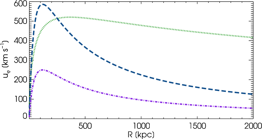
Figure 1: The velocity profiles VP1 (dotted green line), VP2 (dashed blu line) and VP3 (dot-dashed purple line) defined in Section 2.3.

The gas fraction $f_{\rm gas}=M_{\rm ICM}/M_{\rm 200}$, where $M_{\rm ICM}$ is the total mass of the ICM, can be estimated using the observational relation (Eckert et al.,, 2011)

$$f_{\rm gas}(<r_{200})=(0.15\pm 0.01)\left(\frac{k_{\rm B}T}{10\rm\,keV}\right)^{0.478},$$ (14)

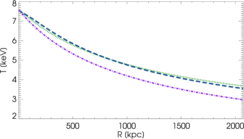
Figure 2: The temperature profiles along $z=0$ for the non-isothermal models NI1 (dotted green line), NI2 (dashed blu line) and NI3 (dot-dashed purple line).

where $T$ is the gas temperature. In the contest of the self-similar model of galaxy clusters, $T$ is expected to be related to the cluster mass by $M_{200}\propto T^{3/2}$. This expectation is confirmed by the observations of massive clusters for which (Arnaud et al.,, 2005)

$$h(z)M_{200}=A_{200}\left(\dfrac{k_{\rm B}T}{5\,\rm keV}\right)^{\alpha},$$ (15)

where $A_{200}\simeq 5.74\times 10^{14}\,M_{\odot}\,$ and $\alpha\simeq 1.49$. For our models with $M_{200}=10^{15}\;M_{\odot}$ at $z=0.1$, through equation (15) we obtain the ICM temperature $T\simeq 8.7\times 10^{7}\;\rm K$ leading (via equation 14) to the gas fraction $f_{\rm gas}\simeq 0.13$, which we adopt for our case study. This value of $f_{\rm gas}$ is in good agreement with Maughan et al., (2008) and Vikhlinin et al. (2006).

We consider two classes of models: isothermal models with polytropic index $\tilde{\gamma}=1$, and non-isothermal models with $\tilde{\gamma}=1.14$ (see Section 2.1), in agreement with the observational constraints by Markevitch et al., (1998) and Vikhlinin et al. (2006). In Section 3 we present results for three rotating isothermal models (I1, I2 and I3) and three rotating non-isothermal models (NI1, NI2 and NI3), characterized by the rotation laws VP1, VP2 and VP3, respectively (see Section 2.3). In all cases we assume that the central temperature is $T_{c}=8.7\times 10^{7}\,K$. When $\Phi$, $f_{gas}$,$\tilde{\gamma}$, $u_{\phi}$ and $T_{c}$ are fixed, the temperature and density distributions can be computed from equation (6), (7), and $T/T_{0}=(\rho/\rho_{0})^{\tilde{\gamma}-1}$. While, by construction, in the isothermal models the temperature is independent of position, in the non-isothermal models the temperature decreases for increasing distance from the centre. The temperature profiles in the $z=0$ plane of the three non-isothermal models are plotted in Fig. 2.

In summary, the parameters common to all models are listed in Table 1, while the specific values of the parameters for each model, including the gas central number density $n_{c}$, are given in Table 2.

3 Observables

We describe here observable quantities of our rotating ICM models to be compared with current or forthcoming observations of real galaxy clusters. We consider X-ray surface brightness maps and X-ray spectra, both of which are affected by rotation. We note that the models here presented are not representative of cool core clusters. We defer the discussion of the effect of cool cores to Section 4.

3.1 X-ray maps and surface brightness profiles

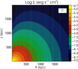
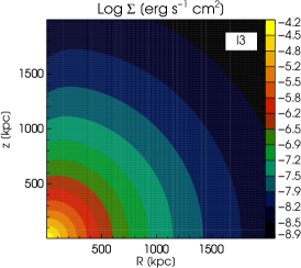
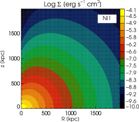
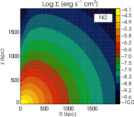
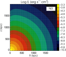
Figure 3: The surface brightness maps of the isothermal (upper panels) and non-isothermal (lower panels) rotating models.

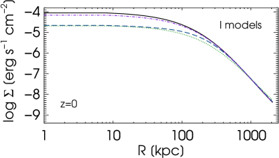
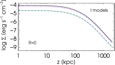
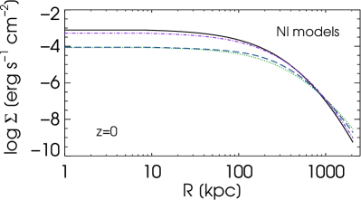
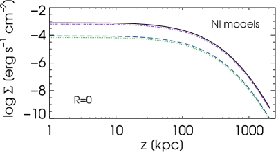
Figure 4: The surface brightness profiles along $z=0$ (left panels) and $R=0$ (right panels), for the isothermal (upper panels) and non-isothermal (lower panels) models. Specifically, the I1 and NI1 (dotted green line), I2 and NI2 (dashed blu line), and I3 and NI3 (dot-dashed purple line) models are shown. The solid lines represent the corresponding non-rotating models.

For each model, the surface brightness map is produced to perform a direct comparison with the observations. The amount of rotational motion directly affects the ICM shape, making the isophotes deviate from circular symmetry. In order to estimate the maximum effect of rotational flattening, we assume that our models are seen edge-on. In this hypothesis, the surface brightness is

$$\Sigma(R,z)=2\int^{\infty}_{R}\dfrac{\dot{E}(R^{\prime},z)R^{\prime}dR^{\prime}}{\sqrt{R^{\prime 2}-R^{2}}},$$ (16)

where $\dot{E}=n_{\rm e}n_{\rm p}\Lambda(T)$ is the gas cooling rate. Here $n_{\rm e}$ and $n_{\rm p}$ are, respectively, the electron and proton number densities, and $\Lambda(T)$ is the cooling function. In particular, we adopt the cooling function by Tozzi & Norman, (2001)

$$\Lambda=C_{1}(k_{\rm B}T)^{\alpha}+C_{2}(k_{\rm B}T)^{\beta}+C_{3},$$ (17)

where the exponents take the values $\alpha={-1.7}$ $\beta=0.5$ and $C_{1}$, $C_{2}$, $C_{3}$ are constants depending on the the ICM metallicity: in all our models we assume a metallicity of $Z=0.3Z_{\odot}$, leading to $C_{1}=8.6\times 10^{-3}\,\rm erg\,cm^{3}\,s^{-1}\,keV^{-\alpha}$, $C_{2}=5.8\times 10^{-2}\,\rm erg\,cm^{3}\,s^{-1}\,keV^{-\beta}$, $C_{3}=6.3\times 10^{-2}\,\rm erg\,cm^{3}\,s^{-1}$.

The resultant ICM morphology of the three rotating isothermal models I1, I2 and I3 and of the non-isothermal models NI1, NI2 and NI3 can be seen in Fig. 3. The effect of the rotation, visible as the flattening of the isophotes, reflects also in the surface brightness profiles along the $z=0$ and $R=0$ axes, shown in Fig. 4. In this figure, for a better comparison, we included the isothermal and non-isothermal non-rotating models, having the same gas fraction and central temperature as the corresponding rotating models. The surface brightness profiles of the rotating models along the axis of rotation ($R=0$) show the depletion of the inner regions, while the surface brightness along $z=0$ is systematically lower than that of the corresponding non-rotating models up to the virial radius.

From the surface-brightness maps shown in Fig. 3 it is apparent that the gas distribution in our models tends to be peanut-shaped, with a depletion of gas along the vertical axis. This effect is particularly strong, because for simplicity we are assuming cylindrical rotation, and we expect it to be mitigated in more realistic baroclinic models in which a vertical gradient in the azimuthal velocity is allowed. In any case, such peanut-shaped distributions would be hardly detectable in observed clusters, in which the decrease of surface brightness in the central regions is interpreted as due to the presence of cavities in the ICM.

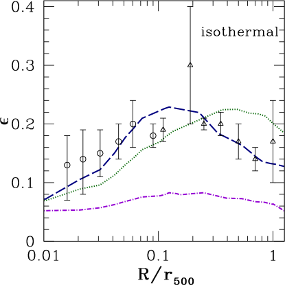
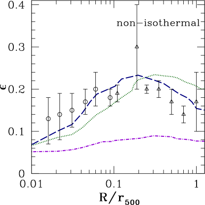
Figure 5: The ellipticity profiles of the isothermal and non-isothermal models (curves) compared with the average ellipticity profile of observed relaxed clusters (points): the circles show the ellipticity estimated using Chandra observations, while the triangles represent the measurements from ROSAT data Lau et al. (2012). The left panel refers to the isothermal models, the right one to the non-isothermal models (I1 and NI1 models: dotted green line; I2 and NI2 models: dashed blue line; I3 and NI3 models: dot-dashed purple line). In all our models $r_{500}\approx 1345\;\rm kpc$.

3.2 X-ray ellipticity profiles

Thanks to the extensive coverage of X-ray surveys of galaxy clusters, the isophote ellipticity can be evaluated for a relatively large sample of observed objects. Fang, Humphrey & Buote (2009) considered 10 relaxed galaxy clusters from the ROSAT PSPC sample of Buote & Tsai (1996), and obtained a Chandra follow up for the central regions ($r\lesssim 100\rm\,kpc$) of the selected clusters. They evaluated an average ellipticity profile with a constant value of $\epsilon\approx 0.25$ up to $\approx 0.7\rm\,r_{500}$. This result is in agreement with Lau et al. (2012), who, using the low-redshift clusters sample from Vikhlinin et al. (2009), showed that the mean observed cluster ellipticity is relatively constant with radius, with $\epsilon\approx 0.18$ in the radial range of $0.05\lesssim r/r_{500}\lesssim 1$. In Fig. 5, we show the ellipticity of our models superimposed to Lau et al. (2012) observations.

We estimate the ellipticity $\epsilon$ of the isophotes in an X-ray map following the same procedure as Lau et al. (2012). Our models are consistent with the observational average ellipticity profile of Lau et al. (2012). In particular, the I2 and NI2 models produce the ellipticity profile with the best agreement with the observations. It is worth noting that the isothermal and non-isothermal models produce similar ellipticity profiles when subjected to the same velocity law. Nonetheless, the non-isothermal models are characterized by slightly higher values of $\epsilon$ in the cluster outskirts. The steeper decrease of the rotation velocity along $R$ for the VP2 models with respect to the VP1 models reflects into the steeper decrease of the ellipticity profiles in the outer regions of the clusters.

3.3 X-ray spectra

Here we discuss the effects of rotation on the X-ray emission lines of the model cluster spectra. The measure of the centroid position of the emission line profile is the most direct way of probing the presence of ICM motions, but so far this method has been mainly limited to theory (Inogamov & Sunyaev, 2003, Rebusco et al., 2008, Zhuravleva et al. 2012) due to the absence of an instrument with a sufficiently high energy resolution. A first measure of the velocity width of cool material in the X-ray luminous cores of a sample of galaxy clusters, galaxy group and elliptical galaxies has been obtained by Sanders & Fabian (2013), who placed limits of the order of $\lesssim 300\,\rm km\,s^{-1}$ by fitting the emission line profiles with a thermal model convolved with a Doppler broadening using the RGS spectrometer on board the XMM telescope.

We build the simulated spectra using our ICM models. Thanks to the high temperature, the emission line spectrum is characterised by the presence of the Fe XXV ($\approx 6.7\;\rm keV$) and Fe XXVI ($\approx 6.9\;\rm keV$) emission lines. Their high emissivity makes them particularly useful for the Doppler shift fitting procedure. We introduce the effect of the gas rotation using the formalism of Inogamov & Sunyaev, (2003). The authors consider that the classical Gaussian shape expected for an emission line can be significantly shifted by large scale coherent gas motion and enlarged by turbulence. Specifically, the Doppler shift can be expressed as

$$\Delta E=6.7(u_{\varphi}/300\;\rm[km\,s^{-1}])\;\rm{eV},$$ (18)

where $u_{\varphi}$ is the ICM large scale velocity. We simulate the observed spectra using the software XSPEC (Arnaud et al.,, 1996). First, we consider the case in which there is no turbulence, through the APEC model. Subsequently, we add a turbulent velocity component, using the BAPEC model.

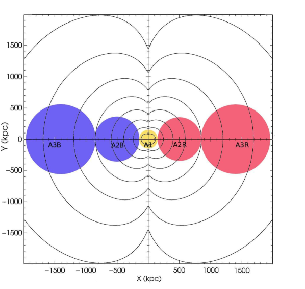
Figure 6: The regions selected for the simulation of the spectra, plotted on the I1 model isophotes. The A1, A2, and A3 label indicate the centre of the inner, intermediate and external region, respectively. We distinguish the blue-shifted (approaching) regions (A2B, A3B) and red-shifted (receding) regions (A2R, A3R).

The cluster is assumed to be observed at redshift $z=0.1$. The data are then convolved in XSPEC with an instrumental response function of the X-ray Calorimeter Spectrometer on board the ASTRO-H satellite, to create the final mock spectra. The convolution with the instrument is performed without considering the background contribution. We recall that the temperature distributions of the models are fixed by choosing $T_{c}\simeq 7.5\rm\;keV$ as central temperature (see Section 2.1). We consider the simulated observations with an exposure time of $300$ ksec and enabling the statistics model included in XSPEC. We select three different circular regions A1, A2 and A3 with radii of $150\;{\rm kpc}\;(1.4$ arcmin at the assumed redshift of 0.1), $350\;{\rm kpc}\;(3.2{\rm\;arcmin})$ and $550\;{\rm kpc}\;(5{\rm\;arcmin})$, respectively, and larger than the spatial extension of about 0.5 arcmin of the single element array of the ASTRO-H Soft X-ray Spectrometer System. Despite the symmetry of our models, we consider separately the blue-shifted (approaching) regions (A2B, A3B) and red-shifted (receding) regions (A2R, A3R) to account for the different response of the instrument at different energies (see Fig. 6).We divide the regions A1, A2 and A3 into 20, 14, and 6 blocks respectively. We assume a constant value of the density for each block, corresponding to its central value. We projected the density onto the sky plane in order to obtain the normalization constant for the models. Then, we evaluate the line-of-sight component of the rotational velocity, being this the factor responsible of the Doppler shift of the emission line centre. In Fig. 7 we show the spectrum of model I1 obtained from the central region (A1): here, the low values of the rotational velocity lead to a broadening of the emission line, and the line centroid position remains unaffected.

For the rotating models, the resulting spectra from region A2 present a shift ranging from $\approx 10\;\rm eV$ for the VP1 model to $\approx 6\;\rm eV$ for the VP2 and $\approx 5\;\rm eV$ VP3 models, in good agreement with Inogamov & Sunyaev, (2003) and with Rebusco et al., (2008). We show the results of the redshift fitting in Table 3 and in Fig. 8, plotted with the respective theoretical emission-weighted shift. Figure 8 shows that it is possible to discriminate between different models, both in the A2 and in the A3 centred observations. It is worth noting that the red-shift and blue-shift results present a slight asymmetry (within the uncertainties) due to the different response of the instrument at different energies. The high central value of the VP2 velocity profile influences globally the fit of models, leading to fit values with the higher discrepancy with respect to the theoretical shift. We can also estimate the amplitude of the detectable velocity constraining it to a lower limit of $\approx 100\;\rm km\,s^{-1}$.

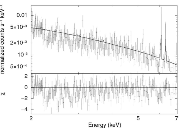
Figure 7: The simulated spectrum of model I1 from the region A1. In the lower plot we show the residuals for the fitting with the APEC spectrum. The Fe XXV and Fe XXVI emission lines are particularly prominent around $E\approx 6\;\rm keV$.

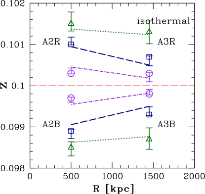
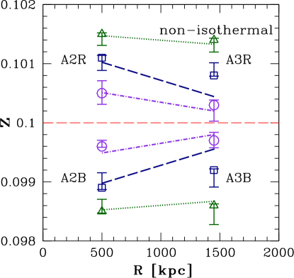
Figure 8: The Doppler shift fitting results for the spectra of models with no turbulence, obtained from the selected areas (A2B, A3B, A2R, A3R) as in Fig 6, plotted as a function of the distance from the cluster centre. The left plot refers to the isothermal models I1 (triangles), I2 (squares) and I3 (circles). The right plot refers to the non-isothermal models NI1 (triangles), NI2 (squares) and NI3 (circles). The corresponding lines refer to the theoretical emission-weighted shift for each model. The horizontal dashed red line indicates the cluster redshift.

The inclusion of the turbulent velocity alters the centroid shift fit. We use the parameters of the APEC models and added a turbulent component $\sigma_{turb}=200\rm\,km\,s^{-1}$ through the BAPEC model included in the XSPEC software. This value is consistent with the current observational limits of $300-500\rm\;km\,s^{-1}$ for the inner regions of bright groups and clusters of galaxies (Sanders & Fabian, 2013). We report the results in Table 3. The Doppler shift fitting suffers from an higher error, but preserves a good significance, in particular for the non-isothermal models. We tested the fitting procedure up to $\sigma_{turb}=600\;\rm km\,^{-1}$, finding that the result remains significant ( $\sigma\approx 1$) up to $\sigma_{turb}=450\;\rm km\,^{-1}$ We can conclude that A2 is the most suitable region for the observation, in which the higher gas density allows to obtain a better fit.

Model	Region	Observed shift	$\rm\sigma_{turb}=200km\;s^{-1}$
		$z_{\rm fit}(2\sigma)$, $\sigma$	$z_{\rm fit}(2\sigma)$, $\sigma$	$\sigma_{turb,fit}$
I1	A2B	$0.0986^{+1.56\times 10^{-4}}_{-3.43\times 10^{-5}}$, $7.3$	$0.0988^{+5.27\times 10^{-4}}_{-5.47\times 10^{-4}}$, $2.1$	$\leq 304.24$
	A2R	$0.1016^{+2.76\times 10^{-5}}_{-1.45\times 10^{-4}}$, $9.2$	$0.1012^{+3.47\times 10^{-4}}_{-3.08\times 10^{-4}}$, $1.8$	$\leq 301.58$
	A3B	$0.0987^{+2.84\times 10^{-4}}_{-2.51\times 10^{-4}}$, $2.6$
	A3R	$0.1013^{+2.12\times 10^{-4}}_{-2.63\times 10^{-4}}$, $2.7$
I2	A2B	$0.0989^{+3.25\times 10^{-5}}_{-1.85\times 10^{-4}}$, $5.0$	$0.0988^{+3.45\times 10^{-4}}_{-4.69\times 10^{-4}}$, $1.4$	$214.25^{+105.7}_{-91.36}$
	A2R	$0.1010^{+1.77\times 10^{-4}}_{-1.24\times 10^{-5}}$, $5.2$	$0.1011^{+1.87\times 10^{-4}}_{-1.98\times 10^{-4}}$, $2.8$	$212^{+104.52}_{-94.57}$
	A3B	$0.0993^{+1.88\times 10^{-5}}_{-2.64\times 10^{-4}}$, $2.5$
	A3R	$0.1007^{+2.14\times 10^{-5}}_{-2.17\times 10^{-4}}$, $2.9$
I3	A2B	$0.0997^{+2.39\times 10^{-5}}_{-1.01\times 10^{-4}}$, $2.5$	$0.0997^{+2.35\times 10^{-4}}_{-1.07\times 10^{-4}}$, $1.0$	$271.25^{+107.21}_{-109.71}$
	A2R	$0.1003^{+1.28\times 10^{-4}}_{-1.3\times 10^{-5}}$, $2.2$	$0.1004^{+2.69\times 10^{-4}}_{-1.25\times 10^{-4}}$, $1.1$	$241.87^{+99.25}_{-112.91}$
	A3B	$0.0998^{+1.09\times 10^{-4}}_{-2.47\times 10^{-5}}$, $1.5$
	A3R	$0.1003^{+2.03\times 10^{-4}}_{-1.41\times 10^{-5}}$ ,$1.3$
NI1	A2B	$0.0985^{+2.24\times 10^{-4}}_{-2.84\times 10^{-5}}$, $5.9$	$0.0986^{+3.02\times 10^{-4}}_{-2.82\times 10^{-4}}$, $2.3$	$207.05^{+92.53}_{-87.58}$
	A2R	$0.1015^{+2.14\times 10^{-5}}_{-1.91\times 10^{-4}}$, $7.1$	$0.1015^{+2.74\times 10^{-}4}_{-3.03\times 10^{-4}},2.5$	$187^{+92.48}_{-87.56}$
	A3B	$0.0986^{+2.78\times 10^{-5}}_{-3.21\times 10^{-4}}$, $4.0$
	A3R	$0.1014^{+3.12\times 10^{-5}}_{-2.03\times 10^{-4}}$, $2.7$
NI2	A2B	$0.0989^{+2.53\times 10^{-4}}_{-2.92\times 10^{-5}}$, $3.8$	$0.0988^{+4.02\times 10^{-4}}_{-2.58\times 10^{-4}}$, $1.8$	$198.72^{+92.37}_{-81.48}$
	A2R	$0.1011^{+3.87\times 10^{-5}}_{-2.15\times 10^{-4}}$, $4.3$	$0.1011^{+4.26\times 10^{-4}}_{-3.25\times 10^{-4}}$, $1.4$	$174^{+94.5}_{-101.84}$
	A3B	$0.0992^{+1.88\times 10^{-5}}_{-2.87\times 10^{-4}}$, $2.6$
	A3R	$0.1008^{+2.15\times 10^{-4}}_{-1.23\times 10^{-5}}$, $3.5$
NI3	A2B	$0.0996^{+1.05\times 10^{-4}}_{-1.48\times 10^{-5}}$, $3.4$	$0.0997^{+1.14\times 10^{-4}}_{-1.35\times 10^{-4}}$, $1.2$	$208.25^{+89.54}_{-92.36}$
	A2R	$0.1005^{+2.11\times 10^{-4}}_{-1.89\times 10^{-5}}$, $2.2$	$0.1005^{+1.38\times 10^{-4}}_{-3.11\times 10^{-4}}$, $1.2$	$175.36^{+71.69}_{-85.36}$
	A3B	$0.0997^{+1.38\times 10^{-4}}_{-1.23\times 10^{-4}}$, $1.2$
	A3R	$0.1003^{+8.65\times 10^{-5}}_{-2.74\times 10^{-4}}$, $2.6$
CC1	A2B	$0.0986^{+2.23\times 10^{-4}}_{-3.11\times 10^{-5}}$, $5.5$	$0.0986^{+4.27\times 10^{-5}}_{-2.89\times 10^{-4}}$, $4.2$	$221.3^{+89.4}_{-73.5}$
	A2R	$0.1014^{+1.98\times 10^{-4}}_{-3.02\times 10^{-5}}$, $6.1$	$0.1013^{+3.25\times 10^{-5}}_{-3.62\times 10^{-4}},3.2$	$198.3^{+86.2}_{-90.2}$
	A3B	$0.0987^{+3.84\times 10^{-4}}_{-2.54\times 10^{-4}}$, $2.1$
	A3R	$0.1013^{+2.01\times 10^{-4}}_{-2.36\times 10^{-4}}$, $2.9$
CC2	A2B	$0.0988^{+2.18\times 10^{-4}}_{-1.35\times 10^{-5}}$, $5.1$	$0.0989^{+1.74\times 10^{-4}}_{-3.98\times 10^{-4}}$, $1.9$	$206.7^{+89.5}_{-92.5}$
	A2R	$0.1012^{+8.57\times 10^{-5}}_{-1.58\times 10^{-4}}$, $5.0$	$0.1008^{+1.56\times 10^{-4}}_{-2.24\times 10^{-4}}$, $2.1$	$196.8^{+102.5}_{-84.9}$
	A3B	$0.0993^{+3.02\times 10^{-4}}_{-2.48\times 10^{-5}}$, $2.2$
	A3R	$0.1005^{+2.11\times 10^{-4}}_{-1.71\times 10^{-5}}$, $2.1$
CC3	A2B	$0.0994^{+1.85\times 10^{-4}}_{-2.71\times 10^{-5}}$, $2.8$	$0.0994^{+3.89\times 10^{-4}}_{-1.18\times 10^{-4}}$, $1.2$	$215.9^{+98.1}_{-105.8}$
	A2R	$0.1004^{+3.15\times 10^{-5}}_{-1.54\times 10^{-4}}$, $2.2$	$0.1004^{+1.54\times 10^{-4}}_{-2.89\times 10^{-4}}$, $1.1$	$199.8^{+102.5}_{-95.4}$
	A3B	$0.0997^{+3.55\times 10^{-5}}_{-1.12\times 10^{-4}}$, $2.0$
	A3R	$0.1003^{+2.84\times 10^{-5}}_{-1.25\times 10^{-4}}$, $1.9$

Table 3: Spectral constraints on the rotating ICM. From left to right, we have the model name (column 1), the region considered (column 2), the result of the Doppler shift fitting of the rotating models and its significance (column 3), and the Doppler shift fitting of the rotating models with a turbulent component and its significance (column 4). We recall that when computing the mock spectra we assume that the clusters are at redshift $z=0.1$.

4 Effect of cool cores

So far we have considered models of non-cool core clusters. In this section, we discuss the effect of cool cores on the ICM properties investigated in our study. Here we limit ourselves to presenting toy models of rotating clusters with cool cores, assuming that these systems are stationary, and so neglecting the complex interplay of cooling and heating in the central regions. In this spirit, we assume that these rotating cool-core (CC) models have the same temperature profiles in the outer regions as the NI models, but we impose an outward increasing temperture profile in the core. To reproduce this behaviour, we use composite polytropes, assuming the following relation between pressure and density:

$$\dfrac{P}{P_{0}}=\left(\dfrac{\rho}{\rho_{0}}\right)^{\tilde{\gamma}_{in}}\rm\;\;\;\ if\;\rho>\rho_{0},$$ (19)

$$\dfrac{P}{P_{0}}=\left(\dfrac{\rho}{\rho_{0}}\right)^{\tilde{\gamma}_{out}}\rm\;\;\;\ if\;\rho<\rho_{0},$$ (20)

where $\rho_{0}$ and $P_{0}$ are the gas density and pressure at the boundary between the inner (core) region and the outer region, and we assume $\tilde{\gamma}_{in}=0.59$ and $\tilde{\gamma}_{out}=1.14$. We present here three CC models, named CC1, CC2, CC3, having respectively velocity profiles VP1, VP2, VP3. The global properties of these models are the same as for models I and NI (see Table 1). In terms of the gas number density $n_{0}$ and temperature $T_{0}$ at the boundary (related to pressure and density by $P_{0}=n_{0}k_{B}T_{0}$ and $\rho_{0}=\mu m_{p}n_{0}$, where $\mu=0.59$ and $m_{p}$ is the proton mass), we assume $n_{0}=5.37\,\rm\times 10^{-3}\,cm^{-3}$ , $k_{B}T_{0}=6.9\,\rm keV$ for model CC1, $n_{0}=6.31\,\rm\times 10^{-3}cm^{-3}$ , $k_{B}T_{0}=7.1\,\rm keV$ for model CC2, and $n_{0}=11.48\,\times 10^{-3}\rm cm^{-3}$, $k_{B}T_{0}=6.79\,\rm keV$ for model CC3. In Fig. 9 we plot the temperature profiles in the $z=0$ plane, for the rotating CC models.

We obtain the surface brightness profiles along the $z=0$ and $R=0$ axes, shown in Fig. 10, where we included the composite non-rotating model, having the same gas fraction as the corresponding rotating models. The surface brightness profiles of the rotating models along $R=0$ and $z=0$ present a depletion of the inner regions comparable to the I and NI models. As expected, the CC models have higher central surface brightness compared to the NI models and steeper inner surface brightness profiles. The ellipticity profiles of the CC models are shown in Fig 11: the profiles are similar to those of the I and NI models, and therefore consistent with the observations by Lau et al. (2012).

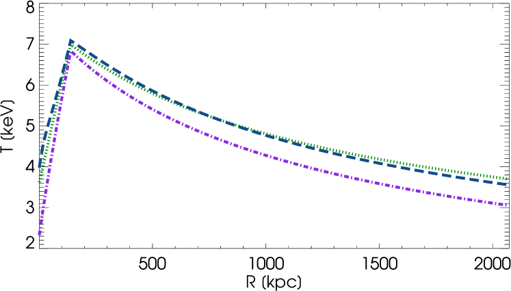
Figure 9: The temperature profiles along $z=0$ for the CC models CC1 (dotted green line), CC2 (dashed blu line) and CC3 (dot-dashed purple line).

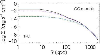
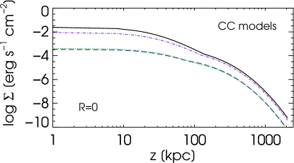
Figure 10: The surface brightness profile along $z=0$ (left panel) and $R=0$ (right panel), for the cool core models. Specifically, the CC1 (dotted green line), CC2 (dashed blu line), and CC3 (dot-dashed purple line) models are shown. The solid lines represent the corresponding non-rotating model

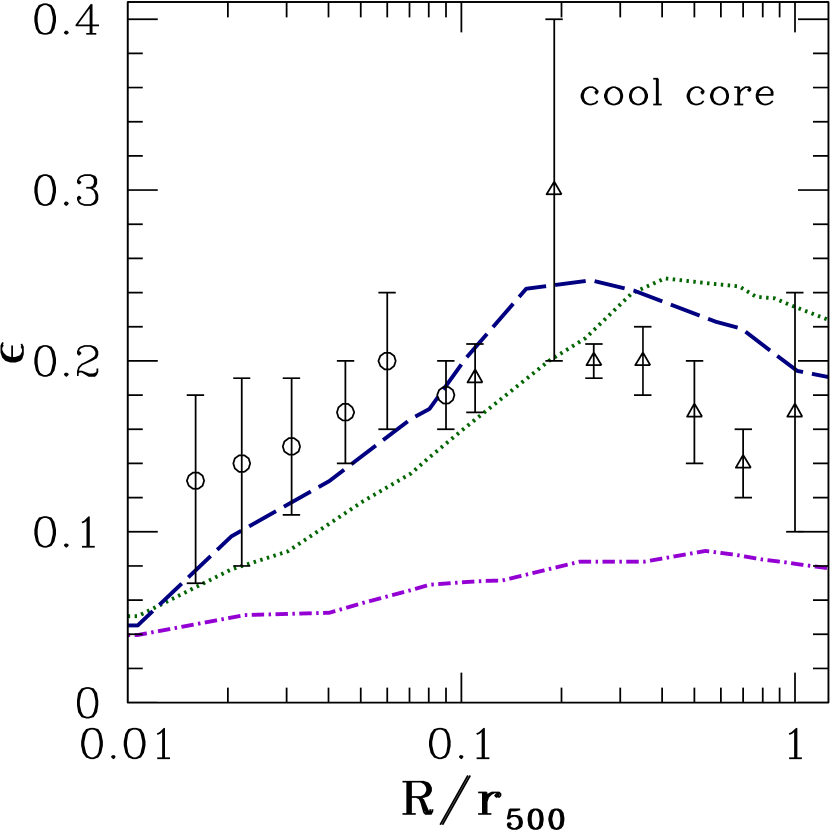
Figure 11: The ellipticity profiles of our CC models (curves). The different line types represent the cool core models as in Fig. 9. The symbols with error bars are the same as in Fig. 5.

Following the procedure in Section 3.3, we build the simulated spectra of the CC models. The resulting spectra from region A2 present a shift ranging from $\approx 11\;\rm eV$ for the VP1 model to $\approx 6\;\rm eV$ for the VP2 and $\approx 5\;\rm eV$ VP3 models, similar to the values obtained for the non-cool core models (see Section 3.3). We show the results of the redshift fitting in Table 3 and in Fig. 12, plotted with the corresponding theoretical emission-weighted shift. We note again a slight asymmetry (within the uncertainties) due to the different response of the instrument at different energies. Globally, the CC models maintain the same properties as the I and NI models.

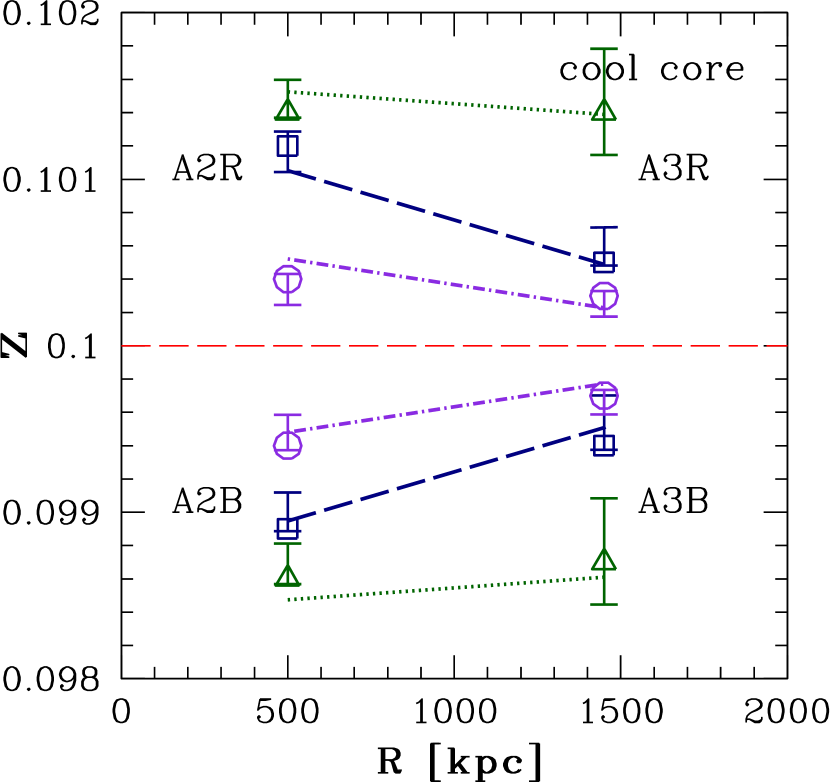
Figure 12: Same as Fig. 8, but for the cool core models CC1 (triangles), CC2 (squares) and CC3 (circles).

5 Conclusion

The study of the dynamics of the intracluster medium is fundamental to depict the physical processes involved in the cluster evolution. In this work, we demonstrate the capability of the X-ray observations to characterise the features induced from a rotating ICM on the shape of the surface brightness isophotes and on the spectral emission lines. This can be extended to test the hydrostatic equilibrium hypothesis on which the majority of the current X-ray mass estimate and calibrations of the scaling laws relies. We consider, as case study, representative models of massive galaxy clusters with a spherical dark matter halo. A simple modelling of the gas, obtained through the assumption of a polytropic distribution $P\propto\rho^{\tilde{\gamma}}$, allow us to span the whole range of the observed ellipticity profiles and to reproduce the observed values of Lau et al. (2012). For instance, we find good agreement with the observed ellipticities for the rotation profile VP2, with a peak velocity of $\approx 600\rm\;km\,s^{-1}$ at $0.05\;\rm r_{200}$ decreasing to $\approx 130\rm\;km\,s^{-1}$ at $\rm r_{200}$. We demonstrate also the capability of the future generation of the X-ray calorimeter expected to fly onboard the next generation of X-ray satellites, like the X-ray Calorimeter Spectrometer onboard the ASTRO-H, to investigate some of the features induced by rotating ICM. Thanks to its excellent energy resolution (with a goal of $\Delta E\approx 4\;\rm eV$), such a calorimeter is suitable for detecting the Doppler shift ($\Delta E\approx 10\;\rm eV$, $\Delta E\approx 6\;\rm eV$ and $\Delta E\approx 5\;\rm eV$ for our VP1, VP2 and VP3 models, respectively) and the emission line broadening (of the order of $\approx 100\rm\,km\;s^{-1}$) on the ICM emission lines with a good significance. Together with a resolved imaging of the ICM isophotes and the determination of their ellipticity, a calorimeter-like detector will permit to discriminate among the different velocity profiles here considered. We have extended this procedure to cool-core clusters, by using composite polytropic profiles. Overall, the cool-core models are similar, in terms of ellipticity profile and spectral line shift, to the corresponding non cool-core models. A natural extension of our work would be the introduction of less crude rotation velocity patterns, for instance considering baroclinic distributions, in which the azimuthal velocity is not stratified on cylinders. This would help in obtaining a more regular gas morphology. Also the question of the thermal stability of these rotating models has to be addressed in detail. Finally, it would be useful to compare the ICM shape obtained with high-resolution SZ imaging. This is a potentially powerful means of extending this analysis to higher redshifts, because of the redshift independence of the SZ effect.

References

- Arnaud et al., (1996) Arnaud K. A., 1996, in G. H. Jacoby & J. Barnes ed., Astronomical Data Analysis Software and Systems V Vol. 101 of Astronomical Society of the Pacific Conference Series, XSPEC: The First Ten Years. p. 17
- Arnaud et al., (2005) Arnaud M., Pointecouteau E., Pratt G. W., 2005, A&A, 441, 893
- Balbus & Reynolds (2010) Balbus S. A., Reynolds C. S., 2010, ApJ, 720, L97
- Biffi, Dolag & Böhringer (2011,2013) Biffi V., Dolag K., Böhringer H., 2011, MNRAS, 413, 573
- Biffi, Dolag & Böhringer (2013) Biffi V., Dolag K., Böhringer H., 2013, MNRAS, 428, 1395
- Brighenti & Mathews (1996) Brighenti F., Mathews W. G., 1996, ApJ, 470, 747
- Buote & Tsai (1996) Buote D. A., Tsai J. C., 1996, ApJ, 458, 27
- Buote & Canizares (1996) Buote D. A., Canizares C. R., 1996, ApJ, 457, 565
- Buote & Humphrey (2012ab) Buote D. A., Humphrey P. J., 2012a, MNRAS, 420, 1693
- Buote & Humphrey b (2012) Buote D. A., Humphrey P. J., 2012b, MNRAS, 421, 1399
- Dolag et al, (2004) Dolag K., Bartelmann M., Perrotta F., Baccigalupi C., Moscardini L., Meneghetti M., Tormen G., 2004, A&A, 416, 853
- Eckert et al., (2011) Eckert D., Vazza F., Ettori S., Molendi S., Nagai D., Lau E. T., Roncarelli M., Rossetti M., Snowden S.L., Gastaldello F., 2012, A&A, 541, 57
- Ettori et al., (2010) Ettori S., Gastaldello F., Leccardi A., Molendi S., Rossetti M., Buote D., Meneghetti M., 2010, A&A, 524, A68
- Fang, Humphrey & Buote (2009) Fang T., Humphrey P., Buote D., 2009, ApJ, 691, 1648
- Humphrey et al. (2012) Humphrey P. J., Buote D. A., Brighenti F., Gebhardt K., Mathews W. G., 2012, arXiv, arXiv:1205.0256
- Jing & Suto (2002) Jing Y. P., Suto Y., 2002, ApJ, 574, 538
- Kawahara (2010) Kawahara H., 2010, ApJ, 719, 1926
- Kravtsov & Borgani (2012) Kravtsov A., Borgani S., 2012, arXiv, arXiv:1205.5556
- Inogamov & Sunyaev, (2003) Inogamov N. A., Sunyaev R. A., 2003, Astronomy Letters, 29, 791
- Lau, Kravtsov, & Nagai (2009) Lau E. T., Kravtsov A. V., Nagai D., 2009, ApJ, 705, 1129
- Lau et al. (2012) Lau E. T., Nagai D., Kravtsov A. V., Vikhlinin A., Zentner A. R., 2012, ApJ, 755, 116
- Mahdavi et al. (2008) Mahdavi A., Hoekstra H., Babul A., Henry J. P., 2008, MNRAS, 384, 1567
- Malagoli, Rosner, & Bodo (1987) Malagoli A., Rosner R., Bodo G., 1987, ApJ, 319, 632
- Markevitch et al., (1998) Markevitch M., Forman W. R., Sarazin C. L., Vikhlinin A., 1998, ApJ, 503, 77
- Mathews & Bregman (1978) Mathews W. G., Bregman J. N., 1978, ApJ, 224, 308
- Maughan et al., (2008) Maughan B. J., Jones C., Forman W., Van Speybroeck L., 2008, ApJS, 174, 117
- Meneghetti et al. (2010) Meneghetti M., Rasia E., Merten J., Bellagamba F., Ettori S., Mazzotta P., Dolag K., Marri S., 2010, A&A, 514, A93
- Morandi, Pedersen, & Limousin (2010) Morandi A., Pedersen K., Limousin M., 2010, ApJ, 713, 491
- Morandi, Nagai, & Cui (2012) Morandi A., Nagai D., Cui W., 2012, arXiv, arXiv:1211.7096
- Nagai, Vikhlinin, & Kravtsov (2007) Nagai D., Vikhlinin A., Kravtsov A. V., 2007, ApJ, 655, 98
- Navarro, Frenk & White (1996) Navarro J. F., Frenk C. S., White S. D. M., 1996, ApJ, 462, 563
- Nipoti (2010) Nipoti C., 2010, MNRAS, 406, 247
- Nipoti & Posti (2013) Nipoti C., Posti L., 2013, MNRAS, 428, 815
- Roediger et al. (2012) Roediger E., Lovisari L., Dupke R., Ghizzardi S., Brüggen M., Kraft R. P., Machacek M. E., 2012, MNRAS, 420, 3632
- Rasia, Tormen, & Moscardini (2004) Rasia E., Tormen G., Moscardini L., 2004, MNRAS, 351, 237
- Rasia et al. (2006) Rasia E., et al., 2006, MNRAS, 369, 2013
- Rasia et al. (2012) Rasia E., et al., 2012, NJPh, 14, 055018
- Rebusco et al., (2008) Rebusco P., Churazov E., Sunyaev R., Böhringer H., Forman W., 2008, MNRAS, 384, 1511
- Sanders & Fabian (2013) Sanders J. S., Fabian A. C., 2013, MNRAS, 429, 2727
- Sereno et al. (2013) Sereno M., Ettori S., Umetsu K., Baldi A., 2013, MNRAS, 428, 2241.
- Smith et al. (2005) Smith G. P., Kneib J.-P., Smail I., Mazzotta P., Ebeling H., Czoske O., 2005, MNRAS, 359, 417
- Sunyaev & Zeldovich (1970) Sunyaev R. A., Zeldovich Y. B., 1970, Ap&SS, 7, 3
- Suto et al. (2013) Suto D., Kawahara H., Kitayama T., Sasaki S., Suto Y., Cen R., 2013, ApJ in press (arXiv:1302.5172)
- Takahashi et al. (2010) Takahashi T., et al., 2010, SPIE, 7732,
- Tassoul, (1978) Tassoul J.-L., 1978, Theory of rotating stars (Princeton: Princeton University Press)
- Tozzi & Norman, (2001) Tozzi P., Norman C., 2001, ApJ, 546, 63
- Valdarnini (2011) Valdarnini R., 2011, A&A, 526, A158
- Vikhlinin et al. (2006) Vikhlinin A., Kravtsov A., Forman W., Jones C., Markevitch M., Murray S. S., Van Speybroeck L., 2006, ApJ, 640, 691
- Vikhlinin et al. (2009) Vikhlinin A., et al., 2009, ApJ, 692, 1033
- Voit (2005) Voit G. M., 2005, RvMP, 77, 207
- Zhang et al. (2008) Zhang Y.-Y., Finoguenov A., Böhringer H., Kneib J.-P., Smith G. P., Kneissl R., Okabe N., Dahle H., 2008, A&A, 482, 451
- Zhuravleva et al. (2012) Zhuravleva I., Churazov E., Kravtsov A., Sunyaev R., 2012, MNRAS, 422, 2712