Coherent dynamics of Rydberg atoms in cosmic microwave background radiation

Abstract

Rydberg atoms excited by cold blackbody radiation are shown to display long-lived quantum coherences on timescales of tens of picoseconds. By solving non-Markovian equations of motion with no free parameters we obtain the time evolution of the density matrix, and demonstrate that the blackbody-induced temporal coherences manifest as slowly decaying (100 ps) quantum beats in time-resolved fluorescence. An analytic model shows the dependence of the coherent dynamics on the energy splitting between atomic eigenstates, transition dipole moments, and coherence time of the radiation. Experimental detection of the fluorescence signal from a trapped ensemble of $10^{8}$ Rydberg atom is discussed, but shown to be technically challenging at present, requiring CMB amplification somewhat beyond current practice.

I introduction

The interactions of atoms and molecules with incoherent light (such as blackbody radiation, BBR) play a central role in research fields as diverse as photosynthesis Fleming ; Scholes ; ScholesJPCL ; PNAS , photovoltaics Scully , precision spectroscopy and measurement BBRshifts , and atomic and molecular cooling and trapping RA ; Bas . Thermal BBR is a ubiquitous perturber that shifts atomic energy levels FarleyWing , limiting the accuracy of modern atomic clocks BBRshifts ; Gibble , and reducing the lifetime of Rydberg atoms RA ; Kleppner82 ; 6K ; Tada and trapped polar molecules Bas . Recent theoretical developments suggest, however, that quantum noise-induced coherence effects induced by BBR can be used to cool quantum systems Cooling and enhance the efficiency of solar cells Scully .

The dynamical response of a material system to incoherent light is determined, among other factors, by the coherence time, a timescale over which the phase relationship between the different frequency components of the light source is maintained Loudon . A natural light source such as the Sun is well characterized as a black body radiation (BBR) emitter with temperature $T=5.6\times 10^{3}$ K, and extremely short coherence time of $\tau_{c}=\hbar/kT\sim 1.3$ fs MehtaWolf ; KanoWolf ; Zaheen ; Hoki ; Leonardo , where $k$ is the Boltzmann constant. As a consequence, incoherent excitation of atomic systems on timescales relatively long compared to $\tau_{c}$ produces stationary mixtures of atomic eigenstates that do not evolve in time PNAS ; JB ; Hoki ; Leonardo . However, the coherence time of BBR increases with decreasing temperature and can reach values in excess of 2 ps at 2.7 K, the temperature of the cosmic microwave background radiation (CMB) CMBbook . This motivates interest in examining the temporal dynamics of atomic systems interacting with the CMB. However, since the CMB intensity is $(300/2.7)^{4}$ = $1.5\times 10^{8}$ weaker than that of BBR at 300 K, the absorption signal in most ground-state atoms and molecules even with suitably amplified CMB radiation Amplifiers , is very small. As an initial step toward resolution of this difficulty, we propose to use highly excited Rydberg atoms, whose large transition dipole moments make them extremely sensitive to external field perturbations RA . Previous experimental work has explored the absorption of BBR by Rydberg atoms, leading to population redistribution, photoionization, and lifetime shortening RA ; Kleppner82 ; 6K . However, these experiments were focused on measuring population dynamics with no attention to coherence effects. Similarly, no attention has been paid to coherence properties of CMB and the role it might play in enhancing cosmological information (e.g. Weinberg ; Hinshaw ; Amanullah ; Hakim ).

In this Article we examine long-lived quantum coherence effects that occur in one-photon absorption of cold black body radiation (CBBR – a term that we henceforth use to denote BBR at 2.7 K) by highly excited Rydberg atoms RA . Using a non-Markovian approach JB ; TBP to explore the dynamics of one-photon CBBR absorption, we show that the time-dependent fluorescence intensities of Rydberg atoms exhibit the quantum beats due to the coherences induced by a suddenly turned-on interaction with CBBR. This suggests an experiment to explore the coherence properties of a cold trapped ensemble of Rb atoms in the presence of CBBR. Our results demonstrate that non-Markovian and quantum coherence effects play a major role in short-time population dynamics induced by CBBR.

Furthermore, we develop an analytical model for the coherences in the long-time limit that is valid for an arbitrary noise source, here applied to CBBR. The model reproduces the coherent oscillations observed in numerical simulations of the density matrix, and provides insight into the role of the energy level splittings, transition dipole moments, and the coherence time of the radiation in determining the time evolution of the coherences. Significantly, we show that the ratio of coherences to populations declines with time as 1/$|\omega_{ij}t|$, where $\omega_{ij}$ is the energy splitting between the eigenstates $i$ and $j$. Thus, the physical origin of the long-lived coherences is due to the small energy splittings between the eigenstates populated by one-photon absorption of CBBR.

The paper is organized as follows. Section II discusses the theory and Section III provides results and a discussion of the nature of the development and depletion of the coherences.

II Theory

Theoretically, the interaction of blackbody radiation with atoms is usually considered within the framework of Markovian quantum optical master equations BPbook , leading to Pauli-type rate equations for state populations parametrized by the Einstein coefficients. These treatments generally assume that the coherences induced by BBR are negligibly small. The non-Markovian approach adopted here JB ; TBP ; Leonardo allows us to examine these noise-induced coherences and memory effects arising from a finite correlation time of BBR.

The time evolution of atomic populations and coherences under the influence of incoherent radiation (such as BBR), suddenly turned on at $t=0$, is given by Zaheen ; JB ; TBP

$$\rho_{ij}(t)=\frac{\langle\mu_{i0}\mu_{j0}^{*}\rangle_{p}}{\hbar^{2}}e^{-\text{i}\omega_{ij}t}\\ \times\int_{0}^{t}d\tau^{\prime}\int_{0}^{t}d\tau^{\prime\prime}\mathcal{C}(\tau^{\prime},\tau^{\prime\prime})e^{\text{i}\omega_{i0}\tau^{\prime}}e^{-\text{i}\omega_{j0}\tau^{\prime\prime}}$$ (1)

Here $\rho_{ij}(t)$ are the elements of the atom density matrix in the energy representation, $\mu_{i0}=\langle 0|\hat{\mu}|i\rangle$ are the transition dipole moment matrix elements connecting the initial atomic eigenstate $|0\rangle=|n_{0}l_{0}m_{0}\rangle$ and the final states $|i\rangle=|nlm\rangle$ with energies $\epsilon_{0}$ and $\epsilon_{i}$, $\langle...\rangle_{p}$ denotes polarization-propagation average Griffiths , and $\omega_{ij}=(\epsilon_{i}-\epsilon_{j})/\hbar$. For the sake of clarity, we further assume that the atom resides in a single state $|0\rangle=|n_{0}l_{0}m_{0}\rangle$ before the BBR is turned on at $t=0$. Since $\rho_{00}\simeq 1$ at all times, the density matrix [Eq. (1)] describes the populations and coherences among the states populated by BBR excluding the initial state JB .

The dynamics of the atom’s response to incoherent radiation is determined by the two-time electric field correlation function $\mathcal{C}(\tau^{\prime},\tau^{\prime\prime})=\langle\mathcal{E}(\tau^{\prime})\mathcal{E}^{*}(\tau^{\prime\prime})\rangle$ in Eq. (1). For a stationary BBR source, the correlation function depends only on $\tau=\tau^{\prime}-\tau^{\prime\prime}$, and is given by MehtaWolf ; KanoWolf

$$\mathcal{C}(\tau)=\mathcal{E}_{0}^{2}({90}/{\pi^{4}})\zeta(4,1+\text{i}\lambda\tau)$$ (2)

where $\zeta(4,x)$ is the generalized Riemann zeta-function MehtaWolf ; KanoWolf , $\lambda=kT/\hbar$, $T$ is the temperature of the BBR, and $\mathcal{E}_{0}^{2}=[2\pi^{3}/(45\hbar^{3}c^{3})](kT)^{4}$ is the mean intensity of the BBR electric field Itano ; MehtaWolf ; KanoWolf . Note that Eq. (2) applies when $\omega_{i0}>0$ (absorption); $\mathcal{C}^{*}(\tau)$ should be used for stimulated emission ($\omega_{i0}<0$). Because $\langle\mathcal{E}(\tau^{\prime})\mathcal{E}(\tau^{\prime\prime})\rangle=0$ for CBBR Loudon ; BPbook , there is no coherence between those levels populated in absorption and those levels populated in stimulated emission from a given initial state TBP . Combining Eq. (2) with Eq. (1), and evaluating the time integrals, gives (see Appendix A for details)

$$\rho_{ii}(t)=\frac{\langle|\mu_{i0}|^{2}\rangle_{p}}{\hbar^{2}}\biggl{(} t[\mathcal{K}_{0}^{(+)}(\omega_{i0},t)+\mathcal{K}_{0}^{(-)}(\omega_{i0},t)]$$

$$\,\,\,\,-\mathcal{K}_{1}^{(+)}(\omega_{i0},t)-\mathcal{K}_{1}^{(-)}(\omega_{i0},t)\biggr{)}$$ (3)

where

$$\mathcal{K}_{n}^{(\pm)}(\omega,t)=\int_{0}^{t}\tau^{n}\mathcal{C}(\pm\tau)e^{\pm\text{i}\omega\tau}d\tau$$ (4)

are half-Fourier transforms of $\tau$-scaled time correlation functions. In the long-time limit ($t\to\infty$), the right-hand side of Eq. (II) grows linearly with $t$. Note that since we neglect spontaneous emission, the long-time limit is restricted to timescales short compared to the (very long) radiative lifetime, 200 $\mu$s, of the $65s$ state BeterovPRA . Using an integral representation for the generalized Riemann zeta function, we obtain the limit (See Appendix A for details)

$$\rho_{ii}(t)=\frac{2\pi}{\hbar^{2}}\langle|\mu_{i0}|^{2}\rangle_{p}I(\omega_{i0})t\quad(t\to\infty),$$ (5)

where $I(\omega)=\frac{2\hbar^{3}}{\pi c^{3}}\frac{\omega^{3}}{e^{\hbar\omega/kT}-1}$ is proportional to Planck’s spectral density of BBR Loudon . Hence, in the long-time (Markovian) limit, this approach reduces to Fermi’s Golden Rule Griffiths commonly used to calculate the rates of BBR-induced population transfer RA ; BeterovPRA .

The off-diagonal elements of the density matrix are obtained in Appendix A as

$$\rho_{ij}(t) =\frac{\langle\mu_{i0}\mu_{j0}^{*}\rangle_{p}}{\hbar^{2}}\frac{1}{\text{i}\omega_{ij}}\biggl{(}[\mathcal{K}_{0}^{(+)}(\omega_{j0},t)+\mathcal{K}_{0}^{(-)}(\omega_{i0},t)]$$

$$\,\,\,\,-e^{-\text{i}\omega_{ij}t}[\mathcal{K}_{0}^{(+)}(\omega_{i0},t)+\mathcal{K}_{0}^{(-)}(\omega_{j0},t)]\biggr{)}$$ (6)

Note that due to the double half-Fourier transforms in Eq. (1), Eq. (II) is sensitive to frequency cross correlations in the CBBR.

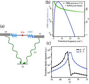
Fig. 1: (a) Proposed experimental setup for observing long-lived quantum coherences with Rydberg atoms. At time $t=0$, the atom in the $65p$ Rydberg state (red circle) begins to interact with CBBR (wavy lines), leading to a decohering Rydberg wavepacket composed of the $ns$ and $nd$ states. The wavepacket evolves and decays to the $5p$ state, with the quantum coherences leaving their signatures in the fluorescence signal $I(t)$ (see text). (b) Binding energies of highly excited $ns$ Rydberg states of ⁸⁵Rb together with the 2.7 K Planck spectrum of CBBR radiation. The zero of energy corresponds to the ionization threshold. (c) $n$ dependence of the calculated transition dipole moments squared from the initial $65p$ state to the $ns$ states (triangles) and $nd$ states (circles)

III Results and Discussion

III.1 Quantum dynamics of Rydberg atoms in CBBR: Populations and Coherences

We now apply the approach developed in Sec. II to examine the effects of quantum coherence in CBBR excitation of high$-n$ Rydberg atoms. In order to parametrize the equations of motion (1), the Rydberg energies and transition dipole moments for ⁸⁵Rb are calculated by solving the radial Schrödinger equation for the Rydberg electron using the Numerov method RA ; Zimmerman ; TBP . To verify the accuracy of our results, we calculated the spontaneous emission rates from the $30s$ Rydberg state to various final $np$ states. These results agree with those reported in BeterovPRA to within $<5\%$.

Figure 1(a) shows the proposed setup for examining CBBR-induced coherences. A highly excited Rydberg state of an alkali-metal atom (here we focus on the $65p$ state of ⁸⁵Rb) is created at $t=0$ by e.g., excitation from the ground $5s$ state RydbergWP . The newly prepared Rydberg state immediately starts to interact with the 2.7 K CBBR background, establishing a coherent superposition of the neighboring $ns$ and $nd$ Rydberg states Kleppner82 . In order to map out the time evolution of Rydberg populations and coherences, Eq. (1) is parametrized by the accurate transition dipole moments of ⁸⁵Rb and by the CBBR correlation function given by Eq. (2).

The rapid turn-on of CBBR acts as a coherent perturbation, creating a Rydberg wavepacket that evolves with time, and then slowly decoheres. Figure 1(b) shows the Rydberg energy levels of ⁸⁵Rb superimposed on the CBBR spectrum at 2.7 K. While the spectral width of the radiation is broad enough to excite the Rydberg levels with principal quantum numbers $n=35-115$, the transition dipole moments (Fig. 1c) decrease dramatically with increasing $\Delta n=n-n_{0}$, so most of the population transfer from the $65p$ state occurs to the neighboring Rydberg states with the largest transition dipole moments (see Fig. 1c) via one-photon absorption ($66s,\,64d$) and stimulated emission ($65s,\,63d$). For this reason, CBBR-induced photoionization occurs at a slow rate and can be neglected for $n_{0}=65$. Spontaneous emission from the $65p$ state is also neglected since it occurs on a much longer timescale (200 $\mu$s BeterovPRA ) than considered in this work.

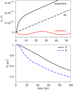
Fig. 2: (a) The population of the representative $65s$ state of Rb as a function of time; (b) The time dependence of the purities for the absorption and stimulated emission blocks of the density matrix (7). The dashed line in the upper panel shows the expected Markovian behavior of the populations.

Figure 2(a) shows the time evolution of several representative density matrix elements given by Eqs. (II) and (II). At $t\leq$ 50 ps, the off-diagonal elements of the density matrix are of the same order of magnitude as the diagonal elements, suggesting the presence of coherences that play a role in the dynamical evolution of a Rydberg atom during the first 50 ps of its exposure to CBBR. At short times, state populations exhibit substantial deviations from the linear behavior predicted based on the standard Markovian quantum optical master equation BPbook . The latter is shown in Fig. 2(a) as the linear solution $\rho_{ii}(t)=W_{0\to i}t$, where $W_{0\to i}$ is the standard BBR-induced transition rate related to the Einstein $B$-coefficient RA . The exact non-Markovian population dynamics is different in character and magnitude TBP but becomes linear in the larger $t$ limit.

As shown in Fig. 2(a), the diagonal elements of the density matrix grow linearly with time while off-diagonal elements oscillate. As a result, the populations begin to significantly dominate over the coherences. Thus, BBR excitation produces a stationary mixture of atomic eigenstates, with coherences playing a negligible role in the long-time limit (nanoseconds) Leonardo ; Zaheen . This gradual reduction of the coherences to population ratio is the mechanism of BBR-induced decoherence for the particular initial state. It differs from other cases Elran1 ; Elran2 where the initial state is a coherent superposition of energy eigenstates.

To see the decoherence times more clearly, Fig. 2(b) shows a useful measure of decoherence—the purity of the density matrix Schlosshauer

$$\varsigma=\text{Tr}\left(\rho_{\pm}^{2}\right)=[N_{\pm}(t)]^{-1}\sum_{i,j=1}|\langle i|\rho_{\pm}(t)|j\rangle|^{2}$$ (7)

where $\rho_{\pm}$ are the subblocks of the full density matrix composed of the states populated in absorption and stimulated emission from the initial state and the normalization factors $N_{\pm}(t)=\sum_{i}\langle i|\rho_{\pm}(t)|i\rangle^{2}$ ensure trace conservation TG . The purity decays over a time scale $>$100 ps, which signals the formation of an incoherent statistical mixture of atomic eigenstates in the process of CBBR excitation.

As is typical of direct CBBR measurements, the populations in Fig. 2(a) are quite small. As such, we note standard CMB amplification practices Amplifiers , which at present can give power gains in excess of 65 dB. Below we report results for a gain of 90 dB, which is technically possible, but experimentally challenging.

III.2 Observables: Time-resolved Fluorescence

While clearly suggesting the existence of long-lived coherences on timescales of up to $\sim$100 ps, neither the density matrix elements nor the purity plotted in Fig. 2 are experimental observables. To explore the possibility of experimentally measuring the long-lived Rydberg coherences, we evaluate the time-resolved fluorescence signal from the $ns$ and $nd$ states of ⁸⁵Rb populated by the interaction with CBBR (see Fig. 1). These states decay to the $5p$ state of Rb ($|i_{f}\rangle$) by emitting a photon at a transition frequency of 620 nm, which can be detected with high quantum efficiency. The total power emitted on these transitions by $N_{a}$ atoms is given by Demtroder ; JB

$$I(t)=I_{0}\text{Tr}\left\{|\hat{\mu}i_{f}\rangle\langle i_{f}\hat{\mu}|\rho(t)\right\}=I_{0}\sum_{i,j=1}\mu_{ii_{f}}\mu_{i_{f}j}\rho_{ji}(t)$$ (8)

where $I_{0}=N_{a}\frac{4}{3}\omega^{4}/(4\pi\epsilon_{0}c^{3})$, $\epsilon_{0}$ is the vacuum permittivity, $c$ is the speed of light, and $\omega$ is the transition frequency, assumed the same for all $i,j$ states (since $|\omega_{ij}|\ll|\omega_{ii_{f}}|$).

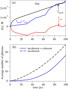
Fig. 3: (a) Time-dependent fluorescence intensity for $N_{a}=10^{8}$ Rydberg atoms initially in the $n_{0}=65p$ state interacting with CBBR amplified by a factor of 90 dB. (b) Average number of emitted photons $N_{\text{ph}}(t)$ (see text). The final state to which fluorescence occurs is $|i_{f}\rangle=|5p\rangle$. Also shown are the incoherent and coherent contributions to the total fluorescence intensity and to $N_{\text{ph}}(t)$.

Figure 3(a) shows the calculated time dependence of the fluorescence intensity for $N_{a}=10^{8}$ Rb atoms interacting with amplified CBBR. The time-resolved emission signal displays pronounced oscillations over the timescales of 100 ps. The oscillations can be separated into coherent and incoherent parts, $I(t)=I_{\text{incoh}}(t)+I_{\text{coh}}(t)$, with JB

$$I_{\text{incoh}}(t) =I_{0}\sum_{i=1}\mu_{ii_{f}}\mu_{i_{f}i}\rho_{ii}(t)$$

$$I_{\text{coh}}(t) =I_{0}\sum_{i\neq j}\mu_{ii_{f}}\mu_{i_{f}j}\rho_{ji}(t);$$ (9)

The incoherent contribution $I_{\text{incoh}}(t)$ depends on the diagonal elements of the density matrix (populations) while the coherent contribution $I_{\text{coh}}(t)$ specifically highlights the role of quantum coherences. As shown in Fig. 3(a), the coherent contribution to $I(t)$ remains significant up until $t<100$ ps, suggesting the possibility of experimental observation of CBBR-induced Rydberg coherences and their subsequent decoherence.

Figure 3(b) displays the time dependence of the integrated fluorescence signal $F(t)=\int_{0}^{t}I(\tau)d\tau$ with $I(\tau)$ given by Eq. (8), which represents the experimentally measurable average number of photons emitted within the time window $[0,t]$: $N_{\text{ph}}(t)=F(t)/\hbar\omega$. The calculated photon flux is $\sim$0.2 photons in the first 10 ps, $\sim$2.3 photons in the first 40 ps, and $\sim$26.6 photons in the first 100 ps of observation, assuming 100% photodetection quantum efficiency. While not showing any coherent oscillations, the integrated signal including the coherence contributions [full line in Fig. 3(b)] is smaller than its incoherent counterpart [dashed line in Fig. 3(b)] by a factor of 4 at $t=40$ ps and by 40% at $t=100$ ps. This difference represents a clear signature of time evolution of the CBBR-induced coherences.

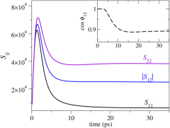
Fig. 4: Time dependence of the coefficients $\mathcal{S}_{ij}$. The inset shows the cosine of the phase angle $\phi_{12}$ as a function of time. Note that the $\mathcal{S}_{ij}$ tend to constant values in the limit $t\gg\tau_{c}=2.8$ ps as appropriate for CMB.

III.3 Analytics of noise-induced coherences and timescale for eigenstate formation

As shown in Figs. 2 and 3, the CBBR-induced coherent oscillations survive on a timescale much longer ($\sim$100 picoseconds) than the coherence time of CBBR at 2.7 K ($\hbar/kT=2.8$ ps). To explain this surprising longevity, we develop an analytical model for the time evolution of the coherences, based on Eq. (II). The model provides physical insight into the role of atomic energy levels, transition dipole moments, and the coherence time of the radiation, as they determine the coherent evolution of the Rydberg atom. In particular, the results show coherences that oscillate with the frequency determined by the energy level splitting, and coherence properties of the radiation that enter through the “phase shifts” and various prefactors that can be assumed to be constant in the long time limit ($t\gg\tau_{c}$).

We emphasize that the results obtained here apply to the temporal dynamics of any atomic and/or molecular system coupled to incoherent radiation that is described by an arbitrary stationary correlation function, including CBBR.

Introducing the complex coefficients

$$\mathcal{S}_{ij}(t)=\mathcal{K}_{0}^{(+)}(\omega_{i0},t)+\mathcal{K}_{0}^{(-)}(\omega_{j0},t)$$ (10)

and using the property $\mathcal{S}_{ij}^{*}=\mathcal{S}_{ji}$ which follows from the definition (4), we can rewrite the off-diagonal density matrix elements [ Eq. (II)] as

$$\rho_{ij}(t)=\frac{\langle\mu_{i0}\mu_{j0}^{*}\rangle_{p}}{\hbar^{2}}\frac{1}{\text{i}\omega_{ij}}[\mathcal{S}_{ij}^{*}-e^{-\text{i}\omega_{ij}t}\mathcal{S}_{ij}]$$ (11)

The coefficients $\mathcal{S}_{ij}$ are plotted in Fig. 4 as a function of time for a sample pair of eigenstates $|1\rangle=|66s\rangle$ and $|2\rangle=|67s\rangle$ populated by interaction with CMB starting from the $|65p\rangle$ initial Rydberg state (see Fig. 1). The states are separated by an energy gap of $\hbar\omega_{21}=0.86$ cm^-1 ($1/\omega_{21}=6.2$ ps). The correlation function $\mathcal{C}(\tau)$ of the blackbody radiation decays on the timescale $t_{c}\sim 3\tau_{c}\approx 10$ ps (see Appendix A). Accordingly, both the magnitudes and the phases of the coefficients $\mathcal{S}_{ij}=|\mathcal{S}_{ij}|e^{\text{i}\phi_{ij}}$ display time-dependent behavior during times $t<t_{c}$ (here $\sim$10-15 ps), after which ($t>t_{c}$) they can be well approximated by a constant (the constant $\mathcal{S}_{ij}$ approximation, see Fig. 4). Note that the diagonal matrix elements $\mathcal{S}_{ii}$ are real.

For the absolute value of the off-diagonal density matrix elements in Eq. (11), we find

$$|\rho_{ij}(t)|=\frac{|\langle\mu_{i0}\mu^{*}_{j0}\rangle_{p}|}{\hbar^{2}}\frac{|\mathcal{S}_{ij}|}{|\omega_{ij}|}2|\sin(\phi_{ij}-\omega_{ij}t/2)|$$ (12)

whereas the real and imaginary parts of the coherences are given by

$$\text{Re}\rho_{ij}(t) =-\frac{\langle\mu_{i0}\mu^{*}_{j0}\rangle_{p}}{\hbar^{2}}\frac{|\mathcal{S}_{ij}|}{\omega_{ij}}\left[\sin(\phi_{ij}-\omega_{ij}t)+\sin\phi_{ij}\right];$$

$$\text{Im}\rho_{ij}(t) =\frac{\langle\mu_{i0}\mu^{*}_{j0}\rangle_{p}}{\hbar^{2}}\frac{|\mathcal{S}_{ij}|}{\omega_{ij}}\left[\cos(\phi_{ij}-\omega_{ij}t)-\cos\phi_{ij}\right];$$ (13)

These expressions show that the absolute magnitude of the coherence oscillates with the frequency $\omega_{ij}/2$ determined by the energy splitting between the two eigenstates. The real and imaginary parts of the coherences oscillate at twice this frequency. A related result was obtained in Ref. Zaheen for the case of white noise. Equation (12) is, however, more general, as it applies to any kind of colored noise described by an arbitrary correlation function $C(\tau)$ (the only essential requirement being that the noise is stationary so that Eq. (II) applies). Each particular correlation function determines the dynamics through different $\mathcal{S}_{ij}$ coefficients in Eq. (11), which contains the characteristics of the radiation.

Equations (III.3) provide convenient analytic expressions for noise-induced coherences in the limit $t\gg\tau_{c}$, and are straightforward to parametrize via the coefficients $\mathcal{S}_{ij}$. We note that these expressions could significantly reduce computational challenges in, e.g., calculating the density matrix dynamics of molecular systems. Figure 5(a) shows the real part of the coherence $\rho_{12}(t)$ calculated using Eq. (III.3) parametrized by the constant, asymptotic values for $|\mathcal{S}_{12}|$ and $\phi_{12}$ from Fig. 4. The analytic result is in excellent agreement with the exact calculation, thereby validating the constant $\mathcal{S}_{ij}$ approximation. The disagreement at short times is expected, since the $\mathcal{S}_{ij}$ vary strongly in this region, and hence cannot be approximated by constants. In particular, Eqs. (III.3) parametrized by the asymptotic values of $\mathcal{S}_{ij}$ disagrees with the correct zero-time result $\rho_{ij}(0)=0$. This drawback can be remedied, if desired, by using a different parametrization such that $\mathcal{S}_{ij}(t)\to 0$ as $t\to 0$.

A useful measure of the relative importance of coherences and populations is the ratio Zaheen

$$\mathcal{C}_{ij}(t)=\frac{|\rho_{ij}(t)|}{\rho_{ii}(t)+\rho_{jj}(t)}$$ (14)

A small value of $\mathcal{C}_{ij}$ indicates that the magnitude of the coherence $\rho_{ij}$ is small compared to that of the populations, which is characteristic of a nearly pure statistical mixture. Hence, the timescale for the decay of $\mathcal{C}$ can be used to quantify the evolution from a purely coherent state at $t=0$ to a statistical mixture of stationary eigenstates.

To obtain an analytic expression for the $\mathcal{C}$-ratio, we use an approximate result for state populations obtained from Eq. (II) by omitting the $\mathcal{K}_{1}^{(\pm)}$ terms, which are negligible compared to the other two terms in the limit $t\gg\tau_{c}$ TBP . Combining the resulting expression with Eq. (12), we find

$$\mathcal{C}_{ij}(t)=\frac{1}{|\omega_{ij}|t}\frac{|\langle\mu_{i0}\mu_{j0}\rangle_{p}|}{\langle|\mu_{i0}|^{2}\rangle_{p}\mathcal{S}_{ii}+\langle|\mu_{j0}|^{2}\rangle_{p}\mathcal{S}_{jj}}|\mathcal{S}_{ij}|\\ \times 2|\sin(\phi_{ij}-\omega_{ij}t/2)|$$ (15)

Figure 5(b) plots the time variation of the $\mathcal{C}$-ratio for the Rydberg states $|1\rangle$ and $|2\rangle$ defined above. It is seen to decay in time as $1/(|\omega_{ij}|t)$ and oscillates with the frequency $\omega_{ij}/2$, due to the oscillating behavior of the absolute magnitude of the coherence (12). This shows that the coherences between the Rydberg levels, evident in Figs. 2 and 3, survive for long times because of the small energy splittings between the levels populated by one-photon absorption and stimulated emission of CBBR. Longevity of coherences in association with small energy level splittings has been noted before, albeit in different contexts and with different functional dependences on the splittingsElran1 ; Elran2 ; Pachonjpcl Indeed, in this case, the dependence on $\omega_{ij}t$ is reminiscent of the energy-time uncertainty principle, as the system strives, in time, to perceive individual energy levels.

IV Summary and future prospects

In summary, the long-lived temporal coherence, and associated decoherence, in Rydberg atoms induced by the sudden turn-on of CBBR at 2.7 K has been examined. The physical mechanism behind the coherences and their slow decay is the long coherence time of CBBR and the small energy level splittings of the Rydberg levels excited by the CMB. The large transition dipole moments of the Rydberg atoms make these coherences manifest in various physical observables. Directly measuring CMB coherence properties via fluorescence detection would require 90 dB amplification of the incident CMB signal, beyond current practice of 67 dB. At present, achieving such a high gain experimentally over a broad frequency interval (10-20 GHz) is a formidable challenge. However, recent developments in amplification technology allow for higher gains over much wider frequency intervals than possible with HEMT amplifiers NatPhys , and these may resolve experimental challenges associated with carrying out the proposed experiment.

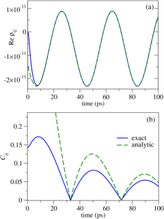
Fig. 5: (a) The real part of the coherence between levels $|1\rangle=|66s\rangle$ and $|2\rangle=|67s\rangle$ as a function of time. Full line – exact result (Eq. (5), Fig. 2), dashed line – constant $\mathcal{S}_{ij}$ approximation (Eq. III.3). (b) The ratio $\mathcal{C}_{12}=|\rho_{12}(t)|/(\rho_{11}(t)+\rho_{22}(t))$ as a function of time. Full line – exact result, dashed line – constant $\mathcal{S}_{12}$ approximation, Eq. (15).

Finally, we note that the long-lived coherences shown in Fig. 2 can also be observed with any experimental technique that is sensitive to coherent superpositions of the atom’s excited states. Examples include selective field ionization RA , photoionization RA , and half-cycle pulse ionization Jones . The former technique also provides a direct route to measuring non-Markovian deviations from the linear behavior of state populations at short times (Fig. 2a), which also relates to the coherence properties of CBBR TBP .

One extension of this work is readily motivated. The study in this paper has examined the sudden turn-on associated with a single state prepared in an excited Rydberg state. However, slower preparation of Rydberg states, e.g., using a 15 ps laser pulse is expected to produce RydbergWP additional interesting results. That is, such a pulse prepares a coherent superposition of five eigenstates centered around $n=65$, rather than a single state, as assumed above. This superposition will then couple, via the CMB, to adjacent $s$ and $p$ Rydberg states. Fluorescence from this collection of levels is then expected to display a more complicated pattern of quantum beats than described above, which then decoheres in time. In addition, since the initial state is then a prepared superposition of energy eigenstates, decay of decoherence on assorted time scales is also anticipated Elran1 ; Elran2 . Further, one can consider modifying the laser pulse shape in order to enhance the quantum beat signal. Such studies are underway.

V Acknowledgements

We thank Dr. Marian Pospieszalski, Dr. Hossein Sadeghpour, Prof. John Polanyi, Dr. Colin Connoly and Dr. Leonardo Pachón for discussions. This work was supported by the Natural Sciences and Engineering Research Council of Canada and the U.S. Air Force Office of Scientific Research under contract number FA9550-13-1-0005.

VI Appendix

This Appendix outlines the derivation of the equations of motion for the density matrix [Eqs. (3) and (5)] that describe the interaction of a Rydberg atom with blackbody radiation.

The time evolution of the density matrix for a Rydberg atom interacting with CBBR is given by Eq. (1). For a stationary CBBR source, the correlation function $\mathcal{C}(\tau^{\prime},\tau^{\prime\prime})$ is a function of $\tau=\tau^{\prime}-\tau^{\prime\prime}$ only. The absolute value and the phase of the CBBR correlation function given by Eq. (2) are plotted in Fig. 6 as a function of $\tau$ for $T_{\text{CMB}}=2.718$ K KanoWolf .

By changing the integration variables $\tau_{\pm}=\tau^{\prime}\pm\tau^{\prime\prime}$, Eq. (1) can be recast in the form

$$\rho_{ij}(t)=\frac{\langle\mu_{i0}\mu_{j0}^{*}\rangle_{p}}{\hbar^{2}}e^{-\text{i}\omega_{ij}t}\frac{1}{2}\biggl{[}\int_{-t}^{0}d\tau_{-}\int_{-\tau_{-}}^{\tau_{-}+2t}d\tau_{+}f(\tau_{+},\tau_{-})\\ +\int_{0}^{t}d\tau_{-}\int_{\tau_{-}}^{2t-\tau_{-}}d\tau_{+}f(\tau_{+},\tau_{-})\biggr{]},$$ (16)

where $f(\tau_{+},\tau_{-})=\mathcal{C}(\tau_{-})e^{\text{i}\omega_{i0}(\tau_{+}+\tau_{-})/2}e^{-\text{i}\omega_{j0}(\tau_{+}-\tau_{-})/2}$. For $i=j$, the integrand simplifies to

$$f(\tau_{-})=\mathcal{C}(\tau_{-})e^{\text{i}\omega_{i0}\tau_{-}}$$ (17)

allowing the integration over $\tau_{+}$ in Eq. (16) to be performed analytically to yield the population dynamics

$$\rho_{ii}(t)=\frac{\langle|\mu_{i0}|^{2}\rangle_{p}}{\hbar^{2}}\left[t\mathcal{I}_{0}(t)+\mathcal{I}_{1}(t)\right]$$ (18)

with

$$\mathcal{I}_{0}(t) =\int_{-t}^{t}f(\tau_{-})d\tau_{-};$$ (19)

$$\mathcal{I}_{1}(t) =\int_{-t}^{0}\tau_{-}[f(\tau_{-})+f(-\tau_{-})]d\tau_{-}$$ (20)

Splitting the range of integration in the first term on the right-hand side into positive and negative $\tau_{-}$ regions, relabeling the integration variable $\tau_{-}\to\tau$, and using Eq. (17) we find

$$\mathcal{I}_{0}(t)=\int_{0}^{t}[\mathcal{C}(\tau)e^{\text{i}\omega_{i0}\tau}+\mathcal{C}(-\tau)e^{-\text{i}\omega_{i0}\tau}]d\tau$$ (21)

and

$$\mathcal{I}_{1}(t)=-\int_{0}^{t}\tau[\mathcal{C}(\tau)e^{\text{i}\omega_{i0}\tau}+\mathcal{C}(-\tau)e^{-\text{i}\omega_{i0}\tau}]d\tau.$$ (22)

Introducing the half-Fourier transforms

$$\mathcal{K}^{(\pm)}_{0}(\omega,t) =\int_{0}^{t}\mathcal{C(\pm\tau)}e^{\pm\text{i}\omega\tau}d\tau$$ (23)

$$\mathcal{K}^{(\pm)}_{1}(\omega,t) =\int_{0}^{t}\tau\mathcal{C(\pm\tau)}e^{\pm\text{i}\omega\tau}d\tau,$$ (24)

we obtain Eq. (3) in the text.

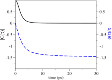
Fig. 6: Time dependence of CBBR correlation function $\mathcal{C}(\tau)=|\mathcal{C}(\tau)|e^{\text{i}\phi(\tau)}$ for $T=2.718$ K (in units of $\mathcal{E}_{0}^{2}$, see Eq.  (2) of the main text). Full line – absolute magnitude ($|\mathcal{C}(\tau)|$), dashed line – phase ($\phi(\tau)/\pi$) KanoWolf .

In the case of $i\neq j$ (off-diagonal elements of the density matrix), the integrand depends on both $\tau_{+}$ and $\tau_{-}$ via

$$f(\tau_{+},\tau_{-})=\mathcal{C}(\tau_{-})e^{\text{i}\tau_{+}(\omega_{i0}-\omega_{j0})/2}e^{\text{i}\tau_{-}(\omega_{i0}+\omega_{j0})/2}$$ (25)

Substituting Eq. (25) in Eq. (16) and evaluating the integral over $\tau_{+}$ analytically (which is straightforward since $\mathcal{C}(\tau_{-})$ is a function of $\tau_{-}$ only), we arrive at the result

$$\rho_{ij}(t)=\frac{\langle\mu_{i0}\mu_{j0}^{*}\rangle_{p}}{\hbar^{2}(\text{i}\omega_{ij})}\biggl{\{}\int_{0}^{t}\left[\mathcal{C}(\tau)e^{\text{i}\omega_{j0}\tau}+\mathcal{C}(-\tau)e^{-\text{i}\omega_{i0}\tau}\right]d\tau\\ -e^{-\text{i}\omega_{ij}t}\int_{0}^{t}\left[\mathcal{C}(\tau)e^{\text{i}\omega_{i0}\tau}+\mathcal{C}(-\tau)e^{-\text{i}\omega_{j0}\tau}\right]d\tau\biggr{\}}$$ (26)

With the help of the definition (23), we obtain Eq. (5) in the above text.

$$\zeta(4,a)=\frac{1}{\Gamma(4)}\int_{0}^{\infty}\frac{x^{3}e^{-ax}}{1-e^{-x}}dx,$$ (27)

where $\Gamma(x)$ is a Gamma function, we get

$$\rho_{ii}(t\to\infty)=\frac{\langle|\mu_{i0}|^{2}\rangle_{p}}{\hbar^{2}}\int_{-\infty}^{\infty}\mathcal{C}(\tau)e^{\text{i}\omega_{i0}\tau}d\tau\\ =\mathcal{E}_{0}^{2}\frac{90}{\pi^{4}\Gamma(4)}\int_{0}^{\infty}d\omega\frac{\omega^{3}e^{-(1+\text{i}\lambda\tau)\omega}}{1-e^{-\omega}}\int_{-\infty}^{\infty}d\tau e^{-\text{i}\lambda\tau\omega}e^{\text{i}\omega_{i0}\tau}$$ (28)

The integral over $\tau$ is readily evaluated in terms of the Dirac $\delta$-function ($\int_{-\infty}^{\infty}e^{-\text{i}(\lambda\omega-\omega_{i0})\tau}d\tau=2\pi\delta(\lambda\omega-\omega_{i0}).$) and Eq. (28) reduces to the Fermi Golden Rule result given by Eq. (4) in the text ($\lambda=kT/\hbar$)

$$\rho_{ii}(t\to\infty) =\mathcal{E}_{0}^{2}\langle|\mu_{i0}|^{2}\rangle_{p}\frac{90}{\pi^{4}}\frac{2\pi}{\Gamma(4)}\frac{1}{\lambda^{4}}\frac{\omega_{i0}^{3}}{e^{\omega_{i0}/\lambda}-1}t$$

$$=\frac{4\langle|\mu_{i0}|^{2}\rangle_{p}}{3\hbar c^{3}}\frac{\omega_{i0}^{3}}{e^{\hbar\omega_{i0}/kT}-1}t$$ (29)

Note that the proportionality coefficient in the second line of Eq. (VI) is the BBR-induced transition rate $W_{0\to i}$.

References

- (1) G. S. Engel, T. R. Calhoun, E. L. Read, T.-K. Ahn, T. Mancal, Y.-C. Cheng, R. E. Blankenship, and G. R. Fleming, Nature (London) 446, 782 (2007).
- (2) E. Collini, C. Y. Wong, K. E. Wilk, P. M. G. Curmi, P. Brumer, and G. D. Scholes, Nature (London) 463, 644 (2010).
- (3) G. D. Scholes, J. Phys. Chem. Lett. 1, 2 (2010).
- (4) P. Brumer and M. Shapiro, Proc. Natl. Acad. Sci. USA 109, 19575 (2012).
- (5) M. O. Scully, K. R. Chapin, K.E. Dorfman, M. B. Kim, and A. Svidzinsky, Proc. Natl. Acad. Sci. USA 108, 15097 (2011).
- (6) T. Middelmann, S. Falke, C. Lisdat, and U. Sterr, Phys. Rev. Lett. 109, 263004 (2012); M. S. Safronova, S. G. Porsev, U. I. Safronova, M. G. Kozlov, and C. W. Clark, Phys. Rev. A 87, 012509 (2013).
- (7) V.D. Ovsiannikov, A. Derevianko and K. Gibble, Phys. Rev. Lett. 107, 093003 (2011).
- (8) T. F. Gallagher, Rydberg Atoms (Cambridge University Press, Cambridge, 1994).
- (9) S. Hoekstra, J. J. Gilijamse, B. Sartakov, N. Vanhaecke, L. Scharfenberg, S. Y. T. van de Meerakker, and G. Meijer, Phys. Rev. Lett. 98, 133001 (2007).
- (10) J.W. Farley and W. H. Wing, Phys. Rev. A 23, 2397 (1981); L. Hollberg and J. L. Hall, Phys. Rev. Lett. 53, 230 (1984); T. Nakajima, P. Lambropoulos, and H. Walther, Phys. Rev. A 56, 5100 (1997).
- (11) W. P. Spencer, A. G. Vaidyanathan, D. Kleppner, and T. W. Ducas, Phys. Rev. A 25, 380 (1982); J. M. Raimond, P. Goy, M. Gross, C. Fabre, and S. Haroche, Phys. Rev. Lett. 49, 117 (1982).
- (12) M. Tada, Y. Kishimoto, K. Kominato, M. Shibata et al., Phys. Lett. A 349, 488 (2006).
- (13) R. G. Hulet, E. S. Hilfer, and D. Kleppner, Phys. Rev. Lett. 55, 2137 (1985).
- (14) A. Mari and J. Eisert, Phys. Rev. Lett. 108, 120602 (2012); B. Cleuren, B. Rutten, and C. Van den Broeck, Phys. Rev. Lett. 108, 120603 (2012).
- (15) L. Mandel and E. Wolf, Optical Coherence and Quantum Optics (Cambridge University Press, Cambridge, 1995), Chap. 13.
- (16) C. L. Mehta and E. Wolf, Phys. Rev. 134, A1143 (1964); Phys. Rev. 134, A1149.
- (17) Y. Kano and E. Wolf, Proc. Phys. Soc. 80, 1273 (1962).
- (18) L. A. Pachón and P. Brumer, Phys. Rev. A 87, 022106 (2013).
- (19) K. Hoki and P. Brumer, Procedia Chem. 3, 122 (2011).
- (20) Z. Sadeq, M.Sc. thesis, University of Toronto, 2012; Z. Sadeq and P. Brumer, to be submitted (2013).
- (21) X.-P. Jiang and P. Brumer, J. Chem. Phys. 94, 5833 (1991); Chem. Phys. Lett. 180, 222 (1991).
- (22) P. D. Naselsky, D. I. Novikov, and I. D. Novikov, The Physics of the Cosmic Microwave Background (Cambridge University Press, Cambridge, 2006).
- (23) Coherent HEMT amplifiers are capable of large gains in the 20 GHz region of interest. See, e.g., Table 3 of N. Jarosik et al., Astrophys. J. Suppl. Series 145, 413 (2003), which describes the WMAP CMB amplification system consisting of two amplifiers, one radiatively cooled and the other at room temperature. As clarified by M. Pospieszalski in a private communication, the total gain of the two-amplifier chain is 67 dB).
- (24) S. Weinberg, Cosmology, (Oxford University Press, Oxford, 2008).
- (25) G. Hinshaw et al., Astrophys. J. Suppl. Ser. 180, 225 (2009); E. Komatsu et al., Astrophys. J. Suppl. Ser. 180, 330 (2009).
- (26) R. Amanullah et al., Astrophys. J. 716, 712 (2010).
- (27) R. Hakim, Ann. Phys. (Paris) 4, 217 (1979).
- (28) T. V. Tscherbul, L.A. Pachón and P. Brumer (manuscript in preparation).
- (29) H.-P. Breuer and F. Petruccione, The Theory of Open Quantum Systems (Clarendon Press, Oxford, 2006), Chap. 3.4.
- (30) D. J. Griffiths, Introduction to Quantum Mechanics (Prentice Hall, NJ, 1995), Chap. 9.2.
- (31) W. M. Itano, L. L. Lewis, and D. J. Wineland, Phys. Rev. A 25, 1233 (1982).
- (32) I. I. Beterov, I. I. Ryabtsev, D. B. Tretyakov, and V. M. Entin, Phys. Rev. A 79, 052504 (2009); Phys. Rev. A 80, 059902(E) (2009).
- (33) M. L. Zimmerman, M. G. Littman, M. M. Kash, and D. Kleppner, Phys. Rev. A 20, 2251 (1979).
- (34) B. H. Eom, P. K. Day, H. G. LeDuc, and J. Zmuidzinas, Nature Phys. 8, 623 (2012).
- (35) J. A. Yeazell, M. Mallalieu, and C. R. Stroud, Jr. Phys. Rev. Lett. 64, 2007 (1990); T. F. Gallagher, Phys. Scr. 76, C145 (2007).
- (36) Y. Elran and P. Brumer, J. Chem. Phys. 121, 2673 (2004).
- (37) Y. Elran and P. Brumer, J. Chem. Phys. 138, 234308 (2013).
- (38) M. Schlosshauer, Decoherence and the Quantum-to-Classical Transition (Springer-Verlag, Berlin, 2008), Chap. 2.4.
- (39) T. A. Grinev and P. Brumer, to be published.
- (40) W. Demtröder, Atoms, Molecules and Photons, 2nd ed. (Springer-Verlag Berlin Heidelberg, 2010), Chap. 7.
- (41) L.A. Pachón and P. Brumer, J. Phys. Chem. Lett. 2, 2728 (2011).
- (42) R. R. Jones, Phys. Rev. Lett. 76, 3927 (1996).