Searches for Large-Scale Anisotropies of Cosmic Rays :
Harmonic Analysis and Shuffling Technique

Abstract

The measurement of large scale anisotropies in cosmic ray arrival directions is generally performed through harmonic analyses of the right ascension distribution as a function of energy. These measurements are challenging due to the small expected anisotropies and meanwhile the relatively large modulations of observed counting rates due to experimental effects. In this paper, we present a procedure based on the shuffling technique to carry out these measurements, applicable to any cosmic ray detector without any additional corrections for the observed counting rates.

1 Introduction

In investigating the origin of cosmic rays, the measurement of anisotropy in the arrival directions is an important tool, complementary to the energy spectrum and mass composition. From the observational point of view indeed, the study of the cosmic ray anisotropy with energy is closely connected to the problem of cosmic ray propagation and sources. Due to the scattering of cosmic rays in the Galactic magnetic field, the anisotropy imprinted in arrival directions is mainly expected at large scales up to the highest energies. The experimental study of large scale anisotropies is thus fundamental for cosmic ray physics, though it is challenging.

At energies greater than $10^{13}$ eV, cosmic ray measurements are indirect due to the low primary intensity, and are usually performed through extensive air showers with surface array detectors, Cherenkov telescopes, or fluorescence telescopes. Surface array detectors with high duty cycle operate almost uniformly with respect to sidereal time thanks to the rotation of the Earth. In contrast, the low duty cycle of Cherenkov and fluorescence telescopes, operating only on dark nights, propagates into large variations of exposure with sidereal time. These variations, almost always larger than the expected anisotropies, induce artificial modulations of the cosmic ray intensity in local sidereal time, and thus make delicate the measurements of harmonics in the right ascension distribution - in particular for the first harmonic.

The most commonly used technique to search for large scale anisotropies is the analysis in right ascension only, through harmonic analysis (referred to as Rayleigh formalism) of the event counting rate [1]. The technique itself is rather simple, but the greatest difficulties are in the estimation of the directional exposure of the experiment. For any energy range, the directional exposure $\tilde{\omega}(\delta,\alpha)$ provides the effective time-integrated collecting area for a flux from each declination $\delta$ and right ascension $\alpha$ :

$$\tilde{\omega}(\delta,\alpha)=A~{}\int\mathrm{d}T~{}F(\theta(T-\alpha,\delta),\varphi(T-\alpha,\delta),T).$$ (1)

Here, $T$ stands for the local sidereal time, and $A$ stands for the total collecting area of the experiment. The function $F(\theta,\varphi,T)$ encompasses geometrical aperture and detection efficiency effects under incidence zenith angle $\theta$ and azimuth angle $\varphi$. The explicit dependence of $F$ on local sidereal time $T$ is due to the unavoidable variations of the on-time of the detectors. In addition, extensive air showers properties are affected by meteorological modulations of the air density (through variations of the Molière radius) and of the pressure (due to the absorption of the electromagnetic component) [2, 3]. This can produce a seasonal variation of the diurnal counting rate, which then results in an artificial modulation of the intensity in local sidereal time [4]. The accurate control of all these effects is challenging in the case of surface array detectors, and generally out of reach in cases of Cherenkov and fluorescence telescopes. Note that, when searching for large-scale anisotropies in right ascension only, the directional exposure $\omega(\alpha)$ integrated in declination is in fact the quantity of interest :

$$\omega(\alpha)=\int\mathrm{d}\delta\cos{\delta}~{}\tilde{\omega}(\delta,\alpha).$$ (2)

Throughout the paper, the use of ’directional exposure’ will mainly refer to as $\omega(\alpha)$ - except in sections 2.4 and 2.5 where explicit references to $\tilde{\omega}(\delta,\alpha)$ will be needed. In addition, the relative directional exposure $\omega_{r}(\alpha)$ will be also useful, defined as $\omega_{r}(\alpha)=\omega(\alpha)/\epsilon$, with $\epsilon$ the total exposure divided by $2\pi$.

In contrast to large scale anisotropy searches, point-like source searches can be carried out by overcoming the explicit estimation of the $F$ function through the use of the shuffling method [5]. This method only makes use of the observed data set for determining the number of background events in any direction of the sky, through the generation of simulation data sets in which the actual event times are randomly associated with the actual local angles. In this way, the counting rate variations are naturally accounted for in each simulation data set, because all background events have the same time distribution as real events. In addition, preserving the local angle distribution as observed in the actual data set guarantees a proper modelling of the detection efficiency in a total empirical manner. However, since events from eventual excesses are used to estimate the background level, the background estimate is necessarily overestimated compared to the true background [5, 6]. While this effect is negligible when searching for point sources, it is expected to be important when searching for diffuse excesses and in particular for large scale patterns [7, 8].

This paper is dedicated to explore in a comprehensive way the performances of the shuffling method when searching for large scale anisotropies in right ascension. Compared to previous studies, a new interpretation of the directional exposure function as estimated when applying the shuffling method is given, together with a complete procedure for interpreting the derived anisotropy amplitudes and for converting them into the corresponding anisotropy components in the equatorial plane. To this aim, the general formalism of harmonic analysis is first presented in section 2, with a special attention given to the recovering of the harmonic coefficients in the case of large variations of the directional exposure of the experiment in right ascension. The principle of the shuffling technique and its application to large scale anisotropy searches are then presented in section 3. It is shown that some anisotropy can be recovered while properly accounting for any spurious effect of experimental origin. The performances of this technique are given in section 4 before to conclude in section 5.

2 Harmonic analysis in right ascension

Harmonic analysis of the right ascension distribution of cosmic rays in different energy ranges is a powerful tool for picking up and for characterising any modulation in this coordinate. Any angular distribution, $\Phi(\alpha)$, can be decomposed in terms of a harmonic expansion :

$$\Phi(\alpha)=a_{0}+\sum_{n>0}~{}a_{n}^{c}~{}\cos{n\alpha}+\sum_{n>0}~{}a_{n}^{s}~{}\sin{n\alpha}.$$ (3)

The customary recipe to extract each harmonic coefficient makes use of the orthogona- lity of the trigonometric functions :

$$a_{0} = \frac{1}{2\pi}\int_{0}^{2\pi}\mathrm{d}\alpha~{}\Phi(\alpha),$$

$$a_{n}^{c} = \frac{1}{\pi}\int_{0}^{2\pi}\mathrm{d}\alpha~{}\Phi(\alpha)~{}\cos{n\alpha},$$

$$a_{n}^{s} = \frac{1}{\pi}\int_{0}^{2\pi}\mathrm{d}\alpha~{}\Phi(\alpha)~{}\sin{n\alpha}.$$ (4)

In this section, we remind how this standard formalism can be applied to any set of arrival directions $\{\alpha_{1},...,\alpha_{N}\}_{1\leq i\leq N}$ in the case of a purely uniform or a slightly non-uniform directional exposure, and present how to proceed in the case of a highly non-uniform directional exposure. Hereafter, we use an over-line to indicate the estimator of any quantity.

2.1 Uniform directional exposure

In the case of a purely uniform directional exposure, the Rayleigh formalism [1] directly provides the amplitude of the different harmonics, the corresponding phase (i.e. right ascension of the maximum of intensity), and the probability of detecting a signal due to fluctuations of an isotropic distribution with an amplitude equal or larger than the observed one. The observed arrival direction distribution, $\overline{\Phi}(\alpha)$, is here modelled as a sum of Dirac functions over the circle, $\overline{\Phi}(\alpha)=\sum_{i}\delta(\alpha,\alpha_{i})$, so that integrations in equation 2 reduce to discrete sums :

$$\overline{a}_{n}^{c} = \frac{2}{N}\sum_{1\leq i\leq N}\cos{n\alpha_{i}},$$

$$\overline{a}_{n}^{s} = \frac{2}{N}\sum_{1\leq i\leq N}\sin{n\alpha_{i}}.$$ (5)

Here, the re-calibrated harmonic coefficients $a_{n}^{c}\equiv a_{n}^{c}/a_{0}$ and $a_{n}^{s}\equiv a_{n}^{s}/a_{0}$ are directly considered, as it is traditionally the case in measuring relative anisotropies.

The statistical properties of the estimators $\{\overline{a}_{n}^{c},\overline{a}_{n}^{s}\}$ can be derived from the Poissonian nature of the sampling of $N$ points over the circle distributed according to the underlying angular distribution $\Phi(\alpha)$. From Poisson statistics indeed, the first and second moments of $\overline{\Phi}(\alpha)$ averaged over a large number of realisations of $N$ events read :

$$\left\langle\overline{\Phi}(\alpha)\right\rangle = \epsilon\Phi(\alpha),$$

$$\left\langle\overline{\Phi}(\alpha)\overline{\Phi}(\alpha^{\prime})\right\rangle = \epsilon^{2}\Phi(\alpha)\Phi(\alpha^{\prime})+\epsilon\Phi(\alpha)\delta(\alpha,\alpha^{\prime}).$$ (6)

Propagating these properties into the first and second moments of the estimators $\{\overline{a}_{n}^{c},\overline{a}_{n}^{s}\}$ leads, on the one hand, to unbiased estimators :

$$\left\langle\overline{a}_{n}^{c}\right\rangle = a_{n}^{c},$$

$$\left\langle\overline{a}_{n}^{s}\right\rangle = a_{n}^{s},$$ (7)

and, on the other hand, to the following covariance matrix :

$$\mathrm{cov}(\overline{a}_{m}^{c},\overline{a}_{n}^{c}) = \frac{1}{\epsilon\pi^{2}a_{0}^{2}}\int\mathrm{d}\alpha~{}\Phi(\alpha)~{}\cos{m\alpha}~{}\cos{n\alpha},$$

$$\mathrm{cov}(\overline{a}_{m}^{s},\overline{a}_{n}^{s}) = \frac{1}{\epsilon\pi^{2}a_{0}^{2}}\int\mathrm{d}\alpha~{}\Phi(\alpha)~{}\sin{m\alpha}~{}\sin{n\alpha},$$

$$\mathrm{cov}(\overline{a}_{m}^{c},\overline{a}_{n}^{s}) = \frac{1}{\epsilon\pi^{2}a_{0}^{2}}\int\mathrm{d}\alpha~{}\Phi(\alpha)~{}\cos{m\alpha}~{}\sin{n\alpha}.$$ (8)

In case of small anisotropies (i.e. $|a_{n}^{c}/a_{0}|\ll 1$ and $|a_{n}^{s}/a_{0}|\ll 1$), and with $N$ a good estimator of $\epsilon a_{0}$, the previous expressions allow the derivation of the RMS of the estimators as :

$$\sigma_{n}^{c}(\overline{a}_{n}^{c})=\sigma_{n}^{s}(\overline{a}_{n}^{s})=\bigg{(}\frac{2}{N}\bigg{)}^{0.5}.$$ (9)

For an isotropic realisation, $\overline{a}_{n}^{c}$ and $\overline{a}_{n}^{s}$ are random variables whose joint p.d.f., $p_{A_{n}^{c},A_{n}^{s}}$, can be factorised in the limit of large number of events in terms of two Gaussian distributions whose variances are thus $\sigma^{2}=2/N$. For any $n$, the joint p.d.f. of the estimated amplitude, $\overline{r}_{n}=(\overline{a}_{n}^{c2}+\overline{a}_{n}^{s2})^{1/2}$, and phase, $\overline{\phi}_{n}=\arctan{(\overline{a}_{n}^{s}/\overline{a}_{n}^{c})}$, is then obtained through the Jacobian transformation :

$$p_{R_{n},\Phi_{n}}(\overline{r}_{n},\overline{\phi}_{n}) = \left|\frac{\partial(\overline{a}_{n}^{c},\overline{a}_{n}^{s})}{\partial(\overline{r}_{n},\overline{\phi}_{n})}\right|~{}p_{A_{n}^{c},A_{n}^{s}}(\overline{a}_{n}^{c}(\overline{r}_{n},\overline{\phi}_{n}),\overline{a}_{n}^{s}(\overline{r}_{n}),\overline{\phi}_{n})$$ (10)

$$= \frac{\overline{r}_{n}}{2\pi\sigma^{2}}~{}\exp{(-\overline{r}_{n}^{2}/2\sigma^{2})}.$$

From this expression, it is straightforward to recover the Rayleigh distribution for the p.d.f. of the amplitude, $p_{R_{n}}$, and the uniform distribution between 0 and $2\pi$ for the p.d.f. of the phase, $p_{\Phi_{n}}$.

2.2 Non-uniform directional exposure

The Rayleigh formalism aforementioned can be applied off the shelf only in the case of a purely uniform directional exposure. This ideal condition is generally not fulfilled, so that formally, the integrations performed in equation 2 do not allow any longer a direct extraction of the harmonic coefficients of $\Phi(\alpha)$. We assume they allow the extraction of the product $\omega(\alpha)\Phi(\alpha)$, and will come back on the conditions of validity of this assumption in sub-section 2.4.

At the sidereal time scale, the directional exposure of most observatories operating with high duty cycle (e.g. surface detector arrays) is however only moderately (or even slightly) non-uniform. A simple recipe to account for the variations of $\omega(\alpha)$ is then to transform the observed angular distribution $\overline{\Phi}(\alpha)$ into the one that would have been observed with an uniform directional exposure : $\overline{\Phi}(\alpha)/\omega(\alpha)$ [9]. In that way, discrete summations in equation 2.1 are changed into :

$$\overline{a}_{n}^{c} = \frac{2}{\tilde{N}}\sum_{1\leq i\leq N}\frac{\cos{n\alpha_{i}}}{\omega(\alpha_{i})},$$

$$\overline{a}_{n}^{s} = \frac{2}{\tilde{N}}\sum_{1\leq i\leq N}\frac{\sin{n\alpha_{i}}}{\omega(\alpha_{i})},$$ (11)

with $\tilde{N}=\sum_{i}~{}1/\omega(\alpha_{i})$.

The statistical properties of these estimators can be estimated in the same way as in the previous sub-section. The starting point is to consider the first and second moments of $\overline{\Phi}(\alpha)/\omega(\alpha)$ :

$$\left\langle\frac{\overline{\Phi}(\alpha)}{\omega(\alpha)}\right\rangle = \Phi(\alpha),$$

$$\left\langle\frac{\overline{\Phi}(\alpha)}{\omega(\alpha)}\frac{\overline{\Phi}(\alpha^{\prime})}{\omega(\alpha^{\prime})}\right\rangle = \Phi(\alpha)\Phi(\alpha^{\prime})+\frac{\Phi(\alpha)}{\omega(\alpha)}\delta(\alpha,\alpha^{\prime}).$$ (12)

In case of small anisotropies, this leads to the following expressions for the RMS of the estimators :

$$\sigma_{n}^{c} = \bigg{(}\frac{2}{N}\frac{1}{\pi}\int_{0}^{2\pi}\frac{\mathrm{d}\alpha}{\omega_{r}(\alpha)}\cos^{2}{n\alpha}\bigg{)}^{0.5},$$

$$\sigma_{n}^{s} = \bigg{(}\frac{2}{N}\frac{1}{\pi}\int_{0}^{2\pi}\frac{\mathrm{d}\alpha}{\omega_{r}(\alpha)}\sin^{2}{n\alpha}\bigg{)}^{0.5}.$$ (13)

The joint p.d.f. $p_{A_{n}^{c},A_{n}^{s}}$ under isotropy is now the product of two Gaussian with two distinct parameters $\sigma_{n}^{c}$ and $\sigma_{n}^{s}$. After the Jacobian transformation to get at the joint p.d.f. $p_{R_{n},\Phi_{n}}$, the integration over $\overline{\phi}_{n}$ yields the $p_{R_{n}}$ p.d.f. :

$$p_{R_{n}}(\overline{r}_{n})=\frac{\overline{r}_{n}}{\sigma_{n}^{c}\sigma_{n}^{s}}~{}\exp{\bigg{(}-\frac{{\sigma_{n}^{c}}^{2}+{\sigma_{n}^{s}}^{2}}{4{\sigma_{n}^{c}}^{2}{\sigma_{n}^{s}}^{2}}\overline{r}_{n}^{2}\bigg{)}}~{}I_{0}\bigg{(}\frac{{\sigma_{n}^{c}}^{2}-{\sigma_{n}^{s}}^{2}}{4{\sigma_{n}^{c}}^{2}{\sigma_{n}^{s}}^{2}}\overline{r}_{n}^{2}\bigg{)},$$ (14)

where $I_{0}(\cdot)$ is the modified Bessel function of first kind with order 0. This p.d.f. can be viewed as a generalisation of the Rayleigh distribution in the case of non-equal resolutions for the underlying Gaussian variables $\overline{a}_{n}^{c}$ and $\overline{a}_{n}^{s}$. The probability of detecting a signal due to fluctuations of an isotropic distribution with an amplitude equal or larger than the observed one can be obtained by integrating numerically $p_{R_{n}}$ above the observed value $\overline{r}_{n}$. On the other hand, the integration over $\overline{r}_{n}$ yields the $p_{\Phi_{n}}$ p.d.f. :

$$p_{\Phi_{n}}(\overline{\phi}_{n})=\frac{\sigma_{n}^{c}\sigma_{n}^{s}}{2\pi}\frac{1}{{\sigma_{n}^{c}}^{2}\sin^{2}{\overline{\phi}_{n}}+{\sigma_{n}^{s}}^{2}\cos^{2}{\overline{\phi}_{n}}}.$$ (15)

There are thus preferential directions for the reconstructed phases, fixed by the ratio between ${\sigma_{n}^{c}}^{2}$ and ${\sigma_{n}^{s}}^{2}$ - independently of the number of events.

This formalism is the relevant one in most of practical cases. It is to be noted, however, that variations of few percents in the directional exposure $\omega$ have no real numerical impact in equations 2.2 (and so in equations 14 and 15), so that in such cases, the p.d.f. of the amplitude can be approximated to a high level by the Rayleigh distribution, while the one of the phase by a uniform distribution.

2.3 Highly non-uniform directional exposure

Though the directional exposure of most observatories is generally only moderately non-uniform at the sidereal time scale, it is often useful to study other time scales for checking purposes. In such cases, the variation of the directional exposure can be large. At the solar time scale for instance, and for observatories operating only during nights (e.g. fluorescence telescopes, Cherenkov telescopes), the directional exposure can be very small in the directions around the Sun, and even cancel. Thus, it may be worth generalising the previous formalism to the case of any directional exposure.

For any given exposure function $\omega$, the harmonic expansion of the observed angular distribution $\overline{\Phi}(\alpha)$ leads to the following linear system between the observed harmonic coefficients $\{b_{n}^{c},b_{n}^{s}\}$ and the underlying $\{a_{n}^{c},a_{n}^{s}\}$ ones :

$$b_{0}=\sum_{m\geq 0}~{}\frac{a_{m}^{c}}{2\pi}\int_{0}^{2\pi}\mathrm{d}\alpha~{}\omega(\alpha)~{}\cos{m\alpha}+\sum_{m>0}~{}\frac{a_{m}^{s}}{2\pi}\int_{0}^{2\pi}\mathrm{d}\alpha~{}\omega(\alpha)~{}\sin{m\alpha},$$

$$b_{n}^{c}=\sum_{m\geq 0}~{}\frac{a_{m}^{c}}{\pi}\int_{0}^{2\pi}\mathrm{d}\alpha~{}\omega(\alpha)~{}\cos{n\alpha}~{}\cos{m\alpha}+\sum_{m>0}~{}\frac{a_{m}^{s}}{\pi}\int_{0}^{2\pi}\mathrm{d}\alpha~{}\omega(\alpha)~{}\cos{n\alpha}~{}\sin{m\alpha},$$

$$b_{n}^{s}=\sum_{m\geq 0}~{}\frac{a_{m}^{c}}{\pi}\int_{0}^{2\pi}\mathrm{d}\alpha~{}\omega(\alpha)~{}\sin{n\alpha}~{}\cos{m\alpha}+\sum_{m>0}~{}\frac{a_{m}^{s}}{\pi}\int_{0}^{2\pi}\mathrm{d}\alpha~{}\omega(\alpha)~{}\sin{n\alpha}~{}\sin{m\alpha}.$$ (16)

Formally, the $\{a_{n}^{c},a_{n}^{s}\}$ coefficients appear related to the $\{b_{n}^{c},b_{n}^{s}\}$ ones through a convolution such that, in simplified notations, $b=K\cdot a$. The matrix $K$, entirely determined by the directional exposure, reads :

$$K=\begin{bmatrix}\vspace{0.3cm}\displaystyle\frac{1}{2\pi}\int\mathrm{d}\alpha~{}\omega(\alpha)&\displaystyle\frac{1}{2\pi}\int\mathrm{d}\alpha~{}\omega(\alpha)~{}\cos{\alpha}&\displaystyle\frac{1}{2\pi}\int\mathrm{d}\alpha~{}\omega(\alpha)~{}\sin{\alpha}&...\\ \vspace{0.3cm}\displaystyle\frac{1}{\pi}\int\mathrm{d}\alpha~{}\omega(\alpha)~{}\cos{\alpha}&\displaystyle\frac{1}{\pi}\int\mathrm{d}\alpha~{}\omega(\alpha)~{}\cos^{2}{\alpha}&\displaystyle\frac{1}{\pi}\int\mathrm{d}\alpha~{}\omega(\alpha)~{}\cos{\alpha}~{}\sin{\alpha}&...\\ \vspace{0.3cm}\displaystyle\frac{1}{\pi}\int\mathrm{d}\alpha~{}\omega(\alpha)~{}\sin{\alpha}&\displaystyle\frac{1}{\pi}\int\mathrm{d}\alpha~{}\omega(\alpha)~{}\cos{\alpha}~{}\sin{\alpha}&\displaystyle\frac{1}{\pi}\int\mathrm{d}\alpha~{}\omega(\alpha)~{}\sin^{2}{\alpha}&...\\ ...&...&...&...\end{bmatrix}$$ (17)

Meanwhile, the observed angular distribution $\overline{\Phi}(\alpha)$ can provide a direct estimation of the $\{b_{n}^{c},b_{n}^{s}\}$ coefficients through $\overline{b}_{0}=N/2\pi$ and :

$$\overline{b}_{n}^{c}=\frac{1}{\pi}~{}\sum_{1\leq i\leq N}\cos{n\alpha_{i}},$$

$$\overline{b}_{n}^{s}=\frac{1}{\pi}~{}\sum_{1\leq i\leq N}\sin{n\alpha_{i}}.$$ (18)

Then, if the angular distribution $\Phi(\alpha)$ has no higher harmonic moment than $n_{\mathrm{max}}$, the first $\{b_{n}^{c},b_{n}^{s}\}$ coefficients with $n\leq n_{\mathrm{max}}$ are related to the non-vanishing $\{a_{n}^{c},a_{n}^{s}\}$ by the square matrix $K_{n_{\mathrm{max}}}$ truncated to $n_{\mathrm{max}}$. Inverting this truncated matrix allows us to recover the underlying $\{a_{n}^{c},a_{n}^{s}\}$ coefficients :

$$\overline{a}=K^{-1}_{n_{\mathrm{max}}}\cdot\overline{b}.$$ (19)

Relative to $b_{0}$, the resolution on each recovered $\{b_{n}^{c},b_{n}^{s}\}$ coefficients is simply $\sqrt{2/N}$. In case of small anisotropy amplitudes, the resolution on each recovered $\{a_{n}^{c},a_{n}^{s}\}$ coefficients relative to $a_{0}$ can be estimated from the propagation of uncertainties, in the same way as in previous sub-sections. This leads to :

$$\sigma_{n}^{c} = \bigg{(}[^{t}K^{-1}_{n_{\mathrm{max}}}]_{2n,2n}/(\pi\overline{a}_{0})\bigg{)}^{0.5},$$

$$\sigma_{n}^{s} = \bigg{(}[^{t}K^{-1}_{n_{\mathrm{max}}}]_{2n+1,2n+1}/(\pi\overline{a}_{0})\bigg{)}^{0.5}.$$ (20)

The p.d.f. $p_{R_{n}}$ for the amplitude and $p_{\Phi_{n}}$ for the phase under isotropy are exactly the same as in the previous sub-section - cf equations 14 and 15 - with these resolution parameters.

It is worth noting that if the directional exposure $\omega$ does not cancel, this formalism considered for $n_{\mathrm{max}}\rightarrow\infty$ is actually identical to the one presented in previous sub-section 2.2. For $n_{\mathrm{max}}\rightarrow\infty$ indeed, the completeness relation of the harmonic functions between 0 and $2\pi$ allows us to express the $K^{-1}_{\infty}$ matrix as :

$$K^{-1}_{\infty}=\begin{bmatrix}\vspace{0.3cm}\displaystyle\frac{1}{2\pi}\int\frac{\mathrm{d}\alpha}{\omega(\alpha)}&\displaystyle\frac{1}{2\pi}\int\frac{\mathrm{d}\alpha}{\omega(\alpha)}~{}\cos{\alpha}&\displaystyle\frac{1}{2\pi}\int\frac{\mathrm{d}\alpha}{\omega(\alpha)}~{}\sin{\alpha}&...\\ \vspace{0.3cm}\displaystyle\frac{1}{\pi}\int\frac{\mathrm{d}\alpha}{\omega(\alpha)}~{}\cos{\alpha}&\displaystyle\frac{1}{\pi}\int\frac{\mathrm{d}\alpha}{\omega(\alpha)}~{}\cos^{2}{\alpha}&\displaystyle\frac{1}{\pi}\int\frac{\mathrm{d}\alpha}{\omega(\alpha)}~{}\cos{\alpha}~{}\sin{\alpha}&...\\ \vspace{0.3cm}\displaystyle\frac{1}{\pi}\int\frac{\mathrm{d}\alpha}{\omega(\alpha)}~{}\sin{\alpha}&\displaystyle\frac{1}{\pi}\int\frac{\mathrm{d}\alpha}{\omega(\alpha)}~{}\cos{\alpha}~{}\sin{\alpha}&\displaystyle\frac{1}{\pi}\int\frac{\mathrm{d}\alpha}{\omega(\alpha)}~{}\sin^{2}{\alpha}&...\\ ...&...&...&...\end{bmatrix}$$ (21)

It is then straightforward to see that the relations

$$\sum_{m=2p}\left[K^{-1}_{\infty}\right]_{nm}\cos{\frac{m\alpha}{2}}+\sum_{m=2p+1}\left[K^{-1}_{\infty}\right]_{nm}\sin{\frac{(m+1)\alpha}{2}}=\left\{\begin{array}[]{ll}\displaystyle\frac{\cos{n\alpha}}{\omega(\alpha)}\mathrm{if}~{}n~{}\mathrm{even}\\ \displaystyle\frac{\sin{n\alpha}}{\omega(\alpha)}\mathrm{if}~{}n~{}\mathrm{odd}\end{array}\right.$$ (24)

hold. Inserting these relationships into equation 19, it can be seen that the estimators defined in equation 2.2 and 19 are identical.

2.4 Anisotropic cases

2.4.1 Uniform exposure

Up to now, the amplitude p.d.f. $p_{R_{n}}$ and phase p.d.f. $p_{\Phi_{n}}$ have been derived in the case of an underlying isotropic distribution. It will be useful in the following to know as well the expected distributions in the case of an anisotropic distribution characterised by non-zero $\{a_{n}^{c}=\nu_{n}\cos{\psi_{n}},a_{n}^{s}=\nu_{n}\sin{\psi_{n}}\}$ harmonic coefficients. The principle for deriving the $p_{N_{n}}$ and $p_{\Psi_{n}}$ distributions is the same as in the isotropic case : it consists first in deriving the joint p.d.f. $p_{N_{n},\Psi_{n}}$, and then to marginalise $p_{N_{n},\Psi_{n}}(\nu_{n},\psi_{n})$ over $\overline{\phi}_{n}$ and $\overline{r}_{n}$ for obtaining the $p_{N_{n}}$ and $p_{\Psi_{n}}$ distributions respectively. The joint p.d.f. $p_{A_{n}^{c},A_{n}^{s}}$ is now expressed in terms of two Gaussian distributions centered on $\{a_{n}^{c}=\nu_{n}\cos{\psi_{n}},a_{n}^{s}=\nu_{n}\sin{\psi_{n}}\}$, so that the Jacobian transformation for obtaining $p_{N_{n},\Psi_{n}}$ reads now :

$$p_{N_{n},\Psi_{n}}(\overline{r}_{n},\overline{\phi}_{n};s_{n},\psi_{n})=\left|\frac{\partial(\overline{a}_{n}^{c},\overline{a}_{n}^{s})}{\partial(\overline{r}_{n},\overline{\phi}_{n})}\right|~{}p_{A_{n}^{c},A_{n}^{s}}(\overline{a}_{n}^{c}(\overline{r}_{n},\overline{\phi}_{n})-a_{n}^{c}(\nu_{n},\psi_{n}),\overline{a}_{n}^{s}(\overline{r}_{n}),\overline{\phi}_{n}-a_{n}^{s}(\nu_{n},\psi_{n})).$$ (25)

For convenience, we drop the indexes $n$ hereafter. In the case of a uniform directional exposure, the integration of equation 25 over $\overline{\phi}$ yields to a non-centered Rayleigh distribution [1] :

$$p_{N}(\overline{r};\nu)=\frac{\overline{r}}{\sigma^{2}}\exp{\bigg{(}-\frac{\overline{r}^{2}+\nu^{2}}{2\sigma^{2}}\bigg{)}}I_{0}\bigg{(}\frac{\overline{r}\nu}{\sigma^{2}}\bigg{)},$$ (26)

while the integration over $\overline{r}$ yields to [1] :

$$p_{\Psi}(\overline{\phi};\nu,\psi)=\frac{1}{2\pi}\exp{\bigg{(}-\frac{\nu^{2}}{2\sigma^{2}}}\bigg{)}+\frac{\nu\cos{(\overline{\phi}-\psi)}}{2\sqrt{2\pi}\sigma}\bigg{(}1+\mathrm{erf}{\bigg{(}\frac{\nu\cos{(\overline{\phi}-\psi)}}{\sqrt{2}\sigma}\bigg{)}}\bigg{)}\exp{\bigg{(}-\frac{\nu^{2}\sin^{2}{(\overline{\phi}-\psi)}}{2\sigma^{2}}\bigg{)}}.$$ (27)

In the case of an angular distribution on the sphere such that the flux of cosmic rays $\tilde{\Phi}(\delta,\alpha)$ can be expressed in terms of a monopole and a dipole characterised by a vector $\mathbf{d}=\{d\cos{\delta_{d}}\cos{\alpha_{d}},d\cos{\delta_{d}}\sin{\alpha_{d}},d\sin{\delta_{d}}\}$ in equatorial coordinates, it is interesting to relate the dipole parameters $\{d,\delta_{d},\alpha_{d}\}$ to the ones as derived from the Rayleigh analysis $\{\nu,\psi\}$. This can be done by inserting in equations 2 the expression of $\Phi(\alpha)$ in terms of the flux $\tilde{\Phi}(\delta,\alpha)$ :

$$\Phi(\alpha)=\int\mathrm{d}\delta~{}\cos{\delta}~{}\tilde{\omega}(\delta)\tilde{\Phi}(\delta,\alpha),$$ (28)

where the function $\tilde{\omega}$ is the two-dimensional directional exposure defined in equation 1, which is here independent of the right-ascension. Plugging this expression into equations 2 leads to [10] :

$$\nu = \frac{d\cos{\delta_{d}}\left\langle\cos{\delta}\right\rangle}{1+d\sin{\delta_{d}}\left\langle\sin{\delta}\right\rangle},$$

$$\psi = \alpha_{d}.$$ (29)

The first harmonic amplitude $\nu$ depends on the declination of the dipole in such a way that it vanishes for $\delta_{d}=\pm\pi/2$ while it is the largest when the dipole is oriented in the equatorial plane. In this later case, the first harmonic amplitude simply becomes $\nu=\left<\cos{\delta}\right>d_{\perp}$ (with $d_{\perp}=d\cos{\delta_{d}}$) and the sensitivity of any observatory to $d_{\perp}$ depends then on $\left<\cos{\delta}\right>$, which is a function of the Earth latitude $\ell$ of the experiment and of its detection efficiency in the zenithal range considered.

2.4.2 Non-uniform exposure

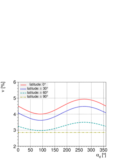
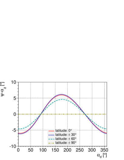
Figure 1: Variations of the $\nu$ (left) and $\psi$ (right) parameters as a function of the dipole phase $\alpha_{d}$ for a dipole amplitude $d=5\%$ in the case of a non-uniform directional exposure, for different latitudes of virtual observatories.

Turning now to the case of a non-uniform directional exposure in right ascension, and considering a general cosmic ray flux $\tilde{\Phi}$ depending on both $\delta$ and $\alpha$, it turns out from equation 28 that the assumption made in sub-sections 2.2 and 2.3, namely that the observed distribution in right ascension is the product between the directional exposure $\omega(\alpha)$ and the function $\Phi(\alpha)$, is in fact not fulfilled if the function $\tilde{\omega}(\delta,\alpha)$ cannot be factorised - and there is no reason that this function could be factorised in practical cases. Formally, this implies that the recovered harmonic coefficients are necessarily biased since genuine anisotropy effects cannot be fully decoupled from exposure effects. Considering for simplicity the estimates defined in sub-section 2.2 only, this can be easily seen from the formal expression of the estimators :

$$\tilde{N} = \int\mathrm{d}\Omega~{}\frac{\tilde{\omega}(\delta,\alpha)}{\omega(\alpha)}~{}\tilde{\Phi}(\delta,\alpha),$$

$$a_{n}^{c} = \frac{2}{\tilde{N}}\int\mathrm{d}\Omega~{}\frac{\tilde{\omega}(\delta,\alpha)}{\omega(\alpha)}~{}\tilde{\Phi}(\delta,\alpha)~{}\cos{n\alpha},$$

$$a_{n}^{s} = \frac{2}{\tilde{N}}\int\mathrm{d}\Omega~{}\frac{\tilde{\omega}(\delta,\alpha)}{\omega(\alpha)}~{}\tilde{\Phi}(\delta,\alpha)~{}\sin{n\alpha},$$ (30)

which, given the definitions of $\omega(\alpha)$ and $\Phi(\alpha)$, cannot be written in the same form as equations 2 (except if $\tilde{\Phi}$ depends only on $\alpha$, which is a very specific case).

We exemplify here that, however, the biases are not large even in a case of a relatively large variation of $\omega(\alpha)$. For $n=1$ for instance, the relationship between the dipole vector $\mathbf{d}$ parameters and the first harmonic parameters $\{\nu,\psi\}$ can be calculated numerically from equations 2.4.2. Some illustrations of this relation are shown in Figure 1 for $d=5\%,\delta_{d}=0^{\circ}$ and different latitudes of virtual observatories fully efficient up to $60^{\circ}$ and with a variation of the detection efficiency with local sidereal time $T$ proportional to $1+0.3\cos{T}$. The time dependence of the detection efficiency translates into a right ascension dependence of the directional exposure, except for observatory latitudes located at the poles of the Earth where the whole range of right ascensions is in the field of view at any time, resulting in a uniform exposure. It can be seen that both $\nu$ and $\psi$ undergo now some variations with the dipole phase $\alpha_{d}$ for a wide range of latitudes, except, as expected, for those located at the poles of the Earth where the distance between $\nu$ and $d$ is, however, the largest. This kind of behaviour will be important to consider for understanding the performances of the shuffling method in sub-section 3.4.

For completeness, we provide also the amplitude and phase p.d.f. expected for non-zero $\nu$. Only semi-analytical expressions can be derived :

$$p_{N}(\overline{r};\nu,\psi) = \frac{\overline{r}}{2\pi\sigma^{c}\sigma^{s}}\exp{\bigg{(}-\frac{\nu^{2}\cos^{2}{\psi}}{2{\sigma^{c}}^{2}}-\frac{\nu^{2}\sin^{2}{\psi}}{2{\sigma^{s}}^{2}}\bigg{)}}\times$$ (31)

$$\displaystyle\int \mathrm{d}\overline{\phi}~{}\exp{\bigg{(}-\frac{\overline{r}^{2}\cos^{2}{\overline{\phi}}}{2{\sigma^{c}}^{2}}-\frac{\overline{r}^{2}\sin^{2}{\overline{\phi}}}{2{\sigma^{s}}^{2}}+\frac{\overline{r}\nu\cos{\psi}\cos{\overline{\phi}}}{{\sigma^{c}}^{2}}+\frac{\overline{r}\nu\sin{\psi}\sin{\overline{\phi}}}{{\sigma^{s}}^{2}}\bigg{)}},$$

$$p_{\Psi}(\overline{\phi};\nu,\psi) = \frac{1}{2\pi\sigma^{c}\sigma^{s}}\exp{\bigg{(}-\frac{\nu^{2}\cos^{2}{\psi}}{2{\sigma^{c}}^{2}}-\frac{\nu^{2}\sin^{2}{\psi}}{2{\sigma^{s}}^{2}}\bigg{)}}\times$$ (32)

$$\displaystyle\int \mathrm{d}\overline{r}~{}\overline{r}\exp{\bigg{(}-\frac{\overline{r}^{2}\cos^{2}{\overline{\phi}}}{2{\sigma^{c}}^{2}}-\frac{\overline{r}^{2}\sin^{2}{\overline{\phi}}}{2{\sigma^{s}}^{2}}+\frac{\overline{r}\nu\cos{\psi}\cos{\overline{\phi}}}{{\sigma^{c}}^{2}}+\frac{\overline{r}\nu\sin{\psi}\sin{\overline{\phi}}}{{\sigma^{s}}^{2}}\bigg{)}}.$$

2.5 Note on the dipolar interpretation of the first harmonic coefficients

The parameters $\nu$ and $\psi$ are often interpreted as indirect estimations of the dipole parameters $d$ and $\alpha_{d}$, based on the relationships established in equations 2.4.1 or 2.4.2. Actually, for a general angular distribution $\tilde{\Phi}(\delta,\alpha)$ with multipolar moments beyond the dipole, these simple relationships do not hold anymore and there is no simple way to relate the first harmonic coefficients to the dipole parameters anymore.

For convenience, this statement is demonstrated here only in the case of a uniform exposure function in right ascension. In its most general form, the flux on the sphere can be decomposed as an infinite sum of spherical harmonics $Y_{\ell m}(\delta,\alpha)$ with multipolar coefficients $a_{\ell m}$. Inserting this expansion into equation 28, the angular distribution $\Phi(\alpha)$ can be expressed as :

$$\Phi(\alpha)\propto\int\mathrm{d}\delta~{}\cos{\delta}~{}\tilde{\omega}(\delta)\bigg{(}1+\sum_{\ell\geq 1}\sum_{m=-\ell}^{\ell}a_{\ell m}Y_{\ell m}(\delta,\alpha)\bigg{)}.$$ (33)

Using the fact that $Y_{\ell m}(\delta,\alpha)$ functions are proportional to the product of the associated Legendre polynomials $P_{\ell m}$ for $\sin{\delta}$ and of harmonic functions for $\alpha$, the explicit dependence of $\Phi(\alpha)$ in $\cos{\alpha}$ and $\sin{\alpha}$ can be written as :

$$\Phi(\alpha) \propto 1+\sum_{\ell\geq 1}\sqrt{\frac{(2\ell+1)(\ell-1)!}{2\pi(\ell+1)!}}\left\langle P_{\ell 1}(\sin{\delta})\right\rangle\bigg{(}a_{\ell 1}\cos{\alpha}+a_{\ell-1}\sin{\alpha}\bigg{)}+...,$$ (34)

with, as in equation 2.4.1, the shortcut notation

$$\left\langle P_{\ell 1}(\sin{\delta})\right\rangle=\frac{\displaystyle\int\mathrm{d}\delta~{}\cos{\delta}~{}\tilde{\omega}(\delta)P_{\ell 1}(\sin{\delta})}{\displaystyle\int\mathrm{d}\delta~{}\cos{\delta}~{}\tilde{\omega}(\delta)}.$$ (35)

By identifying the first harmonic coefficients in equations 3 and 34, the general relationship between $\{\nu,\psi\}$ and the $a_{\ell\pm 1}$ coefficients is now :

$$\nu=\frac{\bigg{[}\bigg{(}\sum_{\ell\geq 1}\sqrt{\frac{(2\ell+1)(\ell-1)!}{2\pi(\ell+1)!}}\left\langle P_{\ell 1}(\sin{\delta})\right\rangle a_{\ell 1}\bigg{)}^{2}+\bigg{(}\sum_{\ell\geq 1}\sqrt{\frac{(2\ell+1)(\ell-1)!}{2\pi(\ell+1)!}}\left\langle P_{\ell 1}(\sin{\delta})\right\rangle a_{\ell-1}\bigg{)}^{2}\bigg{]}^{0.5}}{1+\sum_{\ell\geq 0}\sqrt{\frac{(2\ell+1)}{4\pi}}\left\langle P_{\ell 0}(\sin{\delta})\right\rangle a_{\ell 0}},$$ (36)

$$\tan{\psi}=\frac{\sum_{\ell\geq 1}\sqrt{\frac{(2\ell+1)(\ell-1)!}{(\ell+1)!}}\left\langle P_{\ell 1}(\sin{\delta})\right\rangle a_{\ell-1}}{\sum_{\ell\geq 1}\sqrt{\frac{(2\ell+1)(\ell-1)!}{(\ell+1)!}}\left\langle P_{\ell 1}(\sin{\delta})\right\rangle a_{\ell 1}}.$$ (37)

For an exposure function $\tilde{\omega}$ covering mainly one of the hemisphere of the Earth only, it is thus permissible, for instance, that some families of quadrupoles produce a non-zero first harmonic in right ascension, without any dipole pattern in the underlying angular distribution $\tilde{\Phi}$. Hence, for interpreting any measurement of first harmonic in right ascension in terms of dipole amplitude and phase, the additional assumption that the flux $\tilde{\Phi}$ is a pure dipole is needed.

3 Principle of the shuffling technique for large scale anisotropy searches

3.1 Principle of the shuffling technique

Under the hypothesis of isotropy, any shower detected with particular local coordinates could have arrived with equal probability at any other time of a shower detection. The shuffling technique simply exploits this property, in estimating the directional exposure by averaging the number of arrivals in a given target over a large number of simulation data sets [5]. Each simulation data set is obtained by preserving the actual set of arrival directions in local coordinates, and by randomly sampling times from the actual set of measured ones.

Formally, the principle of this approach is to replace the time integration and the $\cos{\delta}$ integration of the collecting area in equation 2 by the solid angle and time integrations of the observed angular distribution $\mathrm{d}N/\mathrm{d}\Omega$ in local angles $\Omega=(\theta,\varphi)$ pointing to the right ascension $\alpha$ at local sidereal time $T$ and weighted by the observed and normalised event time distribution $1/N\times\mathrm{d}N/\mathrm{d}T$, $N$ being the total number of events :

$$\omega_{sh}(\alpha)=\int\mathrm{d}\Omega\mathrm{d}T\frac{1}{N}~{}\frac{\mathrm{d}N(T)}{\mathrm{d}T}~{}\frac{\mathrm{d}N(\Omega)}{\mathrm{d}\Omega}~{}\delta(\alpha(\theta,\varphi,T)-\alpha).$$ (38)

The argument in the Dirac function guarantees that the direction in celestial coordinates considered throughout the integration of the local angles at local sidereal time $T$ corresponds to the right ascension $\alpha$ :

$$\alpha(\theta,\varphi,T)=T+f(\varphi)~{}\arccos{\left(\frac{\cos{\theta}-\cos{\ell}\cos{\delta}}{\sin{\ell}\sin{\delta}}\right)},$$ (39)

with $f(\varphi)=+1$ if $-\pi/2\leq\varphi\leq\pi/2$ and $f(\varphi)=-1$ otherwise for an azimuth angle $\varphi$ defined relative to the East direction and measured counterclockwise. Integrating over solid angle $\Omega=(\theta,\varphi)$ the angular distribution $\mathrm{d}N/\mathrm{d}\Omega$ results in giving to any celestial direction in the field of view available at any given local sidereal time $T$ an instantaneous exposure in proportion to the event rate in the corresponding direction in local angles. Through the integration over local sidereal time $T$ of the actual variation of the event rate $\mathrm{d}N/\mathrm{d}T$, the distortions of the cosmic ray intensity in celestial coordinates induced by experimental variations of the event rate are then automatically accounted for in the definition of $\omega_{sh}(\alpha)$. In contrast, the modulations in celestial coordinates induced by eventual anisotropies are only partially washed out, because for any given local sidereal time $T$, the event time distribution $\mathrm{d}N/\mathrm{d}T$ is sensitive to the global intensity of cosmic rays but not to the underlying structure in right ascension. Hence, the use of equation 38 provides a relevant estimate of the expected background in searching for large scale anisotropies, though with reduced sensitivity.

The main advantage in adopting equation 38 as the directional exposure instead of the actual one relies on the possibility to carry out the integration using only any observed realisations of the angular distribution $\mathrm{d}N/\mathrm{d}\Omega$ and the event time distribution $\mathrm{d}N/\mathrm{d}T$ :

$$\frac{\mathrm{d}N}{\mathrm{d}\Omega}=\sum_{i=1}^{N}\delta(\Omega,\Omega_{i})=\sum_{i=1}^{N}\delta(\cos{\theta},\cos{\theta_{i}})\delta(\varphi,\varphi_{i}),$$ (40)

$$\frac{\mathrm{d}N}{\mathrm{d}T}=\sum_{i=1}^{N}\delta(T,T_{i}).$$ (41)

Inserting equation 40 and equation 41 into equation 38, it is straightforward to see that the function $\omega_{sh}(\alpha)$ can be sampled by Monte-Carlo in shuffling the observed set of measured times and in preserving the the actual set of arrival directions in local coordinates :

$$\omega_{sh}(\alpha)\simeq\frac{1}{N_{sh}}\sum_{j=1}^{N_{sh}}\sum_{i=1}^{N}~{}\delta(\alpha(\theta_{i},\varphi_{i},T_{\sigma_{j}(i)}),\alpha),$$ (42)

where the subscript $\sigma_{j}(i)$ stands for the random permutation of each element $i$. This estimation is only based on any actual data set.

To illustrate the differences between the actual directional exposure $\omega(\alpha)$ (cf equation 2) and $\omega_{sh}(\alpha)$ as estimated from equation 38, let’s consider a surface array experiment located at an Earth latitude $\ell$, and operating with no variation in time of the detection efficiency so that the actual directional exposure $\omega(\alpha)$ is uniform. For a detection efficiency saturated up to some maximal zenith angle $\theta_{\mathrm{max}}$, and in a virtual situation where an infinite number of events would be detected, a dipolar distribution with amplitude $d$, declination $\delta_{d}$ and right ascension $\alpha_{d}$ would modulate the distributions in local angles very little compared to the case of isotropy [11], so that $\mathrm{d}N(\theta,\varphi)/\mathrm{d}\Omega\propto\cos{\theta}$. On the other hand, expressing $\tilde{\Phi}(\delta,\alpha)$ in terms of local sidereal times and local angles $\{\theta,\varphi\}$, and integrating over $\theta$ and $\varphi$ leads to :

$$\frac{\mathrm{d}N(T)}{\mathrm{d}T}\propto 1+\frac{\displaystyle\int\mathrm{d}\Omega~{}\cos^{2}{\theta}}{\displaystyle\int\mathrm{d}\Omega~{}\cos{\theta}}~{}d~{}\cos{\delta_{d}}~{}\cos{\ell}\cos{(T-\alpha_{d})}.$$ (43)

Meanwhile, still for a pure dipolar distribution, the distribution in right ascension is known from equations 2.4.1 :

$$\frac{\mathrm{d}N(\alpha)}{\mathrm{d}\alpha}\propto\left(1+\frac{\left<\cos{\delta}\right>d_{\perp}}{1+\left<\sin{\delta}\right>d_{\parallel}}~{}\cos{(\alpha-\alpha_{d})}\right),$$ (44)

where $d_{\parallel}=d\sin{\delta_{d}}$ denotes the component of the dipole along the Earth rotation axis while $d_{\perp}=d\cos{\delta_{d}}$ is the component in the equatorial plane. For definiteness, all simulated dipoles are oriented in the equatorial plane in the following. For $\ell=-35^{\circ}$ (as in the case of the Pierre Auger observatory [12]), $d=5\%$, $\delta_{d}=0^{\circ}$ and $\alpha_{d}=0^{\circ}$ for instance, the function $\mathrm{d}N/\mathrm{d}\alpha$ is shown in Figure 2 as the red plain curve. Inserting equation 42 into equation 38, the function $\omega_{sh}(\alpha)$ is shown as the dotted line.

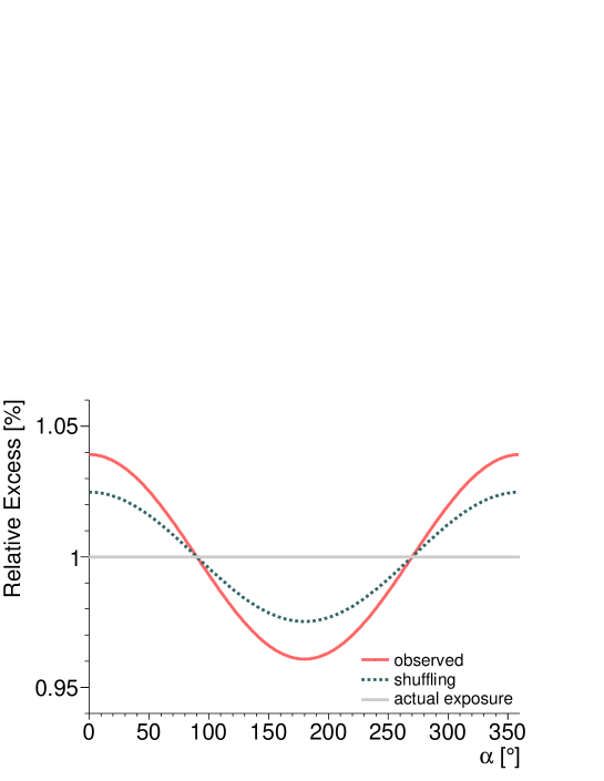
Figure 2: Illustration of the estimation of the directional exposure by means of the shuffling technique (in dotted), compared to the true directional exposure (uniform) and to the observed anisotropy (red plain curve). For convenience, all curves are here re-scaled around 1.

It is visible from Figure 2 that in contrast to $\omega(\alpha)$, $\omega_{sh}(\alpha)$ is not a uniform function : it absorbs part of the modulation introduced in $\mathrm{d}N/\mathrm{d}\alpha$. The anisotropy amplitude estimated by using $\omega_{sh}(\alpha)$ is consequently reduced compared to the one obtained when using the actual directional exposure function $\omega(\alpha)$. This is the reason why the sensitivity to large scale anisotropy searches is expected to be reduced when using the shuffling technique for estimating the directional exposure.

However, due to fluctuation effects related to the finite number of sampled points, the first harmonic of any observed set of $N$ discrete arrival directions is expected to follow equation 44 even for isotropy, with a random phase and an amplitude distributed according to the Rayleigh distribution with parameter $\sigma=\sqrt{2/N}$. Consequently, the non-zero amplitudes resulting from fluctuations effects in the case of isotropy are also expected to be reduced to some extent. Formally, those amplitudes are still expected to follow the Rayleigh distribution but with an effective parameter $\sigma_{\mathrm{sh}}=k\sigma$, with $k$ smaller than 1. This is a crucial mechanism to consider, especially for estimating the significance of any measured amplitude by means of the shuffling technique.

Determining the parameter $k$ in a formal semi-analytical way turns out to be a difficult task. This is because once the fluctuations associated to the finite number of events are considered, any sets of $a_{\ell\pm 1}$ coefficients leading to the same first harmonic for the distribution $\mathrm{d}N/\mathrm{d}\alpha$ (cf sub-section 2.5) impact in a different way $\mathrm{d}N/\mathrm{d}T$. In other words, there is no one-to-one relation between the first harmonic coefficients of $\mathrm{d}N/\mathrm{d}\alpha$ and the ones of $\omega_{sh}(\alpha)$. Hence, we defer to Monte-Carlo simulations to calculate the parameter $k$ in the following, based on a more sensible toy observatory.

3.2 Test of the shuffling technique : a toy observatory

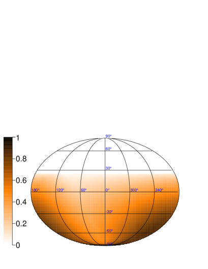
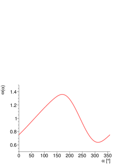
Figure 3: Directional exposure of the toy observatory considered in the Monte-Carlo simulations. Left : dependence on both right ascension and declination, in Mollweide projection. Right : dependence in right ascension only.

To probe the performances of the shuffling technique in searching for large scale anisotropies, we will consider in each following sub-section 1,000 mock samples generated from an isotropic or a dipolar distribution with a total number of events $N=100,000$. The toy observatory considered hereafter is assumed to have a detection efficiency depending on UTC time in such a way that the simulated observatory is operating only 8 hours per solar day, with a seasonal harmonic modulation reaching 4 hours. At the sidereal time scale, this results in a net dipolar modulation of $\simeq 30\%$ of the directional exposure in right ascension, as can be seen in Figure 3. The exposure shown in the right panel will be referred to as the actual exposure in the following. Such a behaviour roughly mimics fluorescence or Cherenkov telescopes.

Without loss of generalities, we restrict ourselves in the following to the first harmonic estimation from a set of $N$ events. This is the most challenging to extract from any data set since experimental effects mainly produce a spurious dipolar modulation, and one of the most interesting for cosmic ray physics at all energies.

3.3 Case of isotropy

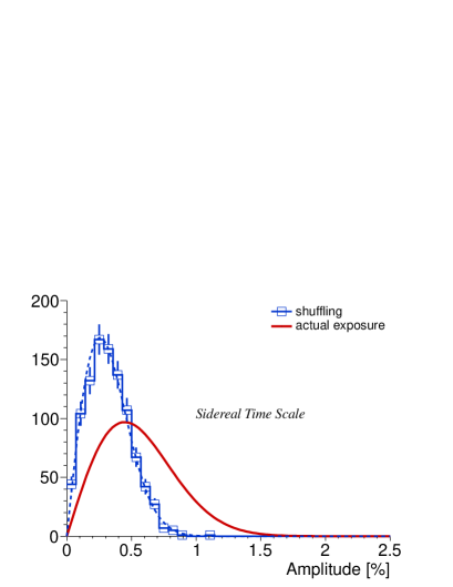
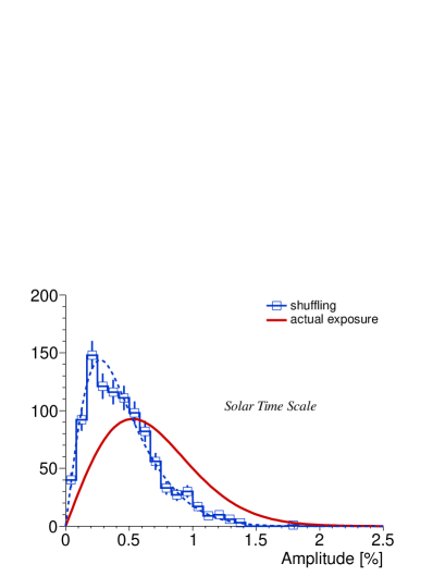
Figure 4: Reconstructed amplitudes for an underlying isotropic distribution, with $N$=100,000 events. Plain curves : Expected distribution of amplitudes from the actual directional exposure. Histograms : Distribution of reconstructed amplitudes with the directional exposure as derived from the shuffling technique. Left panel : sidereal time scale. Right panel : solar time scale.

Generating mock samples drawn from isotropy, the distribution of amplitudes obtained by applying the shuffling procedure on each sample to estimate the directional exposure is shown in the left panel of Figure 4, as the blue histogram. For reference, the distribution that the histogram of reconstructed amplitudes would fit if the actual directional exposure was used is shown as the red curve. Rigorously, this distribution is described in equation 14. However, though the directional exposure is largely non-uniform, the parameters $\sigma_{1}^{c}$ and $\sigma_{1}^{s}$ differ from $\sigma=\sqrt{2/N}$ only slightly : $\sigma_{1}^{c}\simeq 1.02~{}\sigma$ and $\sigma_{1}^{c}\simeq 1.03~{}\sigma$, so that equation 14 is here undistinguishable from a Rayleigh distribution with parameter $\sigma$. As a consequence of the absorption described above, a compression of the reconstructed amplitudes is clearly observed. The histogram can still be fitted by the Rayleigh distribution, but by rescaling the $\sigma$ parameter by a global factor : $\sigma_{\mathrm{sh}}\simeq 0.57\sigma$. The compression is an essential feature to consider when searching for anisotropies, that will be exploited in next sections.

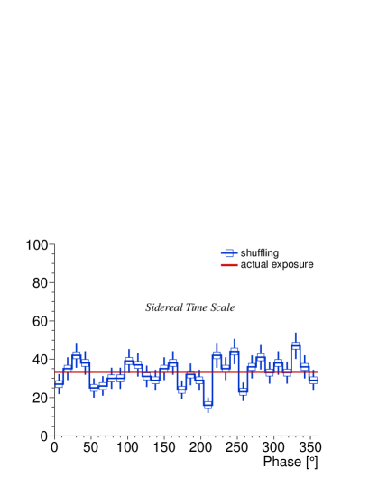
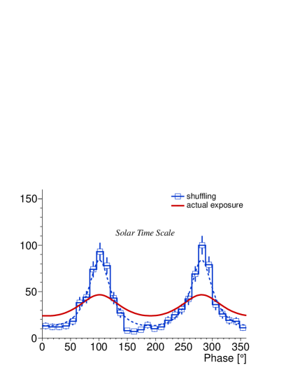
Figure 5: Reconstructed phases for an underlying isotropic distribution, with $N$=100,000 events. Plain curves : Expected distribution of phases from the actual directional exposure. Histograms : Distribution of reconstructed phases with the directional exposure as derived from the shuffling technique. Left panel : sidereal time scale. Right panel : solar time scale.

To provide further illustration, the same simulations are repeated at the solar time scale. Given the time dependence of the efficiency, the net dipolar modulation of the directional exposure is amplified at this particular time scale, reaching almost $100\%$. This is a very significant spurious modulation, requiring us to perform here first harmonic analyses using the formalism presented in sub-section 2.3. The distribution of amplitudes that would be obtained with the actual directional exposure, shown as the red curve in the right panel of Figure 4, is derived from equation 14 with resolution parameters obtained from equation 2.3 : $\sigma_{1}^{c}=1.01\sqrt{2/N}$ and $\sigma_{1}^{s}=1.41\sqrt{2/N}$. In contrast, the distribution of amplitudes obtained by applying the shuffling procedure is shown as the blue histogram. A compression is also observed. As in the previous case, parameters $\sigma_{1,\mathrm{sh}}^{c}$ and $\sigma_{1,\mathrm{sh}}^{s}$ can be empirically determined so that this histogram can be accurately fitted by equation 14 : $\sigma_{1,\mathrm{sh}}^{c}\simeq 0.42\sigma_{1}^{c}$ and $\sigma_{1,\mathrm{sh}}^{s}\simeq 0.77\sigma_{1}^{s}$.

Together with the amplitude, the reconstruction of the phase of the first harmonic is a fundamental piece of information. As outlined above, the parameters $\sigma_{1}^{c}$ and $\sigma_{1}^{s}$ (and consequently $\sigma_{1,\mathrm{sh}}^{c}$ and $\sigma_{1,\mathrm{sh}}^{s}$) are, at the sidereal time scale, too close each other to induce notable differences between equation 15 and a uniform function. The distribution of phases is thus expected to be uniform to a high level even when using the shuffling technique. This is observed to be the case, as shown in the left panel of Figure 5. On the other hand, at the solar time scale, the distribution of phases is expected to follow equation 15, with the same $\sigma_{1,\mathrm{sh}}^{c}$ and $\sigma_{1,\mathrm{sh}}^{s}$ parameters as the ones derived empirically for the distribution of amplitudes. This is indeed the case, as shown in the right panel of Figure 5 by the dotted curve matching the histogram. The distribution that would be obtained using the actual directional exposure is shown as the continuous curve. This latter curve is flatter and so closer to a uniform distribution, which is a first illustration of the loss of sensitivity when using the shuffling technique - though in an extreme case. This loss of sensitivity will be exemplified and quantified farther.

3.4 Case of anisotropy

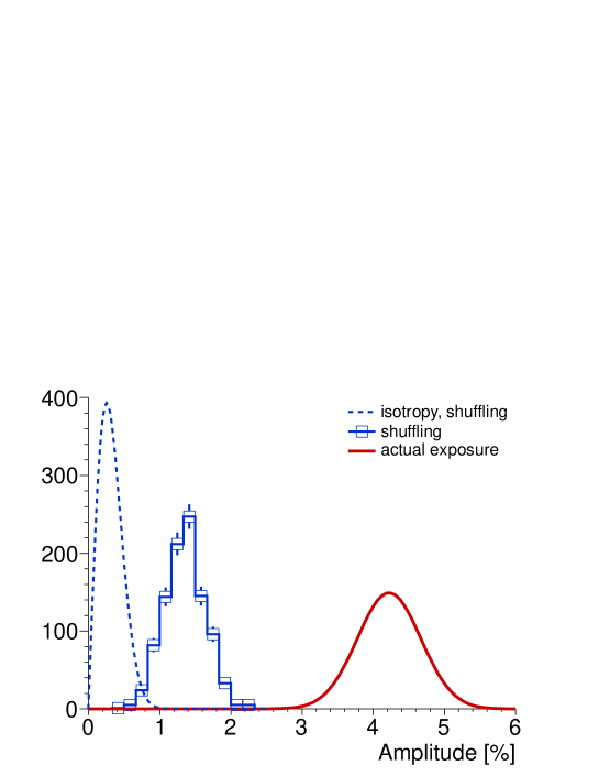
Figure 6: Reconstructed amplitudes for an underlying dipolar distribution with amplitude $d_{\perp}=5\%$ and $N$=100,000 events. Histogram : Distribution of reconstructed amplitudes with the directional exposure as derived from the shuffling technique. Plain curve : Expected distribution of amplitudes when using the true directional exposure. Dotted curve : Distribution of amplitudes for isotropy, as empirically reconstructed from the shuffled event sets built with the directional exposure as derived from each simulated sample.

We consider now dipolar distributions of cosmic rays, at the sidereal time scale only. By analogy with the isotropic case, there are no notable differences between equations 26-27 and equations 31 due to the closeness between $\sigma_{1}^{c}$ and $\sigma_{1}^{s}$ so that, for simplicity, we use equations 26-27 in the following discussion, with $\sigma=\sqrt{2/N}$. For a dipole amplitude $d_{\perp}=5\%$, and with the actual directional exposure, the parameters $\nu$ and $\psi$ entering into equations 26-27 are given from the set of coefficients in equation 2.4.2. Their variation with the actual dipole phase $\alpha_{d}$ is almost the same as the illustration depicted in Figure 1 for the observatory latitude at $\pm 30^{\circ}$. Given the toy observatory considered in the simulations, for $d_{\perp}=5\%$ and $\alpha_{d}=0^{\circ}$ for instance, the expectation for $\nu$ is $\simeq 4.2\%$ . The corresponding distribution of reconstructed amplitudes is shown as the plain red curve in Figure 6. On the other hand, the distribution of reconstructed amplitudes with the directional exposure as derived from the shuffling technique is shown as the blue histogram. This histogram can be fitted by equation 26 by rescaling the $\sigma$ parameter in the same way as in the case of isotropy (i.e. $\sigma_{\mathrm{sh}}\simeq 0.57\sigma$) and with a $\nu$ parameter such that $\nu_{\mathrm{sh}}=1.32\%\pm 0.01\%$ instead of $\nu=4.2\%$. Though part of the anisotropy signal is, as expected, absorbed, it can be seen however that significant amplitudes can be discerned by comparison of the blue histogram in Figure 6 with the one in Figure 4.

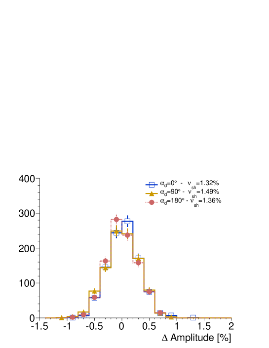
Figure 7: Reconstructed amplitudes centered on the expected $\nu_{\mathrm{sh}}$ parameter for an underlying dipolar distribution with amplitude $d_{\perp}=5\%$, $N$=100,000 events, and different dipole phases $\alpha_{d}$. The directional exposure is derived from the shuffling technique.

Though this is irrelevant in practice since $\tilde{\omega}(\delta,\alpha)$ is by construction not accessible to knowledge when using the shuffling technique, it is anyway interesting to check here that the resulting value for $\nu_{\mathrm{sh}}$ is in agreement with the one that can be derived from equations 2.4.2 when inserting the numerical values of $\omega_{\mathrm{sh}}$ averaged over many realisations in the denominators of these equations. This turns out to be the case, as illustrated in Figure 7, where the expected $\nu_{\mathrm{sh}}$ is subtracted to the reconstructed amplitudes for several values of dipole phases $\alpha_{d}$. All histograms can be observed to be centered on zero.

Hence, from any single mock sample, it appears interesting to aim at reconstructing in an empirical way a relevant distribution of amplitudes that would have been obtained with an underlying isotropic angular distribution of cosmic rays. This can be done using the following recipe :

1. From any given data set, the directional exposure is obtained by means of the shuffling technique, allowing an amplitude $\overline{r}_{1}^{obs}$ to be inferred.

2. New mock samples are then generated, still by means of the shuffling technique.

3. The shuffling procedure is applied to each mock sample generated in step 2, allowing the directional exposure of each mock sample to be known. The corresponding distribution of amplitudes $\overline{r}_{1}$ is then constructed in an empirical way.

4. The amplitude $\overline{r}_{1}^{obs}$ is then compared to the empirical distribution obtained in step 3.

The result of this procedure is shown in Figure 6 too, as the blue dotted curve. Here, for clarity, what is shown is not the histogram obtained for any realisation but the corresponding fit using equation 14. It turns out that the distribution of amplitudes obtained in that way is in agreement with the one obtained in previous sub-section 3.3 for isotropy. In other words, the procedure described above provides a distribution of amplitudes that makes it possible to estimate the significance of any measured amplitude obtained with a directional exposure estimated by means of the shuffling technique. This procedure is only based on any given data set.

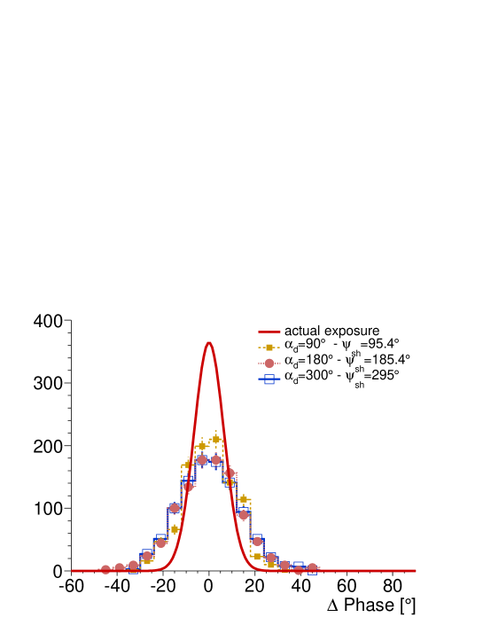
Figure 8: Reconstructed phases for an underlying dipolar distribution with amplitude $d_{\perp}=5\%$ and $N$=100,000 events. Histograms : Distribution of reconstructed phases with the directional exposure as derived from the shuffling technique, and for three directions of the dipole phase. Plain curve : Expected distribution of phases when using the actual directional exposure.

For completeness, the distributions of reconstructed phases are shown as the histograms in Figure 8, after subtraction of the expected $\psi$ and $\psi_{\mathrm{sh}}$ for both the actual exposure $\omega(\alpha)$ and the shuffling one $\omega_{\mathrm{sh}}(\alpha)$ respectively. The distribution that would be obtained using the actual directional exposure is shown again as the red plain curve. On the other hand, the reconstructed distributions using the shuffling technique are shown as the blue histograms for three directions of the dipole phase : one along the direction of maximum of exposure $\alpha_{d}=180^{\circ}$, a second one in the direction of minimum of exposure $\alpha_{d}=300^{\circ}$, and a third one in the direction $\alpha_{d}=90^{\circ}$. All distributions are centered and can be fitted by equation 27 with the same parameters $\sigma_{\mathrm{sh}}$ and $\nu_{\mathrm{sh}}$ as the ones derived from Figure 6. The resulting width of these curves is larger than the one that would be obtained in the ideal case, which is a new illustration of the loss of sensitivity when using the shuffling technique, loss of sensitivity that we quantify in next section.

It is important to stress that, in the light of results obtained in section 2.4, the parameters $\nu_{\mathrm{sh}}$ and $\psi_{\mathrm{sh}}$ are related to the dipole parameters $d_{\perp}$ and $\alpha_{d}$ in an inaccessible way in the case of a non-uniform directional exposure in right ascension since the directional exposure function $\tilde{\omega}(\delta,\alpha)$ is supposed to be unknown in the practical cases where the shuffling technique is relevant. In practice, the only possible way to convert $\nu_{\mathrm{sh}}$ and $\psi_{\mathrm{sh}}$ into $d_{\perp}$ and $\alpha_{d}$ thus requires the use of equation 2.4.1 (that is, ignoring the non-uniformities of the directional exposure in right ascension). This approximation leads unavoidably to small biases for the estimation of $d_{\perp}$ and $\alpha_{d}$.

4 Performances of the shuffling technique for large scale anisotropy searches

4.1 Detection power

The performances of the procedure described in previous section in searching for real anisotropies are presented in this section. They are given in terms of detection power at some threshold value. The threshold - or type-I error rate - is the fraction of isotropic simulations in which the null hypothesis is wrongly rejected (i.e. the test provides evidence of anisotropy when there is no anisotropy). On the other hand, the detection power, defined as $1-\beta$ with $\beta$ the type-II error rate, provides the fraction of anisotropic simulations in which the null hypothesis is (correctly) rejected.

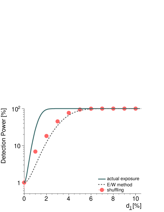
Figure 9: Detection power for dipolar anisotropy searches as a function of $d_{\perp}$. The threshold is fixed at 1%. The results obtained using the shuffling (red points) are compared to the ones obtained with the actual exposure (plain curve) and with the East/West method (dotted curve).

Still with mock samples with a total number of events $N=100,000$ and in the same conditions of detection efficiency as in sub-section 3.4, the detection power is shown in Figure 9 as a function of $d_{\perp}$, and for random phases $\alpha_{d}$. The threshold is fixed here at 1%. The results obtained using the shuffling (red points) are compared to the ones obtained with the actual exposure (plain curve). For illustration, the results obtained using the East/West method [13] are also shown as the dotted curve. This method is based on the analysis of the difference of the counting rates in the eastward and the westward directions, and is largely independent of experimental effects without requiring corrections for directional exposure and/or atmospheric effects. To maximise the performances of the East/West method, our simulated observatory is assumed to present a perfect symmetry to eastward and westward directions. Though the detection power is saturated much earlier in the case of the first harmonic analysis using the actual directional exposure, it turns out that the procedure described in sub-section 3.4 performs slightly better than the East/West method. In addition, it is worth noting that the procedure presented here potentially pertains to any type of detector (i.e. even for fluorescence or Cherenkov telescopes).

4.2 From the measured amplitude to $d_{\perp}$

At this stage, the procedure presented above provides a relevant framework to reveal large scale anisotropy. However, for cosmic ray physics, it is interesting not only to detect anisotropy but also to estimate $d_{\perp}$. This task is straightforward to achieve when the actual directional exposure is known and when a pure dipole is assumed by means of equation 44. This is illustrated by the dotted blue line in Figure 10. For convenience, the amplitude range that can be obtained in 99% of isotropic fluctuations is delimited by the orange area.

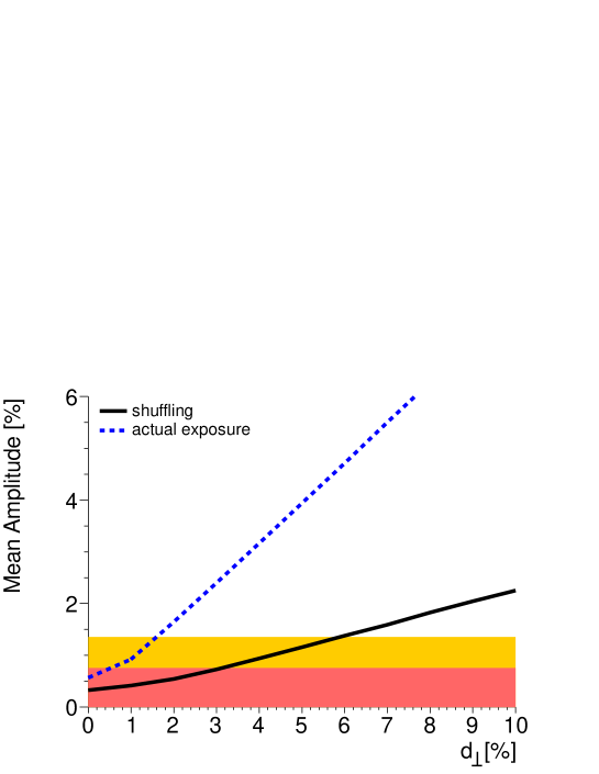
Figure 10: Mean amplitude of the first harmonic as a function of $d_{\perp}$.

In contrast, when using the shuffling technique to get at the exposure, equation 44 does not hold any longer. To estimate the conversion curve between $\left<r\right>$ and $d_{\perp}$, the procedure described in sub-section 3.4 can be applied by replacing the second step in this way : New mock samples are then generated, still by means of the shuffling technique. In addition, each event is accepted or rejected by randomly sampling its right ascension according to the modulation in right ascension induced by a dipole with amplitude $d_{\perp}$ and phase $\alpha_{d}$. The resulting curve obtained in the same simulated experimental conditions as previously is shown as the black curve in Figure 10, together with the amplitude range that can be obtained in 99% of isotropic fluctuations (red area). This curve allows a calibration of the measured amplitude in terms of $d_{\perp}$. For instance, a measured amplitude $\overline{r}^{obs}=1\%$, providing evidence for anisotropy at more than 99% confidence level, corresponds in fact to $d_{\perp}=4\%$ in this specific example.

5 Conclusions

The shuffling technique has been studied to search for large scale anisotropies of cosmic rays. Accounting for the compression of the reconstructed amplitude distribution in the case of an underlying isotropic distribution, it has been shown that this technique can be used to reveal dipolar patterns though with reduced sensitivity compared to the one that would be obtained with the perfect knowledge of the actual directional exposure. In spite of this reduced sensitivity, the gain of this method relies on avoiding any corrections for the observed counting rates. This holds for any surface array detectors, fluorescence telescopes, and/or Cherenkov telescopes.

References

- [1] J. Linsley, Phys. Rev. Lett. 34 (1975) 1530
- [2] J. Lloyd-Evans, PhD thesis, University of Leeds, 1982
- [3] The Pierre Auger Collaboration, Astropart. Phys. 32 (2009) 89
- [4] F. J. M. Farley, J. R. Storey, Proc. Phys. Soc. A, 67 (1954) 996
- [5] G. L. Cassiday et al., Phys. Rev. Lett. 62 (1989) 383
- [6] D. E. Alexandreas et al., NIM A 328 (1993) 570
- [7] B. Rouillé d’Orfeuil, PhD thesis, Université Paris \@slowromancapvii@, 2007
- [8] E. M. Santos et al., Astropart. Phys. 30 (2008) 39
- [9] S. Mollerach, E. Roulet, JCAP 0508 (2005) 004
- [10] J. Aublin, E. Parizot, Astron. and Astrophys. 441 (2005) 407
- [11] The Pierre Auger Collaboration, ApJS 203 (2012) 34
- [12] The Pierre Auger collaboration, NIM A 523 (2004) 50
- [13] R. Bonino et al., ApJ 738 (2011) 67