Quantum simulations of the early universe

Abstract

A procedure is described whereby a linearly coupled spinor Bose condensate can be used as a physically accessible quantum simulator of the early universe. In particular, an experiment to generate an analog of an unstable vacuum in a relativistic scalar field theory is proposed. This is related to quantum theories of the inflationary phase of the early universe. There is an unstable vacuum sector whose dynamics correspond to the quantum sine-Gordon equations in one, two or three space dimensions. Numerical simulations of the expected behavior are reported using a truncated Wigner phase-space method, giving evidence for the dynamical formation of complex spatial clusters. Preliminary results showing the dependence on coupling strength, condensate size and dimensionality are obtained.

I Introduction

The use of quantum simulation as a route to better understanding of complex quantum dynamics has much to recommend it. Conceptually, this creates an analog quantum computer. In quantum simulations, a table-top experiment is carried out to mimic a more complex quantum system which we would like to understand. This method has been used to treat, for example, models of condensed matter phase-transitions Porras and Cirac (2004). Such an approach can be complemented by the use of approximate computer simulations. A numerical simulation can then be verified and tested in the table-top experiment, while allowing a wider variety of parameters to be treated.

But why stop at condensed matter: why not model the entire universe? This seems presumptuous, and possibly is. The entire universe will never be shoehorned into a table-top experiment with every complexity intact. Nevertheless, cosmologists today often use quantum field theory models to describe the early universe. This can be traced back to the pioneering works of Higgs and colleagues Higgs (1964a); Englert and Brout (1964); Higgs (1964b); Guralnik et al. (1964), studying the origins of mass, and to Coleman’s groundbreaking studies on unstable quantum vacuum decay Coleman (1977); Callan and Coleman (1977).

A combination of these approaches, together with the inclusion of general relativity, leads to the current inflationary universe scenario Guth (1981); Linde (1991, 1994, 1998); Stewart and Lyth (1993); Liddle et al. (1994). Inflation provides a possible explanation for the origin of structure in the universe. Can we model at least part of this picture of the early universe in a laboratory? The simplest model for the scalar inflaton field $\phi(x)$ is described by the Lagrangian

$${\cal L}=\frac{1}{2}\partial_{\mu}\phi\partial^{\mu}\phi-V(\phi),$$ (1)

where $V(\phi)$ is the potential down which the scalar field rolls or decays. In this paper, we show how to realize the above relativistic scalar field model in a coupled Bose condensate, and model the fate of the scalar field of the early universe. We note that there have been earlier proposals using somewhat different, albeit related techniques Fischer and Schützhold (2004); Neuenhahn et al. (2012).

While the potential $V(\phi)$ is specific, depending on the model of inflation under consideration, coupled Bose condensates provide a situation with $V(\phi)\propto-\cos(\phi)$. In the spirit of inflation, we consider a cold, unstable vacuum with $\phi=\pi$ as the initial condition. The vacuum gradually decays Linde (1991, 1994, 1998), to produce a hot universe, replete with dynamical clumping into random structures. This quantum dynamical “universe on a table-top” experiment is probed by means of an internal Rabi rotation, and imaged.

Relativistic quantum field theory is usually tested experimentally at large accelerators. However, energies at high energy particle accelerators like CERN are not high enough for these field theories, although observational evidence for the Higgs boson ATLAS Collaboration (2012); CMS Collaboration (2012) is thought to provide evidence for the low energy sector of scalar quantum fields in the universe. Instead of accelerating particles to light speed, we propose, essentially, to slow the velocity of light down to atomic speeds. This allows us to study novel phenomena outside of CERN’s limits. A quantum simulation of interacting relativistic fields in two, three or four space-time dimensions has the useful feature that it allows us to access quantum physics that we cannot do experiments on by any other means.

We note some recent experiments have explored relevant physics with ultra-cold atoms, demonstrating that our proposal is indeed feasible. These show that the physics of interest here is very close to realization. The investigations that are similar to our proposal include long time-scale interferometry with a two-level BEC Egorov et al. (2011), and the study of the thermalization of a BEC Gring et al. (2012). More recent experiments have realized a flat trap or “can” for a BEC in three dimensions Gaunt et al. (2013). In principle, simulations of this type might eventually produce results that can predict the early universe temperature maps Planck Collaboration (2013) produced recently by the Planck telescope surveys, or very large-scale density inhomogeneities. Here we have a more cautious goal, of simply being able to demonstrate quantum simulations of an unstable quantum vacuum in a relativistic quantum field theory.

Our starting point is a trapped Bose condensate with two internal quantum levels. The levels are coupled by a microwave field, and the atoms interact through S-wave scattering. We assume zero temperatures, homogeneous couplings and perfect microwave phase stability. While departures from such perfection can be treated, and these requirements can be relaxed, we will study the ideal case here. We show that by introducing a simple $\pi$ phase shift into the coupling field, it is possible to generate an experimentally accessible model of an unstable relativistic vacuum. A quantum simulation of the decay of this unstable vacuum then provides the simplest of early universe models. The relevant field variable is the relative phase of the two condensates. In a regime of small coupling, the relative phase obeys the sine-Gordon equation Kaurov and Kuklov (2006); Gritsev et al. (2007), a popular model for a relativistic scalar field theory where the field potential $V(\phi)$ is a cosine.

This paper demonstrates the feasibility of a class of experiments which can simulate fundamental aspects of models of inflation. Such experiments, as well as theoretical calculations and numerical simulation, should follow a step-by-step programme that starts with the simplest possible theories. In the early stages, naturally, one will learn a lot about how to extract meaningful data from experiments and the adequacy of approximate numerical techniques but not much about the universe. Here we illustrate our approach by a numerical simulation of quantum effects, using a truncated Wigner approximation described later. The results show the importance of a hybrid approach, combining numerical and experimental techniques. Each method involves different physical approximations. By comparing them, one can hope to come to an improved understanding of how quantum fluctuations behave in the nonlinear regime, where exact quantum field predictions are hard to come by. As the programme is extended to include additional quantum fields and the effects of gravity one can hope to connect the results of experiments with astronomical observations and refine our models of the universe.

In general, the longer term fate of vacuum fluctuations in the nonlinear regime is of great fundamental interest. It is not known how to calculate this exactly, due to quantum complexity and the failure of perturbation theory. We speculate that these nonlinear effects may be related to very large scale inhomogeneities in the mass distribution of the universe. This in turn could provide the basis for observational tests of inflationary universe theories beyond those available now. Unlike some modern models of inflation Linde (1991, 1994, 1998), our system can support domain walls of relative phase Son and Stephanov (2002). For experimental studies, these provide an easily measured signature of vacuum decay, and may have cosmological implications.

The paper is organized as follows. In Section (II) we describe the general theory of coupled Bose fields, as found in Bose-Einstein condensate (BEC) experiments on ultra-cold atomic gases at nanoKelvin temperatures. In Section (III), we treat the different types of classical vacuum that exist, and the density-phase representation. In Section (IV) we transform to the sine-Gordon Lagrangian, and demonstrate how this can behave as a relativistic field theory with an unstable vacuum. In Section (V) we carry out detailed, though approximate, numerical simulations of the original field theory, to indicate what to expect in an experiment. Finally, in Section (VI) we discuss the conclusions.

II Coupled Bose fields

Our first task then, is to slow down light: to a few centimeters per second if possible. How is this to be achieved? For the purpose, we use quasi-particles with dispersion relations equivalent to relativistic equations, in a coupled ultra-cold Bose condensate (BEC). To understand this, let us consider the dynamical equations for a coupled condensate; a $D$-dimensional Bose gas with two spin components that are linearly coupled by an external microwave field. This system obeys the following non-relativistic Heisenberg equation:

$$i\hbar\partial_{t}\Psi_{1} = \left\{-\frac{\hbar^{2}}{2m}\nabla_{x}^{2}+g_{1}\Psi_{1}^{\dagger}\Psi_{1}+g_{c}\Psi_{2}^{\dagger}\Psi_{2}\right\}\Psi_{1}-\nu\Psi_{2},$$

$$i\hbar\partial_{t}\Psi_{2} = \left\{-\frac{\hbar^{2}}{2m}\nabla_{x}^{2}+g_{2}\Psi_{2}^{\dagger}\Psi_{2}+g_{c}\Psi_{1}^{\dagger}\Psi_{1}\right\}\Psi_{2}-\nu\Psi_{1}.$$ (2)

Here, $\nabla_{x}^{2}$ represents the $D$-dimensional Laplacian operator, and $g_{1}$, $g_{c}$ are the $D-$dimensional coupling constants, which are assumed positive. These have known relations with the measured scattering length. The coupling-constant is renormalizable at large momentum cutoff, although our simulations are in the regime of low momentum cutoff, which makes renormalization unnecessary. The field commutators are:

$$\left[\Psi_{1}\left(\mathbf{x}\right),\Psi_{1}^{\dagger}\left(\mathbf{x}^{\prime}\right)\right]=\delta^{D}\left(\mathbf{x}-\mathbf{x}^{\prime}\right)$$ (3)

We use spinor notation, introducing $\bm{\Psi}=(\Psi_{1},\Psi_{2})^{T}$ and write the energy functional as $W=\int d^{D}x\,w$, where the energy density $w(\mathbf{x})$ is

$$w={} \frac{\hbar^{2}}{2m}\nabla_{x}\bm{\Psi}^{{\dagger}}\cdot\nabla_{x}\bm{\Psi}-\nu\bm{\Psi}^{{\dagger}}\sigma_{x}\bm{\Psi}+\frac{g_{s}}{2}:(\bm{\Psi}^{{\dagger}}\bm{\Psi})^{2}:+$$

$$+\frac{g_{sa}}{2}:(\bm{\Psi}^{{\dagger}}{\sigma_{z}}\bm{\Psi})^{2}:+{g_{a}}:(\bm{\Psi}^{{\dagger}}\bm{\Psi})(\bm{\Psi}^{{\dagger}}{\sigma_{z}}\bm{\Psi}):.$$ (4)

Here we have defined $2g_{s}=\frac{1}{2}(g_{1}+g_{2})+g_{c}$, $4g_{a}=g_{1}-g_{2}$, and $2g_{sa}=\frac{1}{2}(g_{1}+g_{2})-g_{c}$. From now on, for simplicity we will assume the case of symmetric self coupling $g_{1}=g_{2}\equiv g$ , so that $g_{a}=0$. In the case where $g_{c}=g$, we further find $g_{sa}=0$. It is important for our purposes that the cross-term $g_{c}$ have a different strength to the self-term $g_{i}$. This is generally achievable in ultra-cold atomic physics, depending on the atomic species and particular Feshbach resonance used for magnetically tunable cases. The fully symmetric case with $g_{c}=g$ is less interesting, and we will assume that $g_{c}=0$ for definiteness in later numerical examples.

We recover the Heisenberg equation from $i\partial_{t}\psi_{i}=\delta W/\delta\psi_{i}^{*}$. Alternatively, we will also recover these equations from a stationary action principle $\delta S=0$ with

$$S=\int dt\,d^{D}x\,[\mathcal{R}\{\bm{\Psi}^{{\dagger}}i\hbar\partial_{t}\bm{\Psi}\}-w] =\int dt\,d^{D}x\,\left[\mathcal{L}_{B}-w\right].$$ (5)

The coupling field $\nu$ is supplied by an external microwave source, and couples the hyperfine levels in the atomic condensate together. In experimental realizations Egorov et al. (2011), this has an adjustable amplitude and phase, good homogeneity, and a long coherence time.

Before proceeding further, we rescale the equations into natural units. The time and distance scale is chosen so that mean-field frequency shifts are of order unity, as are the corresponding Laplacian terms. For typical atomic densities per Bose field of $n=N/V$, where $N$ is the particle number of a given species, and $V$ the volume, this leads to the choice $\tau=t/t_{0}$, and $\bm{\zeta}=\mathbf{x}/x_{0}$, where:

$$t_{0} =\hbar/gn$$

$$x_{0} =\hbar/\sqrt{gnm}\,.$$ (6)

Scaling the fields so that they correspond to densities in the new fields, i.e. $\psi=\Psi x_{0}^{D/2}$, the resulting dimensionless field equations in the symmetric case are

$$i\partial_{\tau}\psi_{1} =\left\{-\frac{1}{2}{\nabla}^{2}+\gamma\psi_{1}^{\dagger}\psi_{1}+\gamma_{c}\psi_{2}^{\dagger}\psi_{2}\right\}\psi_{1}-\tilde{\nu}\psi_{2},$$

$$i\partial_{\tau}\psi_{2} =\left\{-\frac{1}{2}{\nabla}^{2}+\gamma\psi_{1}^{\dagger}\psi_{2}+\gamma_{c}\psi_{1}^{\dagger}\psi_{1}\right\}\psi_{2}-\tilde{\nu}\psi_{1}.$$ (7)

Here, $\nabla$ represents derivatives with respect to $\bm{\zeta}$, $\gamma=1/(nx_{0}^{D})$, $\gamma_{c}=g_{c}/(gnx_{0}^{D})$, and $\tilde{\nu}=\nu/(gn)$. The dimensionless field commutators are:

$$\left[\psi_{1}\left(\bm{\zeta}\right),\psi_{1}^{\dagger}\left(\mathbf{\bm{\zeta}}^{\prime}\right)\right]=\delta^{D}\left(\mathbf{\bm{\zeta}}-\mathbf{\bm{\zeta}}^{\prime}\right).$$ (8)

In one dimension, $\gamma^{2}=\gamma_{LL}\equiv mg/(\hbar^{2}n)$, which is the famous Lieb-Liniger parameter Lieb and Liniger (1963) of the one-dimensional quantum Bose gas.

III Stable and unstable vacua

We now consider a semi-classical approach. We define $\tilde{\psi}_{1}$ as a classical mean field, and we linearize around the classical equilibrium solutions. Vacuum solutions with constant fields, apart from an oscillating phase, are easily found from Eq. (7) as $\tilde{\psi}_{1}^{0}=\sqrt{\tilde{n}}=\pm\tilde{\psi}_{2}^{0}$. An overall phase is chosen to make $\tilde{\psi}_{1}^{0}$ positive and $\tilde{n}=nx_{0}^{D}$ is the dimensionless density. The different signs of $\tilde{\psi}_{2}^{0}$ correspond to two inequivalent vacua. In order to study their stability properties and elementary excitations, we investigate small oscillations around the vacuum solutions. This generalizes the analysis presented in Ref. Brand et al. (2010) to include the cross-coupling with $\gamma_{c}$.

III.1 Linearized solutions

Writing $\tilde{\psi}_{j}=[\tilde{\psi}_{j}^{0}+(u_{k}^{j}e^{i(\tilde{\mathbf{k}}\bm{\zeta}-\tilde{\omega}\tau)}+v_{k}^{j\ast}e^{-i(\tilde{\mathbf{k}}\bm{\zeta}-\tilde{\omega}\tau)})]e^{-i\tilde{{\color[rgb]{1,0,0}{\normalcolor\mu}}}\tau}$, where $\tilde{\mu}$ is the vacuum chemical potential, substituting into Eq. (7) and keeping linear terms we obtain the secular equation $\det[B-\tilde{\omega}]=0$ with

$$B=\left(\begin{array}[]{cccc}H_{0}&\gamma\tilde{n}&\mp\tilde{\nu}+\gamma_{c}\tilde{n}&\gamma_{c}\tilde{n}\\ -\gamma\tilde{n}&-H_{0}&-\gamma_{c}\tilde{n}&\pm\tilde{\nu}-\gamma_{c}\tilde{n}\\ \mp\tilde{\nu}+\gamma_{c}\tilde{n}&\gamma_{c}\tilde{n}&H_{0}&\gamma\tilde{n}\\ -\gamma_{c}\tilde{n}&\pm\tilde{\nu}-\gamma_{c}\tilde{n}&-\gamma\tilde{n}&-H_{0}\end{array}\right),$$ (13)

where $H_{0}=-\frac{1}{2}\tilde{k}^{2}+(2\gamma+\gamma_{c})\tilde{n}-\tilde{\mu}$ and consistency demands that $2\gamma_{s}\tilde{n}=\tilde{\mu}\pm\tilde{\nu}$, where we define $2\gamma_{s}=\gamma+\gamma_{c}$. The sign "+" corresponds to the in-phase and "-" corresponds to the out-of-phase vacua. We find two independent solution branches of the secular equation. The first one is gapless

$$\tilde{\omega}_{1}=\sqrt{\frac{1}{2}\tilde{k}^{2}\left(\frac{1}{2}\tilde{k}^{2}+4\gamma_{s}\tilde{n}\right)},$$ (14)

with eigenvector $\sim(1,-1,1,-1)^{{\rm T}}$ for small $k$, which corresponds to the phase fluctuations of the fields $\delta\arg\tilde{\psi}_{1}=\delta\arg\tilde{\psi}_{2}\propto\sin(\tilde{\mathbf{k}}\bm{\zeta}-\tilde{\omega_{1}}\tau)$. This leads to a sound wave with sound speed $\tilde{v}_{\mathrm{Bog}}=\sqrt{2\gamma_{s}\tilde{n}}$. Solutions with real frequencies indicate stable, propagating waves of small amplitude, whereas imaginary roots indicate an instability. Excitations along this branch are always stable when $2\gamma_{s}\equiv\gamma+\gamma_{c}>0$.

The other branch is gapped, since

$$\tilde{\omega}_{2}=\sqrt{\left(\frac{1}{2}\tilde{k}^{2}\pm 2\tilde{\nu}\right)\left(\frac{1}{2}\tilde{k}^{2}+4\gamma_{sa}\tilde{n}+2\tilde{\nu}\right)},$$ (15)

where $2\gamma_{sa}=\gamma-\gamma_{c}$. The nonlinearity parameter in this second branch differs from the first branch and can be tuned independently due to the presence of the cross-coupling $\gamma_{c}$. The eigenvector corresponding to $\omega_{2}$ is $\sim(1,-1,-1,1)^{{\rm T}}$ for small $k$ and $\nu$, which corresponds to an excitation of relative phase fluctuations of the fields $\delta\arg\tilde{\psi}_{1}=-\delta\arg\tilde{\psi}_{2}\propto\sin(\tilde{\mathbf{k}}\bm{\zeta}-\tilde{\omega}_{2}\tau)$. It is interesting to note that the two branches are decoupled in the linear approximation. We will be particularly concerned with the relative phase dynamics, which has characteristic properties of the elementary excitations of a relativistic field theory. Indeed, expanding to second order in $\tilde{k}$ we may write $\tilde{\omega}_{2}^{2}=\tilde{k}^{2}\tilde{c}_{2}^{2}+\tilde{m}_{2}^{2}\tilde{c}_{2}^{4}$, which is a relativistic dispersion relation with a light speed of $\tilde{c}_{2}^{2}=2\gamma_{sa}\tilde{n}\pm 2\tilde{\nu}$ and rest energy $\tilde{m}_{2}^{2}\tilde{c}_{2}^{4}=4\tilde{\nu}(2\gamma_{sa}\tilde{n}\pm\tilde{\nu})$. The relative phase dynamics will analyzed be more rigorously in the next section.

The second branch also supports unstable modes and governs the dynamics of the unstable vacuum. We are particularly interested in the situation where both $\gamma_{s}$ and $\gamma_{sa}$ are positive. In this case the second branch becomes unstable if the linear coupling is such that $\pm\tilde{\nu}<0$, with the unstable modes satisfying $-4\gamma_{sa}\tilde{n}\mp 2\tilde{\nu}<\tilde{k}^{2}/2<\mp 2\tilde{\nu}$. This occurs either with the fields having the same sign and $\tilde{\nu}<0$, or with the fields having the opposite sign and $\tilde{\nu}>0$.

Thus, in a sufficiently large system where $k$ is continuous, one of the two possible vacua is stable and the other one unstable. The classical field dynamics resulting from the unstable vacuum has been discussed for some special cases in Refs. Lesanovsky and von Klitzing (2007); Montgomery et al. (2010) (see also Ref. Brand et al. (2010)). In this paper we are going to simulate the decay from the unstable vacuum due to quantum fluctuations. The characteristic length scale of the decay modes is larger than $\pi/\sqrt{\left|\tilde{\nu}\right|}$, which will become the largest length scale in the system in the interesting regime where $|\tilde{\nu}|$ is small. The time scales of the unstable mode become large in the sine-Gordon regime. This is compatible with the following inflation requirement: When the scalar field rolls down the potential hill very slowly compared to the expansion of the universe, inflation occurs.

III.2 Density-phase representation

We will continue to consider these equations as classical, or mean-field equations. We use this procedure to give us a better understanding of how the dynamics can be reduced to those of a relativistic scalar field. Once we have made this transformation, we will use Lagrangian quantization methods to construct a low-energy effective quantum field theory for the elementary excitations.

We parametrize the spinor as follows:

$$\tilde{\psi}_{1} =ue^{i(\phi_{s}+\phi_{a})/2}\cos(\theta)$$

$$\tilde{\psi}_{2} =ue^{i(\phi_{s}-\phi_{a})/2}\sin(\theta),$$ (16)

by introducing the density mixing angle $\theta$ and total density $u^{2}$, the relative phase $\phi_{a}$ and total phase $\phi_{s}$. The first part of the dimensionless Lagrange density becomes

$$\tilde{\mathcal{L}}_{B} =\frac{t_{0}x_{0}}{\hbar}\mathcal{L}_{B}=\mathcal{R}\{\tilde{\bm{\psi}}^{{\dagger}}i\partial_{\tau}\tilde{\bm{\psi}}\}$$

$$=\frac{u^{2}}{2}\partial_{\tau}\phi_{s}+\frac{u^{2}}{2}\cos(2\theta)\partial_{\tau}\phi_{a}.$$ (17)

Writing the energy density as $\tilde{w}=\tilde{\mathcal{K}}+\tilde{\mathcal{V}}$, the kinetic energy part becomes

$$\tilde{\mathcal{K}}= \frac{1}{2}{\nabla}\tilde{\bm{\psi}}^{{\dagger}}\cdot{\nabla}\tilde{\bm{\psi}}$$

$$= \frac{1}{2}\Big{\{}({\nabla}u)^{2}+u^{2}({\nabla}\theta)^{2}+\left[({\nabla}\phi_{s})^{2}+({\nabla}\phi_{a})^{2}\right]\frac{u^{2}}{4}$$

$$+{\nabla}\phi_{s}\cdot{\nabla}\phi_{a}\frac{u^{2}}{4}\cos(2\theta)\Big{\}}.$$ (18)

For the potential part we find

$$\mathcal{V}= -\tilde{\nu}u^{2}\cos\phi_{a}\sin(2\theta)+\frac{\gamma_{s}}{2}u^{4}$$

$$+\frac{\gamma_{sa}}{4}u^{4}[1+\cos(4\theta)],$$ (19)

where $2\gamma_{s}=\gamma+\gamma_{c}$ and $2\gamma_{sa}=\gamma-\gamma_{c}$. The potential is a function of the three real field variables $u$, $\theta$, and $\phi_{a}$. A cut for constant $u$ is shown in Fig. 1. Note:

• As long as $\gamma_{sa}\geq 0$, there is a valley at $\theta=\pi/4$ corresponding to a vacuum with equal density in the two fields. This expresses a well-known condition for the stability of two coupled Bose fields, $g_{1}+g_{2}\geq 2g_{c}$, where only the total particle number is conserved. This condition is weaker than the miscibility condition for binary mixtures without interconversion Esry et al. (1997), $g_{1}g_{2}>g_{c}^{2}$, and turns into it when $g_{1}=g_{2}$. The vacuum is located at $(\theta=\pi/4,\phi_{a}=0)$. An equivalent point is $(\theta=3\pi/4,\phi_{a}=\pi)$. Working at fixed particle number $N$, we find for the dimensionless total density of the vacuum $u^{2}=2\tilde{n}\equiv 2nx_{0}^{D}=\gamma^{-1}$.

• As $\theta$ terms primarily couple to the relative phase $\phi_{a}$, there are dynamical solutions following the bottom of the $\theta$ valley with $\phi_{a}=0$ and $\theta=\pi/4$ corresponding to solutions of the type $\psi_{1}(\mathbf{x},t)=\psi_{2}(\mathbf{x},t)$. This is just the dynamics of a single $D$-dimensional Bose field involving compressional waves (Bogoliubov phonons) and dark solitons.

• The point $(\theta=\pi/4,\phi_{a}=\pi)$ or, equivalently, $(\theta=3\pi/4,\phi_{a}=0)$ is an unstable point.

• Excitations of the relative phase $\phi_{a}$ have low energy cost when $|\tilde{\nu}|\ll\gamma_{sa}u^{2}$, i.e. in the regime of small coupling and strong nonlinearity. This is the main focus of this paper.

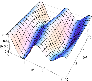
Figure 1: Plotted is $\mathcal{V}$ for $\tilde{\nu}=0.1$, $u=1$, $\gamma_{sa}=0.5$ as a function of $\theta$ and $\phi_{a}$. At $\theta=3\pi/4$ a saddle point occurs, which corresponds to $\pi$ phase jump between the two components. It is a known and dynamically unstable stationary state of the GP equations Lesanovsky and von Klitzing (2007); Brand et al. (2010).

We can see from Fig. 1 that within each large canyon in $\theta$-space, there is a secondary feature where a hill and valley form in the $\phi-$direction. We wish to focus on this relative phase feature. It is able to form a quantum field with a relativistic dispersion relation, albeit with an effective “light” velocity of very much smaller size than $c$.

III.3 Domain walls

Domain walls of relative phase appear as a connection between two degenerate vacua along a $\theta$ valley. The corresponding solution were discussed in the context of three-dimensional two-component BECs with internal coupling in Ref. Son and Stephanov (2002). In the context of one dimensional coupled BECs they are also known as atomic Josephson vortices or rotational fluxons, since they are related to circular atomic currents, and were discussed in Refs. Kaurov and Kuklov (2005, 2006); Brand et al. (2009); Qadir et al. (2012). As features of the relative phase, they only exist at sufficiently small linear coupling $\tilde{\nu}<1/3$ Kaurov and Kuklov (2005). They are unstable and can decay if a mechanism for dissipation of energy is provided unless $\tilde{\nu}\lesssim 0.14$, where they become local energy minima with topological stability Su et al. (2013). In this regime, they acquire the typical properties of topological solitons, or kinks, in the sine-Gordon equation. By tuning the coupling parameter $\tilde{\nu}$, one can thus move between regimes of different stability properties of domain walls. The regime dominated by sine-Gordon physics is found for small $\tilde{\nu}$.

IV Sine-Gordon regime

Aiming at the dynamics of the relative phase $\phi_{a}$, we simplify the action and corresponding equations of motion by assuming that all dynamics takes place in a $\theta$ valley and that both $\theta$ and $u$ only have small deviations from their respective equilibrium values. We consequently write $\theta=\pi/4+y$ and expand the action to leading orders in $y$. Using $\cos(2\theta)=-2y$, $\sin(2\theta)=1-2y^{2}$, $\cos(4\theta)=8y^{2}-1$ we obtain

$$\tilde{\mathcal{V}}={} \tilde{\nu}u^{2}\cos\phi_{a}(1-2y^{2})-\frac{\gamma_{s}}{2}u^{4}-2{\gamma_{sa}}u^{4}y^{2}$$

$$2\tilde{\mathcal{K}}={} ({\nabla}u)^{2}+u^{2}({\nabla}y)^{2}+\left\{({\nabla}\phi_{s})^{2}+({\nabla}\phi_{a})^{2}\right\}\frac{u^{2}}{4}$$

$$-{\nabla}\phi_{s}{\nabla}\phi_{a}\frac{u^{2}}{2}y$$

$$\tilde{\mathcal{L}}_{B}={} \frac{u^{2}}{2}\partial_{\tau}\phi_{s}-{u^{2}}y\partial_{\tau}\phi_{a}.$$ (20a)

Low energy dynamics is possible in two sectors: compressional waves involving $u$ and $\phi_{s}$ on the one hand, and dynamics of the relative phase involving $\phi_{a}$ and $y$ on the other. Keeping only the terms that are relevant for the latter, the Lagrangian density reads

$$\tilde{\mathcal{L}}=-u^{2}(\partial_{\tau}\phi_{a})y-\frac{u^{2}}{8}({\nabla}\phi_{a})^{2}+\tilde{\nu}u^{2}\cos(\phi_{a})-2\gamma_{sa}u^{4}y^{2}.$$ (21)

Variation with respect to the fields gives the Euler-Lagrange equation

$$\frac{\partial\mathcal{L}}{\partial f}-{\nabla}\frac{\partial\mathcal{L}}{\partial{\nabla}f}-\partial_{\tau}\frac{\partial\mathcal{L}}{\partial f_{\tau}}=0,$$ (22)

which implies that$\partial_{\tau}\phi_{a}+4\gamma_{sa}u^{2}y=0$. This allows us to replace $y$ in the Lagrangian to yield

$$\tilde{\mathcal{L}}=\frac{1}{8\gamma_{sa}}(\partial_{\tau}\phi_{a})^{2}-\frac{\tilde{n}}{4}({\nabla}\phi_{a})^{2}+2\tilde{\nu}\tilde{n}\cos(\phi_{a}).$$ (23)

This is the $D$-dimensional sine-Gordon Lagrangian.

Now we need to extract parameters. The critical speed $\tilde{c}$ is found by dividing the ${\nabla}$ pre-factor by the $\partial_{\tau}$ pre-factor and taking the square root to yield $\tilde{c}=\sqrt{2\gamma_{sa}\tilde{n}}$. The critical velocity thus matches the Bogoliubov speed of sound $\tilde{v}_{\mathrm{bog}}=\sqrt{2\gamma_{s}\tilde{n}}$ only in the case of vanishing cross coupling $\gamma_{c}$, where $\gamma_{sa}=\gamma_{s}$. We note that so far we have used classical arguments. However, our original equations are also valid as quantum field equations. If we quantize the Lagrangian, we accordingly have a quantum sine-Gordon equation, which describes the physics at sufficiently low real temperatures.

On quantizing the Lagrangian, Eq. (23), the canonical momentum field is:

$$\pi=\frac{\partial_{\tau}\phi_{a}}{4\gamma_{sa}}\,,$$

with corresponding canonical commutators of:

$$\left[\phi_{a}\left(\bm{\mathbf{\zeta}}\right),\pi\left(\bm{\mathbf{\zeta}}^{\prime}\right)\right]=i\delta^{D}\left(\bm{\mathbf{\zeta}}-\bm{\mathbf{\zeta}}^{\prime}\right)\,.$$

The sine-Gordon action can be brought into Lorenz-invariant form by rescaling time as $\zeta_{0}=\tilde{c}\tau$ to read

$$S=\hbar\int d^{D+1}\zeta\,\frac{1}{2}\left\{(\partial_{\zeta_{0}}\phi^{\prime})^{2}-({\nabla}\phi^{\prime})^{2}\right\}+\frac{\tilde{\alpha}}{\beta^{2}}\cos(\beta\phi^{\prime}),$$ (24)

with the rescaled field $\phi_{a}=\beta\phi^{\prime}$ and $\beta^{2}=2\sqrt{2\gamma_{sa}\gamma},\,\,\tilde{\alpha}=4\tilde{\nu}$. Here, $\beta^{2}$ is the universal dimensionless parameter of the quantum sine-Gordon equation. In one dimension and the case of vanishing cross coupling $\gamma_{c}=0$ and $2\gamma_{sa}=\gamma$, we obtain $\beta^{2}=2\gamma=2\sqrt{\gamma_{LL}}$, which again links to the Lieb-Liniger coupling parameter $\gamma_{LL}=mg/(\hbar^{2}n)$.

The stationary action principle leads to the (classical) sine-Gordon equation

$${{\nabla}^{2}\phi_{a}-\partial_{\zeta_{0}\zeta_{0}}\phi_{a}+\tilde{\alpha}\sin\phi_{a}=0.}$$ (25)

Note that the original field $\phi_{a}$ reappears and the parameter $\beta$ completely drops out of the classical equation. This is a relativistic field equation with a dimensionless speed of light of unity, as in all sensible relativistic field theories. Alternatively, using atomic units, we consider $\tilde{c}$ as the effective light-speed.

The parameter $\alpha=\tilde{\alpha}x_{0}^{-2}$ is connected to the characteristic length scale of the sine-Gordon equation. In physical units

$$\ell_{SG}=\frac{1}{\sqrt{{\alpha}}}=\frac{\hbar}{2\sqrt{{\nu}m}}.$$ (26)

Remarkably, this length scale depends on the tunnel coupling but is independent of the nonlinearity. It is the second characteristic length scale besides the GP healing length $x_{0}$ of Eq. (6). It sets the spatial scales of the domain walls in the sine-Gordon regime.

The parameter $\tilde{\alpha}$ is also connected to the rest mass of the elementary excitations of the sine-Gordon equation. Indeed, small amplitude oscillations $\sim\exp{-i(\tilde{\mathbf{k}}\bm{\zeta}-\tilde{\omega}_{sG}\tau)}$ of the vacuum have a relativistic dispersion relation of $\tilde{\omega}_{sG}^{2}=\tilde{k}^{2}\tilde{c}^{2}+\tilde{\alpha}\tilde{c}^{2}$, with a rest mass of $\tilde{m}_{sG}=\sqrt{\tilde{\alpha}}/\tilde{c}$ and a rest energy of $\tilde{m}_{sG}^{2}\tilde{c}^{4}=8\tilde{\nu}\gamma_{sa}\tilde{n}$. Note that the sine-Gordon light speed $\tilde{c}$ and rest mass $\tilde{m}_{sG}$ agree to leading order in $\tilde{\nu}$ with the corresponding parameters of the gapped second branch of the Bogoliubov spectrum of the stable vacuum (15). The relativistic sine-Gordon equation thus describes asymptotically a sector of excitations of the vacuum that, for small amplitude, completely decouple from the compressional waves of the Bogoliubov sound.

In the course of inflation tiny quantum fluctuations are important: they form the primordial seeds for all structure created in the later Universe. We now turn to computational quantum simulations of these equations.

V Computational Simulations

To investigate the feasibility and likely behavior of these experiments, we have carried out a number of numerical simulations of the expected dynamics. We simulated the full coupled Bose fields, using atomic densities, confinement parameters and S-wave scattering lengths generally similar to those employed in recent experimental studies with ultra-cold atoms. We employed an accurate fourth-order interaction-picture algorithm. Careful monitoring of step-size errors was needed to ensure accurate results.

The theoretical method used is a truncated, probabilistic version of the Wigner-Moyal Wigner (1932); Moyal (1947) phase-space representation Drummond and Hardman (1993); Steel et al. (1998); Sinatra et al. (2002); Blakie et al. (2008); Opanchuk and Drummond (2013). This is a probabilistic phase-space method for quantum fields, that correctly simulates symmetrically-ordered quantum dynamics in the limit of large numbers of atoms per mode. It has been shown to give results in agreement with quantum-limited photonic and BEC experiments Corney et al. (2008); Opanchuk et al. (2012), provided the large atom-number restriction is satisfied in the experiment.

Other methods of this type are also possible. One example is the positive-P representation Drummond and Gardiner (1980); Carter et al. (1987). In this normal-ordered approach, there is no truncation. Unlike the truncated Wigner method, no systematic errors occur at small occupation numbers Deuar and Drummond (2007). However, with current algorithms, the statistical sampling error grows in time for long time-scale nonlinear problems without damping. This rules out the positive-P approach for the present simulations, until better algorithms are found.

Although the resulting equations are similar to the Gross-Pitaevskii (GP) equations, the initial noise terms have a precise meaning from quantum mechanics. They correspond to the exact vacuum noise needed to generate symmetrically ordered operator moments that include the quantum fluctuations of the initial quantum state. The truncated Wigner method therefore includes quantum terms correct to order $1/n$, which are omitted in the GP approach. Additional stochastic terms are needed if there is decoherence or atomic absorption Opanchuk and Drummond (2013). However, in these preliminary studies, such effects will be omitted. We also omit the cross-coupling between spins for simplicity. Following the dimensional notation introduced previously, except that our c-number fields are now stochastic representations of quantum fields, we obtain:

$$i\partial_{\tau}\tilde{\psi}_{1} =\left\{-\frac{1}{2}{\nabla_{\zeta}}^{2}+\gamma\left|\tilde{\psi}_{1}\right|^{2}\right\}\tilde{\psi}_{1}-\tilde{\nu}\tilde{\psi}_{2},$$

$$i\partial_{\tau}\tilde{\psi}_{2} =\left\{-\frac{1}{2}{\nabla_{\zeta}}^{2}+\gamma\left|\tilde{\psi}_{2}\right|^{2}\right\}\tilde{\psi}_{2}-\tilde{\nu}\tilde{\psi}_{1}.$$ (27)

For the truncated Wigner calculations, with an initial coherent state of $\bar{\psi}(\zeta)$, so that $\tilde{\psi}(\zeta)=\bar{\psi}(\zeta)+\Delta\tilde{\psi}(\zeta)$, one would have:

$$\left\langle\Delta\tilde{\psi}(\zeta)\Delta\tilde{\psi}^{*}(\zeta^{\prime})\right\rangle=\frac{1}{2}\delta\left(\zeta-\zeta^{\prime}\right)\,.$$

We emphasize here that our assumption of an initial coherent state is certainly not the only one possible. It can be replaced by other quantum states. For example, a finite temperature ground-state followed by a sudden jump in phase is probably closer to the way that experiments will take place. Nevertheless, in the absence of a good model for the quantum state of the early universe, a coherent state is as reasonable a choice as any other.

Experimental state preparation is a complex issue, and depends on such details as the magnitude of the microwave coupling during cooling. Our initial state corresponds approximately to one in which the fields are cooled to a very weakly interacting ground state, with a coherent coupling of $\nu<0$, so that the lowest energy state has fields with an opposite sign. Then the interactions are increased to a large value, and the coupling phase is reversed to $\nu>0$, in order to create an unstable vacuum. Naturally, other models are possible, including a strongly interacting initial state at finite temperature. These will be treated elsewhere.

V.1 Dependence on couplings

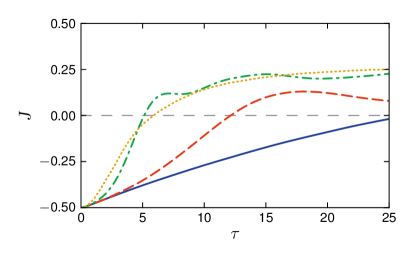
Figure 2: Decay of 1D quantum field coherence $J$, as an indicator of Sine-Gordon unstable dynamics. $\gamma=0.1$. Couplings, $\tilde{\nu}=0.001,\,0.01,\,0.1,\,1$ (blue solid, red dashed, green dash-dotted, yellow dotted). Condensate size $L=80$, 256 spatial grid points, 10000 time steps, 100 ensembles, opposite initial phases to give an unstable vacuum.

We firstly investigate the dependence of the system on the coupling strength. This is a crucial part of the calculation, as it creates the potential minimum such that the relative phase is able to be treated as an independent scalar field. The measurable quantities in an experiment are the densities obtained after interfering the two hyperfine field amplitudes Egorov et al. (2011). These are the quantities:

$$n_{\pm}=\frac{1}{2}\left\langle\left(\hat{\psi}_{1}\pm\hat{\psi}_{2}\right)^{\dagger}\left(\hat{\psi}_{1}\pm\hat{\psi}_{2}\right)\right\rangle$$ (28)

They correspond simply to the atomic densities after a rapid Rabi rotation of $\pi/2$ is performed to allow the atomic fields to interfere. Substituting the mean fields of Eq. (16) into Eq. (28), these measurable quantities are

$$n_{\pm}=u^{2}\left[\frac{1}{2}\pm\frac{1}{2}\cos\phi_{a}+O\left(y^{2}\right)\right].$$

At the vacuum phase, $\phi_{a}=0$, the atoms are all in the even mode, with $n_{+}=u^{2}$ and $n_{-}=0$. At the unstable equilibrium, $\phi_{a}=\pi$, $n_{+}=0$, and $n_{-}=u^{2}$. We plot the relative visibility, which is a quadrature-like measure of the phase, namely He et al. (2012):

$$J=\frac{\int d^{D}\bm{\zeta}\left(n_{+}-n_{-}\right)}{4N}\approx\frac{1}{2}\overline{\cos\phi_{a}}\,.$$

We see in Fig. 2, that for very weak couplings, there is a relative phase decay induced purely by quantum phase diffusion. This is the opposite to sine-Gordon physics, and occurs because the two condensates are uncoupled, and experience an increasingly random relative phase. For stronger couplings, with $\tilde{\nu}\approx 0.1$, one can see the distinctive rapid decay of an unstable vacuum, which is the signature of sine-Gordon physics with this initial condition. The slight oscillation near $\tilde{\nu}\approx 0.1$ may indicate some form of collective instability of coupled domains, and deserves further investigation.

V.2 Effects of condensate size

Although experimentally one would use a finite trap, we simulate a system with periodic boundary conditions for simplicity. To some extent, this allows us to ignore the detrimental effects of boundaries, and hence to allow a small computer simulation mimic a larger experimental condensate. However, this is not entirely the case.

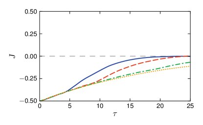
Figure 3: Decay of average 1D quantum field coherence $J$ for different condensate sizes, to indicate the effects of boundaries. Condensate size $L=10,\,20,\,40,\,80$ (blue solid, red dashed, green dash-dotted, yellow dotted), spatial grid sizes $32,\,64,\,128,\,256$, 10000 time steps, 100 ensembles, $\gamma=0.1$. Coupling $\tilde{\nu}=0$. Opposite initial phases.

As shown in Fig. 3, the finite coherence length of the quantum fluctuations has an effect on the decay statistics. Initially, the condensate size has no effect, as the coherence length is very small, and certainly much smaller than the condensate size as long as it is larger than a healing length. For increasing times, if $\tilde{\nu}=0$, the coherence length increases until it reaches the size of the condensate itself. At this stage, the decay accelerates. For very large condensates, a boundary-independent behavior is found. We note that this effect is strongest in the limit of zero coupling $\tilde{\nu}$, which is plotted here. At larger couplings the formation of domain walls limits the growth of coherence.

V.3 Single trajectory examples

Quantum mechanics only predicts ensemble averages. However, it is now common to use quantum theory to predict the behavior of the universe, which is only a single ensemble member. Of course, this experiment is not easy to repeat, especially as the observer is part of it. In the laboratory, one can obtain ensemble averages by repeating the state preparation. Even so, the density patterns and evolution in a single ensemble member is instructive. We expect the Wigner ensemble members to have a characteristic behavior like individual laboratory runs, and perhaps to the universe itself, if current theories are correct.

In the one-dimensional case, this is shown in Fig. 4. This corresponds to the largest of the condensates plotted in Fig. 3, and it is visually clear that the density correlation length is still substantially smaller than the condensate size throughout the time evolution. The local fringe visibility is defined in general as:

$$j=\frac{n_{+}-n_{-}}{2\left(n_{+}+n_{-}\right)}\approx\frac{1}{2}\cos\phi_{a}\,.$$

Since the total density is nearly constant throughout, we used the excellent approximation of $j\approx\left(n_{+}-n_{-}\right)/(2\bar{u}^{2})$ for simplicity of calculation and plotting.

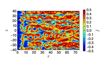
Figure 4: Plot of 1D space-time dynamics of the local visibility $j$ for a single trajectory, showing contour plot vs time and space. Coupling $\tilde{\nu}=0.1$, condensate size 80, 256 spatial grid points, $\gamma=0.1$, 10000 time steps.

V.4 Two-dimensional behavior

The universe is certainly not one-dimensional. Anyone might reasonably question the applicability of a one-dimensional simulation, even though this is the most amenable to theoretical treatment. In the laboratory, the availability of engineered traps means that dimensionality can be readily adjusted to obtain artificial universes of one, two or three space dimensions.

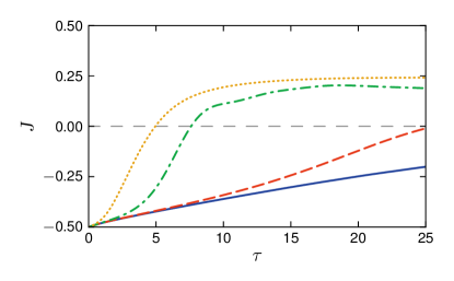
Figure 5: Plot of 2D quantum field coherence $J$, as an indicator of sine-Gordon unstable dynamics. $\gamma=0.1$. Couplings, $\tilde{\nu}=0.001,\,0.01,\,0.1,\,1$ (blue solid, red dashed, green dash-dotted, yellow dotted). Condensate size $L=80$, $256\times 256$ spatial grid points, 4000 time steps, 200 ensembles, opposite initial phases.

The average dynamics of the sine-Gordon field depend on dimensionality as shown in Fig. 5, which shows that the two-dimensional averages differ from Fig. 2, although there are qualitative similarities. However, Fig. 6 is much more interesting, demonstrating clearly the growth of complex spatial structures. These are two-dimensional cross-sections, taken at dimensionless times of $\tau=5$,$\tau=10$ and$\tau=20$. These single-trajectory plots show how the early, relatively high momentum quantum noise patterns have decayed into coherent spatial domains with a typical spatial coherence length of order $\bar{\zeta}=10$ spatial units at $\tau=10$, and start to evaporate at later times. It remains to be investigated whether this later evaporation is an artifact of the coupled BEC system, or a genuine sine-Gordon feature.

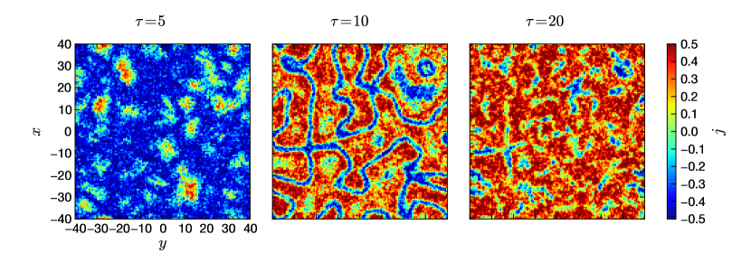
Figure 6: Plot of 2D spacial clustering of the local visibility $j$ for a single trajectory, showing contour plot vs space at final time. Coupling $\tilde{\nu}=0.1$, condensate size $80\times 80$, $128\times 128$ spatial grid points, $\gamma=0.1$, 5000 time steps, opposite initial phases, time $\tau=10$.

V.5 Three-dimensional behavior

Recent experiments have shown the possibility of exploring a condensate in a “can” or cylindrical trap. This is a flat trap in three-dimensions, with reflecting boundary conditions. While our simulations do not have this type of boundary, it is feasible to carry out large three-dimensional calculations relatively quickly using GPU hardware Opanchuk et al. (2012). In Fig. 7, we show a slice through a condensate, in which one coordinate is held fixed, while the other two are varied. This is a single ensemble member, and the other parameters are similar to the two-dimensional case, Fig. 6.

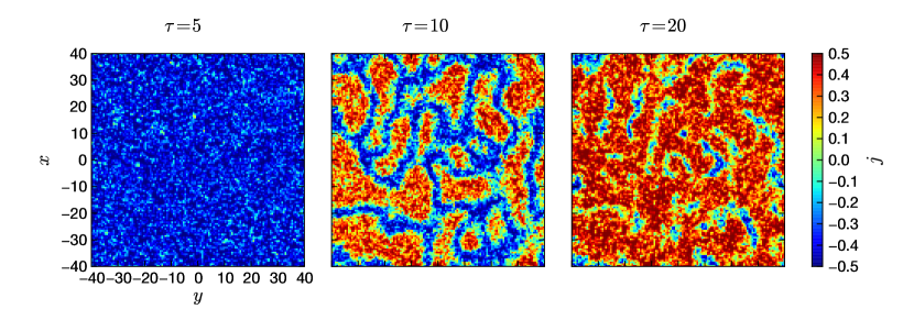
Figure 7: Plot of 3D spacial clustering geometry of the local visibility $j$ for single trajectory, showing contour plot vs space, sliced through a single z-coordinate. Coupling $\tilde{\nu}=0.1$, condensate size $80\times 80\times 80$, $128\times 128\times 128$ spatial grid points, $\gamma=0.1$, 5000 time steps, opposite initial phases. Plotted: a slice orthogonal to x-axis at $\tau=10$.

The resulting spatial geometry of clusters of hot and cold matter is distinctly different to the two-dimensional case, with greater connectedness, as larger coherent structures are formed over the same time-scale. Here we have plotted the real spatial image of a two-dimensional slice, to show domain-like clustering effects. This demonstrates that very large-scale clustering effects occur even in the absence of explicit gravitational interactions, for our model.

Rapid progress in imaging technology means that it is now possible to image such 2D slices in the experiment Bücker et al. (2009), although it is technologically more difficult than typical BEC experimental techniques which produce a column density image of an expanded condensate.

VI Summary

The general behavior and unstable dynamics of an effective quantum sine-Gordon field using a two-mode BEC with linear coupling has been clearly demonstrated. Experimentally, for the scenario outlined here, it is important to use an atomic species whose cross-coupling differs from its self-coupling. This largely rules out the most commonly used atomic species, ${}^{87}Rb$, which has very similar self and cross couplings apart from a small region near a Feshbach resonance. A Feshbach-type experiment is still possible, although losses are greater in this regime. Apart from this case, there are many species which are both able to be evaporatively cooled and have multiple hyperfine levels. For example,${}^{39}K$ can be used. It has a sizable difference of $g_{1}g_{2}-g_{c}^{2}$ D’Errico et al. (2007); Chin et al. (2010), and it is therefore more suitable for realization of our proposal.

Our results will be extended to a more complete analysis of the numerical simulations elsewhere, in which we will analyze in greater detail the effects of different types of state preparation. However, it is clear that in principle the use of ultra-cold quantum gases as quantum simulators is not restricted to condensed matter and non-relativistic analogies. Simulating interacting relativistic quantum fields in one, two or three dimensions appears completely feasible, both experimentally and computationally. An experimental implementation would throw much-needed light on the question of how accurate our numerical approximations are for these parameter values.

While we have focused on the practical issues of how to carry out the experiment and corresponding numerical simulations, these issues pale somewhat in comparison to another issue. We hope our proposal will stimulate interest in this fundamental question, which is:

• how do we carry out measurements on the quantum universe, when we are part of it?

References

- Porras and Cirac (2004) D. Porras and J. I. Cirac, Phys. Rev. Lett. 92, 207901 (2004).
- Higgs (1964a) P. W. Higgs, Phys. Lett. 12, 132 (1964a).
- Englert and Brout (1964) F. Englert and R. Brout, Phys. Rev. Lett. 13, 321 (1964).
- Higgs (1964b) P. W. Higgs, Phys. Rev. Lett. 13, 508 (1964b).
- Guralnik et al. (1964) G. Guralnik, C. Hagen, and T. Kibble, Phys. Rev. Lett. 13, 585 (1964).
- Coleman (1977) S. Coleman, Phys. Rev. D 15, 2929 (1977).
- Callan and Coleman (1977) C. Callan and S. Coleman, Phys. Rev. D 16, 1762 (1977).
- Guth (1981) A. H. Guth, Phys. Rev. D 23, 347 (1981).
- Linde (1991) A. Linde, Phys. Lett. B 259, 38 (1991).
- Linde (1994) A. Linde, Phys. Rev. D 49, 748 (1994).
- Linde (1998) A. Linde, Phys. Rev. D 58, 083514 (1998).
- Stewart and Lyth (1993) E. D. Stewart and D. H. Lyth, Phys. Lett. B 302, 171 (1993).
- Liddle et al. (1994) A. Liddle, P. Parsons, and J. Barrow, Phys. Rev. D 50, 7222 (1994).
- Fischer and Schützhold (2004) U. Fischer and R. Schützhold, Phys. Rev. A 70, 063615 (2004).
- Neuenhahn et al. (2012) C. Neuenhahn, A. Polkovnikov, and F. Marquardt, Phys. Rev. Lett. 109, 085304 (2012).
- ATLAS Collaboration (2012) ATLAS Collaboration, Phys. Lett. B 716, 1 (2012).
- CMS Collaboration (2012) CMS Collaboration, Phys. Lett. B 716, 30 (2012).
- Egorov et al. (2011) M. Egorov, R. P. Anderson, V. Ivannikov, B. Opanchuk, P. D. Drummond, B. V. Hall, and A. I. Sidorov, Phys. Rev. A 84, 021605(R) (2011).
- Gring et al. (2012) M. Gring, M. Kuhnert, T. Langen, T. Kitagawa, B. Rauer, M. Schreitl, I. Mazets, D. A. Smith, E. Demler, and J. Schmiedmayer, Science 337, 1318 (2012).
- Gaunt et al. (2013) A. L. Gaunt, T. F. Schmidutz, I. Gotlibovych, R. P. Smith, and Z. Hadzibabic, Phys. Rev. Lett. 110, 200406 (2013).
- Planck Collaboration (2013) Planck Collaboration, “Planck 2013 results. I. Overview of products and scientific results,” arXiv:1303.5062 (2013).
- Kaurov and Kuklov (2006) V. Kaurov and A. Kuklov, Phys. Rev. A 73, 013627 (2006).
- Gritsev et al. (2007) V. Gritsev, A. Polkovnikov, and E. Demler, Phys. Rev. B 75, 174511 (2007).
- Son and Stephanov (2002) D. Son and M. Stephanov, Phys. Rev. A 65, 063621 (2002).
- Lieb and Liniger (1963) E. H. Lieb and W. Liniger, Phys. Rev. 130, 1605 (1963).
- Brand et al. (2010) J. Brand, T. J. Haigh, and U. Zülicke, Phys. Rev. A 81, 025602 (2010).
- Lesanovsky and von Klitzing (2007) I. Lesanovsky and W. von Klitzing, Phys. Rev. Lett. 98, 050401 (2007).
- Montgomery et al. (2010) T. W. A. Montgomery, R. G. Scott, I. Lesanovsky, and T. M. Fromhold, Phys. Rev. A 81, 063611 (2010).
- Esry et al. (1997) B. D. Esry, C. Greene, J. Burke, Jr., and J. Bohn, Phys. Rev. Lett. 78, 3594 (1997).
- Kaurov and Kuklov (2005) V. Kaurov and A. Kuklov, Phys. Rev. A 71, 011601 (2005).
- Brand et al. (2009) J. Brand, T. J. Haigh, and U. Zülicke, Phys. Rev. A 80, 011602 (2009).
- Qadir et al. (2012) M. I. Qadir, H. Susanto, and P. C. Matthews, J. Phys. B 45, 035004 (2012).
- Su et al. (2013) S.-W. Su, S.-C. Gou, A. S. Bradley, O. Fialko, and J. Brand, “Kibble-Zurek scaling and its breakdown for spontaneous generation of Josephson vortices in Bose-Einstein condensates,” arXiv:1302.3304 (2013).
- Wigner (1932) E. P. Wigner, Phys. Rev. 40, 749 (1932).
- Moyal (1947) J. E. Moyal, Math. Proc. Cambridge 45, 99 (1947).
- Drummond and Hardman (1993) P. D. Drummond and A. D. Hardman, Europhys. Lett. 21, 279 (1993).
- Steel et al. (1998) M. Steel, M. K. Olsen, L. I. Plimak, P. D. Drummond, S. Tan, M. J. Collett, D. F. Walls, and R. Graham, Phys. Rev. A 58, 4824 (1998).
- Sinatra et al. (2002) A. Sinatra, C. Lobo, and Y. Castin, J. Phys. B 35, 3599 (2002).
- Blakie et al. (2008) P. B. Blakie, A. S. Bradley, M. J. Davis, R. J. Ballagh, and C. W. Gardiner, Adv. Phys. 57, 363 (2008).
- Opanchuk and Drummond (2013) B. Opanchuk and P. D. Drummond, J. Math. Phys. 54, 042107 (2013).
- Corney et al. (2008) J. F. Corney, J. Heersink, R. Dong, V. Josse, P. D. Drummond, G. Leuchs, and U. L. Andersen, Phys. Rev. A 78, 023831 (2008).
- Opanchuk et al. (2012) B. Opanchuk, M. Egorov, S. E. Hoffmann, A. I. Sidorov, and P. D. Drummond, Europhys. Lett. 97, 50003 (2012).
- Drummond and Gardiner (1980) P. D. Drummond and C. W. Gardiner, J. Phys. A: Math. Gen. 13, 2353 (1980).
- Carter et al. (1987) S. J. Carter, P. D. Drummond, M. D. Reid, and R. M. Shelby, Phys. Rev. Lett. 58, 1841 (1987).
- Deuar and Drummond (2007) P. P. Deuar and P. D. Drummond, Phys. Rev. Lett. 98, 120402 (2007).
- He et al. (2012) Q.-Y. He, T. G. Vaughan, P. D. Drummond, and M. D. Reid, New J. Phys. 14, 093012 (2012).
- Bücker et al. (2009) R. Bücker, A. Perrin, S. Manz, T. Betz, C. Koller, T. Plisson, J. Rottmann, T. Schumm, and J. Schmiedmayer, New J. Phys. 11, 103039 (2009).
- D’Errico et al. (2007) C. D’Errico, M. Zaccanti, M. Fattori, G. Roati, M. Inguscio, G. Modugno, and A. Simoni, New J. Phys. 9, 223 (2007).
- Chin et al. (2010) C. Chin, R. Grimm, P. Julienne, and E. Tiesinga, Rev. Mod. Phys. 82, 1225 (2010).