A Supervised Neural Autoregressive Topic Model for Simultaneous Image Classification and Annotation

Abstract

Topic modeling based on latent Dirichlet allocation (LDA) has been a framework of choice to perform scene recognition and annotation. Recently, a new type of topic model called the Document Neural Autoregressive Distribution Estimator (DocNADE) was proposed and demonstrated state-of-the-art performance for document modeling. In this work, we show how to successfully apply and extend this model to the context of visual scene modeling. Specifically, we propose SupDocNADE, a supervised extension of DocNADE, that increases the discriminative power of the hidden topic features by incorporating label information into the training objective of the model. We also describe how to leverage information about the spatial position of the visual words and how to embed additional image annotations, so as to simultaneously perform image classification and annotation. We test our model on the Scene15, LabelMe and UIUC-Sports datasets and show that it compares favorably to other topic models such as the supervised variant of LDA.

1 Introduction

Image classification and annotation are two important tasks in computer vision. In image classification, one tries to describe the image globally with a single descriptive label (such as coast, outdoor, inside city, etc.), while annotation focuses on tagging the local content within the image (such as whether it contains “sky”, a “car”, a “tree”, etc.). Since these two problems are related, it is natural to attempt to solve them jointly. For example, an image labeled as street is more likely to be annotated with “car”, “pedestrian” or “building” than with “beach” or “see water”. Although there has been a lot of work on image classification and annotation separately, less work has looked at solving these two problems simultaneously.

Work on image classification and annotation is often based on a topic model, the most popular being latent Dirichlet allocation or LDA [1]. LDA is a generative model for documents that originates from the natural language processing community but that has had great success in computer vision for scene modeling [1, 2]. LDA models a document as a multinomial distribution over topics, where a topic is itself a multinomial distribution over words. While the distribution over topics is specific for each document, the topic-dependent distributions over words are shared across all documents. Topic models can thus extract a meaningful, semantic representation from a document by inferring its latent distribution over topics from the words it contains. In the context of computer vision, LDA can be used by first extracting so-called “visual words” from images, convert the images into visual word documents and training an LDA topic model on the bags of visual words. Image representations learned with LDA have been used successfully for many computer vision tasks such as visual classification [3, 4], annotation [5, 6] and image retrieval [7, 8].

Although the original LDA topic model was proposed as an unsupervised learning method, supervised variants of LDA have been proposed [9, 2]. By modeling both the documents’ visual words and their class labels, the discriminative power of the learned image representations could thus be improved.

At the heart of most topic models is a generative story in which the image’s latent representation is generated first and the visual words are subsequently produced from this representation. The appeal of this approach is that the task of extracting the representation from observations is easily framed as a probabilistic inference problem, for which many general purpose solutions exist. The disadvantage however is that as a model becomes more sophisticated, inference becomes less trivial and more computationally expensive. In LDA for instance, inference of the distribution over topics does not have a closed-form solution and must be approximated, either using variational approximate inference or MCMC sampling. Yet, the model is actually relatively simple, making certain simplifying independence assumptions such the conditional independence of the visual words given the image’s latent distribution over topics.

Recently, an alternative generative modeling approach for documents was proposed by Larochelle and Lauly [10]. Their model, the Document Neural Autoregressive Distribution Estimator (DocNADE), models directly the joint distribution of the words in a document, by decomposing it through the probability chain rule as a product of conditional distributions and modeling each conditional using a neural network. Hence, DocNADE doesn’t incorporate any latent random variables over which potentially expensive inference must be performed. Instead, a document representation can be computed efficiently in a simple feed-forward fashion, using the value of the neural network’s hidden layer. Larochelle and Lauly [10] also show that DocNADE is a better generative model of text documents and can extract a useful representation for text information retrieval.

In this paper, we consider the application of DocNADE in the context of computer vision. More specifically, we propose a supervised variant of DocNADE (SupDocNADE), which models the joint distribution over an image’s visual words, annotation words and class label. The model is illustrated in Figure 1. We investigate how to successfully incorporate spatial information about the visual words and highlight the importance of calibrating the generative and discriminative components of the training objective. Our results confirm that this approach can outperform the supervised variant of LDA and is a competitive alternative for scene modeling.

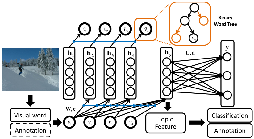
Figure 1: Illustration of SupDocNADE for joint classification and annotation of images. Visual and annotation words are extracted from images and modeled by SupDocNADE, which models the joint distribution of the words ${\bf v}=[v_{1},\dots,v_{D}]$ and class label $y$ as $p({\bf v},y)=p(y|{\bf v})\prod_{i}p(v_{i}|v_{1},\dots,v_{i-1})$. All conditionals $p(y|{\bf v})$ and $p(v_{i}|v_{1},\dots,v_{i-1})$ are modeled using neural networks with shared weights. Each predictive word conditional $p(v_{i}|v_{1},\dots,v_{i-1})$ (noted ${\hat{v}}_{i}$ for brevity) follows a tree decomposition where each leaf is a possible word. At test time, the annotation words are not used (illustrated with a dotted box) to compute the image’s topic feature representation.

2 Related Work

Simultaneous image classification and annotation is often addressed using models extending the basic LDA topic model. Wang et al. [2] proposed a supervised LDA formulation to tackle this problem. Wang and Mori [11] opted instead for a maximum margin formulation of LDA (MMLDA). Our work also belongs to this line of work, extending topic models to a supervised computer vision problem: our contribution is to extend a different topic model, DocNADE, to this context.

What distinguishes DocNADE from other topic models is its reliance on a neural network architecture. Neural networks are increasingly used for the probabilistic modeling of images (see [12] for a review). In the realm of document modeling, Salakhutdinov and Hinton [13] proposed a Replicated Softmax model for bags of words. DocNADE is in fact inspired by that model and was shown to improve over its performance while being much more computationally efficient. Wan et al. [14] also proposed a hybrid model that combines LDA and a neural network. They applied their model to scene classification only, outperforming approaches based on LDA or on a neural network only. In our experiments, we show that our approach outperforms theirs. Generally speaking, we are not aware of any other work which has considered the problem of jointly classifying and annotating images using a hybrid topic model/neural network approach.

3 Document NADE

In this section, we describe the original DocNADE model. In Larochelle and Lauly [10], DocNADE was use to model documents of real words, belonging to some predefined vocabulary. To model image data, we assume that images have first been converted into a bag of visual words. A standard approach is to learn a vocabulary of visual words by performing $K$-means clustering on SIFT descriptors densely exacted from all training images. See Section 5.2 for more details about this procedure. From that point on, any image can thus be represented as a bag of visual words ${\bf v}=[v_{1},v_{2},\ldots,v_{D}]$, where each $v_{i}$ is the index of the closest $K$-means cluster to the $i^{\rm th}$ SIFT descriptor extracted from the image and $D$ is the number of extracted descriptors.

DocNADE models the joint probability of the visual words $p({\bf v})$ by rewritting it as

$$p\left({\bf v}\right)=\prod_{i=1}^{D}p\left(v_{i}|{\bf v}_{<i}\right)$$ (1)

and modeling instead each conditional $p(v_{i}|{\bf v}_{<i})$, where $\mathbf{v}_{<i}$ is the subvector containing all $v_{j}$ such that $j<i$. Notice that Equation 1 is true for any distribution, based on the probability chain rule. Hence, the main assumption made by DocNADE is in the form of the conditionals. Specifically, DocNADE assumes that each conditional can be modeled and learned by a feedforward neural network.

One possibility would be to model $p(v_{i}|\mathbf{v}_{<i})$ with the following architecture:

$$\mathbf{h}_{i}\left(\mathbf{v}_{<i}\right)={\bf g}\left(\mathbf{c}+\sum_{k<i}\mathbf{W}_{:,v_{k}}\right), p\left(v_{i}=w|\mathbf{v}_{<i}\right)=\frac{\exp\left(b_{w}+\mathbf{V}_{w,:}\mathbf{h}_{i}\left(\mathbf{v}_{<i}\right)\right)}{\sum_{w{}^{\prime}}\exp\left(b_{w{}^{\prime}}+\mathbf{V}_{w{}^{\prime},:}\mathbf{h}_{i}\left(\mathbf{v}_{<i}\right)\right)}$$ (2)

where $g(\cdot)$ is an element-wise non-linear activation function, $\mathbf{W}\in\mathbb{R}^{H\times K}$ and $\mathbf{V}\in\mathbb{R}^{K\times H}$ are the connection parameter matrices, $\mathbf{c}\in\mathbb{R}^{N}$ and $\mathbf{b}\in\mathbb{R}^{K}$ are bias parameter vectors and $H,K$ are the number of hidden units (topics) and vocabulary size, respectively.

Computing the distribution $p(v_{i}=w|\mathbf{v}_{<i})$ of Equation 2 requires time linear in $K$. In practice, this is too expensive, since it must be computed for each of the $D$ visual words $v_{i}$. To address this issue, Larochelle and Lauly [10] propose to use a balanced binary tree to decompose the computation of the conditionals and obtain a complexity logarithmic in $K$. This is achieved by randomly assigning all visual words to a different leaf in a binary tree. Given this tree, the probability of a word is modeled as the probability of reaching its associated leaf from the root. We model each left/right transition probabilities in the binary tree using a set of binary logistic regressors taking the hidden layer $\mathbf{h}_{i}({\bf v}_{<i})$ as input. The probability of a given word can then be obtained by multiplying the probabilities of each left/right choices of the associated tree path.

Specifically, let $\mathbf{l}\left(v_{i}\right)$ be the sequence of tree nodes on the path from the root to the leaf of $v_{i}$ and let $\pi\left(v_{i}\right)$ be the sequence of binary left/right choices at the internal nodes along that path. For example, $l\left(v_{i}\right)_{1}$ will always be the root node of the binary tree, and $\pi\left(v_{i}\right)_{1}$ will be $0$ if the word leaf $v_{i}$ is in the left subtree or $1$ otherwise. Let $\mathbf{V}\in\mathbb{R}^{T\times H}$ now be the matrix containing the logistic regression weights and $\mathbf{b}\in\mathbb{R}^{T}$ be a vector containing the biases, where $T$ is the number of inner nodes in the binary tree and $H$ is the number of hidden units. The probability $p(v_{i}=w|\mathbf{v}_{<i})$ is now modeled as

$$p(v_{i}=w|\mathbf{v}_{<i})=\prod_{k=1}^{|\pi\left(v_{i}\right)|}p(\pi\left(v_{i}\right)_{k}|\mathbf{v}_{<i})~{},$$ (3)

where

$$p(\pi\left(v_{i}\right)_{k}=1|\mathbf{v}_{<i})=\textup{ sigm}\left(b_{l\left(v_{i}\right)_{m}}+\mathbf{V}_{l\left(v_{i}\right)_{m},:}\mathbf{h}_{i}\left(\mathbf{v}_{<i}\right)\right)$$ (4)

are the internal node logistic regression outputs and $\textup{ sigm}(x)=1/(1+\exp(-x))$ is the sigmoid function. By using a balanced tree, we are guaranteed that computing Equation 3 involves only $O(\log K)$ logistic regression outputs. One could attempt to optimize the organization of the words within the tree, but a random assignment of the words to leaves works well in practice [10].

Thus, by combining Equations 2, 3 and 4, we can compute the probability $p\left({\bf v}\right)=\prod_{i=1}p\left(v_{i}|{\bf v}_{<i}\right)$ for any document under DocNADE. To train the parameters $\theta=\{{{\bf W},{\bf V},{\bf b},{\bf c}\}}$ of DocNADE, we simply optimize the average negative log-likelihood of the training set documents using stochastic gradient descent. Once the model is trained, a latent representation can be extracted from a new document $\mathbf{v^{\ast}}$ as follows:

$$\mathbf{h}_{y}\left(\mathbf{v}^{\ast}\right)={\bf g}\left(\mathbf{c}+\sum_{i}^{D}\mathbf{W}_{:,v^{\ast}_{i}}\right)~{}.$$ (5)

This representation could be fed to a standard classifier to perform any supervised computer vision task. The index $y$ is used to highlight that it is the representation used to predict the class label $y$ of the image.

Equations 3,4 indicate that the conditional probability of each word $v_{i}$ requires computing the position dependent hidden layer $\mathbf{h}_{i}\left(\mathbf{v}_{<i}\right)$, which extracts a representation out of the bag of previous visual words $\mathbf{v}_{<i}$. Since computing $\mathbf{h}_{i}\left(\mathbf{v}_{<i}\right)$ is in $O(HD)$ on average, and there are $D$ hidden layers $\mathbf{h}_{i}\left(\mathbf{v}_{<i}\right)$ to compute, then a naive procedure for computing all hidden layers would be in $O(HD^{2})$.

However, noticing that

$${\mathbf{h}_{i+1}\left(\mathbf{v}_{<i+1}\right)} = {\bf g}\left(\mathbf{c}+\sum_{k<i+1}\mathbf{W}_{:,v_{k}}\right)={\bf g}\left(\mathbf{W}_{:,v_{i}}+\mathbf{c}+\sum_{k<i}\mathbf{W}_{:,v_{k}}\right)$$ (6)

and exploiting that fact that the weight matrix $\mathbf{W}$ is the same across all conditionals, the linear transformation $\mathbf{c}+\sum_{k<i}\mathbf{W}_{:,v_{k}}$ can be reused from the computation of the previous hidden layer $\mathbf{h}_{i}(\mathbf{v}_{<i})$ to compute $\mathbf{h}_{i+1}(\mathbf{v}_{<i+1})$. With this procedure, computing all hidden layers $\mathbf{h}_{i}(\mathbf{v}_{<i})$ sequentially from $i=1$ to $i=D$ becomes in $O(HD)$.

Finally, since the computation complexity of each of the $O(\log K)$ logistic regressions in Equation 3 is $O(H)$, the total complexity of computing $p(v_{i}=w|\mathbf{v}_{<i})$ is $O(\log(K)HD)$. In practice, the length of document $D$ and the number of hidden units $H$ tends to be small, while $\log(K)$ will be small even for large vocabularies. Thus DocNADE can be used and trained efficiently.

4 SupDocNADE for Image Classification and Annotation

In this section, we describe the approach of this paper, inspired by DocNADE, to simultaneously classify and annotate image data. First, we describe a supervised extension of DocNADE (SupDocNADE), which incorporates class label information into training to learn more discriminative hidden features for classification. Then we describe how we exploit the spatial position information of the visual words. At last, we describe how to also perform annotation, along with classification, using SupDocNADE.

4.1 Supervised DocNADE

It has been observed that learning image feature representations using unsupervised topic models such as LDA can perform worse than training a classifier directly on the visual words themselves, using an appropriate kernel such as a pyramid kernel [3]. One reason is that the unsupervised topic features are trained to explain as much of the entire statistical structure of images as possible and might not model well the particular discriminative structure we are after in our computer vision task. This issue has been addressed in the literature by devising supervised variants of LDA, such as Supervised LDA or sLDA [9]. DocNADE also being an unsupervised topic model, we propose here a supervised variant of DocNADE, SupDocNADE, in an attempt to make the learned image representation more discriminative for the purpose of image classification.

Specifically, given an image ${\bf v}=[v_{1},v_{2},\ldots,v_{D}]$ and its class label $y\in\{1,\dots,C\}$, SupDocNADE models the full joint distribution as

$$p({\bf v})=p(y|{\bf v})\prod_{i=1}^{D}p\left(v_{i}|{\bf v}_{<i}\right)~{}~{}.$$ (7)

As in DocNADE, each conditional is modeled by a neural network. We use the same architecture for $p\left(v_{i}|{\bf v}_{<i}\right)$ as in regular DocNADE. We now only need to define the model for $p(y|{\bf v})$.

Since $\mathbf{h}_{y}\left(\mathbf{v}\right)$ is the image representation that we’ll use to perform classification, we propose to model $p\left(y|{\bf v}\right)$ as a multiclass logistic regression output computed from $\mathbf{h}_{y}\left(\mathbf{v}\right)$:

$$p\left(y|{\bf v}\right)={\rm softmax}\left(\mathbf{d}+\mathbf{U}\mathbf{h}_{y}\left(\mathbf{v}\right)\right)_{y}$$ (8)

where ${\rm softmax}({\bf a})_{i}=\exp(a_{i})/\sum_{j=1}^{C}\exp(a_{j})$, $\mathbf{d}\in\mathbb{R}^{C}$ is the bias parameter vector in the supervised layer and $\mathbf{U}\in\mathbb{R}^{C\times H}$ is the connection matrix between hidden layer $\mathbf{h}_{y}$ and the class label.

Put differently, $p\left(y|{\bf v}\right)$ is modeled as a regular multiclass neural network, taking as input the bag of visual words ${\bf v}$. The crucial difference however with a regular neural network is that some of its parameters (namely the hidden unit parameters ${\bf W}$ and ${\bf c}$) are also used to model the visual word conditionals $p\left(v_{i}|{\bf v}_{<i}\right)$.

Maximum likelihood training of this model is performed by minimizing the negative log-likelihood

$$-\log p\left({\bf v},y\right)=-\log p\left(y|{\bf v}\right)+\sum_{i=1}^{D}-\log p(v_{i}|{\bf v}_{i})$$ (9)

averaged over all training images. This is known as generative learning [15]. The first term is a purely discriminative term, while the second is unsupervised and can be understood as a regularizer, that encourages a solution which also explains the unsupervised statistical structure within the visual words. In practice, this regularizer can bias the solution too strongly away from a more discriminative solution that generalizes well. Hence, similarly to previous work on hybrid generative/discriminative learning, we propose instead to weight the importance of the generative term

$$-\log p\left({\bf v},y\right)=-\log p\left(y|{\bf v}\right)+\lambda\sum_{i=1}^{D}-\log p(v_{i}|{\bf v}_{i})$$ (10)

where $\lambda$ is treated as a regularization hyper-parameter.

Training on the training set average of Equation 10 is performed by stochastic gradient descent, using backpropagation to compute the parameter derivatives. As in regular DocNADE, computation of the training objective and its gradient requires that we define an ordering of the visual words. Though we could have defined an arbitrary path across the image to order the words (e.g. from left to right, top to bottom in the image), we follow Larochelle and Lauly [10] and randomly permute the words before every stochastic gradient update. The implication is that the model is effectively trained to be a good inference model of any conditional $p(v_{i}|{\bf v}_{<i})$, for any ordering of the words in ${\bf v}$. This again helps fighting against overfitting and better regularizes our model.

In our experiments, we used the rectified linear function as the activation function

$${\bf g}({\bf a})=\max(0,{\bf a})=[\max(0,a_{1}),\dots,\max(0,a_{H})]$$ (11)

which often outperforms other activation functions [16] and has been shown to work well for image data [17]. Since this is a piece-wise linear function, the (sub-)gradient with respect to its input, needed by backpropagation to compute the parameter gradients, is simply

$${\bf 1}_{({\bf g}({\bf a})>0)}=[1_{(g(a_{1})>0)},\dots,1_{(g(a_{H})>0)}]$$ (12)

where $1_{P}$ is 1 if $P$ is true and 0 otherwise. Algorithms 1 and 2 give pseudocodes for efficiently computing the joint distribution $p\left({\bf v},y\right)$ and the parameter gradients of Equation 10 required for stochastic gradient descent training.

Algorithm 1 Computing $p\left({\bf v},y\right)$ using SupDocNADE

  Input: bag of words representation ${\bf v}$, target $y$

  Output: $p\left({\bf v},y\right)$

  $\mathbf{a}\leftarrow\mathbf{c}$

  $p\left(\mathbf{v}\right)\leftarrow 1$

  for $i$ from $1$ to $D$ do

     $\mathbf{h}_{i}\leftarrow$ ${\bf g}\left(\mathbf{a}\right)$

     $p\left(v_{i}|\mathbf{v}_{<i}\right)=1$

     for $m$ from 1 to $|\pi\left(v_{i}\right)|$ do

        $p\left(v_{i}|\mathbf{v}_{<i}\right)\leftarrow p\left(v_{i}|\mathbf{v}_{<i}\right)p\left(\pi\left(v_{i}\right)_{m}|\mathbf{v}_{<i}\right)$

     end for

     $p\left(\mathbf{v}\right)\leftarrow p\left(\mathbf{v}\right)p\left(v_{i}|\mathbf{v}_{<i}\right)$

     $\mathbf{a}\leftarrow\mathbf{a}+\mathbf{W}_{:,v_{i}}$

  end for

  $\mathbf{h}^{c}\left(\mathbf{v}\right)\leftarrow\max(0,\mathbf{a})$

  $p\left(y|\mathbf{v}\right)\leftarrow\textup{softmax}\left(\mathbf{d}+\mathbf{U}\mathbf{h}^{c}\left(\mathbf{v}\right))\right)_{|y}$

  $p\left({\bf v},y\right)\leftarrow p\left(\mathbf{v}\right)p\left(y|\mathbf{v}\right)$

Algorithm 2 Computing SupDocNADE training gradients

  Input: training vector ${\bf v}$, target $y$,          unsupervised learning weight $\lambda$

  Output: gradients of Equation 10 w.r.t. parameters

  $f\left(\mathbf{v}\right)\leftarrow\textup{softmax}\left(\mathbf{d}+\mathbf{U}\mathbf{h}^{c}\left(\mathbf{v}\right))\right)$

  $\delta\mathbf{d}\leftarrow\left(f\left(\mathbf{v}\right)-1_{y}\right)$

  $\delta\mathbf{a}\leftarrow(\mathbf{U}^{\intercal}\delta\mathbf{d})\circ 1_{{\bf h}_{y}>0}$

  $\delta\mathbf{U}\leftarrow\delta\mathbf{d}~{}{\mathbf{h}^{c^{\intercal}}}$

  $\delta\mathbf{c}\leftarrow 0$, $\delta\mathbf{b}\leftarrow 0$, $\delta\mathbf{V}\leftarrow 0$, $\delta\mathbf{W}\leftarrow 0$

  for $i$ from $D$ to $1$ do

     $\delta\mathbf{h}_{i}\leftarrow 0$

     for $m$ from $1$ to $|\pi\left(v_{i}\right)|$ do

        $\delta t\leftarrow\lambda\left(p\left(\pi\left(v_{i}\right)_{m}|\mathbf{v}_{<i}\right)-\pi\left(v_{i}\right)_{m}\right)$

        $\delta b_{l\left(v_{i}\right)_{m}}\leftarrow\delta b_{l\left(v_{i}\right)_{m}}+\delta t$

        $\delta\mathbf{V}_{l\left(v_{i}\right)_{m},:}\leftarrow\delta\mathbf{V}_{l\left(v_{i}\right)_{m},:}+\delta t~{}\mathbf{h}_{i}^{\intercal}$

        $\delta\mathbf{h}_{i}\leftarrow\delta\mathbf{h}_{i}+\delta t~{}\mathbf{V}_{l\left(v_{i}\right)_{m},:}^{\intercal}$

     end for

     $\delta\mathbf{a}\leftarrow\delta\mathbf{a}+\delta\mathbf{h}_{i}\circ 1_{{\bf h}_{i}>0}$

     $\delta\mathbf{c}\leftarrow\delta\mathbf{c}+\delta\mathbf{h}_{i}\circ 1_{{\bf h}_{i}>0}$

     $\delta\mathbf{W}_{:,v_{i}}\leftarrow\delta\mathbf{W}_{:,v_{i}}+\delta\mathbf{a}$

  end for

4.2 Dealing with Multiple Regions

Spatial information plays an important role for understanding an image. For example, the sky will often appear on the top part of the image, while a car will most often appear at the bottom. A lot of previous work has exploited this intuition successfully. For example, in the seminal work on spatial pyramids [3], it is shown that extracting different visual word histograms over distinct regions instead of a single image-wide histogram can yield substantial gains in performance.

We follow a similar approach, whereby we model both the presence of the visual words and the identity of the region they appear in. Specifically, let’s assume the image is divided into several distinct regions ${\cal R}=\{{R_{1},R_{2},\ldots,R_{M}\}}$, where $M$ is the number of regions. The image can now be represented as

$${\bf v}^{\cal R} = [v^{\cal R}_{1},v^{\cal R}_{2},\ldots,v^{\cal R}_{D}]=[\left(v_{1},r_{1}\right),\left(v_{2},r_{2}\right),\ldots,\left(v_{D},r_{D}\right)]$$ (13)

where $r_{i}\in{\cal R}$ is the region from which the visual word $v_{i}$ was extracted. To model the joint distribution over these visual words, we decompose it as $p({\bf v}^{\cal R})=\prod_{i}p((v_{i},r_{i})|{\bf v}^{\cal R}_{<i})$ and treat each $K\times M$ possible visual word/region pair as a distinct word. One implication of this is that the binary tree of visual words must be larger so as to have a leaf for each possible visual word/region pair. Fortunately, since computations grow logarithmically with the size of the tree, this is not a problem and we can still deal with a large number of regions.

4.3 Dealing with Annotations

The annotation of an image consists in a list of words describing the content of the image. For example, in the image of Figure 1, the annotation might contain the words “trees” or “people”. Because annotations and labels are clearly dependent, we try to model them jointly within our SupDocNADE model.

Specifically, let ${\cal A}$ be the predefined vocabulary of all annotation words, we will note the annotation of a given image as ${\bf a}=[a_{1},a_{2},\ldots,a_{L}]$ where $a_{i}\in{\cal A}$, with $L$ being the number of words in the annotation. Thus, the image with its annotation can be represented as a mixed bag of visual and annotation words:

$${\bf v}^{\cal A} = [v_{1}^{\cal A},\ldots,v_{D}^{\cal A},v_{D+1}^{\cal A},\ldots,,v_{D+L}^{\cal A}]=[v^{\cal R}_{1},\ldots,v^{\cal R}_{D},a_{1},\ldots,a_{L}]~{}~{}.$$ (14)

To embed the annotation words into the SupDocNADE framework, we treat each annotation word the same way we deal with visual words. Specifically, we use a joint indexing of all visual and annotation words and use a larger binary word tree so as to augment it with leaves for the annotation words. By training SupDocNADE on this joint image/annotation representation ${\bf v}^{\cal A}$, it can learn the relationship between the labels, the spatially-embedded visual words and the annotation words.

At test time, the annotation words are not given and we wish to predict them. To achieve this, we compute the document representation ${\bf h}_{y}({\bf v}^{\cal R})$ based only on the visual words and compute for each possible annotation word $a\in{\cal A}$ the probability that it would be the next observed word $p(v_{i}^{\cal A}=a|{\bf v}^{\cal A}={\bf v}^{\cal R})$, based on the tree decomposition as in Equation 3. In other words, we only compute the probability of paths that reach a leaf corresponding to an annotation word (not a visual word). We then rank the annotation words in ${\cal A}$ in decreasing order of their probability and select the top 5 words as our predicted annotation.

5 Experiments and Results

In this section, we test our model on 3 real-world datasets: a subset of the LabelMe dataset [18], the UIUC-Sports dataset [19] and the Scene15 dataset [3]. Scene15 is used to evaluate image classification performance only, while LabelMe and UICU-Sports come with annotations and is a popular classification and annotation benchmark. We provide a quantitative comparison between SupDocNADE, the original DocNADE model and supervised LDA (sLDA) [9, 2]. The code to download the datasets and for SupDocNADE is available at http://www.anonymous.com.

5.1 Datasets Description

The Scene15 dataset contains 4485 images, belonging to 15 different classes. Following previous work, we first resize the images so the maximum side (length or width) is 300 pixels wide, without changing the aspect ratio. For each experiment, we randomly select 100 images as the training set, using the remaining images for the test set.

Following Wang et al. [2], we constructed our LabelMe dataset using the online tool to obtain images of size $256\times 256$ pixels from the following 8 classes: highway, inside city, coast, forest, tall building, street, open country and mountain. For each class, 200 images were randomly selected and split evenly in the training and test sets, yielding a total of 1600 images.

The UIUC-Sports dataset contains 1792 images, classified into 8 classes: badminton (313 images), bocce (137 images), croquet (330 images), polo (183 images), rockclimbing (194 images), rowing (255 images), sailing (190 images), snowboarding (190 images). Following previous work, the maximum side of each image was resized to 400 pixels, while maintaining the aspect ratio. We randomly split the images of each class evenly into training and test sets. For both LabelMe and UIUC-Sports datasets, we removed the annotation words occurring less than 3 times, as in Wang et al. [2].

5.2 Experimental Setup

Following Wang et al. [2], 128 dimensional, densely extracted SIFT features were used to extract the visual words. The step and patch size of the dense SIFT extraction was set to 8 and 16, respectively. The dense SIFT features from the training set were quantized into 240 clusters, to construct our visual word vocabulary, using $K$-means. We divided each image into a $2\times 2$ grid to extract the spatial position information, as described in Section 4.2. This produced $2\times 2\times 240=960$ different visual word/region pairs.

We use classification accuracy to evaluate the performance of image classification and the average F-measure of the top 5 predicted annotations to evaluate the annotation performance, as in previous work. The F-measure of an image is defined as

$$F\textup{-measure}=\frac{2\times\textup{Precision}\times\textup{Recall}}{\textup{Precision}+\textup{Recall}}$$ (15)

where recall is the percentage of correctly predicted annotations out of all ground-truth annotations for an image, while the precision is the percentage of correctly predicted annotations out of all predicted annotations. We used 5 random train/test splits to estimate the average accuracy and F-measure.

Image classification with SupDocNADE is performed by feeding the learned document representations to a RBF kernel SVM. In our experiments, all hyper-parameters (learning rate, unsupervised learning weight $\lambda$ in SupDocNADE, $C$ and $\gamma$ in RBF kernel SVM), were chosen by cross validation. We emphasize that the annotation words are not available at test time and all methods predict an image’s class based solely on its bag of visual words.

5.3 Quantitative Comparison

In this section, we describe our quantitative comparison between SupDocNADE, DocNADE and sLDA. We used the implementation of sLDA available at http://www.cs.cmu.edu/~chongw/slda/ in our comparison. For models which did not have a publicly available implementation (hybrid topic/neural network model [14] and MMLDA [11]), we compare instead with the results reported in the literature.

5.3.1 Image Classification

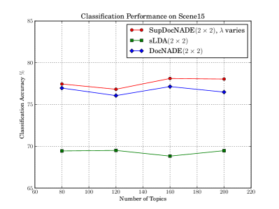
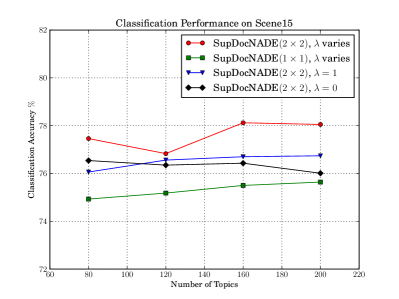
Figure 2: Classification performance comparison on Scene15 dataset. The left figure shows the performance comparison between SupDocNADE, DocNADE and sLDA. The figure on the right compares the performance of different variants of SupDocNADE.

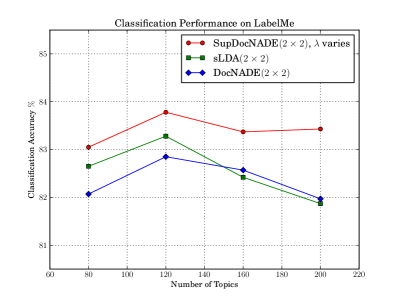
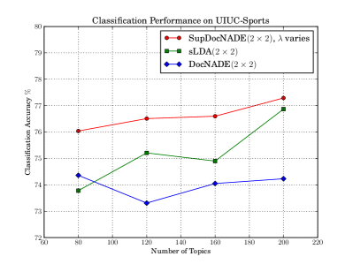
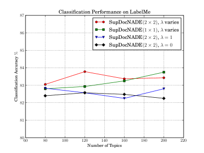
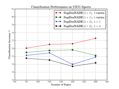
Figure 3: Classification performance comparison on LabelMe and UIUC-Sports datasets. In the top row, we compare the classification performance of SupDocNADE, DocNADE and sLDA. In the bottom row, we compare the performance between different variants of SupDocNADE. Results on LabelMe are on the left and results on UIUC-Sports are on the right.

We first test the classification performance of our method on the Scene15 dataset. Figure 2 illustrates the performance of all methods, for a varying number of topics. We observe that SupDocNADE outperforms sLDA by a large margin, while also improving over the orignal DocNADE model.

In Figure 2, we also compare SupDocNADE with other design choices for the model, such as performing purely generative ($\lambda=1$) or purely discriminative ($\lambda=0$) training, or ignoring spatial position information (i.e. using a single region, covering the whole image). We see that both using position information and tuning the weight $\lambda$ are important, with pure discriminative learning performing worse.

Wan et al. [14] also performed experiments on the Scene15 dataset using their hybrid topic/neural network model, but used a slightly different setup: they used 45 topics, a visual word vocabulary of size 200, a dense SIFT patch size of $32\times 32$ and a step size of 16. They also didn’t incorporate spatial position information using a spatial grid. When running SupDocNADE using this configuration, we obtain a classification accuracy of $73.36\%$, compared to $70.1\%$ for their model.

5.3.2 Simultaneous Classification and Annotation

We now look at the simultaneous image classification and annotation performance on LabelMe and UIUC-Sports datasets.

The classification results are illustrated in Figure 3. Similarly, we observe that SupDocNADE outperforms DocNADE and sLDA. Tuning the trade-off between generative and discriminative learning and exploiting position information is usually beneficial. There is just one exception, on LabelMe, with 200 hidden topic units, where using a $1\times 1$ grid slightly outperforms a $2\times 2$ grid.

As for image annotation, we computed the performance of our model with 200 topics. SupDocNADE obtains an $F$-measure of $43.87\%$ and $46.95\%$ on the LabelMe and UIUC-Sports datasets respectively. This is slightly superior to regular DocNADE, which obtains $43.32\%$ and $46.38\%$. Since code for performing image annotation using sLDA is not publicly available, we compare directly with the results found in the corresponding paper [2]. Wang et al. [2] report $F$-measures of $38.7\%$ and $35.0\%$ for sLDA, which is below SupDocNADE by a large margin.

We also compare with MMLDA [11], a max-margin formulation of LDA, that has been applied to image classification and annotation separately. The reported classification accuracy for MMLDA is $81.47\%$ (for LabelMe) and $74.65\%$ (for UIUC-Sports), which is less than SupDocNADE. As for annotation, $F$-measures of $46.64\%$ (for LabelMe) and $44.51\%$ (for UIUC-Sports) are reported, which is better than SupDocNADE on LabelMe but worse on UIUC-Sports. We should mention that MMLDA did not address the problem of simultaneously classifying and annotating images, these tasks being treated separately.

Figure 5 illustrates examples of correct and incorrect predictions made by SupDocNADE on the LabelMe dataset.

5.4 Visualization of Learned Representations

Since topic models are often used to interpret and explore the semantic structure of image data, we looked at how we could observe the structure learned by SupDocNADE.

We tried to extract the visual/annotation words that were most strongly associated with certain class labels within SupDocNADE. For example, given a class label street, which corresponds to a column $\mathbf{U}_{:,i}$ in matrix $\mathbf{U}$, we selected the top 3 topics (hidden units) having the largest connection weight in $\mathbf{U}_{:,i}$. Then, we averaged the columns of matrix $\mathbf{W}$ corresponding to these 3 hidden topics and selected the visual/annotation words with largest averaged weight connection. The results of this procedure for classes street, sailing, forest and highway is illustrated in Figure 4. To visualize the visual words, we show 16 image patches belonging to each visual word’s cluster, as extracted by $K$-means. The learned associations are intuitive: for example, the class street is associated with the annotation words “building”, “buildings”, “window”, “person walking” and “sky”, while the visual words showcase parts of buildings and windows.

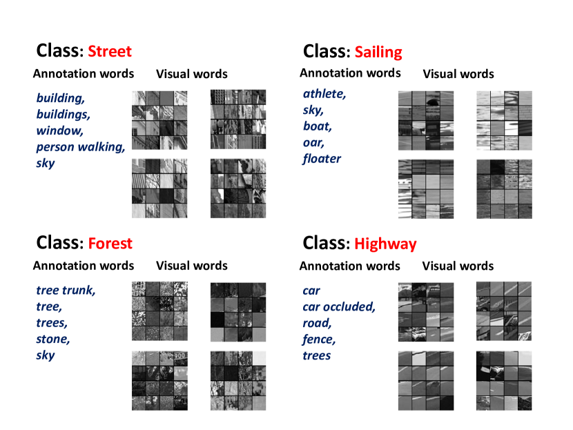
Figure 4: Visualization of learned representations. Class labels are colored in red. For each class, we list 4 visual words (each represented by 16 image patches) and 5 annotation words that are strongly associated with each class. See Section 5.4 for more details.

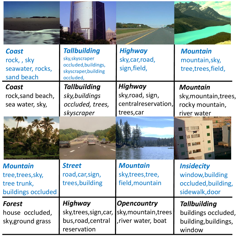
Figure 5: Predicted class and annotation by SupDocNADE on LabelMe dataset. We list some correctly (top row) and incorrectly (bottom row) classified images. The predicted (in blue) and ground-truth (in black) class labels and annotation words are presented under each image.

6 Conclusion and Discussion

In this paper, we proposed SupDocNADE, a supervised extension of DocNADE. Like all topic models, our model is trained to model the distribution of the bag of words representation of images and can extract a meaningful representation from it. Unlike most topic models however, the image representation is not modeled as a latent random variable in a model, but instead as the hidden layer of a neural network. While the resulting model might be less interpretable (as typical with neural networks), it has the advantage of not requiring any iterative, approximate inference procedure to compute an image’s representation. Our experiments confirm that SupDocNADE is a competitive approach for the classification and annotation of images.

References

- Blei et al. [2003] D. M. Blei, A. Y. Ng, and M. I. Jordan, “Latent dirichlet allocation,” JMLR, 2003.
- Wang et al. [2009] C. Wang, D. Blei, and F.-F. Li, “Simultaneous image classification and annotation,” in CVPR, 2009.
- Lazebnik et al. [2006] S. Lazebnik, C. Schmid, and J. Ponce, “Beyond bags of features: Spatial pyramid matching for recognizing natural scene categories,” in CVPR, 2006.
- Yang et al. [2009] J. Yang, K. Yu, Y. Gong, and T. Huang, “Linear spatial pyramid matching using sparse coding for image classification,” in CVPR, 2009.
- Tsai [2012] C.-F. Tsai, “Bag-of-words representation in image annotation: A review,” ISRN Artificial Intelligence, vol. 2012, 2012.
- Weston et al. [2010] J. Weston, S. Bengio, and N. Usunier, “Large scale image annotation: learning to rank with joint word-image embeddings,” Machine learning, 2010.
- Wu et al. [2009] Z. Wu, Q. Ke, J. Sun, and H.-Y. Shum, “A multi-sample, multi-tree approach to bag-of-words image representation for image retrieval,” in ICCV, 2009.
- Philbin et al. [2007] J. Philbin, O. Chum, M. Isard, J. Sivic, and A. Zisserman, “Object retrieval with large vocabularies and fast spatial matching,” in CVPR, 2007.
- David M. Blei [2007] J. D. M. David M. Blei, “Supervised topic models,” NIPS, 2007.
- Larochelle and Lauly [2012] H. Larochelle and S. Lauly, “A neural autoregressive topic model,” in NIPS 25, 2012.
- Wang and Mori [2011] Y. Wang and G. Mori, “Max-margin latent dirichlet allocation for image classification and annotation,” in BMVC, 2011.
- Bengio et al. [2012] Y. Bengio, A. Courville, and P. Vincent, “Representation learning: A review and new perspectives,” arXiv preprint arXiv:1206.5538, 2012.
- Salakhutdinov and Hinton [2009] R. Salakhutdinov and G. E. Hinton, “Replicated softmax: an undirected topic model,” NIPS, 2009.
- Wan et al. [2012] L. Wan, L. Zhu, and R. Fergus, “A hybrid neural network-latent topic model,” 2012.
- Bouchard et al. [2004] G. Bouchard, B. Triggs, et al., “The tradeoff between generative and discriminative classifiers,” in COMPSTAT, 2004.
- Glorot et al. [2011] X. Glorot, A. Bordes, and Y. Bengio, “Deep sparse rectifier networks,” in AISTATS, 2011.
- Nair and Hinton [2010] V. Nair and G. E. Hinton, “Rectified linear units improve restricted boltzmann machines,” in ICML, 2010.
- Russell et al. [2008] B. C. Russell, A. Torralba, K. P. Murphy, and W. T. Freeman, “Labelme: a database and web-based tool for image annotation,” IJCV, 2008.
- Li and Fei-Fei [2007] L.-J. Li and L. Fei-Fei, “What, where and who? classifying events by scene and object recognition,” in ICCV, 2007.