Two-mode effective interaction in a double-well condensate

Abstract

We investigate the origin of a disagreement between the two-mode model and the exact Gross-Pitaevskii dynamics applied to double-well systems. In general this model, even in its improved version, predicts a faster dynamics and underestimates the critical population imbalance separating Josephson and self-trapping regimes. We show that the source of this mismatch in the dynamics lies in the value of the on-site interaction energy parameter. Using simplified Thomas-Fermi densities, we find that the on-site energy parameter exhibits a linear dependence on the population imbalance, which is also confirmed by Gross-Pitaevskii simulations. When introducing this dependence in the two-mode equations of motion, we obtain a reduced interaction energy parameter which depends on the dimensionality of the system. The use of this new parameter significantly heals the disagreement in the dynamics and also produces better estimates of the critical imbalance.

Introduction.—Ultracold gases in double-well potentials exhibit a dynamics of matter at its most basic quantum level when both wells couple via a Bose-Josephson junction albiez05 . It is mostly interesting that the slow passage from non-self-trapped to self-trapped states, which is driven by a slow quench of the tunneling rate, is shown to obey the Kibble-Zurek mechanism for a continuous quantum phase transition Lee2009 . On the other hand, as a basic element of matter-wave interferometers, such a double-well configuration represents a good example of control of quantum coherence and entanglement in order to achieve high-precision metrology devices Schumm2005 . Being a widespread ingredient for modelling in a diversity of areas, such as quantum computing Strauch2008 and cosmology Neuenhahn2012 , it is of fundamental importance to achieve the best compromise between simplicity and accuracy in order to propose a theoretical description for these systems. In this respect, a seemingly good balance between both requirements is represented by the so-called two-mode (TM) model, which has been extensively studied in the last years smerzi97 ; ragh99 ; anan06 ; jia08 ; albiez05 ; mele11 ; abad11 . In particular, there is an active research in double-well systems doublewell which would greatly benefit from an accurate TM model. The dynamics in the TM model rests on assuming that the order parameter can be described as a superposition of localized on-site wave functions with time dependent coefficients. In 2005, both Josephson and self-trapping (ST) dynamics smerzi97 ; ragh99 were experimentally observed by Albiez et. al. albiez05 for large enough times so as to include several oscillations. They successfully measured the population imbalance and the phase difference between sites during the evolutions. We note that the TM model has in general predicted a sizable faster dynamics compared to both experiments and numerical simulations of the Gross Pitaevskii (GP) equations albiez05 ; mele11 ; abad11 ; gati2007 , in both Josephson and self-trapping regimes. The TM model predictions have also systematically provided an underestimated value of the critical imbalance for the transition between these regimes albiez05 ; mele11 ; abad11 ; gati2007 .

The main purpose of this letter is to put forward an explanation for such TM model disagreements. We revise the interaction term of the Gross-Pitaevskii equation and find that the interaction effect is overestimated by the TM model. Furthermore, for large number of particles we calculate an effective interaction energy parameter which reconciles the TM model with the numerical results.

The two-mode model.— The TM model ragh99 ; anan06 assumes the condensate wavefunction can be described as

$$\psi_{\mathrm{TM}}(r,t)=b_{R}(t)\,\psi_{R}({\bf r})+b_{L}(t)\,\psi_{L}({\bf r}),$$ (1)

where $\psi_{R}({\bf r})$ and $\psi_{L}({\bf r})$ are real, normalized to unity, localized on-site functions at the right and left wells, respectively. The complex time-dependent coefficients $b_{R}=\sqrt{n_{R}}e^{i\phi_{R}}$ and $b_{R}=\sqrt{n_{R}}e^{i\phi_{R}}$ verify $n_{R}+n_{L}=1$ being $n_{k}=N_{k}/N$, with $N_{k}$ the number of particles in the $k$-site, and $N$ the total number of particles. In order to obtain the TM dynamics one introduces the order parameter into the time-dependent GP equation,

$$i\hbar\frac{\partial\psi_{\mathrm{TM}}}{\partial t}=\left[-\frac{\hbar^{2}}{2m}{\bf\nabla}^{2}+V_{\rm{trap}}({\bf r})+g\,N\rho({\bf r},t)\right]\psi_{\mathrm{TM}}\,,$$ (2)

where $m$ is the atom mass, $V_{\rm{trap}}({\bf r})$ is the double-well potential, and $g=4\pi a\hbar^{2}/m$ is the coupling constant with $a$ the scattering length. The TM density $\rho({\bf r},t)$ takes the form,

$$\rho({\bf r},t)=n_{R}(t)\rho_{R}({\bf r})+n_{L}(t)\rho_{L}({\bf r})+2\mathrm{Re}(b_{R}^{*}b_{L})\psi_{R}({\bf r})\psi_{L}({\bf r}),$$ (3)

where we define the localized on-site densities $\rho_{k}({\bf r})=\psi_{k}^{2}({\bf r})$ with $k=R,L$. Multiplying Eq. (2) by both $\psi_{R}({\bf r})$ and $\psi_{L}({\bf r})$ and integrating the corresponding equations considering a symmetric double-well potential, one obtains the equations of motion

$$i\hbar\,\frac{db_{R}}{dt}=\, \varepsilon b_{R}-Jb_{L}+UN|b_{R}|^{2}b_{R}+IN\left[(b_{R}^{*}b_{L}+b_{R}b_{L}^{*})b_{L}\right.$$

$$\left.+|b_{L}|^{2}b_{R}\right]-FN\left[(b_{R}^{*}b_{L}+b_{R}b_{L}^{*})b_{R}+b_{L}\right],$$ (4)

$$i\hbar\,\frac{db_{L}}{dt}=\, \varepsilon b_{L}-Jb_{R}+UN|b_{L}|^{2}b_{L}+IN\left[(b_{L}^{*}b_{R}+b_{L}b_{R}^{*})b_{R}\right.$$

$$\left.+|b_{R}|^{2}b_{L}\right]-FN\left[(b_{L}^{*}b_{R}+b_{L}b_{R}^{*})b_{L}+b_{R}\right].$$ (5)

The on-site interaction energy parameter in $D$ dimensions is given by

$$U=g\int d^{D}{\bf r}\,\,\rho_{R}^{2}({\bf r})=g\int d^{D}{\bf r}\,\,\rho^{2}_{L}({\bf r}).$$ (6)

and the definition of the remaining parameters is given at the end of the letter, see Eqs. (21)–(24). In the equations of motion (4) and (5) all possible crossed terms involved in the TM model have been considered, in accordance with Ref. anan06 . In terms of the population imbalance $Z=n_{R}-n_{L}$ and phase difference $\phi=\phi_{L}-\phi_{R}$ the dynamical equations can be rewritten as,

$$\dot{Z} = -\sqrt{1-Z^{2}}\sin\phi+\gamma\,(1-Z^{2})\sin 2\phi\,,$$ (7)

$$\dot{\phi} = \Lambda Z+\left[\frac{Z}{\sqrt{1-Z^{2}}}\right]\cos\phi-\gamma\,Z(2+\cos 2\phi)$$ (8)

where $\Lambda=UN/{2K}$, $\gamma={IN}/{2K}$, and $K=J+FN$. The time derivatives have been expressed in units of $\hbar/2K$.

For the numerical simulations we consider a Bose-Einstein condensate of Rubidium atoms confined by the external trap $V_{\text{trap}}=\frac{1}{2}\,m\,\omega^{2}{\bf r}^{2}+V_{b}\,\exp(-x^{2}/\;\lambda_{b}^{2})$. We fix the trap frequency to $\omega/(2\pi)=77$ Hz, the number of particles to $N=10^{5}$, and for the barrier we choose $V_{b}=50\,\hbar\omega$ and a small width $\lambda_{b}=0.3\,l$, with $l=\sqrt{\hbar/(m\omega)}$ the harmonic oscillator length. In these conditions the TM parameters are $U=1.8993\times 10^{-4}\,\hbar\omega$, $J=1.2915\times 10^{-3}\hbar\omega$, $F=2.0245\times 10^{-8}\,\hbar\omega$, and $I=3.996\times 10^{-10}\,\hbar\omega$.

Modified model.— In order to identify the origin of the disagreement in the dynamics within the TM model, we investigate the effective potential felt by the system when the interaction term is included. To this aim, it is instructive to test the validity of the TM model by numerically calculating

$$U^{\mathrm{GP}}_{R}(t)=\frac{g}{n_{R}}\int d^{D}{\bf r}\,\,\rho_{\mathrm{GP}}({\bf r},t)\,\rho_{R}({\bf r}),$$ (9)

as a function of time, where $\rho_{\mathrm{GP}}({\bf r},t)$ is the full GP density normalized to unity, and compare it with $U^{\mathrm{\mathrm{TM}}}_{R}(t)=U+n_{L}(t)/n_{R}(t)I-2\mathrm{Re}(b_{R}^{*}b_{L})/n_{R}(t)F$ predicted by the TM dynamics. This has been obtained by replacing in (9) the GP density by the TM density given by Eq. (3). We note that $U^{\mathrm{\mathrm{TM}}}_{R}(t)\simeq U$ within a $10^{-4}$ relative error since the parameters $F$ and $I$ are four orders of magnitude smaller than $U$. In Fig. 1 we depict $1-U^{\mathrm{\mathrm{TM}}}_{R}(t)/U$ as a function of the population imbalance for two initial $Z(0)=\Delta N(0)/N$ values. These curves are almost vanishing within the error we have mentioned.

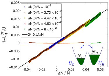
Figure 1: (color online) GP simulations of $1-U^{\mathrm{GP}}_{R}(t)/U$ (thick lines) and TM numerical calculations of $1-U^{\mathrm{\mathrm{TM}}}_{R}(t)/U$ (thin lines) as functions of the population imbalance for different initial imbalances $Z(0)=\Delta N(0)/N$. For all the evolutions the initial phase difference is $\phi(0)=0$. As a solid black line we have also depicted $1-U_{R}/U$ using $U_{R}$ given by Eq. (16). The inset shows a sketch of the double well potential with different populations.

Instead of the vanishing value predicted by the TM model in Fig. 1, the GP simulations of $1-U^{\mathrm{GP}}_{R}(t)/U$ exhibit an almost linear behavior with the imbalance $\Delta N/N$. The dispersion of the points is associated to the presence of sound waves.

Aiming at reproducing this linear behavior within a simple approach, we propose to take into account a more realistic density for describing the interacting term of the GP equation. The idea is to allow the localized on-site density to adopt the shape of what corresponds to the true acquired population at a given time. Thus, we propose to replace in the density defined by Eq. (3) the original $\psi_{R}({\bf r})$ and $\psi_{L}({\bf r})$ functions by unbalanced localized on-site $\psi^{\Delta N}_{R}({\bf r})$ and $\psi^{-\Delta N}_{L}({\bf r})$, respectively, corresponding to functions for artificial systems with a $N\pm\Delta N$ total number of particles with $\Delta N(t)=N_{R}(t)-N_{L}(t)$. These wavefunctions are normalized to unity and will be referred to as quasiestationary states, thus giving a density

$$\rho^{\Delta N}({\bf r},t)\simeq n_{R}(t)\rho^{\Delta N(t)}_{R}({\bf r})+n_{L}(t)\rho^{-\Delta N(t)}_{L}(\textbf{r})\\ +\left[b_{R}^{*}b_{L}+b_{R}b_{L}^{*}\right]\psi^{\Delta N(t)}_{R}(\textbf{r})\psi^{-\Delta N(t)}_{L}(\textbf{r}),$$ (10)

with $\rho_{R,L}^{\pm\Delta N}$ the corresponding localized on-site densities.

After performing such modifications the main correction is seen in Eq. (8), where the first term $\Lambda Z$ changes to,

$$N(U_{R}n_{R}-U_{L}n_{L})\frac{1}{2K}\,,$$ (11)

where $U_{R}=g\int d^{D}{\bf r}\,\,\rho^{\Delta N}_{R}({\bf r})\rho_{R}({\bf r})$ and $U_{L}=g\int d^{D}{\bf r}\,\,\rho^{-\Delta N}_{L}({\bf r})\rho_{L}({\bf r})$. To estimate $U_{R}$ we resort to the Thomas-Fermi (TF) approximation and assume that the barrier effect is just to cut the condensate into two halves without modifying its shape, note we have taken $\lambda_{b}<<R_{0}$. Thus, under these assumptions, the localized on the right site density in $D=3$ for a system with $N+\Delta N$ particles may be approximated by

$$\rho^{\Delta N}_{R}({\bf r})\simeq\frac{m\omega^{2}}{g(N+\Delta N)}\left(R_{\Delta N}^{2}-r^{2}\right)\Theta\left(R_{\Delta N}-r\right)\,\Theta(x),$$ (12)

where $\Theta(x)$ is the Heaviside function and $R_{\Delta N}$ denotes the corresponding TF radius. Then we may estimate,

$$U=g\int d^{3}{\bf r}\,\,\rho^{2}_{R}({\bf r})=g2\pi\int_{0}^{R_{0}}dr\,r^{2}\,\left[\frac{m\omega^{2}}{gN}(R_{0}^{2}-r^{2})\right]^{2}.$$ (13)

For evaluating $U_{R}$, we assume $\Delta N>0$, in which case $R_{0}<R_{\Delta N}$ because we are considering that the right site is more populated than the ground state. Thus, the upper limit in the integral in $r$ is $R_{0}$, giving

$$U_{R}=g2\pi\int_{0}^{R_{0}}\!\!drr^{2}\frac{m\omega^{2}}{gN}(R_{0}^{2}-r^{2})\,\frac{m\omega^{2}}{g(N+\Delta N)}(R_{\Delta N}^{2}-r^{2}).$$ (14)

After performing the integral and together with some algebra the quotient of both magnitudes is

$$\frac{U_{R}}{U}=\left[\frac{7}{4}\left(\frac{R_{\Delta N}}{R_{0}}\right)^{2}-\frac{3}{4}\right]\frac{N}{N+\Delta N}.$$ (15)

Making use of the normalization condition for the density in a three dimensional system, it is easy to verify that ${R_{\Delta N}}/{R_{0}}=[{(N+\Delta N)}/{N}]^{1/5}$, which inserted into the previous formulae yields,

$$\frac{U_{R}}{U}=\left[\frac{7}{4}\left(1+\frac{\Delta N}{N}\right)^{2/5}-\frac{3}{4}\right]\frac{1}{1+\frac{\Delta N}{N}}\simeq 1-\frac{3}{10}\frac{\Delta N}{N},$$ (16)

to first order approximation in ${\Delta N}/{N}$. It is interesting to note that the on-site parameter $U_{R}$ decreases when the population on the site increases, with respect to the stationary value, because the new normalized on-site density ($\rho^{\Delta N}_{R}({\bf r})$) spreads out over a wider region.

In Fig. 1 we have depicted $1-U_{R}/U$ with $U_{R}$ given by Eq. (16). Supposing that the density evolves in quasiestationary conditions we may approximate,

$$U^{\mathrm{GP}}_{R}(t) =\frac{g}{n_{R}}\int d^{D}{\bf r}\,\,\rho_{\mathrm{GP}}({\bf r},t)\rho_{R}({\bf r})$$

$$\simeq\frac{g}{n_{R}}\int d^{D}{\bf r}\,\,\rho^{\Delta N(t)}({\bf r},t)\,\rho_{R}({\bf r})$$

$$\simeq g\int d^{D}{\bf r}\,\,\rho^{\Delta N(t)}_{R}({\bf r})\rho_{R}({\bf r})=U_{R},$$ (17)

which is confirmed by the numerical results, as seen in Fig. 1.

On the other hand, proceeding in the same way on the left site but noting that in this case $R_{0}>R_{-\Delta N}$ one obtains,

$$\frac{U_{L}}{U}=\left[\frac{7}{4}-\frac{3}{4}\left(1-\frac{\Delta N}{N}\right)^{2/5}\right]\simeq 1+\frac{3}{10}\frac{\Delta N}{N}.$$ (18)

Then assuming the expressions Eqs. (16) and (18) are valid for every $\Delta N(t)$ during the evolution, we introduce them into the equation of motion for $\dot{\phi}$, Eq. (8), and in particular the first term turns to (cf. Eq. (11)):

$$\frac{U_{R}N_{R}-U_{L}N_{L}}{2K} =\frac{U_{R}}{2K}\left(\frac{N+\Delta N}{2}\right)-\frac{U_{L}}{2K}\left(\frac{N-\Delta N}{2}\right)$$

$$=\tilde{U}\,\frac{\Delta N}{2K}$$ (19)

with the effective interaction parameter $\tilde{U}=\frac{7}{10}U$. We note that the above approximation remains valid to second order in the imbalance. The same procedure can be applied in two and one dimension. The results are summarized in Table I and it is straightforward to prove that they are still valid for anisotropic traps. It is interesting to remark that even for very small population imbalance, where the on-site interaction energies are almost the same at the right and left sites ($U_{R}\simeq U_{L}\simeq U$), a sizeable difference (a factor $7/10$) between them and the effective $\tilde{U}$ parameter does exist.

Table 1: On-site interaction energy corrections for both right and left sites and the corresponding effective interaction energy parameter $\tilde{U}$ for systems in three, two and one dimensions.

Dimension	$U_{R}$	$U_{L}$	$\tilde{U}$
$D=3$	$(1-\frac{3}{10}\frac{\Delta N}{N})U$	$(1+\frac{3}{10}\frac{\Delta N}{N})U$	$\frac{7}{10}U$
$D=2$	$(1-\frac{1}{4}\frac{\Delta N}{N})U$	$(1+\frac{1}{4}\frac{\Delta N}{N})U$	$\frac{3}{4}U$
$D=1$	$(1-\frac{1}{6}\frac{\Delta N}{N})U$	$(1+\frac{1}{6}\frac{\Delta N}{N})U$	$\frac{5}{6}U$

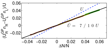
Figure 2: (color online) GP simulations of $(U^{\mathrm{GP}}_{R}n_{R}-U^{\mathrm{GP}}_{L}n_{L})/U$ as a function of the population imbalance for the same initial conditions as Fig. 1. The dashed line is the TM estimate while the solid one corresponds to the MTM model.

In Fig. 2 we depict $(U^{\mathrm{GP}}_{R}n_{R}-U^{\mathrm{GP}}_{L}n_{L})/U$ as a function of $\Delta N/N$ for several GP simulations. We also plot $(U_{R}n_{R}-U_{L}n_{L})/U$ using Eq. (19) as a solid line, and the TM prediction as a dashed line. It may be seen that the theoretical curve corresponding to the effective interaction parameter $\tilde{U}$ much better reproduces the numerical simulations.

On the other hand, we have also checked that when replacing $\psi^{\Delta N}_{L,R}({\bf r})$ in the definitions of the parameters $F$ and $I$, the corresponding numerical values change in less than one percent with respect to the original ones.

In view of the above results, we propose to modify the TM model by replacing the on-site interaction energy parameter U by the new constant parameter $\tilde{U}$ in the original equation of motion (8). This will be called the modified two-mode (MTM) model. In analogy to the TM model (disregarding the terms proportional to $\gamma$), the new equations of motion can be derived from the Hamiltonian,

$$H^{\mathrm{MTM}}=\frac{\tilde{\Lambda}}{2}Z^{2}-\sqrt{1-Z^{2}}\cos\phi\,,$$ (20)

where $\tilde{\Lambda}=\tilde{U}N/(2K)$, and $Z$ and $\phi$ are the canonical conjugate coordinates.

For our three dimensional system the renormalized parameters are $\tilde{U}=7/10\times 1.8993\times 10^{-4}\,\hbar\omega=1.3295\times 10^{-4}\,\hbar\omega$, and $\tilde{\Lambda}=2.004\times 10^{3}\,\hbar\omega$.

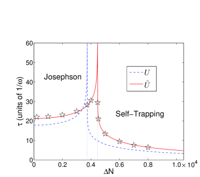
Figure 3: (color online) The time period (in units of $1/\omega$) as a function of the initial $\Delta N$ is depicted using the TM model (dashed line in blue), the MTM model (solid line in red ), and GP simulations (stars).

A very useful quantity for classifying the dynamics is the critical imbalance ($Z_{c}$), which separates initial conditions that evolve as either Josephson or self-trapping orbits. To appreciate one consequence of our finding, we compare this quantity using the bare on-site interaction parameter $\Delta N_{c}=NZ_{c}=2N/\sqrt{\Lambda}\simeq 3737$, and the renormalized one, which gives a larger estimate $\Delta N^{R}_{c}=2N/\sqrt{\tilde{\Lambda}}=\sqrt{10/7}\Delta N_{c}\simeq 4466$. By means of numerical simulations of the full GP equation, we have studied this transition and checked it effectively occurs around $\Delta N^{R}_{c}$.

In Fig. 3 we show the time period of the orbits using both approximate approaches (TM and MTM) and the GP simulations. It may be seen that the GP results are much better reproduced by the MTM approach. This is particularly evident in the asymptotic values corresponding to the critical imbalance where the period diverges. The TM curves are in accordance with previous results where the characteristic time was sizably underestimated with respect to both experimental and GP resultsalbiez05 ; mele11 . Only in a very narrow interval around the critical imbalance, the relation between the periods of the TM and the exact GP simulations is inverted, being the TM time period larger. On the other hand, the MTM model provides a consistent agreement along the full range of imbalance studied.

To illustrate the different dynamics we show in Fig. 4 the difference of particles between the sites as a function of time for different initial conditions. It may be seen that the MTM model gives a much more accurate dynamics than the TM model. Note that in the middle panel the MTM curve is almost superposed with the GP one.

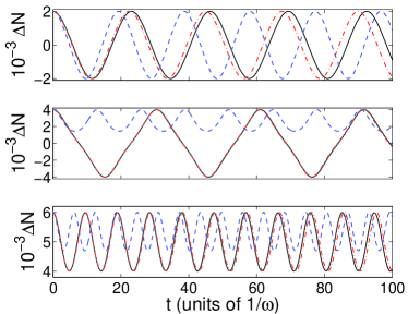
Figure 4: (color online) Time evolutions of GP simulations (solid black line), TM model (dashed blue line), and MTM model (dot-dashed red line) for the initial conditions $\Delta N(0)=2000$ (top panel), $\Delta N(0)=4000$ (middle panel), and $\Delta N(0)=6000$ (bottom panel).

Finally, we now complete the definitions of the TM model parameters,

$$\varepsilon=\int d^{D}{\bf r}\,\,\psi_{R}({\bf r})\left[-\frac{\hbar^{2}}{2m}{\bf\nabla}^{2}+V_{\rm{trap}}({\bf r})\right]\psi_{R}({\bf r})$$ (21)

$$J=-\int d^{D}{\bf r}\,\,\psi_{R}({\bf r})\left[-\frac{\hbar^{2}}{2m}{\bf\nabla}^{2}+V_{\rm{trap}}({\bf r})\right]\psi_{L}({\bf r})$$ (22)

$$F=-\,g\int d^{D}{\bf r}\,\,\psi_{R}^{3}({\bf r})\psi_{L}({\bf r})$$ (23)

$$I=g\int d^{D}{\bf r}\,\,\psi_{R}^{2}({\bf r})\,\psi_{L}^{2}({\bf r}),$$ (24)

where, due to the symmetry, we have chosen arbitrarily the right well for performing the calculations.

Conclusions.—By considering a more realistic effective interaction we were able to construct a more accurate two-mode model. Such a model is obtained by only replacing the on-site interaction energy parameter by a reduced one, with simple scaling factors depending on dimensionality. We have found that our modified model reproduces much better the particle dynamics predicted by GP simulations in a double well potential, both in the Josephson and self-trapping regimes.

This study can be extended to multiple well systems, in particular to optical lattices with a high number of particles per site anker05 ; jezek12 .

DMJ and HMC acknowledge CONICET for financial support under Grant No. PIP 11420090100243 and PIP 11420100100083, respectively. PC acknowledges support from CONICET and UBA through Grants No. PIP 0546 and UBACYT 01/K156.

References

- (1) M. Albiez, R. Gati, J. Fölling, S. Hunsmann, M. Cristiani, and M. K. Oberthaler, Phys. Rev. Lett. 95, 010402 (2005); M. Albiez, PhD Thesis, University of Heidelberg (2005).
- (2) C. Lee, Phys. Rev. Lett. 102 070401 (2009); C. Lee, J. Huang, H. Deng, H. Dai, and J. Xu, Front. Phys. 7 109 (2012).
- (3) T. Schumm, S. Hofferberth, L. M. Andersson, S. Wildermuth, S. Groth, I. Bar-Joseph, J. Schmiedmayer, and P. Krüger, Nature Phys. 1 57 (2005).
- (4) F. W. Strauch, M. Edwards, E. Tiesinga, C. Williams, and C. W. Clark, Phys. Rev. A 77, 050304(R) (2008).
- (5) C. Neuenhahn, A. Polkovnikov, and F. Marquardt, Phys. Rev. Lett. 109 085304 (2012).
- (6) A. Smerzi, S. Fantoni, S. Giovanazzi, and S. R. Shenoy, Phys. Rev. Lett. 79, 4950 (1997).
- (7) S. Raghavan, A. Smerzi, S. Fantoni, and S. R. Shenoy, Phys. Rev. A 59, 620 (1999).
- (8) D. Ananikian and T. Bergeman, Phys. Rev. A 73, 013604 (2006).
- (9) Xin Yan Jia, Wei Dong Li, and J. Q. Liang, Phys. Rev. A 78, 023613 (2008).
- (10) M. Melé-Messeguer, B. Juliá-Díaz, M. Guilleumas, A. Polls and A. Sanpera, New J. Phys. 13, 033012 (2011).
- (11) M. Abad, M. Guilleumas, R. Mayol, M. Pi, and D. M. Jezek, Europhys. Lett. 94, 10004 (2011).
- (12) H. Hennig, D. Witthaut, and D. K. Campbell, Phys. Rev. A 86, 051604(R) (2012); X.-F. Zhou, S.-L. Zhang, Z.-W. Zhou, B. A. Malomed, and H. Pu, ibid. 85, 023603 (2012); M. A. García-March, D. R. Dounas-Frazer, and L. D. Carr, ibid. 83, 043612 (2011); Q. Zhou, J. V. Porto, and S. Das Sarma, ibid. 84, 031607 (2011); M. Abad, M. Guilleumas, R. Mayol, M. Pi, and D. M. Jezek, ibid. 84, 035601 (2011); T. Zibold, E. Nicklas, C. Gross, and M. K. Oberthaler, Phys. Rev. Lett. 105, 204101 (2010); L. J. LeBlanc, A. B. Bardon, J. McKeever, M. H. T. Extavour, D. Jervis, J. H. Thywissen, F. Piazza, and A. Smerzi, ibid. 106, 025302 (2011);
- (13) R. Gati and M. K. Oberthaler, J. Phys B: At. Mol. Opt. Phys. 40. R61 (2007).
- (14) D. M. Jezek and H. M. Cataldo, to be published.
- (15) Th. Anker, M. Albiez, R. Gati, S. Hunsmann, B. Eiermann, A. Trombettoni, and M. K. Oberthaler, Phys. Rev. Lett. 94, 020403 (2005).