Abstract

In this paper we propose a generalization of a class of Gaussian Semiparametric Estimators (GSE) of the fractional differencing parameter for long-range dependent multivariate time series. We generalize a known GSE-type estimator by introducing some modifications at the objective function level regarding the process’ spectral density matrix estimator. We study large sample properties of the estimator without assuming Gaussianity as well as hypothesis testing. The class of models considered here satisfies simple conditions on the spectral density function, restricted to a small neighborhood of the zero frequency. This includes, but is not limited to, the class of VARFIMA models. A simulation study to assess the finite sample properties of the proposed estimator is presented and supports its competitiveness. We also present an empirical application to an exchange rate data.
Keywords: Multivariate processes; Long-range dependence; Semiparametric estimation; VARFIMA processes; Asymptotic theory.
Mathematical Subject Classification (2010). Primary 62H12, 62F12, 62M10, 60G10, 62M15.

1 Introduction

Semiparametric estimation of the fractional differencing parameter in multivariate long-range dependent time series has seen growing attention in the last few years (see, for instance, Lobato, 1999, Andersen et al., 2003 and Chiriac and Voev, 2011). The first attempt to develop the theory of semiparametric estimation in the context of univariate long-range dependent time series seems to point back to late 80’s with the work of Künsch (1987), which proposed a local Whittle-type estimator. The idea of the estimator is to locally model the behavior of the spectral density function in long-range dependent time series by locally approximating the time-domain Gaussian likelihood near the origin. These estimators comprehend the widely applied class of Gaussian Semiparametric Estimators (GSE, for short). The asymptotic theory of the particular estimator proposed in Künsch (1987) was challenging and posed some real theoretical difficulties in its development given the non-linear definition of the estimator. The first asymptotic results were presented in Robinson (1995b) and later further studied in Velasco (1999), Phillips and Shimotsu (2004), among others. Several variants also emerged (Hurvich and Chen, 2000, Shimotsu and Phillips, 2005, among others).

The estimation of the fractional differencing parameter in long-range dependent time series started focusing on the fully parametric case. In the univariate case, the asymptotic theory of Whittle’s estimator was fully described in the work of Fox and Taqqu (1986) and Giraitis and Surgailis (1990), while the asymptotic theory of the exact maximum likelihood estimator was established by Dahlhaus (1989) and later extended to the multivariate case by Hosoya (1997), although Sowell (1989) has studied the method in the context of VARFIMA processes before. The computational cost of the exact maximum likelihood procedure in the multivariate case is high. A relatively fast approximation is studied in Luceño (1996) and, more recently, in Tsay (2010), both in the context of VARFIMA processes.

Fully parametric methods present some important asymptotic properties such as efficiency, $n^{1/2}$-consistency and asymptotic normality under the correct specification of the parametric model. The main criticism to the method comes from its inconsistency under misspecification of the underlying parametric structure and from the crucial role played by Gaussianity assumptions in the asymptotic theory (but see Giraitis and Surgailis, 1990), both contestable in real life applications. In this direction, the semiparametric approach presents many advantages over the parametric one, such as less distributional requirements, robustness against short-run dependencies and more efficiency compared to the latter. Another important advantage of the semiparametric approach is that Gaussianity is usually not assumed in the asymptotic theory.

The first rigorous treatment of a multivariate semiparametric estimator was given in Robinson (1995a). Lobato (1999) analyzes a two-step GSE based on a simple local approximation of the spectral density function in the neighborhood of the origin and derive its (Gaussian) asymptotic distribution. Shimotsu (2007) analyzes another multivariate GSE by considering a refinement of the local approximation considered in Lobato (1999) and, extending the techniques in Robinson (1995b), shows its consistency and asymptotic normality. Shimotsu (2007) also considers a “single-step” version of Lobato (1999)’s estimator and shows its consistency and asymptotic normality. The work of Shimotsu (2007) has been recently extended to cover non-stationary multivariate long-range dependent processes in Nielsen (2011).

In this paper we are interested in semiparametric estimation of the fractional differencing parameter on multivariate long-range dependent processes. The idea is to generalize the “single-step” version of Lobato (1999)’s GSE considered in Shimotsu (2007) by substituting the periodogram function, applied in defining the estimator’s objective function, by an arbitrary estimator of the spectral density. Although a useful tool in spectral analysis, it is well-known that the periodogram is an ill-behaved inconsistent estimator of the spectral density. Seen as a random variable, it does not even converge to a random variable at all (cf. Grenander, 1951) being considered by some authors “an extremely poor (if not useless) estimate of the spectral density function” (Priestley, 1981, p.420). A natural question is can we improve the performance of the GSE estimator by considering spectral density estimators other than the periodogram? Answering this question is the main focus of our study.

Our theoretical contribution is focused on large sample properties of the proposed estimator considering different classes of spectral density estimators. First we consider objective functions with the periodogram substituted by consistent estimators of the spectral density function. We show the consistency of the GSE obtained under the same conditions in the process as considered in Shimotsu (2007). Second, we relax the consistency condition by considering spectral density estimators satisfying certain mild moment conditions and show the consistency of the related estimator. Third we examine the asymptotic normality of the proposed estimator under a certain mild regularity condition on the spectral density estimator and under the same assumptions as in Shimotsu (2007). The limiting distribution turns out to be the same as the estimator considered in Shimotsu (2007). We also consider hypothesis testing related problems. Gaussianity is nowhere assumed in the asymptotic theory.

To exemplify the use and to assess the finite sample performance of the proposed estimator, we consider the particular cases where the smoothed periodogram and the tapered periodogram are applied as spectral density estimators. We perform a Monte Carlo simulation study based on the resulting GSE and compare it to the same estimator based on the periodogram itself. We also apply the estimators to a real data set.

The paper is organized as follows. In the next section we consider some preliminary results and definitions necessary to this work and introduce the proposed estimator. In Section 3, we study the consistency of the proposed estimator while in Section 4 we derive the estimator’s asymptotic distribution. In Section 5 we present a Monte Carlo simulation study in order to assess the estimator’s finite sample performance and compare it to the “single-step” version of Lobato’s estimator considered in Shimotsu (2007). The real data application is presented in Section 6 and the conclusions in Section 7. For the presentation sake, the proofs of the results in this work are presented in Appendix A.

2 Preliminaries

Let $\{\boldsymbol{X}_{t}\}_{t=0}^{\infty}$ be a weakly stationary $q$-dimensional process and let $f$ denote the spectral density matrix function of $\boldsymbol{X}_{\!t}$, so that

$$\mathds{E}\big{[}\big{(}\boldsymbol{X}_{\!t}-\mathds{E}(\boldsymbol{X}_{\!t})\big{)}\big{(}\boldsymbol{X}_{\!t+h}-\mathds{E}(\boldsymbol{X}_{\!t})\big{)}^{\prime}\big{]}=\int_{-\pi}^{\pi}\mathrm{e}^{\mathrm{i}h\lambda}f(\lambda)d\lambda,$$

for $h\in\mathds{N}^{\ast}:=\mathds{N}\!\setminus\!\{0\}$. In Lobato (1999), the author considers processes for which the spectral density matrix satisfies the following local approximation

$$f(\lambda)\,\sim\operatorname*{\mathrm{diag}}_{i\in\{1,\cdots,q\}}\{\lambda^{-d_{i}}\}\ G_{0}\!\!\!\operatorname*{\mathrm{diag}}_{i\in\{1,\cdots,q\}}\{\lambda^{-d_{i}}\},\quad\mbox{ as }\lambda\rightarrow 0^{+},$$ (2.1)

where $d_{i}\in(-0.5,0.5)$, $i=1,\cdots,q$ and $G_{0}$ is a symmetric positive definite real matrix.

Although specification (2.1) is somewhat general, as noted in Lobato (1999), several fractionally integrated models satisfy this condition. Each coordinate process of $\{\boldsymbol{X}_{t}\}_{t=0}^{\infty}$ exhibits long-range dependence whenever the respective parameter $d_{i}>0$, in the sense that the respective (unidimensional) spectral density function satisfies $f(\lambda)\sim K\lambda^{-2d_{i}}$, as $\lambda\rightarrow 0^{+}$, for some constant $K>0$ and $i\in\{1,\cdots,q\}$.

Let

$$w_{n}(\lambda)\vcentcolon=\frac{1}{\sqrt{2\pi n}}\sum_{t=1}^{n}\boldsymbol{X}_{\!t}\mathrm{e}^{\mathrm{i}t\lambda}\quad\mbox{ and }\quad I_{n}(\lambda)\vcentcolon=w_{n}(\lambda)\overline{w_{n}(\lambda)}^{\,\,\prime}$$ (2.2)

be the discrete Fourier transform and the periodogram of $\boldsymbol{X}_{\!t}$ at $\lambda$, respectively, where $\overline{A}^{\,\,\prime}$ denotes the conjugate transpose of a complex matrix $A$.

From the local form of the spectral density function (2.1) and the frequency domain Gaussian log-likelihood localized in the neighborhood of zero, Lobato (1999) introduces a two-step Gaussian semiparametric estimator for the parameter $\boldsymbol{d}=(d_{1},\cdots,d_{q})^{\prime}$, henceforth denoted by $\widetilde{\boldsymbol{d}}$. The estimator is a two-step optimization procedure based on the objective function

$$\widetilde{S}(\boldsymbol{d}):=\log\big{(}\det\widetilde{G}(\boldsymbol{d})\big{)}-2\sum_{k=1}^{q}d_{k}\frac{1}{m}\sum_{j=1}^{m}\log(\lambda_{j}),$$ (2.3)

where $\lambda_{j}:=2\pi j/n$, for $j=1,\cdots,m$, are the Fourier frequencies, $m=o(n)$, with $n$ denoting the sample size, and

$$\widetilde{G}(\boldsymbol{d}):=\frac{1}{m}\sum_{j=1}^{m}\mathrm{Re}\bigg{[}\operatorname*{\mathrm{diag}}_{i\in\{1,\cdots,q\}}\{\lambda_{j}^{-d_{i}}\}I_{n}(\lambda_{j})\operatorname*{\mathrm{diag}}_{i\in\{1,\cdots,q\}}\{\lambda_{j}^{-d_{i}}\}\bigg{]},$$ (2.4)

where, as usual, $\mathrm{Re}[z]$ denotes the real part of $z\in\mathds{C}$. For $i\in\{1,\cdots,q\}$, let $d_{i}^{Q}$ denote the univariate quasi-maximum likelihood estimate (QMLE) given in Robinson (1995b) obtained from the $i$-th coordinate process. The first step is to obtain an initial estimate of $\boldsymbol{d}$ by calculating the univariate QMLE for each coordinate process. Let $\boldsymbol{d}^{Q}:=(d_{1}^{Q},\cdots,d_{q}^{Q})^{\prime}$. The final estimate is obtained by calculating

$$\widetilde{\boldsymbol{d}}:=\boldsymbol{d}^{Q}-\bigg{(}\frac{\partial^{2}\widetilde{S}(\boldsymbol{d})}{\partial\boldsymbol{d}\partial{\boldsymbol{d}}^{\prime}}\bigg{|}_{\boldsymbol{d}=\boldsymbol{d}^{Q}}\bigg{)}^{\!\!-1}\!\bigg{(}\frac{\partial\widetilde{S}(\boldsymbol{d})}{\partial\boldsymbol{d}}\bigg{|}_{\boldsymbol{d}=\boldsymbol{d}^{Q}}\bigg{)}.$$ (2.5)

Naturally, in this case the estimator of the matrix $G_{0}$ in (2.1) is just $\widetilde{G}:=\widetilde{G}(\widetilde{\boldsymbol{d}})$.

Under some mild conditions, Lobato (1999) shows that, when the spectral density function follows (2.1), the estimator (2.5) satisfies $m^{1/2}(\widetilde{\boldsymbol{d}}-\boldsymbol{d})\overset{d}{\longrightarrow}2\big{(}G_{0}\odot G_{0}^{-1}+\mathrm{I}_{q}\big{)}$, as $m$ tends to infinity, where $\mathrm{I}_{q}$ is the $q\times q$ identity matrix and $\odot$ denotes the Hadamard produtct.

Notice that one can consider the same estimator based on the objective function (2.3) as a “single-step” estimator by solving the $q$-dimensional optimization problem

$$\widetilde{\boldsymbol{d}}:=\underset{\boldsymbol{d}\in\Theta}{\arg\min}\{\widetilde{S}(\boldsymbol{d})\},$$ (2.6)

where $\Theta$ is the parameter space, usually some subset of $(-0.5,0.5)^{q}$. Estimator (2.6) was considered in details in Shimotsu (2007). Arguably, a two-step procedure like the one necessary to obtain $\widetilde{\boldsymbol{d}}$ in (2.5) is computationally faster than a direct $q$-dimensional optimization procedure as (2.6). In the late 90’s, a direct multidimensional optimization procedure could be troublesome considering the computational resources available for the general public at the epoch. Nowadays, however, with the recent advances in computer sciences and the development of faster CPU’s, a direct optimization procedure such as (2.6) represents no difficulty in practice.

Shimotsu (2007) considered a more refined local approximation for the spectral density matrix, namely

$$f(\lambda_{j})\sim\Lambda_{j}(\boldsymbol{d})G\overline{\Lambda_{j}(\boldsymbol{d})}^{\,\,\prime},\quad\mbox{where}\quad\Lambda_{j}(\boldsymbol{d})=\operatorname*{\mathrm{diag}}_{k\in\{1,\cdots,q\}}\{\Lambda_{j}^{(k)}(\boldsymbol{d})\}\quad\mbox{and}\quad\Lambda_{j}^{(k)}(\boldsymbol{d})=\lambda_{j}^{-d_{k}}\mathrm{e}^{\mathrm{i}(\pi-\lambda_{j})d_{k}/2},$$ (2.7)

and studied the asymptotic behavior of (2.6) under (2.7). Under some mild conditions, the author showed the consistency and asymptotical normality of the estimator (2.6) under (2.7) even though, in this case, the estimator is based on the misspecified model (2.1).

Now let $\{\boldsymbol{X}_{t}\}_{t=0}^{\infty}$ be a weakly stationary $q$-dimensional process and let $f$ denote its spectral density matrix function satisfying (2.7). Let $f_{n}$ denote an arbitrary estimator of $f$ based on the observations $\boldsymbol{X}_{1},\cdots,\boldsymbol{X}_{n}$. Consider the objective function

$$S(\boldsymbol{d}):=\log\big{(}\det\big{\{}\widehat{G}(\boldsymbol{d})\big{\}}\big{)}-2\sum_{k=1}^{q}d_{k}\frac{1}{m}\sum_{j=1}^{m}\log(\lambda_{j}),$$ (2.8)

with

$$\widehat{G}(\boldsymbol{d}):=\frac{1}{m}\sum_{j=1}^{m}\mathrm{Re}\bigg{[}\operatorname*{\mathrm{diag}}_{i\in\{1,\cdots,q\}}\{\lambda_{j}^{-d_{i}}\}f_{n}(\lambda_{j})\operatorname*{\mathrm{diag}}_{i\in\{1,\cdots,q\}}\{\lambda_{j}^{-d_{i}}\}\bigg{]},$$ (2.9)

where, again, $\lambda_{j}:=2\pi j/n$, for $j=1,\cdots,m$ and $m=o(n)$. Notice that (2.9) is just (2.4) with $f_{n}$ substituting the periodogram $I_{n}$. Let us define the general estimator

$$\widehat{\boldsymbol{d}}:=\underset{\boldsymbol{d}\in\Theta}{\arg\min}\{S(\boldsymbol{d})\},$$ (2.10)

where $\Theta$ denotes the space of admissible estimates, usually a subset of $(-0.5,0.5)^{q}$. In this work we are interested in studying the asymptotic behavior and finite sample performance of the estimator (2.10) as a function of $f_{n}$. The estimator (2.10) is a refinement of Lobato (1999) and a generalization of the results on the estimator (2.6) presented in Shimotsu (2007). Our asymptotic study is divided in two main cases. First, we consider the case where $f_{n}$ is an arbitrary consistent estimator of the spectral density $f$. Secondly, we consider the case where $f_{n}$ is an arbitrary estimator of $f$ satisfying a certain moment condition. The intersection between the two cases is not empty, as we shall discuss later on.

3 Asymptotic Theory: Consistency

Let $\{\boldsymbol{X}_{\!t}\}_{t=0}^{\infty}$ be a weakly stationary $q$-dimensional process and let $f=(f_{rs})_{r,s=1}^{q}$ be its spectral density matrix satisfying (2.1) for a real, symmetric and positive definite matrix $G_{0}=(G_{0}^{rs})_{r,s=1}^{q}$. Let $\boldsymbol{d}_{0}=(d_{1}^{0},\cdots,d_{q}^{0})^{\prime}$ be the true fractional differencing vector parameter. As usual, the sup-norm is denoted by $\|\cdot\|_{\infty}$ and to simplify the notation, we shall denote the $r$-th row and the $s$-th column of a matrix $M$ by $(M)_{r\boldsymbol{\cdot}}$ and $(M)_{\boldsymbol{\cdot}s}$, respectively. Before proceed with the asymptotic theory, let us state the necessary conditions for the consistency of the estimator.

• Assumption A1. As $\lambda\rightarrow 0^{+}$,

  $$f_{rs}(\lambda)=\mathrm{e}^{\mathrm{i}\pi(d_{r}^{0}-d_{s}^{0})/2}G_{0}^{rs}\lambda^{-d_{r}^{0}-d_{s}^{0}}+o(\lambda^{-d_{r}^{0}-d_{s}^{0}}),\quad\mbox{ for all }\,r,s=1,\cdots,q.$$

• Assumption A2. The process $\{\boldsymbol{X}_{t}\}_{t=0}^{\infty}$ is a causal linear process, that is,

  $$\boldsymbol{X}_{\!t}-\mathds{E}(\boldsymbol{X}_{\!t})=\sum_{k=0}^{\infty}A_{k}\boldsymbol{\varepsilon}_{t-k},\quad\mbox{with}\quad\sum_{k=0}^{\infty}\big{\|}A_{k}\big{\|}_{\infty}^{2}<\infty,$$ (3.1)

  where the innovation process $\{\boldsymbol{\varepsilon}_{t}\}_{t\in\mathds{Z}}$ is a (not necessarily uncorrelated) square integrable martingale difference, in the sense that

  $$\mathds{E}(\boldsymbol{\varepsilon}_{t}|\mathscr{F}_{t-1})=0\quad\mbox{ and }\quad\mathds{E}(\boldsymbol{\varepsilon}_{t}\boldsymbol{\varepsilon}_{t}^{\prime}|\mathscr{F}_{t-1})=\mathrm{I}_{q}\quad\mbox{a.s.,}$$

  for all $t\in\mathds{Z}$, where $\mathscr{F}_{t}$ denotes the $\sigma$-field generated by $\{\boldsymbol{\varepsilon}_{s},s\leq t\}$. Also assume that there exist a random variable $\xi$ and a constant $K>0$ such that $\mathds{E}(\xi^{2})<\infty$ and $\mathds{P}\big{(}\|\boldsymbol{\varepsilon}_{t}\|_{\infty}^{2}>\eta\big{)}\leq K\mathds{P}(\xi^{2}>\eta)$, for all $\eta>0$.

• Assumption A3. With $\{A_{k}\}_{k\in\mathds{N}}$ given in (3.1), define the function

  $$A(\lambda)\vcentcolon=\sum_{k=0}^{\infty}A_{k}\mathrm{e}^{\mathrm{i}k\lambda}.$$ (3.2)

  In a neighborhood $(0,\delta)$, $\delta>0$, of the origin, we assume that $A$ is differentiable and

  $$\frac{\partial}{\partial\lambda}\big{(}\overline{A(\lambda)}^{\,\,\prime}\big{)}_{r\boldsymbol{\cdot}}=O\Big{(}\lambda^{-1}\Big{\|}\big{(}\overline{A(\lambda)}^{\,\,\prime}\big{)}_{r\boldsymbol{\cdot}}\Big{\|}_{\infty}\Big{)},\quad\mbox{as }\lambda\rightarrow 0^{+}.$$

• Assumption A4. As $n\rightarrow\infty$,

  $$\frac{1}{m}+\frac{m}{n}\longrightarrow 0.$$

Remark 3.1.

Assumptions A1-A4 are the multivariate extensions of those in Robinson (1995b) considered in Shimotsu (2007). Assumption A1 describes the true spectral density matrix behavior at the origin. Replacing $\mathrm{e}^{\mathrm{i}\pi(d_{r}^{0}-d_{s}^{0})/2}$ by $\mathrm{e}^{\mathrm{i}(\pi-\lambda)(d_{r}^{0}-d_{s}^{0})/2}$ makes asymptotically no difference, since $\lim_{\lambda\rightarrow 0^{+}}\mathrm{e}^{\mathrm{i}\lambda}-1=0$. Assumption A2 regards the behavior of the innovation process which is assumed to be a not necessarily uncorrelated square integrable martingale difference uniformly dominated in probability by a square integrable random variable. Assumption A3 is a regularity condition often imposed in the parametric case as, for instance, in Fox and Taqqu (1986) and Giraitis and Surgailis (1990). Assumption A4 is minimal but necessary since $m$ must go to infinity for consistency, but must do so slower than $n$ in view of Assumption A1.

Assumptions A1-A4 are local ones and only regard the spectral density behavior at the vicinities of the origin. Outside a small neighborhood of the origin, no assumption on the spectral density is made (except, of course, for the integrability of the spectral density, implied by the weak stationarity of the process).

For $\beta\in[0,1]$, let $f_{n}$ be a $n^{\beta}$-consistent estimator of the spectral density function for all $\boldsymbol{d}_{0}\in B$ where $B$ is a closed subset of $\mathds{R}^{q}$. Since the spectral density matrix of the process $\{\boldsymbol{X}_{\!t}\}_{t=0}^{\infty}$ is unbounded at the zero frequency when $d_{k}^{0}\in(0,0.5)$, for some $k\in\{1,\cdots,q\}$, there is no hope in finding a consistent estimator for it in this situation. Let

$$\Omega_{\beta}\vcentcolon=\bigg{[}-\frac{\beta}{2},0\bigg{]}^{q}\bigcap\bigg{(}-\frac{1}{2},0\bigg{]}^{q}\bigcap B\subseteq\bigg{(}-\frac{1}{2},0\bigg{]}^{q},$$ (3.3)

Next we consider the estimator (2.10) with $\Theta=\Omega_{\beta}$, that is

$$\widehat{\boldsymbol{d}}:=\underset{\boldsymbol{d}\in\Omega_{\beta}}{\arg\min}\{S(\boldsymbol{d})\}.$$ (3.4)

In the next theorem we establish the consistency of (3.4) under Assumptions A1-A4 considering an $n^{\beta}$-consistent spectral density function estimator. For the sake of a better presentation, the proofs of all results in the paper are postponed to Appendix A.

Theorem 3.1.

Let $\{\boldsymbol{X}_{\!t}\}_{t=0}^{\infty}$ be a weakly stationary $q$-dimensional process and let $f$ be its spectral density matrix. Let $f_{n}$ be a $n^{\beta}$-consistent estimator of $f$ for all $\boldsymbol{d}_{0}\in B\subseteq\mathds{R}^{q}$, for $\beta\in[0,1]$, and let $\widehat{\boldsymbol{d}}$ be as in (3.4). Assume that Assumptions A1-A4 hold and let $\boldsymbol{d}_{0}\in\Omega_{\beta}$. Then, $\widehat{\boldsymbol{d}}\overset{\mathds{P}}{-\!\!\!\longrightarrow}\boldsymbol{d}_{0}$, as $n\rightarrow\infty$.

We now study the problem of relaxing the $n^{\beta}$-consistency of the spectral density estimator $f_{n}$ assumed in Theorem 3.1. We consider the class of estimators $f_{n}:=(f_{n}^{rs})_{r,s=1}^{q}$ satisfying, for $1\leq u<v\leq m$,

$$\max_{r,s\in\{1,\cdots,q\}}\bigg{\{}\sum_{j=u}^{v}\mathrm{e}^{\mathrm{i}(\lambda_{j}-\pi)(d_{r}^{0}-d_{s}^{0})/2}\lambda_{j}^{d^{0}_{r}+d^{0}_{s}}f_{n}^{rs}(\lambda_{j})-G_{0}^{rs}\bigg{\}}=o_{\mathds{P}}(1)$$ (3.5)

for $\boldsymbol{d}_{0}\in\Theta\subseteq(-0.5,0.5)^{q}$. A relatively simpler condition implying (3.5) is as follows:

Lemma 3.1.

Let $\{\boldsymbol{X}_{\!t}\}_{t=0}^{\infty}$ be a weakly stationary $q$-dimensional process and let $f$ be its spectral density matrix and assume that assumptions A1-A4 hold. Let $f_{n}$ be an estimator of $f$ satisfying for all $r,s\in\{1,\cdots,q\}$ and $\boldsymbol{d}_{0}\in\Theta$,

$$\mathds{E}\Big{(}\lambda_{j}^{d_{r}^{0}+d_{s}^{0}}\Big{|}f_{n}^{rs}(\lambda_{j})-\big{(}A(\lambda_{j})\big{)}_{r\boldsymbol{\cdot}}I_{\boldsymbol{\varepsilon}}(\lambda_{j})\big{(}\overline{A(\lambda_{j})}^{\,\,\prime}\big{)}_{\boldsymbol{\cdot}s}\Big{|}\Big{)}\>=o(1),\quad\mbox{ as }\>n\rightarrow\infty,$$ (3.6)

where $A$ is given by (3.2) and $I_{\boldsymbol{\varepsilon}}$ denotes the periodogram function associated to $\{\boldsymbol{\varepsilon}_{t}\}_{t\in\mathds{Z}}$, that is,

$$I_{\boldsymbol{\varepsilon}}(\lambda):=w_{\boldsymbol{\varepsilon}}(\lambda)\overline{w_{\boldsymbol{\varepsilon}}(\lambda)}^{\,\,\prime},\qquad\text{where}\qquad w_{\boldsymbol{\varepsilon}}(\lambda)\vcentcolon=\frac{1}{\sqrt{2\pi n}}\sum_{t=1}^{n}\boldsymbol{\varepsilon}_{t}\mathrm{e}^{\mathrm{i}t\lambda}.$$

Then, for $1\leq u<v\leq m$,

$$\max_{r,s\in\{1,\cdots,q\}}\bigg{\{}\sum_{j=u}^{v}\mathrm{e}^{\mathrm{i}(\lambda_{j}-\pi)(d_{r}^{0}-d_{s}^{0})/2}\lambda_{j}^{d^{0}_{r}+d^{0}_{s}}f_{n}^{rs}(\lambda_{j})-G_{0}^{rs}\bigg{\}}=\mathscr{A}_{uv}+\mathscr{B}_{uv},$$

where $\mathscr{A}_{uv}$ and $\mathscr{B}_{uv}$ satisfy

$$\mathds{E}\big{(}|\mathscr{A}_{uv}|\big{)}=o(v-u+1)\qquad\mbox{ and }\qquad\max_{1\leq u<v\leq m}\big{\{}\big{|}v^{-1}\mathscr{B}_{uv}\big{|}\big{\}}=o_{\mathds{P}}(1).$$

Thus, (3.5) holds.

The class of estimators satisfying (3.5) is non-empty since, for instance, both, the ordinary and the tapered periodogram satisfy (3.6) in the form $O(j^{-1/2}\log(j+1))$ (see lemma 1 in Shimotsu, 2007 and Section 5.3 below). Condition (3.5) is just slightly more general than (3.6). For the periodogram, (3.5) can be seen directly as well, but it is more involved (see lemma 1 in Shimotsu, 2007). Condition (3.5) plays a crucial role in replacing the $n^{\beta}$-consistency assumed in Theorem 3.1, as we shall see later. From an asymptotic point of view, (3.5) is a sufficient condition to prove the consistency of $\widehat{\boldsymbol{d}}$ under Assumptions A1-A4. This is the content of the next theorem.

Theorem 3.2.

Let $\{\boldsymbol{X}_{\!t}\}_{t=0}^{\infty}$ be a weakly stationary $q$-dimensional process and let $f$ be its spectral density matrix. Let $f_{n}$ be an estimator of $f$ satisfying (3.5), for all $r,s\in\{1,\cdots,q\}$ and $\boldsymbol{d}_{0}\in\Theta$ and consider the estimator $\widehat{\boldsymbol{d}}$ given by (2.10) based on $f_{n}$. Assume that assumptions A1-A4 hold. Then $\widehat{\boldsymbol{d}}\overset{\mathds{P}}{-\!\!\!\longrightarrow}\boldsymbol{d}_{0}$, as $n$ tends to infinity.

4 Asymptotic Distribution and Hypothesis Testing

Let $\{\boldsymbol{X}_{\!t}\}_{t=0}^{\infty}$ be a weakly stationary $q$-dimensional process, let $f=(f_{rs})_{r,s=1}^{q}$ be its spectral density matrix. Suppose that $f$ satisfies (2.1) for a real, symmetric and positive definite matrix $G_{0}=(G_{0}^{rs})_{r,s=1}^{q}$. Let $\boldsymbol{d}_{0}=(d_{1}^{0},\cdots,d_{q}^{0})^{\prime}$ be the true fractional differencing vector parameter. Assume that the following assumptions are satisfied

• Assumption B1. For $\alpha\in(0,2\,]$ and $r,s\in\{1,\cdots,q\}$,

  $$f_{rs}(\lambda)=\mathrm{e}^{\mathrm{i}(\pi-\lambda)(d_{r}^{0}-d_{s}^{0})/2}\lambda^{-d_{r}^{0}-d_{s}^{0}}G_{0}^{rs}+O(\lambda^{-d_{r}^{0}-d_{s}^{0}+\alpha}),\,\,\text{ as }\lambda\rightarrow 0^{+}.$$

• Assumption B2. Assumption A2 holds and the process $\{\boldsymbol{\varepsilon}_{t}\}_{t\in\mathds{Z}}$ has finite fourth moment.

• Assumption B3. Assumption A3 holds.

• Assumption B4. For any $\delta>0$,

  $$\frac{1}{m}+\frac{m^{1+2\alpha}\log(m)^{2}}{n^{2\alpha}}+\frac{\log(n)}{m^{\delta}}\longrightarrow 0,\,\,\text{ as }n\rightarrow\infty.$$

• Assumption B5. There exists a finite real matrix $M$ such that

  $$\Lambda_{j}(\boldsymbol{d}_{0})^{-1}A(\lambda_{j})=M+o(1),\,\,\text{ as }\lambda_{j}\rightarrow 0.$$

Remark 4.1.

Assumption B1 is a smoothness condition on the behavior of the spectral density function near the origin. It is slightly stronger than Assumption A1 and is often imposed in spectral analysis. Assumption B2 imposes that the process $\{\boldsymbol{X}_{t}\}_{t=0}^{\infty}$ is linear with finite fourth moment. This restriction in the innovation process is necessary since the proof of Theorem 4.1 depends on a CLT-type result for a martingale difference sequence defined as a quadratic form involving $\{\boldsymbol{\varepsilon}_{t}\}_{t\in\mathds{Z}}$, which must have finite variance. Assumption B4 is the same as assumption 4’ in Shimotsu (2007). In particular, it implies that $(m/n)^{b}=o\big{(}m^{-\frac{b}{2\alpha}}\,\log(m)^{-\frac{b}{\alpha}}\big{)}$, for $b\neq 0$. Assumption B5 is the same as assumption 5’ in Shimotsu (2007) and it is a mild regularity condition in the degree of approximation of $A(\lambda_{j})$ by $\Lambda_{j}(\boldsymbol{d}_{0})$. It is satisfied by general VARFIMA processes.

Lemma 4.1.

Let $\{\boldsymbol{X}_{\!t}\}_{t=0}^{\infty}$ be a weakly stationary $q$-dimensional process. Let $f$ be its spectral density matrix and assume that assumptions B1-B5 hold, with B4 holding for $\alpha=1$. Let $f_{n}$ be an estimator of $f$ satisfying

$$\max_{1\leq v\leq m}\bigg{\{}\sum_{j=1}^{v}\Big{[}f_{n}^{rs}(\lambda_{j})-\big{(}A(\lambda_{j})\big{)}_{r\boldsymbol{\cdot}}I_{\boldsymbol{\varepsilon}}(\lambda_{j})\big{(}\overline{A(\lambda_{j})}^{\,\,\prime}\big{)}_{\boldsymbol{\cdot}s}\Big{]}\bigg{\}}=o_{\mathds{P}}\bigg{(}\frac{m^{2}}{n^{1+|d_{r}^{0}+d_{s}^{0}|}}\bigg{)},$$ (4.1)

for all $r,s\in\{1,\cdots,q\}$ and $\boldsymbol{d}_{0}\in\Theta$. Then,

• $$\max_{1\leq v\leq m}\bigg{\{}\max_{r,s}\!\bigg{\{}\!\sum_{j=1}^{v}\lambda_{j}^{d_{r}^{0}+d_{s}^{0}}\Big{[}f_{n}^{rs}(\lambda_{j})-\big{(}A(\lambda_{j})\big{)}_{r\boldsymbol{\cdot}}I_{\boldsymbol{\varepsilon}}(\lambda_{j})\big{(}\overline{A(\lambda_{j})}^{\,\,\prime}\big{)}_{\boldsymbol{\cdot}s}\Big{]}\!\bigg{\}}\bigg{\}}=o_{\mathds{P}}\bigg{(}\frac{\sqrt{m}}{\log(m)}\bigg{)};$$ (4.2)

• $$\max_{1\leq v\leq m}\bigg{\{}\max_{r,s}\!\bigg{\{}\sum_{j=1}^{v}\lambda_{j}^{d_{r}^{0}+d_{s}^{0}}f_{n}^{rs}(\lambda_{j})-\mathrm{e}^{\mathrm{i}(\pi-\lambda_{j})(d_{r}^{0}-d_{s}^{0})/2}G_{0}^{rs}\bigg{\}}\bigg{\}}=O_{\mathds{P}}\bigg{(}\frac{m^{\alpha+1}}{n^{\alpha}}+\sqrt{m}\log(m)\bigg{)}.$$ (4.3)

The next theorem establishes the asymptotic normality of estimator (2.10) under Assumptions B1-B5 considering the class of estimators $f_{n}$ satisfying (4.1). To make the presentation simpler, let us define the matrices

$$\mathcal{E}_{0}:=\operatorname*{\mathrm{diag}}_{k\in\{1,\cdots,q\}}\Big{\{}\mathrm{e}^{\mathrm{i}\pi d_{k}^{0}/2}\Big{\}},\quad\mathcal{G}_{0}:=\mathrm{Re}\big{[}\mathcal{E}_{0}G_{0}\overline{\mathcal{E}_{0}}^{\,\,\prime}\big{]}\ \ \mbox{ and }\ \ \quad g_{0}:=\mathrm{Im}\big{[}\mathcal{E}_{0}G_{0}\overline{\mathcal{E}_{0}}^{\,\,\prime}\big{]}.$$ (4.4)

Theorem 4.1.

Let $\{\boldsymbol{X}_{\!t}\}_{t=0}^{\infty}$ be a weakly stationary $q$-dimensional process, let $f$ be its spectral density matrix and assume that assumptions B1-B5 hold, with B4 holding for $\alpha=1$. Let $f_{n}$ be an estimator of $f$ satisfying (4.1), for all $r,s\in\{1,\cdots,q\}$ and $\boldsymbol{d}_{0}\in\Theta$. If $\widehat{\boldsymbol{d}}\overset{\mathds{P}}{\longrightarrow}\boldsymbol{d}_{0}$, for $\boldsymbol{d}_{0}\in\Theta$, then

$$m^{1/2}(\widehat{\boldsymbol{d}}-\boldsymbol{d}_{0})\overset{d}{-\!\!\!\longrightarrow}N(\boldsymbol{0},\Omega),$$

as $n$ tends to infinity, where

$$\Omega\vcentcolon=\frac{1}{2}\big{(}\mathcal{G}_{0}\odot\mathcal{G}_{0}^{-1}+\mathrm{I}_{q}\big{)}^{-1}\Sigma\ \big{(}\mathcal{G}_{0}\odot\mathcal{G}_{0}^{-1}+\mathrm{I}_{q}\big{)}^{-1},$$

with

$$\Sigma:=\mathcal{G}_{0}\odot\mathcal{G}_{0}^{-1}+\mathrm{I}_{q}+(\mathcal{G}_{0}^{-1}g_{0}\mathcal{G}_{0}^{-1})\odot g_{0}-(\mathcal{G}_{0}^{-1}g_{0})\odot(\mathcal{G}_{0}^{-1}g_{0})^{\prime},$$

and $\mathrm{I}_{q}$ the $q\times q$ identity matrix. Furthermore, $\widehat{G}(\widehat{\boldsymbol{d}})\overset{\mathds{P}}{\longrightarrow}\mathcal{G}_{0}$.

Remark 4.2.

A careful inspection on the proof of Theorem 4.1 reveals that it suffices that the estimator $f_{n}$ satisfies parts (a) and (b) of Lemma 4.1 in order to it hold, which are implied by (4.1).

The asymptotic variance-covariance matrix $\Omega$ takes a cumbersome form. A simple case occurs when $d_{1}^{0}=\cdots=d_{q}^{0}$ in which case $\mathcal{G}_{0}=G_{0}$ and $\Omega=2[G_{0}\odot G_{0}^{-1}-\mathrm{I}_{q}]$, the variance-covariance matrix of the limiting distribution of Lobato (1999)’s two-step estimator. Also, by Theorem 4.1, $\widehat{G}(\widehat{\boldsymbol{d}})$ is not a consistent estimator of $G_{0}$. However, since the $(r,s)$-th element of $\mathcal{G}_{0}$ is $\mathcal{G}_{0}^{rs}=\cos\big{(}\pi(d_{r}^{0}-d_{s}^{0})/2\big{)}G_{0}^{rs}$, a consistent estimator of the matrix $G_{0}$ under the hypothesis of Theorem 4.1 is

$$\widehat{\mathrm{G}}:=\tau(\widehat{\boldsymbol{d}})\odot\widehat{G}(\widehat{\boldsymbol{d}}),\qquad\mbox{ where }\qquad\tau(\widehat{\boldsymbol{d}})_{rs}:=\frac{1}{\cos\big{(}\pi(\hat{d}_{r}-\hat{d}_{s})/2\big{)}}\,.$$

This result allows for hypothesis testing. First, let $\widehat{\Omega}$ denote the matrix defined in the same way as $\Omega$ is defined in Theorem 4.1, but with $\widehat{\mathrm{G}}$ in place of $G_{0}$. It follows that, under the hypothesis of Theorem 4.1, $\widehat{\Omega}\overset{\mathds{P}}{\longrightarrow}\Omega$. Let $0<s\leq q$ and let $R$ be a $s\times q$ non-zero real matrix and $\boldsymbol{\nu}\in\mathds{R}^{s}$. Consider testing a set of $s$ (independent) linear restrictions on $\boldsymbol{d}_{0}$ of the form

$$H_{0}:R\boldsymbol{d}_{0}=\boldsymbol{\nu}\quad\mbox{versus}\quad H_{a}:R\boldsymbol{d}_{0}\neq\boldsymbol{\nu}.$$

Assuming the conditions of Theorem 4.1, under $H_{0}$ the test statistics

$$T:=m(R\widehat{\boldsymbol{d}}-\boldsymbol{\nu})^{\prime}\big{(}R\widehat{\Omega}R^{\prime}\big{)}^{-1}(R\widehat{\boldsymbol{d}}-\boldsymbol{\nu})$$ (4.5)

is asymptotically distributed as a $\chi_{s}^{2}$ distribution. As particular cases we have: testing the process for a common fractional differencing parameter, in which case $R=(\mathrm{I}_{q-1}\vdots\boldsymbol{0})-(\boldsymbol{0}\vdots\mathrm{I}_{q-1})$ with dimension $q-1\times q$ and $\boldsymbol{\nu}=\boldsymbol{0}$, where $\boldsymbol{0}$ is a vector composed by $q-1$ zeroes; testing if the process is $I(0)$, in which case $R=\mathrm{I}_{q}$ and $\boldsymbol{\nu}$ is a vector of $q$ zeroes. Notice that in the particular case where $f_{n}$ is the periodogram $I_{n}$, and thus, $\widehat{\boldsymbol{d}}=\widetilde{\boldsymbol{d}}$, (4.5) is also valid by theorem 3 in Shimotsu (2007).

5 Simulation Study

In this section we present a Monte Carlo simulation study to assess the finite sample performance of the estimator (2.10) and compare it to (2.6). In order to do that, we apply the tapered periodogram and the smoothed periodogram as the spectral density estimator $f_{n}$ on (2.9). Before presenting the simulation study, let us recall some facts on the the smoothed and tapered periodograms.

5.1 The Smoothed Periodogram

Let $\{\boldsymbol{X}_{\!t}\}_{t=0}^{\infty}$ be a weakly stationary $q$-dimensional process. Let $W_{n}(\cdot)\vcentcolon=\big{(}W_{n}^{ij}(\cdot)\big{)}_{i,j=1}^{q}$ be an array of functions (called weight functions) and $\{\ell(k)\}_{k\in\mathds{N}}$ be an increasing sequence of positive integers. For a Fourier frequency $\lambda_{j}$, we define the smoothed periodogram of $\boldsymbol{X}_{\!t}$ by

$$f_{n}(\lambda_{j})\vcentcolon=\sum_{|k|\leq\ell(n)}W_{n}(k)\odot w_{n}(\lambda_{j+k})\overline{w_{n}(\lambda_{j+k})}^{\,\,\prime},$$ (5.1)

where $w_{n}(\cdot)$ is given by (2.2) and $\odot$ denotes the Hadamard product. If, for some $j$ and $k$, $\lambda_{j+k}\notin[-\pi,\pi]$, we take $w_{n}$ as having period $2\pi$. In practice, at zero frequency, we use a slightly different estimative, namely,

$$f_{n}(0)\vcentcolon=\mathrm{Re}\!\bigg{[}W_{n}(0)\odot w_{n}(\lambda_{1})\overline{w_{n}(\lambda_{1})}^{\,\,\prime}+2\sum_{k=1}^{\ell(n)}W_{n}(k)\odot w_{n}(\lambda_{k+1})\overline{w_{n}(\lambda_{k+1})}^{\,\,\prime}\bigg{]}.$$

When the process $\{\boldsymbol{X}_{\!t}\}_{t=0}^{\infty}$ is long-range dependent, its spectral density present a pole at zero frequency, so that some authors take the summation in (5.1) restricted to $k\neq-j$. In finite samples, however, $w_{n}(0)$ is always well defined since the process is finite with probability one. More details on the smoothed periodogram can be found, for instance, in Priestley (1981) and references therein.

The smoothed periodogram as defined in (5.1) is a multivariate extension of the univariate smoothed periodogram. The use of the Hadamard product in the definition allows the use of different weight functions across different components of the process, accommodating, in this manner, the necessity often observed in practice of modeling different spectral density characteristics, including cross spectrum ones, with different weight functions. We refrain from discussing the different types of weight functions in the literature, since the subject is present in most textbooks. See, for instance, Priestley (1981), where a broad account of different weight functions, their properties and further references can be found.

In the asymptotic theory, we are only interested in sequences $\{\ell(k)\}_{k\in\mathds{N}}$ and weight functions $W_{n}(\cdot)$ satisfying

• Assumption C1. $1/\ell(n)+\ell(n)/n\longrightarrow 0$, as $n$ tends to infinity;

• Assumption C2. $W_{n}^{ij}(k)=W_{n}^{ij}(-k)$ and $W_{n}^{ij}(k)\geq 0$, for all $k$;

• Assumption C3. $\sum_{|k|\leq\ell(n)}W_{n}^{ij}(k)=1$;

• Assumption C4. $\sum_{|k|\leq\ell(n)}W_{n}^{ij}(k)^{2}\longrightarrow 0$, as $n$ tends to infinity.

Under Assumptions C1-C4, the smoothed periodogram is an $n^{1/2}$-consistent estimator of the spectral density matrix for all $\boldsymbol{d}\in[-0.5,0]^{q}$. Assumptions C1-C4 are standard ones in the asymptotic theory of the smoothed periodogram (see, for instance, Priestley, 1981). Assumption C1 controls the convergence rate of the sequence $\{\ell(k)\}_{k\in\mathds{N}}$ with respect to $n$. Assumptions C2-C3 impose that the weight functions must be non-negative symmetric functions and that the sequences $\big{\{}W_{n}^{ij}(k)\big{\}}_{k=-\ell(n)}^{\ell(n)}$ form a convex sequence of coefficients for each $n$, $i$ and $j$. Assumption C4 is just a mild technical condition for the consistency of the estimator.

Since the smoothed periodogram (under Assumptions C1-C4) is an $n^{1/2}$-consistent estimator of the spectral density function for $\boldsymbol{d}_{0}\in B:=[-1/2,0]^{q}$, Theorem 3.1 applies and we conclude that the estimator (3.4) (under Assumptions A1-A4) is consistent for all $\boldsymbol{d}_{0}\in\Omega_{1/2}=[-1/4,0]^{q}$. To this moment, we were not able to establish the consistency of the estimator (2.10) based on the smoothed periodogram via Theorem 3.2 nor its asymptotic normality via Theorem 4.1. However, there is empirical evidence (as we shall show later) that this is indeed the case.

5.2 The Tapered Periodogram

The main idea on the tapered periodogram is to obtain a decrease on the asymptotic bias by tapering the data before calculating the periodogram of the series. This is specially helpful in the case of long-range dependent time series. See, for instance, Priestley (1981) and Hurvich and Beltrão (1993).

Let $\{\boldsymbol{X}_{\!t}\}_{t=0}^{\infty}$ be a weakly stationary $q$-dimensional process. For $i\in\{1,\cdots,q\}$, let $h_{i}:[0,1]\rightarrow\mathds{R}$ be a collection of functions. Consider the vector of functions $L_{n}(\cdot):=\big{(}L_{n}^{i}(\cdot)\big{)}_{i=1}^{q}$ defined as $L_{n}^{i}(\lambda):=h_{i}\big{(}\lambda/n\big{)}$ and let

$$\ S_{n}(\lambda):=\Bigg{(}\frac{L_{n}^{i}(\lambda)}{\sqrt{\sum_{t=1}^{n}L_{n}^{i}(t)^{2}}}\Bigg{)}_{i=1}^{q}.$$

The tapered periodogram $I_{T}(\lambda;n)$ of $\{\boldsymbol{X}_{\!t}\}_{t=1}^{n}$ is then defined by setting

$$I_{T}(\lambda;n):=w_{T}(\lambda;n)\overline{w_{T}(\lambda;n)}^{\,\,\prime},\quad\mbox{ where }\quad w_{T}(\lambda;n):=\frac{1}{\sqrt{2\pi}}\sum_{t=1}^{n}S_{n}(t)\odot\boldsymbol{X}_{\!t}\mathrm{e}^{-it\lambda}.$$ (5.2)

We shall assume the following:

• Assumption D. The tapering functions $h_{i}$ are of bounded variation and $H_{i}:=\int_{0}^{1}h_{i}^{2}(x)dx>0$, for all $i\in\{1,\cdots,q\}.$

The tapered periodogram is not a consistent estimator of the spectral density function, since the reduction on the bias induces, in this case, an augmentation of the variance. Just as the ordinary periodogram, the increase in the variance can be dealt by smoothing the tapered periodogram in order to obtain a consistent estimator of the spectral density function in the case $\boldsymbol{d}\in(-0.5,0)$ (see, for instance, the recent work of Fryzlewicz, Nason and von Sachs, 2008). Usually, a good performance of the tapered periodogram is obtained through tapering functions which decay faster than the Féjer’s kernel. For more information on the choices of taper functions, see Priestley (1981), Dahlhaus (1983), Hurvich and Beltrão (1993), Fryzlewicz, Nason and von Sachs (2008) and references therein.

Under Assumption D, $\sum_{t=1}^{n}L_{n}^{i}(t)^{2}\sim nH_{i}$ (cf. Fryzlewicz, Nason and von Sachs, 2008) so that $I_{T}(\lambda;n)=O\big{(}I_{n}(\lambda)\big{)}$. This allows to show that the estimator (2.10) based on the tapered periodogram is also consistent and asymptotically normally distributed. These are the contents of the next Corollaries.

Corollary 5.1.

Let $\{\boldsymbol{X}_{\!t}\}_{t=0}^{\infty}$ be a weakly stationary $q$-dimensional process with spectral density $f$ satisfying Assumptions A1-A4. Let $f_{n}$ be the tapered periodogram defined in (5.2) satisfying Assumption D. For $\boldsymbol{d}_{0}\in\Theta$, consider the estimator $\widehat{\boldsymbol{d}}$ based on $f_{n}$, as given in (2.10). Then, $\widehat{\boldsymbol{d}}\overset{\mathds{P}}{-\!\!\!\longrightarrow}\boldsymbol{d}_{0}$, as $n$ tends to infinity.

Corollary 5.2.

Let $\{\boldsymbol{X}_{\!t}\}_{t=0}^{\infty}$ be a weakly stationary $q$-dimensional process with spectral density $f$ satisfying Assumptions B1-B5, with B4 holding for $\alpha=1$. Let $f_{n}$ be the tapered periodogram given in (5.2) satisfying Assumption D. For $\boldsymbol{d}_{0}\in\Theta$, consider the estimator $\widehat{\boldsymbol{d}}$ based on $f_{n}$, as given in (2.10). Then, for $\boldsymbol{d}_{0}\in\Theta$,

$$m^{1/2}(\widehat{\boldsymbol{d}}-\boldsymbol{d}_{0})\overset{d}{-\!\!\!\longrightarrow}N(\boldsymbol{0},\Omega),$$

as $n$ tends to infinity, with $\Omega$ as given in Theorem 4.1.

5.3 Simulation Results

Recall that the class of VARFIMA$(p,\boldsymbol{d},q)$ processes comprehend $q$-dimensional stationary processes $\{\boldsymbol{X}_{t}\}_{t\in\mathds{Z}}$ which satisfy the difference equations

$$\boldsymbol{\Phi}({\cal B})\,\mathrm{diag}\big{\{}(1-{\cal B})^{\boldsymbol{d}}\big{\}}\big{(}\boldsymbol{X}_{t}-\mathds{E}(\boldsymbol{X}_{t})\big{)}=\boldsymbol{\Theta}({\cal B})\boldsymbol{\varepsilon}_{t},$$

where $\cal B$ is the backward shift operator, $\{\boldsymbol{\varepsilon}_{t}\}_{t\in\mathds{Z}}$ is an $m$-dimensional stationary process (the innovation process), $\boldsymbol{\Phi}({\cal B})$ and $\boldsymbol{\Theta}({\cal B})$ are $m\times m$ matrices in ${\cal B}$, given by the equations

$$\boldsymbol{\Phi}({\cal B})=\sum_{\ell=0}^{p}\boldsymbol{\phi}_{\ell}{\cal B}^{\ell}\,\,\,\,\mbox{and}\,\,\,\,\boldsymbol{\Theta}({\cal B})=\sum_{r=0}^{q}\boldsymbol{\theta}_{r}{\cal B}^{r},$$

assumed to have no common roots, where $\boldsymbol{\phi}_{1},\cdots,\boldsymbol{\phi}_{p},\boldsymbol{\theta}_{1},\cdots,\boldsymbol{\theta}_{q}$ are real $m\times m$ matrices and $\boldsymbol{\phi}_{0}=\boldsymbol{\theta}_{0}=\boldsymbol{I}_{m\times m}$, the $m\times m$ identity matrix.

The simulation study is based on bidimensional Gaussian VARFIMA$(0,\boldsymbol{d},0)$ time series (i.i.d. innovation process) of sample size $n=1,000$ for four different pairs of the parameter $\boldsymbol{d}$ and (within component) correlation $\rho\in\{0,0.3,0.6,0.8\}$. A total of 1,000 replications is performed for each set of parameters. The time series are generated by the widely applied method of truncating the multidimensional infinite moving average representation of the process. The truncation point is fixed at 50,000 for all cases. The goal is the estimation of the parameter $\boldsymbol{d}$. To do that, we consider the estimator (2.10) with the tapered and the smoothed periodogram as the spectral density matrix estimator $f_{n}$. For the tapered periodogram, we apply the cosine-bell tapering function, namely,

$$h_{i}(u)=\left\{\begin{array}[]{cc}\frac{1}{2}\big{[}1-\cos(2\pi u)\big{]},&\mbox{ if }\ 0\leq u\leq 1/2,\vspace{.2cm}\\ h_{i}(1-u),&\mbox{ if }\ 1/2<u\leq 1,\end{array}\right.\quad\mbox{ for all }i=1,2.$$

The resulting estimator is denoted by TLOB. The cosine-bell taper is often applied as tapering function in applications as, for instance, in Hurvich and Ray (1995), Velasco (1999) and Olbermann et al. (2006). For the smoothed periodogram, we apply the so-called Bartlett’s weights for all spectral density components, namely

$$W_{n}^{ij}(k):=\frac{\sin^{2}\big{(}\ell(n)\lambda_{k}/2\big{)}}{n\ell(n)\sin^{2}(\lambda_{k}/2)},\quad\mbox{ for all }i,j=1,2.$$

We consider the smoothed periodogram with and without the restriction $k\neq-j$ in (5.1) and the resulting estimator are denoted by SLOB and $SLOB^{\ast}$, respectively. We also apply, for comparison purposes, the estimator given in (2.6), denoted by LOB. The specific truncation point of the smoothed periodogram function is of the form $\ell(n):=\ell(n,\beta)=\lfloor n^{\beta}\rfloor$, for $\beta\in\{0.7,0.9\}$ while the truncation point of the objective function (2.8) is of the form $m:=m(n,\alpha)=\lfloor n^{\alpha}\rfloor$, for $\alpha\in\{0.65,0.85\}$ for all estimators. All simulations were performed by using the computational resources of the (Brazilian) Center of Super Computing (CESUP-UFRGS). The routines were all implemented in FORTRAN 95 language optimized with OpenMP directives for parallel computing.

Table 5.1 and 5.2 report the simulation results for $\boldsymbol{d}\in\big{\{}(0.2,0.3),(0.1,0.4),(0.3,0.4),(0.1,0.3)\big{\}}$. Presented are the estimated values (mean), their standard deviations (st.d.) and the mean square error of the estimates (mse).

Table 5.1: Simulation results for the estimators SLOB, $SLOB^{\ast}$, TLOB and LOB in Gaussian VARFIMA$(0,\boldsymbol{d},0)$ processes. Presented are the estimated values (mean), their standard deviation (st.d) and mean square error of the estimates (mse).

$\rho$	Method	$\beta$	$\hat{d}_{i}$	$\boldsymbol{d}=(0.1,0.4)$						$\boldsymbol{d}=(0.2,0.3)$
				$\alpha=0.65$			$\alpha=0.85$			$\alpha=0.65$			$\alpha=0.85$
				mean	st.d.	mse	mean	st.d.	mse	mean	st.d.	mse	mean	st.d.	mse
$0$	SLOB	0.7	$\hat{d}_{1}$	0.1024	0.0543	0.0030	0.0954	0.0268	0.0007	0.2081	0.0569	0.0033	0.1944	0.0277	0.0008
			$\hat{d}_{2}$	0.4470	0.0788	0.0084	0.4138	0.0401	0.0018	0.3167	0.0644	0.0044	0.2999	0.0321	0.0010
		0.9	$\hat{d}_{1}$	0.1044	0.0560	0.0032	0.0953	0.0267	0.0007	0.2085	0.0564	0.0033	0.1923	0.0269	0.0008
			$\hat{d}_{2}$	0.4233	0.0624	0.0044	0.3950	0.0306	0.0010	0.3080	0.0580	0.0034	0.2919	0.0289	0.0009
	SLOB$\phantom{B}{}^{\ast}$	0.7	$\hat{d}_{1}$	0.0922	0.0549	0.0031	0.0917	0.0270	0.0008	0.1923	0.0567	0.0033	0.1884	0.0275	0.0009
			$\hat{d}_{2}$	0.3840	0.0618	0.0041	0.3855	0.0308	0.0012	0.2789	0.0594	0.0040	0.2849	0.0298	0.0011
		0.9	$\hat{d}_{1}$	0.0977	0.0573	0.0033	0.0931	0.0270	0.0008	0.1992	0.0578	0.0033	0.1891	0.0271	0.0009
			$\hat{d}_{2}$	0.3900	0.0607	0.0038	0.3815	0.0295	0.0012	0.2871	0.0599	0.0038	0.2844	0.0292	0.0011
	LOB	-	$\hat{d}_{1}$	0.1051	0.0579	0.0034	0.0955	0.0271	0.0008	0.2070	0.0580	0.0034	0.1915	0.0271	0.0008
			$\hat{d}_{2}$	0.3957	0.0606	0.0037	0.3822	0.0292	0.0012	0.2938	0.0602	0.0037	0.2860	0.0291	0.0010
	TLOB	-	$\hat{d}_{1}$	0.1056	0.0785	0.0062	0.0956	0.0377	0.0014	0.2075	0.0783	0.0062	0.1916	0.0376	0.0015
			$\hat{d}_{2}$	0.4082	0.0773	0.0060	0.3866	0.0384	0.0017	0.2999	0.0773	0.0060	0.2882	0.0385	0.0016
$0.3$	SLOB	0.7	$\hat{d}_{1}$	0.1032	0.0534	0.0029	0.0974	0.0262	0.0007	0.2075	0.0556	0.0031	0.1947	0.0269	0.0008
			$\hat{d}_{2}$	0.4505	0.0776	0.0086	0.4162	0.0397	0.0018	0.3182	0.0630	0.0043	0.3003	0.0313	0.0010
		0.9	$\hat{d}_{1}$	0.1044	0.0552	0.0031	0.0968	0.0261	0.0007	0.2075	0.0552	0.0031	0.1924	0.0262	0.0007
			$\hat{d}_{2}$	0.4261	0.0614	0.0045	0.3969	0.0300	0.0009	0.3095	0.0571	0.0033	0.2923	0.0281	0.0008
	SLOB$\phantom{B}{}^{\ast}$	0.7	$\hat{d}_{1}$	0.0910	0.0540	0.0030	0.0927	0.0263	0.0007	0.1904	0.0554	0.0032	0.1882	0.0267	0.0009
			$\hat{d}_{2}$	0.3878	0.0622	0.0040	0.3880	0.0304	0.0011	0.2811	0.0591	0.0038	0.2857	0.0291	0.0010
		0.9	$\hat{d}_{1}$	0.0965	0.0565	0.0032	0.0941	0.0264	0.0007	0.1975	0.0566	0.0032	0.1889	0.0264	0.0008
			$\hat{d}_{2}$	0.3928	0.0608	0.0037	0.3835	0.0288	0.0011	0.2890	0.0595	0.0037	0.2849	0.0284	0.0010
	LOB	-	$\hat{d}_{1}$	0.1036	0.0571	0.0033	0.0964	0.0264	0.0007	0.2052	0.0568	0.0032	0.1912	0.0264	0.0008
			$\hat{d}_{2}$	0.3983	0.0606	0.0037	0.3840	0.0285	0.0011	0.2958	0.0597	0.0036	0.2865	0.0282	0.0010
	TLOB	-	$\hat{d}_{1}$	0.1062	0.0778	0.0061	0.0973	0.0372	0.0014	0.2071	0.0772	0.0060	0.1918	0.0369	0.0014
			$\hat{d}_{2}$	0.4106	0.0766	0.0060	0.3881	0.0374	0.0015	0.3010	0.0763	0.0058	0.2883	0.0374	0.0015
$0.6$	SLOB	0.7	$\hat{d}_{1}$	0.1083	0.0509	0.0027	0.1064	0.0250	0.0007	0.2072	0.0517	0.0027	0.1959	0.0250	0.0006
			$\hat{d}_{2}$	0.4582	0.0752	0.0090	0.4243	0.0387	0.0021	0.3208	0.0589	0.0039	0.3014	0.0291	0.0008
		0.9	$\hat{d}_{1}$	0.1071	0.0525	0.0028	0.1038	0.0247	0.0006	0.2064	0.0514	0.0027	0.1933	0.0244	0.0006
			$\hat{d}_{2}$	0.4322	0.0591	0.0045	0.4036	0.0285	0.0008	0.3120	0.0532	0.0030	0.2933	0.0259	0.0007
	SLOB$\phantom{B}{}^{\ast}$	0.7	$\hat{d}_{1}$	0.0918	0.0512	0.0027	0.0991	0.0248	0.0006	0.1877	0.0514	0.0028	0.1884	0.0248	0.0007
			$\hat{d}_{2}$	0.3967	0.0606	0.0037	0.3964	0.0291	0.0009	0.2852	0.0556	0.0033	0.2873	0.0269	0.0009
		0.9	$\hat{d}_{1}$	0.0966	0.0538	0.0029	0.0999	0.0250	0.0006	0.1950	0.0528	0.0028	0.1892	0.0246	0.0007
			$\hat{d}_{2}$	0.3995	0.0585	0.0034	0.3904	0.0270	0.0008	0.2924	0.0557	0.0032	0.2862	0.0261	0.0009
	LOB	-	$\hat{d}_{1}$	0.1032	0.0545	0.0030	0.1019	0.0250	0.0006	0.2025	0.0529	0.0028	0.1915	0.0246	0.0007
			$\hat{d}_{2}$	0.4045	0.0580	0.0034	0.3906	0.0266	0.0008	0.2991	0.0557	0.0031	0.2878	0.0260	0.0008
	TLOB	-	$\hat{d}_{1}$	0.1087	0.0742	0.0056	0.1040	0.0356	0.0013	0.2060	0.0718	0.0052	0.1927	0.0346	0.0012
			$\hat{d}_{2}$	0.4164	0.0735	0.0057	0.3943	0.0352	0.0013	0.3035	0.0713	0.0051	0.2890	0.0345	0.0013
$0.8$	SLOB	0.7	$\hat{d}_{1}$	0.1189	0.0494	0.0028	0.1252	0.0253	0.0013	0.2089	0.0476	0.0023	0.1990	0.0234	0.0005
			$\hat{d}_{2}$	0.4697	0.0740	0.0103	0.4411	0.0388	0.0032	0.3241	0.0551	0.0036	0.3041	0.0271	0.0008
		0.9	$\hat{d}_{1}$	0.1142	0.0506	0.0028	0.1193	0.0241	0.0010	0.2068	0.0473	0.0023	0.1956	0.0226	0.0005
			$\hat{d}_{2}$	0.4409	0.0581	0.0050	0.4178	0.0278	0.0011	0.3147	0.0494	0.0026	0.2954	0.0238	0.0006
	SLOB$\phantom{B}{}^{\ast}$	0.7	$\hat{d}_{1}$	0.0976	0.0495	0.0024	0.1146	0.0240	0.0008	0.1868	0.0473	0.0024	0.1904	0.0230	0.0006
			$\hat{d}_{2}$	0.4088	0.0594	0.0036	0.4128	0.0284	0.0010	0.2893	0.0517	0.0028	0.2900	0.0248	0.0007
		0.9	$\hat{d}_{1}$	0.1007	0.0520	0.0027	0.1138	0.0240	0.0008	0.1939	0.0487	0.0024	0.1910	0.0229	0.0006
			$\hat{d}_{2}$	0.4086	0.0566	0.0033	0.4046	0.0257	0.0007	0.2956	0.0514	0.0027	0.2885	0.0239	0.0007
	LOB	-	$\hat{d}_{1}$	0.1064	0.0528	0.0028	0.1152	0.0241	0.0008	0.2011	0.0490	0.0024	0.1931	0.0228	0.0006
			$\hat{d}_{2}$	0.4125	0.0559	0.0033	0.4042	0.0252	0.0007	0.3022	0.0512	0.0026	0.2899	0.0237	0.0007
	TLOB	-	$\hat{d}_{1}$	0.1145	0.0715	0.0053	0.1184	0.0344	0.0015	0.2058	0.0656	0.0043	0.1948	0.0321	0.0011
			$\hat{d}_{2}$	0.4247	0.0708	0.0056	0.4078	0.0337	0.0012	0.3067	0.0653	0.0043	0.2911	0.0316	0.0011

Table 5.2: Simulation results for the estimators SLOB, $SLOB^{\ast}$, TLOB and LOB in Gaussian VARFIMA$(0,\boldsymbol{d},0)$ processes. Presented are the estimated values (mean), their standard deviation (st.d) and mean square error of the estimates (mse).

$\rho$	Method	$\beta$	$\hat{d}_{i}$	$\boldsymbol{d}=(0.1,0.3)$						$\boldsymbol{d}=(0.3,0.4)$
				$\alpha=0.65$			$\alpha=0.85$			$\alpha=0.65$			$\alpha=0.85$
				mean	st.d.	mse	mean	st.d.	mse	mean	st.d.	mse	mean	st.d.	mse
$0$	SLOB	0.7	$\hat{d}_{1}$	0.1024	0.0543	0.0030	0.0954	0.0268	0.0007	0.3228	0.0614	0.0043	0.2986	0.0299	0.0009
			$\hat{d}_{2}$	0.3168	0.0644	0.0044	0.2999	0.0321	0.0010	0.4462	0.0786	0.0083	0.4137	0.0401	0.0018
		0.9	$\hat{d}_{1}$	0.1044	0.0560	0.0032	0.0953	0.0267	0.0007	0.3166	0.0573	0.0036	0.2915	0.0274	0.0008
			$\hat{d}_{2}$	0.3080	0.0580	0.0034	0.2919	0.0289	0.0009	0.4232	0.0624	0.0044	0.3949	0.0306	0.0010
	SLOB$\phantom{B}{}^{\ast}$	0.7	$\hat{d}_{1}$	0.0922	0.0549	0.0031	0.0917	0.0270	0.0008	0.2969	0.0590	0.0035	0.2879	0.0285	0.0010
			$\hat{d}_{2}$	0.2790	0.0594	0.0040	0.2849	0.0298	0.0011	0.3838	0.0617	0.0041	0.3855	0.0308	0.0012
		0.9	$\hat{d}_{1}$	0.0977	0.0573	0.0033	0.0931	0.0270	0.0008	0.3026	0.0585	0.0034	0.2862	0.0274	0.0009
			$\hat{d}_{2}$	0.2872	0.0599	0.0038	0.2844	0.0292	0.0011	0.3899	0.0607	0.0038	0.3815	0.0295	0.0012
	LOB	-	$\hat{d}_{1}$	0.1051	0.0580	0.0034	0.0955	0.0271	0.0008	0.3098	0.0582	0.0035	0.2880	0.0272	0.0009
			$\hat{d}_{2}$	0.2938	0.0602	0.0037	0.2860	0.0291	0.0010	0.3957	0.0605	0.0037	0.3822	0.0292	0.0012
	TLOB	-	$\hat{d}_{1}$	0.1055	0.0785	0.0062	0.0956	0.0377	0.0014	0.3112	0.0780	0.0062	0.2882	0.0375	0.0015
			$\hat{d}_{2}$	0.2999	0.0773	0.0060	0.2882	0.0385	0.0016	0.4083	0.0774	0.0060	0.3866	0.0385	0.0017
$0.3$	SLOB	0.7	$\hat{d}_{1}$	0.1024	0.0533	0.0028	0.0418	0.0248	0.0040	0.3219	0.0599	0.0041	0.2988	0.0290	0.0008
			$\hat{d}_{2}$	0.3190	0.0633	0.0044	0.2345	0.0319	0.0053	0.4482	0.0766	0.0082	0.4144	0.0393	0.0017
		0.9	$\hat{d}_{1}$	0.1038	0.0550	0.0030	0.0959	0.0260	0.0007	0.3155	0.0560	0.0034	0.2915	0.0266	0.0008
			$\hat{d}_{2}$	0.3099	0.0572	0.0034	0.2928	0.0281	0.0008	0.4250	0.0610	0.0043	0.3954	0.0298	0.0009
	SLOB$\phantom{B}{}^{\ast}$	0.7	$\hat{d}_{1}$	0.0907	0.0539	0.0030	0.0368	0.0249	0.0046	0.2946	0.0575	0.0033	0.2874	0.0276	0.0009
			$\hat{d}_{2}$	0.2817	0.0594	0.0039	0.2163	0.0278	0.0078	0.3864	0.0614	0.0039	0.3864	0.0302	0.0011
		0.9	$\hat{d}_{1}$	0.0962	0.0564	0.0032	0.0934	0.0263	0.0007	0.3007	0.0572	0.0033	0.2859	0.0267	0.0009
			$\hat{d}_{2}$	0.2893	0.0597	0.0037	0.2854	0.0284	0.0010	0.3920	0.0602	0.0037	0.3822	0.0287	0.0011
	LOB	-	$\hat{d}_{1}$	0.1034	0.0570	0.0033	0.0957	0.0264	0.0007	0.3078	0.0570	0.0033	0.2877	0.0265	0.0009
			$\hat{d}_{2}$	0.2960	0.0599	0.0036	0.2870	0.0283	0.0010	0.3978	0.0600	0.0036	0.3828	0.0284	0.0011
	TLOB	-	$\hat{d}_{1}$	0.1055	0.0775	0.0060	0.0964	0.0371	0.0014	0.3108	0.0770	0.0060	0.2885	0.0368	0.0015
			$\hat{d}_{2}$	0.3014	0.0765	0.0059	0.2888	0.0374	0.0015	0.4096	0.0761	0.0059	0.3868	0.0373	0.0016
$0.6$	SLOB	0.7	$\hat{d}_{1}$	0.1043	0.0500	0.0025	0.0045	0.0231	0.0096	0.3221	0.0558	0.0036	0.3004	0.0270	0.0007
			$\hat{d}_{2}$	0.3237	0.0602	0.0042	0.1921	0.0319	0.0127	0.4510	0.0718	0.0077	0.4158	0.0371	0.0016
		0.9	$\hat{d}_{1}$	0.1042	0.0517	0.0027	0.0991	0.0244	0.0006	0.3147	0.0521	0.0029	0.2925	0.0247	0.0007
			$\hat{d}_{2}$	0.3138	0.0541	0.0031	0.2961	0.0261	0.0007	0.4277	0.0570	0.0040	0.3966	0.0277	0.0008
	SLOB$\phantom{B}{}^{\ast}$	0.7	$\hat{d}_{1}$	0.0898	0.0505	0.0027	-0.0025	0.0231	0.0110	0.2913	0.0530	0.0029	0.2874	0.0254	0.0008
			$\hat{d}_{2}$	0.2874	0.0567	0.0034	0.1719	0.0268	0.0171	0.3912	0.0579	0.0034	0.3885	0.0282	0.0009
		0.9	$\hat{d}_{1}$	0.0949	0.0531	0.0028	0.0960	0.0247	0.0006	0.2978	0.0532	0.0028	0.2860	0.0248	0.0008
			$\hat{d}_{2}$	0.2938	0.0565	0.0032	0.2889	0.0263	0.0008	0.3958	0.0564	0.0032	0.3836	0.0265	0.0010
	LOB	-	$\hat{d}_{1}$	0.1017	0.0537	0.0029	0.0981	0.0247	0.0006	0.3049	0.0530	0.0028	0.2878	0.0246	0.0008
			$\hat{d}_{2}$	0.3003	0.0565	0.0032	0.2903	0.0261	0.0008	0.4014	0.0561	0.0031	0.3842	0.0261	0.0009
	TLOB	-	$\hat{d}_{1}$	0.1058	0.0729	0.0053	0.0996	0.0351	0.0012	0.3100	0.0718	0.0052	0.2895	0.0345	0.0013
			$\hat{d}_{2}$	0.3053	0.0722	0.0052	0.2917	0.0348	0.0013	0.4122	0.0713	0.0052	0.3876	0.0345	0.0013
$0.8$	SLOB	0.7	$\hat{d}_{1}$	0.1103	0.0473	0.0023	-0.0111	0.0222	0.0128	0.3247	0.0517	0.0033	0.3045	0.0254	0.0007
			$\hat{d}_{2}$	0.3312	0.0583	0.0044	0.1752	0.0323	0.0166	0.4546	0.0671	0.0075	0.4190	0.0352	0.0016
		0.9	$\hat{d}_{1}$	0.1076	0.0487	0.0024	0.1070	0.0232	0.0006	0.3157	0.0480	0.0026	0.2952	0.0230	0.0006
			$\hat{d}_{2}$	0.3194	0.0516	0.0030	0.3035	0.0245	0.0006	0.4306	0.0530	0.0037	0.3990	0.0258	0.0007
	SLOB$\phantom{B}{}^{\ast}$	0.7	$\hat{d}_{1}$	0.0925	0.0477	0.0023	-0.0202	0.0220	0.0149	0.2898	0.0487	0.0025	0.2892	0.0235	0.0007
			$\hat{d}_{2}$	0.2953	0.0542	0.0030	0.1536	0.0263	0.0221	0.3958	0.0540	0.0029	0.3918	0.0262	0.0008
		0.9	$\hat{d}_{1}$	0.0965	0.0502	0.0025	0.1031	0.0234	0.0006	0.2964	0.0490	0.0024	0.2877	0.0230	0.0007
			$\hat{d}_{2}$	0.2997	0.0534	0.0028	0.2964	0.0244	0.0006	0.3993	0.0521	0.0027	0.3861	0.0243	0.0008
	LOB	-	$\hat{d}_{1}$	0.1026	0.0509	0.0026	0.1049	0.0234	0.0006	0.3033	0.0490	0.0024	0.2893	0.0228	0.0006
			$\hat{d}_{2}$	0.3056	0.0532	0.0029	0.2975	0.0242	0.0006	0.4047	0.0517	0.0027	0.3865	0.0239	0.0007
	TLOB	-	$\hat{d}_{1}$	0.1083	0.0684	0.0047	0.1069	0.0332	0.0011	0.3104	0.0657	0.0044	0.2919	0.0320	0.0011
			$\hat{d}_{2}$	0.3110	0.0678	0.0047	0.2989	0.0325	0.0011	0.4155	0.0655	0.0045	0.3898	0.0317	0.0011

Overall, all estimators perform well, but the SLOB estimator usually presents better performance in terms of mse and st.d. Usually the estimator with the smallest mse is not the one with the smallest bias. The TLOB is the estimator with the worst performance in terms of mse. Estimator SLOB outperforms the estimator $SLOB^{\ast}$ in all cases, except for $\boldsymbol{d}=(0.1,0.4)$ when $\rho\in\{0.6,0.8\}$ where the latter yields sensibly better estimates than the former. Overall, the best estimator in terms of mse is the SLOB with $(\alpha,\beta)=(0.85,0.9)$.

As for bias, for the LOB and TLOB estimators, $\alpha=0.65$ yields estimates with smallest bias in most of cases (14 and 10 out of 16 cases, respectively). For the $SLOB^{\ast}$ estimator, the combination $(\alpha,\beta)=(0.65,0.9)$ is the one presenting smallest bias in most cases (14 out of 16 cases), while for the SLOB estimator $(\alpha,\beta)=(0.85,0.9)$ and $(0.65,0.9)$ are the combinations yielding the smallest bias, with a small advantage to the former (9 and 7, out of 16 cases, respectively).

                   

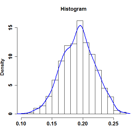
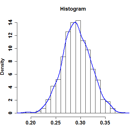
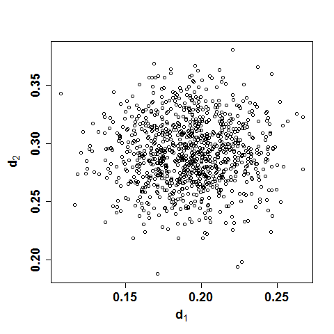
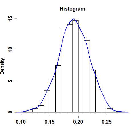
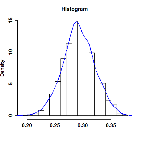
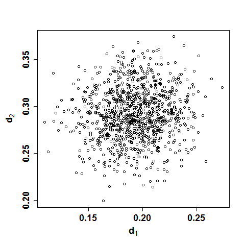
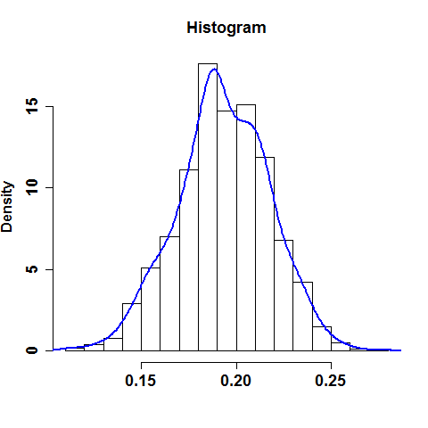
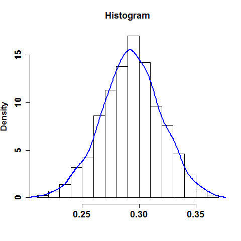
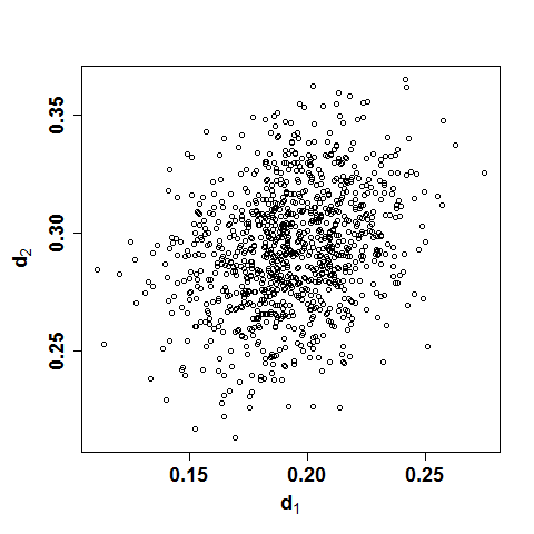
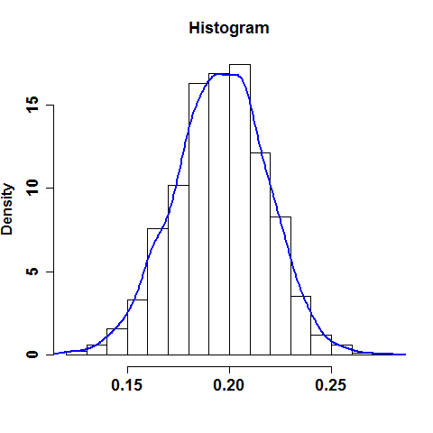
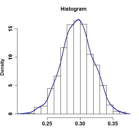
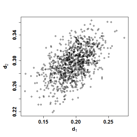
Figure 5.1: Histogram, kernel density and scatter plot of the SLOB estimated values of $\boldsymbol{d}_{0}=(0.2,0.3)$ for (a)–(c) $\rho=0$; (d)–(f) $\rho=0.3$; (g)–(i) $\rho=0.6$ and (j)–(l) $\rho=0.8$.

We also notice that the trade-off between bias and variance present in estimators of the spectral density function based on the smoothed periodogram does not seem to influence the estimation of the parameter $\boldsymbol{d}$. This is expected since the smoothed periodogram is a function of the observed time series alone which, by its turn, depends only on $\boldsymbol{d}_{0}$ and not on any particular estimated value $\widehat{\boldsymbol{d}}$, being, hence, a constant with respect to the latter.

Figure 5.1 depicts the behavior of the estimated values by presenting the histogram, kernel density estimates and the scatter plot of the SLOB estimated values for $(\alpha,\beta)=(0.85,0.9)$ and $\boldsymbol{d}=(0.2,0.3)$. Figures 5.1(a)–(c) correspond to $\rho=0$, Figures 5.1(d)–(f) to $\rho=0.3$, Figures 5.1(g)–(i) to $\rho=0.6$ and Figures 5.1(j)–(l) to $\rho=0.8$. Figure 5.1 reinforces the conjecture that the SLOB estimator is indeed asymptotically normally distributed.

6 Empirical Application

In this section we apply the LOB, SLOB and TLOB estimators considered in the last section to an exchange rate data set consisting of four daily exchange rates (business days) against the British Pound, namely, the US Dollar (USD/GBP), the Euro (EUR/GBP), the Japanese Yen (JPY/GBP) and the Swiss Franc (CHF/GBP). The data comprehend the period between October 2008 and July 2012, with sample size $n=1,684$. The data is similar to the one applied in Lobato (1999). The time series considered are the squared log-returns (squares of the first difference of the logarithm of the exchange rates) which is usually associated to the volatility of the returns (see, for instance, Cont, 2001). Our goal is to estimate the fractional differencing parameter $\boldsymbol{d}=(d_{1},d_{2},d_{3},d_{4})^{\prime}$, where the components are associated to the USD/GBP, the EUR/GBP, the JPY/GBP and the CHF/GBP exchange rates, respectively. In accordance to our findings in Section 5.3, for all estimators we apply $m=\lfloor n^{0.85}\rfloor=552$, while the cut-off point of the smoothed periodogram needed for the SLOB estimator is $\ell(n)=\lfloor n^{0.9}\rfloor=801$. For the SLOB estimator we apply the Bartlett’s weights and for the TLOB estimator, we apply the cosine-bell tapering function. For the SLOB estimator, we are assuming that it is indeed asymptotically normally distributed although, at this moment, we could not present a formal proof of the result, but we have empirical evidences that this is indeed true (see Table 5.1, Table 5.2 and Figure 5.1).

The correlation matrix of the data is presented on Table 6.1. As expected, all correlations are positive and high. Worth of note is the very high correlation between the squared returns of the USD/GBP and JPY/GBP exchange rates, over 0.85, which suggests a high association between the volatility on their exchange rates against the British Pound. Table 6.1 also presents the estimates of the fractional differencing parameter $\boldsymbol{d}$ obtained. In all cases the estimators pointed toward the existence of a mild long-range dependence on the data, characterized by the relatively small positive values of the estimated fractional differencing parameter. The estimated values obtained from the SLOB and TLOB estimators were all higher than the ones obtained from the LOB estimator.

Table 6.1: Estimated values of the fractional differencing parameter $\boldsymbol{d}$ and correlation matrix of the squared log-returns of the daily exchange rates data set for the LOB, SLOB and TLOB estimators.

Exchange rate	LOB	SLOB	TLOB	Correlation Matrix
				USD/GBP	EUR/GBP	JPY/GBP	CHF/GBP
USD/GBP	0.1065	0.1584	0.1546	1	0.4534	0.8552	0.4404
EUR/GBP	0.1459	0.1960	0.1895	0.4534	1	0.3273	0.4495
JPY/GBP	0.0596	0.1040	0.1030	0.8552	0.3273	1	0.4272
CHF/GBP	0.0960	0.1450	0.1421	0.4404	0.4495	0.4272	1

In both cases the estimated values point out for a greater persistence on the volatility of the EUR/GBP, USD/GBP, CHF/GBP and JPY/BPN exchange rates in this order. We observe that the estimated values of the fractional differencing parameter for the squared log-returns of the USD/GBP and the CHF/GBP exchange rates are remarkably close to one another. In order to apply the asymptotic results of Section 4, we shall test for the equality between them as well as the equality among the four fractional differencing parameters.

In order to do that, let $\widehat{\mathrm{G}}_{L}$, $\widehat{\mathrm{G}}_{S}$ and $\widehat{\mathrm{G}}_{T}$ denote the estimators of $G_{0}$ obtained by taking $f_{n}$ as the periodogram of the series, the smoothed periodogram with the Bartlett’s weights and the tapered periodogram with the cosine-bell tapering function, respectively. Also denote by $\widehat{\Omega}_{L}$, $\widehat{\Omega}_{S}$ and $\widehat{\Omega}_{T}$ the respective estimates of the matrix $\Omega$ as defined in Theorem 4.1 based on the pairs of estimates of $\widehat{\boldsymbol{d}}$ and $\widehat{G}$ obtained with the LOB, SLOB and TLOB estimators and the respective estimates of $G_{0}$. The estimates obtained are

$$\widehat{\Omega}_{L}=\left(\begin{array}[]{cccc}0.1410&0.0295&0.0776&0.0051\\ 0.0295&0.2002&0.0074&0.0133\\ 0.0776&0.0074&0.1502&0.0177\\ 0.0051&0.0133&0.0177&0.2146\\ \end{array}\right),\qquad\widehat{\Omega}_{S}=\left(\begin{array}[]{cccc}0.1438&0.0134&0.0867&0.0109\\ 0.0134&0.2131&0.0042&0.0198\\ 0.0867&0.0042&0.1505&0.0134\\ 0.0109&0.0198&0.0134&0.2068\\ \end{array}\right)$$

and

$$\widehat{\Omega}_{T}=\left(\begin{array}[]{cccc}0.2495&0.0003&0.0000&0.0002\\ 0.0003&0.2496&0.0001&0.0000\\ 0.0000&0.0001&0.2497&0.0002\\ 0.0002&0.0000&0.0002&0.2495\\ \end{array}\right).$$

Let us start by testing the equality of the fractional differencing parameters for the squared log-returns of the USD/GBP and the CHF/GBP exchange rates. In order words, we want to test the null hypothesis $H_{0}:d_{1}=d_{4}$. In this case, $R=(1,0,0,-1)$ and $\boldsymbol{\nu}=0$. The test statistics (4.5) under the null hypothesis is distributed according to a $\chi^{2}_{1}$ distribution. In this case, for the test statistics based on the LOB, SLOB and TLOB estimators, we have $T_{L}=0.1838$, $T_{S}=0.2986$ and $T_{T}=0.1745$ with all $p$-values $>0.58$. Therefore, we cannot reject the null hypothesis at any reasonable significance level and we conclude that the fractional differencing parameter of squared log-returns of the USD/GBP and CHF/GBP exchange rates are statistically equal. The question that naturally arises is are all fractional differencing parameters statistically equal? That is, we are interested in testing $H_{0}:d_{1}=\cdots=d_{4}$. In this case

$$R=\left(\begin{array}[]{cccc}1&-1&0&0\\ 0&1&-1&0\\ 0&0&1&-1\\ \end{array}\right)\qquad\mbox{and}\qquad\boldsymbol{\nu}=(0,0,0).$$

The values of the test statistics in this situation are $T_{L}=16.38$, $T_{S}=19.35$ and $T_{T}=8.45$, which, under the null hypothesis, are distributed according to a $\chi^{2}_{3}$ distribution. In this case, for the $T_{L}$ and $T_{S}$ test statistics, the $p$-values are both smaller than $0.001$ strongly indicating that the fractional differencing parameters of the series cannot be considered all equals at any reasonable significance level. The $T_{T}$ statistics also agrees (at 5% confidence level) with this conclusion, but with $p$-value equals to $0.038$.

7 Conclusions

In this work we propose and study a class of Gaussian semiparametric estimator of the fractional differencing parameter in multivariate long-range dependent processes. The main idea is to modify the approach of Shimotsu (2007) in order to introduce and analyze a generalization of the two-step estimator proposed by Lobato (1999) and studied in a slightly different form by Shimotsu (2007). More specifically, the idea is to consider the same objective function as in Lobato (1999), but considering an arbitrary spectral density matrix estimator in place of the periodogram. We consider two main cases: first, for an arbitrary consistent spectral density estimator, we show that the proposed estimator is also consistent. Secondly, we consider a class of spectral density estimator satisfying a single condition and show that the resulting estimator is consistent as well. The asymptotic distribution of the estimator under a certain condition on the spectral density estimator is derived and shown to be Gaussian with the same variance-covariance matrix as the one derived in Shimotsu (2007). Hypothesis testing are also discussed in connection with the asymptotic theory.

To assess the finite sample performance of the proposed estimator and to compare to the original one, we present a Monte Carlo simulation study based on VARFIMA$(0,\boldsymbol{d},0)$ processes. Under the conditions of the experiment, the proposed estimator shows an overall better performance over the original one. The approach is also applied to a financial data set consisting of daily exchange rates against the British Pound.

Acknowledgements

G. Pumi’s research was supported by a REUNI Pos-Doctoral fellowship from CAPES-Brazil via the REUNI program. S.R.C. Lopes’ research was partially supported by CNPq-Brazil, by Pronex Probabilidade e Processos Estocásticos - E-26/170.008/2008 -APQ1 and also by INCT em Matemática. The authors are grateful to the (Brazilian) National Center of Super Computing (CESUP-UFRGS) for the computational resources.

Appendix A: Proofs

In this section we present the proofs of the results in Sections 4 and 5. We establish lemmas and theorems in the same sequence as they appear in the text.

A.1 Proof of Theorem 3.1:

The proof follows the same lines as the proof of theorem 3(a) in Shimotsu (2007). First, without loss of generality let $0<\delta<1/2$ be fixed and consider the set $N_{\delta}\vcentcolon=\big{\{}\boldsymbol{d}:\|\boldsymbol{d}-\boldsymbol{d}_{0}\|_{\infty}>\delta\big{\}}$. Define $\boldsymbol{\theta}=(\theta_{1},\cdots,\theta_{q})^{\prime}\vcentcolon=\boldsymbol{d}-\boldsymbol{d}_{0}$ and let

$$L(\boldsymbol{d})\vcentcolon=S(\boldsymbol{d})-S(\boldsymbol{d}_{0}).$$

Let $0<\epsilon<1/4$ and define $\Theta_{1}\vcentcolon=\big{\{}\boldsymbol{\theta}:\boldsymbol{\theta}\in[-0.5+\epsilon,0.5]^{q}\big{\}}$ and $\Theta_{2}=\Omega_{\beta}\!\setminus\!\Theta_{1}$ (possibly an empty set), where $\Omega_{\beta}$ is given by (3.3). Following Robinson (1995b) and Shimotsu (2007), we have

$$\mathds{P}\big{(}\|\widehat{\boldsymbol{d}}-\boldsymbol{d}_{0}\|_{\infty}>\delta\big{)} \leq\mathds{P}\Big{(}\inf_{\overline{N_{\delta}}\cap\Omega_{\beta}}\!\!\big{\{}L(\boldsymbol{d})\big{\}}\leq 0\Big{)}$$

$$\leq\mathds{P}\Big{(}\inf_{\overline{N_{\delta}}\cap\Theta_{1}}\big{\{}L(\boldsymbol{d})\big{\}}\leq 0\Big{)}+\mathds{P}\Big{(}\inf_{\Theta_{2}}\big{\{}L(\boldsymbol{d})\big{\}}\leq 0\Big{)}\vcentcolon=P_{1}+P_{2},$$ (A.1)

where, for a given set $\mathcal{O}$, $\overline{\mathcal{O}}$ denotes the closure of $\mathcal{O}$. We shall show that $P_{1}$ and $P_{2}$ go to zero as $n$ tends to infinity. We deal with $P_{1}$ first. Notice that $L(\boldsymbol{d})$ can be rewritten as

$$L(\boldsymbol{d}) =\log\big{(}\det\{\widehat{G}(\boldsymbol{d})\}\big{)}-\log\big{(}\det\{\widehat{G}(\boldsymbol{d}_{0})\}\big{)}-2\sum_{k=1}^{q}\theta_{k}\frac{1}{m}\sum_{j=1}^{m}\log(\lambda_{j})$$

$$=\log\big{(}\det\{\widehat{G}(\boldsymbol{d})\}\big{)}-\log\big{(}\det\{\widehat{G}(\boldsymbol{d}_{0})\}\big{)}+\log\left(\frac{2\pi m}{n}\right)^{\!\!-2\sum_{k}\theta_{k}}-$$

$$\hskip 28.45274pt-2\sum_{k=1}^{q}\theta_{k}\bigg{(}\frac{1}{m}\sum_{j=1}^{m}\log(j)-\log(m)\bigg{)}-\sum_{k=1}^{q}\log(2\theta_{k}+1)$$

$$=\log\big{(}\mz{A}(\boldsymbol{d})\big{)}-\log\big{(}\mz{B}(\boldsymbol{d})\big{)}-\log\big{(}\mz{A}(\boldsymbol{d}_{0})\big{)}+\log\big{(}\mz{B}(\boldsymbol{d}_{0})\big{)}+\mz{R}(\boldsymbol{d})$$

$$=Q_{1}(\boldsymbol{d})-Q_{2}(\boldsymbol{d})+\mz{R}(\boldsymbol{d}),$$ (A.2)

where

$$Q_{1}(\boldsymbol{d})\vcentcolon=\log\big{(}\mz{A}(\boldsymbol{d})\big{)}-\log\big{(}\mz{B}(\boldsymbol{d})\big{)},\qquad Q_{2}(\boldsymbol{d})\vcentcolon=\log\big{(}\mz{A}(\boldsymbol{d}_{0})\big{)}+\log\big{(}\mz{B}(\boldsymbol{d}_{0})\big{)},$$

$$\mz{A}(\boldsymbol{d})\vcentcolon=\left(\frac{2\pi m}{n}\right)^{\!\!-2\sum_{k}\theta_{k}}\!\!\det\{\widehat{G}(\boldsymbol{d})\},\qquad\mz{B}(\boldsymbol{d})\vcentcolon=\det\{G_{0}\}\prod_{k=1}^{q}\frac{1}{2\theta_{k}+1},$$

$$\mbox{ and }\quad\mz{R}(\boldsymbol{d})\vcentcolon=2\sum_{k=1}^{q}\theta_{k}\bigg{(}\log(m)-\frac{1}{m}\sum_{j=1}^{m}\log(j)\bigg{)}-\sum_{k=1}^{q}\log(2\theta_{k}+1).\phantom{andanda}$$

By lemma 2 in Robinson (1995b), $\log(m)-m^{-1}\sum_{j=1}^{m}\log(j)=1+O(m^{-1}\log(m))$, so that

$$\mz{R}(\boldsymbol{d})=\sum_{k=1}^{q}\Big{[}2\theta_{k}-\log(2\theta_{k}+1)\Big{]}+O\left(\frac{\log(m)}{m}\right).$$

Since $x-\log(x+1)$ has a unique global minimum in $(-1,\infty)$ at $x=0$ and $x-\log(x+1)\geq x^{2}/4$, for $|x|\leq 1$, it follows that

$$\inf_{\overline{N_{\delta}}\cap\Theta_{1}}\!\!\big{\{}\mz{R}(\boldsymbol{d})\big{\}}\geq\frac{1}{4}\Big{(}2\max_{k}\{\theta_{k}\}\Big{)}^{2}\geq\delta^{2}>0\,.$$ (A.3)

In view of (A.1) and (A.3), in order to show that $P_{1}\rightarrow 0$ it suffices to show the existence of a function $h(\boldsymbol{d})>0$ satisfying

$$(\mathrm{i})\,\,\sup_{\Theta_{1}}\big{\{}\big{|}\mz{A}(\boldsymbol{d})-h(\boldsymbol{d})\big{|}\big{\}}=o_{\mathds{P}}(1);\quad(\mathrm{ii})\,\,h(\boldsymbol{d})\geq\mz{B}(\boldsymbol{d});\quad(\mathrm{iii})\,\,h(\boldsymbol{d}_{0})=\mz{B}(\boldsymbol{d}_{0}),$$ (A.4)

as $n$ goes to infinity, because (ii) implies $\displaystyle{\inf_{\Theta_{1}}}\big{\{}h(\boldsymbol{d})\big{\}}\geq\displaystyle{\inf_{\Theta_{1}}}\big{\{}\mz{B}(\boldsymbol{d})\big{\}}>0$, so that,

$$Q_{1}(\boldsymbol{d})\geq\log\big{(}\mz{A}(\boldsymbol{d})\big{)}-\log\big{(}h(\boldsymbol{d})\big{)}=\log\big{(}h(\boldsymbol{d})+o_{\mathds{P}}(1)\big{)}-\log\big{(}h(\boldsymbol{d})\big{)}=o_{\mathds{P}}(1),$$

and (iii) implies $Q_{2}(\boldsymbol{d})=\log\big{(}h(\boldsymbol{d}_{0})+o_{\mathds{P}}(1)\big{)}-\log\big{(}h(\boldsymbol{d}_{0})\big{)}=o_{\mathds{P}}(1)$, both asymptotic orders being uniform in $\Theta_{1}$ in view of (i), and these results together with (A.3) imply $P_{1}\!\!\longrightarrow\!0$.

To show (i), recall that

$$\Lambda_{j}(\boldsymbol{d})^{-1} =\!\!\operatorname*{\mathrm{diag}}_{k\in\{1,\cdots,q\}}\!\!\{\lambda_{j}^{d_{k}}\mathrm{e}^{\mathrm{i}(\lambda_{j}-\pi)d_{k}/2}\}=\!\!\operatorname*{\mathrm{diag}}_{k\in\{1,\cdots,q\}}\!\!\{\lambda_{j}^{(d_{k}-d_{k}^{0})}\mathrm{e}^{\mathrm{i}(\lambda_{j}-\pi)(d_{k}-d_{k}^{0})/2}\!\times\!\lambda_{j}^{d_{k}^{0}}\mathrm{e}^{\mathrm{i}(\lambda_{j}-\pi)d_{k}^{0}/2}\}$$

$$=\Lambda_{j}(\boldsymbol{d}-\boldsymbol{d}_{0})^{-1}\Lambda_{j}(\boldsymbol{d}_{0})^{-1}=\Lambda_{j}(\boldsymbol{\theta})^{-1}\Lambda_{j}(\boldsymbol{d}_{0})^{-1}\!,$$ (A.5)

so that we can write

$$\mz A (\boldsymbol{d})=\left(\frac{2\pi m}{n}\right)^{\!\!-2\sum_{k}\theta_{k}}\!\!\times\det\bigg{\{}\frac{1}{m}\sum_{j=1}^{m}\mathrm{Re}\big{[}\Lambda_{j}(\boldsymbol{\theta})^{-1}\Lambda_{j}(\boldsymbol{d}_{0})^{-1}f_{n}(\lambda_{j})\overline{\Lambda_{j}(\boldsymbol{d}_{0})^{-1}}^{\,\,\prime}\overline{\Lambda_{j}(\boldsymbol{\theta})^{-1}}^{\,\,\prime}\big{]}\bigg{\}}$$

$$=\det\bigg{\{}\frac{1}{m}\sum_{j=1}^{m}\mathrm{Re}\big{[}M_{j}(\boldsymbol{\theta})\Lambda_{j}(\boldsymbol{d}_{0})^{-1}\big{(}f(\lambda_{j})+o_{\mathds{P}}(n^{-\beta})\big{)}\overline{\Lambda_{j}(\boldsymbol{d}_{0})^{-1}}^{\,\,\prime}\overline{M_{j}(\boldsymbol{\theta})}^{\,\,\prime}\big{]}\bigg{\}}$$

$$=\det\bigg{\{}\frac{1}{m}\sum_{j=1}^{m}\mathrm{Re}\big{[}M_{j}(\boldsymbol{\theta})G_{0}\overline{M_{j}(\boldsymbol{\theta})}^{\,\,\prime}\big{]}+\frac{1}{m}\sum_{j=1}^{m}\mathrm{Re}\big{[}M_{j}(\boldsymbol{\theta})\Lambda_{j}(\boldsymbol{d}_{0})^{-1}o_{\mathds{P}}(n^{-\beta})\overline{\Lambda_{j}(\boldsymbol{d}_{0})^{-1}}^{\,\,\prime}\overline{M_{j}(\boldsymbol{\theta})}^{\,\,\prime}\big{]}\bigg{\}},$$ (A.6)

where $M_{j}(\boldsymbol{\theta}):=\operatorname*{\mathrm{diag}}_{k\in\{1,\cdots,q\}}\Big{\{}\mathrm{e}^{\mathrm{i}(\lambda_{j}-\pi){d}_{k}^{0}/2}(j/m)^{\theta_{k}}\Big{\}}$. By omitting the $\mathrm{Re}[\cdot]$ operator, the $(r,r)$-th element in the second term inside the determinant on the right-hand side of (A.1) is

$$\frac{1}{m}\sum_{j=1}^{m}\bigg{(}\frac{j}{m}\bigg{)}^{2\theta_{r}}\lambda_{j}^{2d_{r}^{0}}o_{\mathds{P}}(n^{-\beta})=o_{\mathds{P}}(1)\frac{1}{m}\sum_{j=1}^{m}\bigg{(}\frac{j}{m}\bigg{)}^{2\theta_{r}}j^{2d_{r}^{0}}=o_{\mathds{P}}(1)\frac{1}{m^{2d_{r}^{0}+1}}\sum_{j=1}^{m}\bigg{(}\frac{j}{m}\bigg{)}^{2d_{r}},$$ (A.7)

since $\boldsymbol{d}_{0}\in\Omega_{\beta}$. Now, by taking $\gamma=2d_{r}+1>0$ in lemma 1 in Robinson (1995b), it follows that

$$\frac{1}{m}\sum_{j=1}^{m}\bigg{(}\frac{j}{m}\bigg{)}^{2d_{r}} =\frac{1}{2d_{r}+1}\bigg{[}\frac{2d_{r}+1}{m}\sum_{j=1}^{m}\bigg{(}\frac{j}{m}\bigg{)}^{2d_{r}}\bigg{]}=\frac{1}{2d_{r}+1}\big{[}O(m^{\beta-1})+1\big{]}$$ (A.8)

so that (A.7) is $o_{\mathds{P}}(1)$ uniformly in $\Theta_{1}$ in view of (A.8) and since $\boldsymbol{d}_{0}\in\Omega_{\beta}$ by hypothesis and $\boldsymbol{d}\in\Omega_{\beta}$ by the definition of the estimator. Hence, the second term inside the determinant on the right-hand side of (A.1) is $o_{\mathds{P}}(1)$ uniformly in $\Theta_{1}$, so that

$$\mz A (\boldsymbol{d})=\det\bigg{\{}\frac{1}{m}\sum_{j=1}^{m}\mathrm{Re}\big{[}M_{j}(\boldsymbol{\theta})G_{0}\overline{M_{j}(\boldsymbol{\theta})}^{\,\,\prime}\big{]}+o_{\mathds{P}}(1)\bigg{\}}.$$ (A.9)

Upon defining the matrices

$$\mathcal{E}_{0}:=\operatorname*{\mathrm{diag}}_{k\in\{1,\cdots,q\}}\Big{\{}\mathrm{e}^{\mathrm{i}\pi d_{k}^{0}/2}\Big{\}},\quad\mathcal{G}_{0}:=\mathrm{Re}\big{[}\mathcal{E}_{0}G_{0}\overline{\mathcal{E}_{0}}^{\,\,\prime}\big{]}\ \ \mbox{ and }\ \ \mathcal{M}(\boldsymbol{\theta}):=\left(\frac{1}{1+\theta_{r}+\theta_{s}}\right)_{r,s=1}^{q}$$

from the proof of theorem 3(a) in Shimotsu (2007), it follows that the function

$$h(\boldsymbol{d}):=\det\Big{\{}\mathcal{M}(\boldsymbol{\theta})\odot\mathcal{G}_{0}\Big{\}},$$

where $\odot$ denotes the Hadamard product, satisfies the conditions (i), (ii) and (iii) in (A.4) (notice that (A.9) is the same equation as the one following (40) in Shimotsu, 2007, p.303, with the obvious identifications).

Now we move to bound $P_{2}$. By using (A.1), rewrite $L(\boldsymbol{d})$ as

$$L(\boldsymbol{d})=\log\Big{(}\det\big{\{}\widehat{\mathcal{D}}(\boldsymbol{d})\big{\}}\Big{)}-\log\Big{(}\det\big{\{}\widehat{\mathcal{D}}(\boldsymbol{d}_{0})\big{\}}\Big{)},$$ (A.10)

where

$$\widehat{\mathcal{D}}(\boldsymbol{d})\vcentcolon=\frac{1}{m}\sum_{j=1}^{m}\mathrm{Re}\big{[}\mathcal{P}_{j}(\boldsymbol{\theta})\Lambda_{j}(\boldsymbol{d}_{0})^{-1}f_{n}(\lambda_{j})\overline{\Lambda_{j}(\boldsymbol{d}_{0})^{-1}}^{\,\,\prime}\overline{\mathcal{P}_{j}(\boldsymbol{\theta})}^{\,\,\prime}\big{]},$$

with

$$\mathcal{P}_{j}(\boldsymbol{\theta})\vcentcolon=\operatorname*{\mathrm{diag}}_{k\in\{1,\cdots,q\}}\bigg{\{}\mathrm{e}^{\mathrm{i}(\lambda_{j}-\pi)d^{0}_{k}/2}\left(\frac{j}{\mz p}\right)^{\!\!\theta_{k}}\bigg{\}}\quad\mbox{and}\quad\mz p\vcentcolon=\exp\bigg{(}\frac{1}{m}\sum_{j=1}^{m}\log(j)\bigg{)},$$

and, as $m$ tends to infinity, $\mz p\sim m/\mathrm{e}$. Observe that $\widehat{\mathcal{D}}(\boldsymbol{d})$ is positive semidefinite since each summand of $\widehat{\mathcal{D}}$ is. For $\kappa\in(0,1)$, define the auxiliary functions

$$\widehat{\mathcal{D}}_{\kappa}(\boldsymbol{d})\vcentcolon=\frac{1}{m}\sum_{j=\lfloor m\kappa\rfloor}^{m}\!\mathrm{Re}\big{[}\mathcal{P}_{j}(\boldsymbol{\theta})\Lambda_{j}(\boldsymbol{d}_{0})^{-1}f_{n}(\lambda_{j})\overline{\Lambda_{j}(\boldsymbol{d}_{0})^{-1}}^{\,\,\prime}\overline{\mathcal{P}_{j}(\boldsymbol{\theta})}^{\,\,\prime}\big{]}$$

and

$$\mathcal{Q}_{\kappa}(\boldsymbol{d})\vcentcolon=\frac{1}{m}\sum_{j=\lfloor m\kappa\rfloor}^{m}\!\mathrm{Re}\big{[}\mathcal{P}_{j}(\boldsymbol{\theta})G_{0}\overline{\mathcal{P}_{j}(\boldsymbol{\theta})}^{\,\,\prime}\big{]},$$

where $\lfloor x\rfloor$ denotes the integer part of $x$. Now, by the hypothesis on $f_{n}$,

$$\widehat{\mathcal{D}}_{\kappa}(\boldsymbol{d}) =\frac{1}{m}\sum_{j=\lfloor m\kappa\rfloor}^{m}\!\mathrm{Re}\big{[}\mathcal{P}_{j}(\boldsymbol{\theta})\Lambda_{j}(\boldsymbol{d}_{0})^{-1}\big{(}f(\lambda_{j})+o_{\mathds{P}}(n^{-\beta})\big{)}\overline{\Lambda_{j}(\boldsymbol{d}_{0})^{-1}}^{\,\,\prime}\overline{\mathcal{P}_{j}(\boldsymbol{\theta})}^{\,\,\prime}\big{]}$$

$$=\mathcal{Q}_{\kappa}(\boldsymbol{d})+o(1)+\frac{1}{m}\sum_{j=\lfloor m\kappa\rfloor}^{m}\mathrm{Re}\big{[}\mathcal{P}_{j}(\boldsymbol{\theta})\Lambda_{j}(\boldsymbol{d}_{0})^{-1}o_{\mathds{P}}(n^{-\beta})\overline{\Lambda_{j}(\boldsymbol{d}_{0})^{-1}}^{\,\,\prime}\overline{\mathcal{P}_{j}(\boldsymbol{\theta})}^{\,\,\prime}\big{]},$$ (A.11)

where the last equality follows from lemma 5.4 in Shimotsu and Phillips (2005). The $(r,s)$-th element of the third term on the RHS of (A.1) is given by

$$\mathrm{Re}\bigg{[}\frac{1}{m}\sum_{j=\lfloor m\kappa\rfloor}^{m}\left(\frac{j}{\mz p}\right)^{\!\!\theta_{r}+\theta_{s}} \left(\frac{2\pi j}{n}\right)^{\!\!d^{0}_{r}+d^{0}_{s}}\mathrm{e}^{\mathrm{i}(\lambda_{j}-\pi)(\theta_{r}-\theta_{s})/2}o_{\mathds{P}}(n^{-\beta})\bigg{]}=$$

$$=O(1)\left(\frac{m}{\mz p}\right)^{\!\!\theta_{r}+\theta_{s}}\left(\frac{m}{n}\right)^{\!\!d^{0}_{r}+d^{0}_{s}}o_{\mathds{P}}(n^{-\beta})\,\frac{1}{m}\sum_{j=\lfloor m\kappa\rfloor}^{m}\left(\frac{j}{m}\right)^{\!\!2(d^{0}_{r}+d^{0}_{s})-(\widehat{d}_{r}+\widehat{d}_{s})}$$

$$=O(1)o_{\mathds{P}}(1)\left(\frac{m}{\mz p}\right)^{\!\!\theta_{r}+\theta_{s}}O(1)=o_{\mathds{P}}(1),$$

uniformly in $\boldsymbol{\theta}\in\Theta_{2}$, since $\boldsymbol{d}_{0}\in\Omega_{\beta}$, $\beta\in(0,1)$ and Assumption A4, where the penultimate equality follows from lemma 5.4 in Shimotsu and Phillips (2005). This shows that

$$\sup_{\Theta_{2}}\big{\{}\big{|}\det\{\widehat{\mathcal{D}}(\boldsymbol{d})\}-\det\{\mathcal{Q}_{\kappa}(\boldsymbol{d})\}\big{|}\big{\}}=o_{\mathds{P}}(1).$$

The proof now follows viz a viz (with the obvious notational identification) from the proof of theorem 3(a) in Shimotsu (2007), p.303 (see the argument following equation (42)). From this, we conclude that $P_{2}\longrightarrow 0$, as $n$ tends to infinity, and this completes the proof. $\blacksquare$

A.2 Proof of Lemma 3.1

For fixed $r,s\in\{1,\cdots,q\}$, let $\mathscr{A}_{uv}\vcentcolon=\sum_{j=u}^{v}\mathscr{A}_{j}$ and $\mathscr{B}_{uv}\vcentcolon=\sum_{j=u}^{v}\mathscr{B}_{j}$, where

$$\mathscr{A}_{j}\vcentcolon=\mathrm{e}^{\mathrm{i}(\lambda_{j}-\pi)(d_{r}^{0}-d_{s}^{0})/2}\lambda_{j}^{d^{0}_{r}+d^{0}_{s}}\big{[}f_{n}^{rs}(\lambda_{j})-\big{(}A(\lambda_{j})\big{)}_{r\boldsymbol{\cdot}}I_{\boldsymbol{\varepsilon}}(\lambda_{j})\big{(}\overline{A(\lambda_{j})}^{\,\,\prime}\big{)}_{\boldsymbol{\cdot}s}\big{]},$$ (A.12)

and

$$\mathscr{B}_{j}\vcentcolon=\mathrm{e}^{\mathrm{i}(\lambda_{j}-\pi)(d_{r}^{0}-d_{s}^{0})/2}\lambda_{j}^{d^{0}_{r}+d^{0}_{s}}\big{(}A(\lambda_{j})\big{)}_{r\boldsymbol{\cdot}}I_{\boldsymbol{\varepsilon}}(\lambda_{j})\big{(}\overline{A(\lambda_{j})}^{\,\,\prime}\big{)}_{\boldsymbol{\cdot}s}-G_{0}^{rs}.$$ (A.13)

Hence, for each $j$, $\mathscr{A}_{j}+\mathscr{B}_{j}=\mathrm{e}^{\mathrm{i}(\lambda_{j}-\pi)(d_{r}^{0}-d_{s}^{0})/2}\lambda_{j}^{d^{0}_{r}+d^{0}_{s}}f_{n}^{rs}(\lambda_{j})-G_{0}^{rs}$. For fixed $u\leq j\leq v$, we have

$$\mathds{E}\big{(}|\mathscr{A}_{j}|\big{)} =(2\pi)^{d_{r}^{0}+d_{s}^{0}}\mathds{E}\Big{(}\lambda_{j}^{-d^{0}_{r}-d^{0}_{s}}\Big{|}f_{n}^{rs}(\lambda_{j})-\big{(}A(\lambda_{j})\big{)}_{r\boldsymbol{\cdot}}I_{\boldsymbol{\varepsilon}}(\lambda_{j})\big{(}\overline{A(\lambda_{j})}^{\,\,\prime}\big{)}_{\boldsymbol{\cdot}s}\Big{|}\Big{)}\ =\ o(1)$$

$$=(2\pi)^{d_{r}^{0}+d_{s}^{0}}o(1)\,\,=\,\,o(1),$$

from where we conclude that $\displaystyle{\max_{r,s}}$ $\!\big{\{}\mathds{E}\big{(}\big{|}\sum_{j=u}^{v}\mathscr{A}_{j}\big{|}\big{)}\big{\}}=o(v-u+1)$ and the result on $\mathscr{A}_{uv}$ follows. As for $\mathscr{B}_{j}$, from the proof of lemma 1(a) in Shimotsu (2007) (notice that $\mathscr{B}_{j}$ does not depend on $f_{n}$) it follows that $\sum_{j=u}^{v}\mathscr{B}_{j}=o_{\mathds{P}}(v)$ uniformly in $u$ and $v$ and hence the desired result on $\mathscr{B}_{uv}$ follows. The last assertion is now straightforward. $\blacksquare$

A.3 Proof of Theorem 3.2

By carefully inspecting the proof of Theorem 3.1, we observe that it suffices to show (with the same notation as in the aforementioned proof) (A.9) uniformly in $\Theta_{1}$ and that $\widehat{\mathcal{D}}_{\kappa}(\boldsymbol{d})-\mathcal{Q}_{\kappa}(\boldsymbol{d})=o_{\mathds{P}}(1)$ uniformly in $\Theta_{2}$. To show (A.9), it suffices to show that

$$\frac{1}{m}\sum_{j=1}^{m}\mathrm{Re}\Big{[}M_{j}(\boldsymbol{\theta})\Lambda_{j}(\boldsymbol{d}_{0})^{-1}f_{n}(\lambda_{j})\overline{\Lambda_{j}(\boldsymbol{d}_{0})^{-1}}^{\,\,\prime}\overline{M_{j}(\boldsymbol{\theta})}^{\,\,\prime}\Big{]}=\frac{1}{m}\sum_{j=1}^{m}\mathrm{Re}\Big{[}M_{j}(\boldsymbol{\theta})G_{0}\overline{M_{j}(\boldsymbol{\theta})}^{\,\,\prime}\Big{]}+o_{\mathds{P}}(1).$$ (A.14)

The $(r,s)$-th component of the LHS of (A.14) is given by

$$\frac{1}{m}\sum_{j=1}^{m}\mathrm{Re}\bigg{[}\mathrm{e}^{\mathrm{i}(\lambda_{j}-\pi)(d^{0}_{r}-d^{0}_{s})/2}\left(\frac{j}{m}\right)^{\theta_{r}+\theta_{s}}\!\!f_{n}^{rs}(\lambda_{j})\Big{(}\Lambda_{j}^{(r)}(\boldsymbol{d}_{0})\overline{\Lambda_{j}^{(s)}(\boldsymbol{d}_{0})}^{\,\,\prime}\Big{)}^{-1}\bigg{]}.$$

Summation by parts (see Zygmund, 2002, p.3) yields

$$\sup_{\Theta_{1}}\bigg{\{}\bigg{|}\frac{1}{m} \sum_{j=1}^{m}\mathrm{e}^{\mathrm{i}(\lambda_{j}-\pi)(d^{0}_{r}-d^{0}_{s})/2}\left(\frac{j}{m}\right)^{\theta_{r}+\theta_{s}}\!\!\Big{[}f_{n}^{rs}(\lambda_{j})\Big{(}\Lambda_{j}^{(r)}(\boldsymbol{d}_{0})\overline{\Lambda_{j}^{(s)}(\boldsymbol{d}_{0})}^{\,\,\prime}\Big{)}^{\!\!-1}\!\!\!-G_{0}^{rs}\Big{]}\bigg{|}\bigg{\}}\leq$$

$$\leq\frac{1}{m}\sum_{k=1}^{m-1}\sup_{\Theta_{1}}\bigg{\{}\bigg{|}\mathrm{e}^{\mathrm{i}(\lambda_{k}-\pi)(d^{0}_{r}-d^{0}_{s})/2}\left(\frac{k}{m}\right)^{\theta_{r}+\theta_{s}}-\mathrm{e}^{\mathrm{i}(\lambda_{k+1}-\pi)(d^{0}_{r}-d^{0}_{s})/2}\left(\frac{k+1}{m}\right)^{\theta_{r}+\theta_{s}}\bigg{|}\bigg{\}}\times$$

$$\hskip 56.9055pt\times\,\,\,\bigg{|}\sum_{j=1}^{k}\Big{[}f_{n}^{rs}(\lambda_{j})\Big{(}\Lambda_{j}^{(r)}(\boldsymbol{d}_{0})\overline{\Lambda_{j}^{(s)}(\boldsymbol{d}_{0})}^{\,\,\prime}\Big{)}^{\!\!-1}\!\!\!-G_{0}^{rs}\Big{]}\bigg{|}\ +$$

$$\hskip 85.35826pt+\,\,\,\bigg{|}\frac{1}{m}\sum_{j=1}^{m}\Big{[}f_{n}^{rs}(\lambda_{j})\Big{(}\Lambda_{j}^{(r)}(\boldsymbol{d}_{0})\overline{\Lambda_{j}^{(s)}(\boldsymbol{d}_{0})}^{\,\,\prime}\Big{)}^{\!\!-1}\!\!\!-G_{0}^{rs}\Big{]}\bigg{|}$$

$$\leq\mz C\sum_{k=1}^{m-1}\left(\frac{k}{m}\right)^{\!\!2\epsilon}\frac{1}{k^{2}}\bigg{|}\sum_{j=1}^{k}\Big{[}f_{n}^{rs}(\lambda_{j})\Big{(}\Lambda_{j}^{(r)}(\boldsymbol{d}_{0})\overline{\Lambda_{j}^{(s)}(\boldsymbol{d}_{0})}^{\,\,\prime}\Big{)}^{\!\!-1}\!\!\!-G_{0}^{rs}\Big{]}\bigg{|}\ +$$

$$\hskip 56.9055pt+\,\,\,\bigg{|}\frac{1}{m}\sum_{j=1}^{m}\Big{[}f_{n}^{rs}(\lambda_{j})\Big{(}\Lambda_{j}^{(r)}(\boldsymbol{d}_{0})\overline{\Lambda_{j}^{(s)}(\boldsymbol{d}_{0})}^{\,\,\prime}\Big{)}^{\!\!-1}\!\!\!-G_{0}^{rs}\Big{]}\bigg{|},$$ (A.15)

where $0<\mz C<\infty$ is a constant. The first term in (A.3) is, by (3.5),

$$\sum_{k=1}^{m-1}\left(\frac{k}{m}\right)^{2\epsilon}\!\!\!\frac{1}{k^{2}}\bigg{|}\sum_{j=1}^{k}\Big{[}f_{n}^{rs}(\lambda_{j}) \Big{(}\Lambda_{j}^{(r)}(\boldsymbol{d}_{0})\overline{\Lambda_{j}^{(s)}(\boldsymbol{d}_{0})}^{\,\,\prime}\Big{)}^{\!\!-1}\!\!\!-G_{0}^{rs}\Big{]}\bigg{|}\leq\sum_{k=1}^{m-1}\left(\frac{k}{m}\right)^{2\epsilon}\!\!\!\frac{1}{k^{2}}\Big{(}\big{|}\mathscr{A}_{1k}\big{|}+\big{|}\mathscr{B}_{1k}\big{|}\Big{)}$$

$$=\frac{1}{m^{2\epsilon}}\sum_{k=1}^{m-1}k^{2(\epsilon-1)}\big{|}\mathscr{A}_{1k}\big{|}+\frac{1}{m^{2\epsilon}}\sum_{k=1}^{m-1}k^{2(\epsilon-1)}o_{\mathds{P}}(k)=o_{\mathds{P}}(1),$$ (A.16)

uniformly in $(r,s)$, where the last equality follows from lemma 2 in Robinson (1995b), Lemma 3.1 and Chebyshev’s inequality, since

$$\mathds{E}\left(\frac{1}{m^{2\epsilon}}\sum_{k=1}^{m-1}k^{2(\epsilon-1)}\big{|}\mathscr{A}_{1k}\big{|}\right) =\frac{2\epsilon}{m}\,\sum_{k=1}^{m-1}{\left(\frac{k}{m}\right)}^{2\epsilon-1}\frac{1}{k}\,\mathds{E}\Big{(}\big{|}\mathscr{A}_{1k}\big{|}\Big{)}=\big{[}1+O(m^{-\epsilon})\big{]}o(1)=o(1).$$

The second term in (A.3) is $o_{\mathds{P}}(1)$ uniformly in $(r,s)$ by (3.5). Hence, (A.14) follows. As for the difference $\widehat{\mathcal{D}}_{\kappa}(\boldsymbol{d})-\mathcal{Q}_{\kappa}(\boldsymbol{d})$, its $(r,s)$-th element is given by

$$\frac{1}{m}\sum_{j=\lfloor m\kappa\rfloor}^{m}\! \mathrm{Re}\bigg{[}\mathrm{e}^{\mathrm{i}(\lambda_{j}-\pi)(d^{0}_{r}-d^{0}_{s})/2}\left(\frac{j}{\mz p}\right)^{\theta_{r}+\theta_{s}}\!\!\Big{[}f_{n}^{rs}(\lambda_{j})\Big{(}\Lambda_{j}^{(r)}(\boldsymbol{d}_{0})\overline{\Lambda_{j}^{(s)}(\boldsymbol{d}_{0})}^{\,\,\prime}\Big{)}^{\!\!-1}\!\!\!-G_{0}^{rs}\Big{]}\bigg{]}=$$

$$=\left(\frac{m}{\mz p}\right)^{d^{0}_{r}+d^{0}_{s}}\!\!\mathrm{Re}\bigg{[}\frac{1}{m}\sum_{j=\lfloor m\kappa\rfloor}^{m}\mathrm{e}^{\mathrm{i}(\lambda_{j}-\pi)(\theta_{r}-\theta_{s})/2}\left(\frac{j}{m}\right)^{\theta_{r}+\theta_{s}}\!\!\!\times\Big{[}f_{n}^{rs}(\lambda_{j})\Big{(}\Lambda_{j}^{(r)}(\boldsymbol{d}_{0})\overline{\Lambda_{j}^{(s)}(\boldsymbol{d}_{0})}^{\,\,\prime}\Big{)}^{\!\!-1}\!\!\!-G_{0}^{rs}\Big{]}\bigg{]}$$

which is $o_{\mathds{P}}(1)$ uniformly in $\boldsymbol{\theta}\in\Theta_{2}$ by similar argument as the one applied in deriving (A.3), from summation by parts and lemma 5.4 in Shimotsu and Phillips (2005). This completes the proof. $\blacksquare$

A.4 Proof of Lemma 4.1

(a) For $r,s\in\{1,\cdots,q\}$ fixed, ignoring the maximum in expression (4.2) for a while, we see that if $d_{r}^{0}+d_{s}^{0}\geq 0$,

$$\sum_{j=1}^{v}\lambda_{j}^{d_{r}^{0}+d_{s}^{0}} \Big{[}f_{n}^{rs}(\lambda_{j})-\big{(}A(\lambda_{j})\big{)}_{r\boldsymbol{\cdot}}I_{\boldsymbol{\varepsilon}}(\lambda_{j})\big{(}\overline{A(\lambda_{j})}^{\,\,\prime}\big{)}_{\boldsymbol{\cdot}s}\Big{]}\leq$$

$$\leq\ \max\big{\{}1,n^{|d_{r}^{0}+d_{s}^{0}|}\big{\}}\max_{1\leq v\leq m}\bigg{\{}\sum_{j=1}^{v}\Big{[}f_{n}^{rs}(\lambda_{j})-\big{(}A(\lambda_{j})\big{)}_{r\boldsymbol{\cdot}}I_{\boldsymbol{\varepsilon}}(\lambda_{j})\big{(}\overline{A(\lambda_{j})}^{\,\,\prime}\big{)}_{\boldsymbol{\cdot}s}\Big{]}\bigg{\}}$$

$$=\ o_{\mathds{P}}\left(\frac{m^{2}}{n}\right)\ =\ o_{\mathds{P}}\left(\frac{\sqrt{m}}{\log(m)}\right),$$

where the last equality follows since Assumption B4 holds for $\alpha=1$, which implies $mn^{-1}=o\big{(}m^{-1/2}\log(m)^{-1}\big{)}$.

(b) Rewrite the argument of the summation in (4.3) as $\mathscr{A}_{j}+\mathscr{B}_{j}+\mathscr{C}_{j}$, where

$$\mathscr{A}_{j} :=\lambda_{j}^{d_{r}^{0}+d_{s}^{0}}\Big{[}f_{n}^{rs}(\lambda_{j})-\big{(}A(\lambda_{j})\big{)}_{r\boldsymbol{\cdot}}I_{\boldsymbol{\varepsilon}}(\lambda_{j})\big{(}\overline{A(\lambda_{j})}^{\,\,\prime}\big{)}_{\boldsymbol{\cdot}s}\Big{]},$$

$$\mathscr{B}_{j} :=\lambda_{j}^{d_{r}^{0}+d_{s}^{0}}\Big{[}\big{(}A(\lambda_{j})\big{)}_{r\boldsymbol{\cdot}}I_{\boldsymbol{\varepsilon}}(\lambda_{j})\big{(}\overline{A(\lambda_{j})}^{\,\,\prime}\big{)}_{\boldsymbol{\cdot}s}-f_{rs}(\lambda_{j})\Big{]},$$

$$\mathscr{C}_{j} :=\lambda_{j}^{d_{r}^{0}+d_{s}^{0}}f_{rs}(\lambda_{j})-\mathrm{e}^{\mathrm{i}(\pi-\lambda_{j})(d_{r}^{0}-d_{s}^{0})/2}G_{0}^{rs}.$$

Part (a) yields $\max_{v}\Big{\{}\max_{r,s}\Big{\{}\!\!\sum_{j=1}^{v}\big{|}\mathscr{A}_{j}\big{|}\Big{\}}\Big{\}}=o_{\mathds{P}}\Big{(}m^{1/2}\big{(}\log(m)\big{)}^{-1}\Big{)}$, while, from the proof of lemma 1(b2) in Shimotsu (2007), we obtain $\max_{r,s}\Big{\{}\!\!\sum_{j=1}^{v}\big{|}\mathscr{B}_{j}\big{|}\Big{\}}=O_{\mathds{P}}\big{(}v^{1/2}\log(v)\big{)}$ (recall that $\mathrm{e}^{\mathrm{i}\lambda_{j}}=O(\lambda_{j})$). Assumption B1 implies that $|\mathscr{C}_{j}|=O(\lambda_{j}^{\alpha})$ regardless $r,s$ so that $\max_{r,s}\Big{\{}\!\!\sum_{j=1}^{v}\big{|}\mathscr{C}_{j}\big{|}\Big{\}}=O\big{(}v^{\alpha+1}n^{-\alpha}\big{)}$. The result now follows by noticing that $m^{1/2}\big{(}\log(m)\big{)}^{-1}=O\big{(}m^{1/2}\log(m)\big{)}$. $\blacksquare$

A.5 Proof of Theorem 4.1

The argument is similar to the one in the proof of theorem 3(b) in Shimotsu (2007). By hypothesis, with probability tending to 1 as $n$ tends to infinity,

$$\boldsymbol{0}=\frac{\partial S(\boldsymbol{d})}{\partial\boldsymbol{d}}\bigg{|}_{\widehat{\boldsymbol{d}}}=\frac{\partial S(\boldsymbol{d})}{\partial\boldsymbol{d}}\bigg{|}_{\boldsymbol{d}_{0}}+\bigg{(}\frac{\partial^{2}S(\boldsymbol{d})}{\partial\boldsymbol{d}\partial\boldsymbol{d}^{\,\prime}}\bigg{|}_{\overline{\boldsymbol{\mathrm{d}}}}\bigg{)}(\widehat{\boldsymbol{d}}-\boldsymbol{d}_{0}),$$

where $\overline{\boldsymbol{\mathrm{d}}}\in\mathds{R}^{q}$ is such that $\|\overline{\boldsymbol{\mathrm{d}}}-\boldsymbol{d}_{0}\|_{\infty}\leq\|\widehat{\boldsymbol{d}}-\boldsymbol{d}_{0}\|_{\infty}$. Notice that $\widehat{\boldsymbol{d}}$ has the stated limiting distribution if

$$\sqrt{m}\ \frac{\partial S(\boldsymbol{d})}{\partial\boldsymbol{d}}\bigg{|}_{\boldsymbol{d}_{0}}\overset{d}{-\!\!\!\longrightarrow}N(0,\Sigma)$$ (A.17)

and

$$\frac{\partial^{2}S(\boldsymbol{d})}{\partial\boldsymbol{d}\partial\boldsymbol{d}^{\,\prime}}\bigg{|}_{\overline{\boldsymbol{\mathrm{d}}}}\overset{\mathds{P}}{-\!\!\!\longrightarrow}\Omega.$$ (A.18)

We start by proving (A.17). First notice that

$$\sqrt{m}\ \frac{\partial S(\boldsymbol{d})}{\partial\boldsymbol{d}}\bigg{|}_{\boldsymbol{d}_{0}}=-\frac{2}{\sqrt{m}}\sum_{j=1}^{m}\log(\lambda_{j})+\operatorname*{\mathrm{tr}}\bigg{[}\widehat{G}(\boldsymbol{d}_{0})^{-1}\sqrt{m}\,\frac{\partial\widehat{G}(\boldsymbol{d}_{0})}{\partial d_{r}}\bigg{]}.$$

Let $\mathrm{I}_{(r)}$ denote a $q\times q$ matrix whose $(r,r)$-th element is 1 and all other elements are zero and let $\mathcal{E}_{j}:=\displaystyle{\operatorname*{\mathrm{diag}}_{k=1,\cdots,q}\{\mathrm{e}^{\mathrm{i}(\pi-\lambda_{j})d_{k}^{0}/2}\}}$. With this notation, for $r\in\{1,\cdots,q\}$ we can write

$$\widehat{G}(\boldsymbol{d}_{0})=\frac{1}{m}\sum_{j=1}^{m}\mathrm{Re}\Big{[}\mathcal{E}_{j}\Lambda_{j}(\boldsymbol{d}_{0})^{-1}f_{n}(\lambda_{j})\overline{\Lambda_{j}(\boldsymbol{d}_{0})^{-1}}^{\,\,\prime}\overline{\mathcal{E}_{j}}^{\,\,\prime}\Big{]}$$

and

$$\mathscr{H}(r):=\sqrt{m}\ \frac{\partial\widehat{G}(\boldsymbol{d})}{\partial d_{r}}\bigg{|}_{\boldsymbol{d}_{0}}=\frac{1}{\sqrt{m}}\sum_{j=1}^{m}\log(\lambda_{j})\mathrm{Re}\Big{[}\mathcal{E}_{j}\Lambda_{j}(\boldsymbol{d}_{0})^{-1}\big{(}\mathrm{I}_{(r)}f_{n}(\lambda_{j})+f_{n}(\lambda_{j})\mathrm{I}_{(r)}\big{)}\overline{\Lambda_{j}(\boldsymbol{d}_{0})^{-1}}^{\,\,\prime}\overline{\mathcal{E}_{j}}^{\,\,\prime}\Big{]}.$$

For $j\in\{1,\cdots,m\}$, let

$$a_{j}\vcentcolon=\log(\lambda_{j})-\frac{1}{m}\sum_{k=1}^{m}\log(\lambda_{k})=\log(j)-\frac{1}{m}\sum_{k=1}^{m}\log(k)=O\big{(}\log(m)\big{)},$$

and recall that for a matrix $M$, $(M)_{r\boldsymbol{\cdot}}$ and $(M)_{\boldsymbol{\cdot}s}$ denote, respectively, the $r$-th row and the $s$-th column of $M$. To show (A.17), we shall apply the Crámer-Rao device. For an arbitrary vector $\boldsymbol{\eta}\in\mathds{R}^{q}$, we have

$${\boldsymbol{\eta}}^{\prime}\sqrt{m}\ \frac{\partial S(\boldsymbol{d})}{\partial\boldsymbol{d}}\bigg{|}_{\boldsymbol{d}_{0}}=\sum_{k=1}^{q}\eta_{k}\bigg{[}\sqrt{m}\ \frac{\partial S(\boldsymbol{d})}{\partial d_{k}}\bigg{|}_{\boldsymbol{d}_{0}}\bigg{]}.$$

Observe that we can write

$$\sqrt{m}\ \frac{\partial S(\boldsymbol{d})}{\partial d_{k}}\bigg{|}_{\boldsymbol{d}_{0}} =\operatorname*{\mathrm{tr}}\bigg{[}\widehat{G}(\boldsymbol{d}_{0})^{-1}\bigg{(}\mathscr{H}(k)-\frac{2}{\sqrt{m}}\sum_{j=1}^{m}\log(\lambda_{j})\widehat{G}(\boldsymbol{d}_{0})\mathrm{I}_{(k)}\bigg{)}\bigg{]}$$

$$=\operatorname*{\mathrm{tr}}\bigg{[}\widehat{G}(\boldsymbol{d}_{0})^{-1}\frac{2}{\sqrt{m}}\sum_{j=1}^{m}a_{j}\mathrm{Re}\Big{[}\mathcal{E}_{j}\Lambda_{j}(\boldsymbol{d}_{0})^{-1}f_{n}(\lambda_{j})\overline{\Lambda_{j}(\boldsymbol{d}_{0})^{-1}}^{\,\,\prime}\overline{\mathcal{E}_{j}}^{\,\,\prime}\Big{]}\mathrm{I}_{(k)}\bigg{]}$$

$$=\Big{[}(G_{0}^{-1})_{k\boldsymbol{\cdot}}+o_{\mathds{P}}(1)\Big{]}\frac{2}{\sqrt{m}}\sum_{j=1}^{m}a_{j}\Big{(}\mathrm{Re}\Big{[}\mathcal{E}_{j}\Lambda_{j}(\boldsymbol{d}_{0})^{-1}f_{n}(\lambda_{j})\overline{\Lambda_{j}(\boldsymbol{d}_{0})^{-1}}^{\,\,\prime}\overline{\mathcal{E}_{j}}^{\,\,\prime}\Big{]}\Big{)}_{\boldsymbol{\cdot}k},$$ (A.19)

where the last equality follows from Lemma 3.1(b). Omitting the $\mathrm{Re}[\cdot]$ operator and upon rewriting $f_{n}(\lambda_{j})=f_{n}(\lambda_{j})-A(\lambda_{j})I_{\boldsymbol{\varepsilon}}(\lambda_{j})\overline{A(\lambda_{j})}^{\,\,\prime}+A(\lambda_{j})I_{\boldsymbol{\varepsilon}}(\lambda_{j})\overline{A(\lambda_{j})}^{\,\,\prime}$, the summation in (A.5) can be split into two parts, one of them reads

$$\bigg{|}\bigg{(}\sum_{j=1}^{m}a_{j}\mathcal{E}_{j}\Lambda_{j}(\boldsymbol{d}_{0})^{-1}\Big{(} f_{n}(\lambda_{j})-A(\lambda_{j})I_{\boldsymbol{\varepsilon}}(\lambda_{j})\overline{A(\lambda_{j})}^{\,\,\prime}\Big{)}\overline{\Lambda_{j}(\boldsymbol{d}_{0})^{-1}}^{\,\,\prime}\overline{\mathcal{E}_{j}}^{\,\,\prime}\bigg{)}_{rs}\bigg{|}\leq$$

$$\leq O\big{(}\log(m)\big{)}\max_{v=1,\cdots,m}\!\!\bigg{\{}\Big{|}\sum_{j=1}^{v}\lambda_{j}^{d_{r}^{0}+d_{s}^{0}}\Big{(}f_{n}^{rs}(\lambda_{j})-\big{(}A(\lambda_{j})\big{)}_{r\boldsymbol{\cdot}}I_{\boldsymbol{\varepsilon}}(\lambda_{j})\big{(}\overline{A(\lambda_{j})}^{\,\,\prime}\big{)}_{\boldsymbol{\cdot}s}\Big{)}\Big{|}\bigg{\}}$$

$$\hskip-5.69046pt=O\big{(}\log(m)\big{)}o_{\mathds{P}}\bigg{(}\frac{\sqrt{m}}{\log(m)}\bigg{)}\,\,=\,\,o_{\mathds{P}}(\sqrt{m}),$$

uniformly in $r,s\in\{1,\cdots,q\}$ by Lemma 3.1(a), so that

$$\frac{1}{\sqrt{m}}\sum_{j=1}^{m}a_{j} \mathcal{E}_{j}\Lambda_{j}(\boldsymbol{d}_{0})^{-1}f_{n}(\lambda_{j})\overline{\Lambda_{j}(\boldsymbol{d}_{0})^{-1}}^{\,\,\prime}\overline{\mathcal{E}_{j}}^{\,\,\prime}=$$

$$=\frac{1}{\sqrt{m}}\sum_{j=1}^{m}a_{j}\mathcal{E}_{j}\Lambda_{j}(\boldsymbol{d}_{0})^{-1}A(\lambda_{j})I_{\boldsymbol{\varepsilon}}(\lambda_{j})\overline{A(\lambda_{j})}^{\,\,\prime}\overline{\Lambda_{j}(\boldsymbol{d}_{0})^{-1}}^{\,\,\prime}\overline{\mathcal{E}_{j}}^{\,\,\prime}+\frac{1}{\sqrt{m}}\,o_{\mathds{P}}(\sqrt{m})$$

$$=\frac{1}{\sqrt{m}}\sum_{j=1}^{m}a_{j}\Big{[}\mathcal{E}_{j}\Lambda_{j}(\boldsymbol{d}_{0})^{-1}A(\lambda_{j})I_{\boldsymbol{\varepsilon}}(\lambda_{j})\overline{A(\lambda_{j})}^{\,\,\prime}\overline{\Lambda_{j}(\boldsymbol{d}_{0})^{-1}}^{\,\,\prime}\overline{\mathcal{E}_{j}}^{\,\,\prime}-\mathcal{E}_{j}G_{0}\overline{\mathcal{E}_{j}}^{\,\,\prime}\Big{]}+o_{\mathds{P}}(1),$$ (A.20)

where the last equality follows from $\sum_{j=1}^{m}a_{j}=0$. Notice that (A.5) no longer depends on $f_{n}$ and, with the obvious notational identification, equation (A.5) is exactly equation (45) on the proof of theorem 3(b), subsection A.4.1 in Shimotsu 2007, p.305. The proof of (A.17) now follows viz a viz from the proof of that theorem.

We proceed to show (A.18). Let $\boldsymbol{\theta}:=\boldsymbol{d}-\boldsymbol{d}_{0}$ and define

$$\mathcal{M}:=\Big{\{}\boldsymbol{d}:\log(n)^{4}\|\boldsymbol{d}-\boldsymbol{d}_{0}\|_{\infty}<\delta\Big{\}}=\Big{\{}\boldsymbol{\theta}:\log(n)^{4}\|\boldsymbol{\theta}\|_{\infty}<\delta\Big{\}}.$$

First we show that $\mathds{P}\big{(}\overline{\boldsymbol{\mathrm{d}}}\in\mathcal{M}\big{)}\rightarrow 1$, as $n\rightarrow\infty$. Assuming the same notation as in Theorem 3.1, recall the decomposition of $L(\boldsymbol{d})=S(\boldsymbol{d})-S(\boldsymbol{d}_{0})=Q_{1}(\boldsymbol{d})-Q_{2}(\boldsymbol{d})+\mz{R}(\boldsymbol{d})$ given in (A.1). The same argument as in the proof of Theorem 3.1 yields

$$\inf_{\Theta_{1}\setminus\mathcal{M}}\big{\{}\mz R(\boldsymbol{d})\big{\}}\geq\delta^{2}\log(n)^{8},$$

and upon applying Lemma 3.1, we obtain

$$\sup_{\Theta_{1}}\Big{\{}\big{|}\mz A(\boldsymbol{d})-h(\boldsymbol{d})\big{|}\Big{\}}=O_{\mathds{P}}\bigg{(}\frac{m^{\alpha}}{n^{\alpha}}+\frac{\log(m)}{m^{2\epsilon}}+\frac{m}{n}\bigg{)}.$$

It follows, uniformly in $\Theta_{1}$ (cf. Shimotsu, 2007, p.300), that

$$\log\big{(}\mz A(\boldsymbol{d})\big{)} -\log\big{(}\mz B(\boldsymbol{d})\big{)}\geq\log\big{(}h(\boldsymbol{d})+o_{\mathds{P}}\big{(}\log(n)^{-8}\big{)}\big{)}-\log\big{(}h(\boldsymbol{d})\big{)}=o_{\mathds{P}}\big{(}\log(n)^{-8}\big{)}$$

$$\log\big{(}\mz A(\boldsymbol{d}_{0})\big{)} -\log\big{(}\mz B(\boldsymbol{d}_{0})\big{)}=\log\big{(}h(\boldsymbol{d}_{0})+o_{\mathds{P}}\big{(}\log(n)^{-8}\big{)}\big{)}-\log\big{(}h(\boldsymbol{d}_{0})\big{)}=o_{\mathds{P}}\big{(}\log(n)^{-8}\big{)},$$

from where we conclude that $\mathds{P}\big{(}\inf_{\Theta_{1}\setminus\mathcal{M}}L(\boldsymbol{d})\leq 0\big{)}\rightarrow 0$. Hence $\mathds{P}\big{(}\overline{\boldsymbol{\mathrm{d}}}\in\mathcal{M}\big{)}\rightarrow 1$, as $n\rightarrow\infty$. Next we observe that

$$\frac{\partial^{2}S(\boldsymbol{d})}{\partial d_{r}\partial d_{s}}=\operatorname*{\mathrm{tr}}\bigg{[}-\widehat{G}(\boldsymbol{d})^{-1}\,\frac{\partial\widehat{G}(\boldsymbol{d})}{\partial d_{r}}\,\widehat{G}(\boldsymbol{d})^{-1}\frac{\partial\widehat{G}(\boldsymbol{d})}{\partial d_{s}}+\widehat{G}(\boldsymbol{d})^{-1}\frac{\partial^{2}\widehat{G}(\boldsymbol{d})}{\partial d_{r}\partial d_{s}}\bigg{]}.$$

For $k\in\{0,1,2\}$, let

$$J_{k}(\boldsymbol{d}) :=\frac{1}{m}\sum_{j=1}^{m}\log(\lambda_{j})^{k}\mathrm{Re}\big{[}\mathcal{E}_{j}\Lambda_{j}(\boldsymbol{d}_{0})^{-1}f_{n}(\lambda_{j})\overline{\Lambda_{j}(\boldsymbol{d}_{0})^{-1}}^{\,\,\prime}\overline{\mathcal{E}_{j}}^{\,\,\prime}\big{]}.$$

$$=\frac{1}{m}\sum_{j=1}^{m}\log(\lambda_{j})^{k}\mathrm{Re}\Big{[}\operatorname*{\mathrm{diag}}_{i=1,\cdots,q}\{\lambda_{j}^{d_{i}}\}f_{n}(\lambda_{j})\operatorname*{\mathrm{diag}}_{i=1,\cdots,q}\{\lambda_{j}^{d_{i}}\}\Big{]}.$$

We notice that $J_{0}(\boldsymbol{d})=\widehat{G}(\boldsymbol{d})$ and the derivatives of $\widehat{G}(\boldsymbol{d})$ are given by

$$\frac{\partial\widehat{G}(\boldsymbol{d})}{\partial d_{r}}=\mathrm{I}_{(r)}J_{1}(\boldsymbol{d})+J_{1}(\boldsymbol{d})\mathrm{I}_{(r)}$$ (A.21)

and

$$\frac{\partial^{2}\widehat{G}(\boldsymbol{d})}{\partial d_{r}\partial d_{s}}=\mathrm{I}_{(r)}\mathrm{I}_{(s)}J_{2}(\boldsymbol{d})+\mathrm{I}_{(r)}J_{2}(\boldsymbol{d})\mathrm{I}_{(s)}+\mathrm{I}_{(s)}J_{2}(\boldsymbol{d})\mathrm{I}_{(r)}+J_{2}(\boldsymbol{d})\mathrm{I}_{(r)}\mathrm{I}_{(s)}.$$ (A.22)

From the proof of theorem 3(b) in Shimotsu (2007), it suffices to show that

$$J_{k}(\boldsymbol{d})=\mathcal{G}_{0}\frac{1}{m}\sum_{j=1}^{m}\log(\lambda_{j})^{k}+o_{\mathds{P}}\big{(}\log(n)^{k-2}\big{)},$$ (A.23)

uniformly in $\boldsymbol{d}\in\mathcal{M}$ (notice that it also implies $\widehat{G}(\widehat{\boldsymbol{d}})\overset{\mathds{P}}{\longrightarrow}\mathcal{G}_{0}$). In order to do that, let

$$D_{k}(\boldsymbol{\theta}):=\frac{1}{m}\sum_{j=1}^{m}\log(\lambda_{k})^{k}\mathcal{E}_{j}\Lambda_{j}(\boldsymbol{\theta})^{-1}G_{0}\overline{\Lambda_{j}(\boldsymbol{\theta})^{-1}}^{\,\,\prime}\overline{\mathcal{E}_{j}}^{\,\,\prime}$$

and notice that (A.23) follows if

$$\sup_{\boldsymbol{d}\in\mathcal{M}}\bigg{\{}\bigg{\|}\frac{1}{m}\sum_{j=1}^{m}\log(\lambda_{j})^{k}\mathcal{E}_{j}\Lambda_{j}(\boldsymbol{d})^{-1}f_{n}(\lambda_{j})\overline{\Lambda_{j}(\boldsymbol{d})^{-1}}^{\,\,\prime}\overline{\mathcal{E}_{j}}^{\,\,\prime}-D_{k}(\boldsymbol{\theta})\bigg{\|}_{\infty}\bigg{\}}=o_{\mathds{P}}\big{(}\log(n)^{k-2}\big{)},$$ (A.24)

and

$$\sup_{\boldsymbol{d}\in\mathcal{M}}\bigg{\{}\bigg{\|}D_{k}(\boldsymbol{\theta})-\mathcal{G}_{0}\frac{1}{m}\sum_{j=1}^{m}\log(\lambda_{j})^{k}\bigg{\|}_{\infty}\bigg{\}}=o\big{(}\log(n)^{k-2}\big{)}.$$ (A.25)

By applying (A.1), (A.24) can be rewritten as

$$\sup_{\boldsymbol{d}\in\mathcal{M}}\bigg{\{}\bigg{\|}\frac{1}{m}\sum_{j=1}^{m}\log(\lambda_{j})^{k}\mathcal{E}_{j}\Lambda_{j}(\boldsymbol{\theta})^{-1}\Big{[}\Lambda_{j}(\boldsymbol{d}_{0})^{-1}f_{n}(\lambda_{j})\overline{\Lambda_{j}(\boldsymbol{d}_{0})^{-1}}^{\,\,\prime}-G_{0}\Big{]}\overline{\Lambda_{j}(\boldsymbol{\theta})^{-1}}^{\,\,\prime}\overline{\mathcal{E}_{j}}^{\,\,\prime}\bigg{\|}_{\infty}\bigg{\}}.$$

Define $b_{j}(\boldsymbol{\theta};k)\vcentcolon=\log(\lambda_{j})^{k}\mathrm{e}^{\mathrm{i}(\lambda_{j}-\pi)(\theta_{r}-\theta_{s})/2}\lambda_{j}^{\theta_{r}+\theta_{s}}$, for $k=0,1,2$. Then, by omitting the supremum, the $(r,s)$-th element of (A.24) is equal to

$$\bigg{|}\frac{1}{m}\sum_{j=1}^{m}b_{j}(\boldsymbol{\theta};k) \Big{[}\lambda_{j}^{d^{0}_{r}+d^{0}_{s}}f_{n}^{rs}(\lambda_{j})-\mathrm{e}^{\mathrm{i}(\pi-\lambda_{j})(d_{r}^{0}-d_{s}^{0})/2}G_{0}^{rs}\Big{]}\bigg{|}\leq$$

$$\leq\frac{1}{m}\sum_{j=1}^{m-1}\Big{|}b_{j}(\boldsymbol{\theta};k)-b_{j+1}(\boldsymbol{\theta};k)\Big{|}\bigg{|}\sum_{l=1}^{j}\lambda_{l}^{d^{0}_{r}+d^{0}_{s}}f_{n}^{rs}(\lambda_{l})-\mathrm{e}^{\mathrm{i}(\pi-\lambda_{l})(d_{r}^{0}-d_{s}^{0})/2}G_{0}^{rs}\bigg{|}$$

$$\hskip 28.45274pt+\frac{b_{m}(\boldsymbol{\theta};k)}{m}\,\bigg{|}\sum_{j=1}^{m}\lambda_{j}^{d^{0}_{r}+d^{0}_{s}}f_{n}^{rs}(\lambda_{j})-\mathrm{e}^{\mathrm{i}(\pi-\lambda_{j})(d_{r}^{0}-d_{s}^{0})/2}G_{0}^{rs}\bigg{|},$$ (A.26)

where the inequality follows from summation by parts. Now, since

$$b_{j}(\boldsymbol{\theta};k)-b_{j+1}(\boldsymbol{\theta};k)=O\left(\frac{\log(n)^{k}}{j}\right)\quad\mbox{ and }\quad b_{m}(\boldsymbol{\theta};k)=O\big{(}\log(n)^{k}\big{)},$$

uniformly in $\boldsymbol{\theta}\in\mathcal{M}$, for any $k=0,1,2$, by Lemma 4.1 and Remark 4.1 it follows that the first term on the RHS of (A.5) is equivalent to

$$O\left(\frac{\log(n)^{k}}{m}\right) \frac{1}{m}\,O_{\mathds{P}}\left(\frac{m^{\alpha+1}}{n^{\alpha}}+m^{1/2}\log(m)\right)+$$

$$\hskip 28.45274pt+O\big{(}\log(n)^{k}\big{)}\frac{1}{m}\,O_{\mathds{P}}\left(\frac{m^{\alpha+1}}{n^{\alpha}}+m^{1/2}\log(m)\right)=o_{\mathds{P}}\big{(}\log(n)^{k-2}\big{)},$$

where the last equality follows from Assumption B4 (see also Remark 4.1), because

$$\log(n)^{2}\frac{1}{m}\,O_{\mathds{P}}\left(\frac{m^{\alpha+1}}{n^{\alpha}}+m^{1/2}\log(m)\right) =\bigg{[}\frac{\log(n)^{2}}{m^{1/2}\log(m)}+\frac{\log(m)}{m^{1/4}}\,\frac{\log(n)^{2}}{m^{1/4}}\bigg{]}O_{\mathds{P}}(1)=o_{\mathds{P}}(1).$$

The other term in (A.5) is dealt analogously, so that (A.24) follows. As for (A.25), it does not depend on $f_{n}$ so that it follows from the proof of theorem 3(b) in Shimotsu (2007) (see section A.4.2, p.307) with the obvious notational adaptations. This completes the proof of (A.18) and finishes the proof of the theorem. $\blacksquare$

A.6 Proof of Corollary 5.1

We shall show (3.6). From the proof of Lemma 3.1, it suffices to show that, for $\mathscr{A}_{j}$ as in (A.12) and $f_{n}$ as in the enunciate, $\mathds{E}(|\mathscr{A}_{j}|)=o(1)$ uniformly in $j$. From the proof of lemma 1(a) in Shimotsu (2007) (see also theorem 2 in Robinson, 1995a), we have

$$\mathds{E}\big{(}I_{n}(\lambda_{j})\big{)}=f(\lambda_{j})\bigg{(}1+O\left(\frac{\log(j+1)}{j}\right)\bigg{)};$$ (A.27a)

$$\mathds{E}\big{(}I_{\boldsymbol{\varepsilon}}(\lambda_{j})\big{)}=\frac{\mathrm{I}_{q}}{2\pi}+O\left(\frac{\log(j+1)}{j}\right);$$ (A.27b)

$$\mathds{E}\big{(}w_{n}^{r}(\lambda_{j})\overline{w_{\boldsymbol{\varepsilon}}^{s}(\lambda_{j})}^{\,\,\prime}\big{)}=\frac{\big{(}A(\lambda_{j})\big{)}_{r\boldsymbol{\cdot}}}{2\pi}+O\left(\frac{\log(j+1)}{j\lambda_{j}^{d_{r}^{0}}}\right),\quad\mbox{ for }j=1,\cdots,m.$$ (A.27c)

By using that $I_{T}(\lambda;n)=O(I_{n}(\lambda))$, rewrite the expression inside the absolute value on the LHS of (3.6) as

$$\Big{[}\big{(}O(1)w_{n}^{r}(\lambda_{j})-\big{(}A(\lambda_{j})\big{)}_{r\boldsymbol{\cdot}}w_{\boldsymbol{\varepsilon}}(\lambda_{j})\big{)}\Big{]}\overline{w_{n}^{s}(\lambda_{j})}^{\,\,\prime}+\big{(}A(\lambda_{j})\big{)}_{r\boldsymbol{\cdot}}w_{\boldsymbol{\varepsilon}}(\lambda_{j})\Big{[}\overline{w_{n}^{s}(\lambda_{j})}^{\,\,\prime}-\overline{\big{(}A(\lambda_{j})\big{)}_{\boldsymbol{\cdot}s}w_{\varepsilon}(\lambda_{j})}^{\,\,\prime}\Big{]}.$$

From (A.27a), (A.27b), (A.27c), $\big{(}A(\lambda_{j})\big{)}_{r\boldsymbol{\cdot}}\big{(}\overline{A(\lambda_{j})}^{\,\,\prime}\big{)}_{r\boldsymbol{\cdot}}/2\pi=f^{rr}(\lambda_{j})$ and $f^{rr}(\lambda_{j}){\lambda_{j}}^{2d_{r}^{0}}\sim G^{rr}_{0}$, it follows that

$$\mathds{E}\Big{(}\Big{|}\big{(}O(1)w_{n}^{r}(\lambda_{j}) -\big{(}A(\lambda_{j})\big{)}_{r\boldsymbol{\cdot}}w_{\boldsymbol{\varepsilon}}(\lambda_{j})\big{)}\Big{|}^{2}\Big{)}=$$

$$=\mathds{E}\Big{(}O(1)I_{n}^{rr}(\lambda_{j})-O(1)w_{n}^{r}(\lambda_{j})\overline{w_{\boldsymbol{\varepsilon}}(\lambda_{j})}^{\,\,\prime}\big{(}\overline{A(\lambda_{j})}^{\,\,\prime}\big{)}_{r\boldsymbol{\cdot}}+\big{(}A(\lambda_{j})\big{)}_{r\boldsymbol{\cdot}}I_{\boldsymbol{\varepsilon}}(\lambda_{j})\big{(}\overline{A(\lambda_{j})}^{\,\,\prime}\big{)}_{\boldsymbol{\cdot}s}-$$

$$\hskip 42.67912pt-O(1)\big{(}\overline{A(\lambda_{j})}^{\,\,\prime}\big{)}_{r\boldsymbol{\cdot}}w_{\boldsymbol{\varepsilon}}(\lambda_{j})w_{n}^{r}(\lambda_{j})\Big{)}$$

$$=O\left(j^{-1}\log\big{(}j+1\big{)}\lambda_{j}^{-2d_{r}^{0}}\right)$$

and similarly for $\mathds{E}\big{(}\big{|}\overline{w_{n}^{s}(\lambda_{j})}^{\,\,\prime}-\overline{\big{(}A(\lambda_{j})\big{)}_{\boldsymbol{\cdot}s}w_{\varepsilon}(\lambda_{j})}^{\,\,\prime}\big{|}^{2}\big{)}$. Also, $\mathds{E}\big{(}I_{n}^{ss}(\lambda_{j})\big{)}=O(\lambda_{j}^{-2d_{s}^{0}})$. Finally, the Cauchy-Schwartz’s inequality yields

$$\mathds{E}(|\mathscr{A}_{j}|) \leq\big{|}\lambda_{j}^{d_{r}^{0}+d_{s}^{0}}\big{|}\left[\mathds{E}\Big{(}\Big{|}O(1)w_{n}^{r}(\lambda_{j})-\big{(}A(\lambda_{j})\big{)}_{r\boldsymbol{\cdot}}w_{\boldsymbol{\varepsilon}}(\lambda_{j})\Big{|}^{2}\Big{)}^{\frac{1}{2}}\mathds{E}\big{(}\big{|}w_{n}^{s}(\lambda_{j})\big{|}^{2}\big{)}^{\frac{1}{2}}\ \ +\right.$$

$$\hskip 42.67912pt+\left.\mathds{E}\big{(}\big{|}\big{(}A(\lambda_{j})\big{)}_{r\boldsymbol{\cdot}}w_{\boldsymbol{\varepsilon}}(\lambda_{j})\big{|}^{2}\big{)}^{\frac{1}{2}}\mathds{E}\Big{(}\Big{|}\overline{w_{n}^{s}(\lambda_{j})}^{\,\,\prime}-\overline{\big{(}A(\lambda_{j})\big{)}_{\boldsymbol{\cdot}s}w_{\boldsymbol{\varepsilon}}(\lambda_{j})}^{\,\,\prime}\Big{|}^{2}\Big{)}^{\frac{1}{2}}\right]$$

$$=O\left(j^{-1/2}\log(j+1)^{1/2}\right),$$

which completes the proof. $\blacksquare$

A.7 Proof of Corollary 5.2

By Remark (4.2), it suffices to show that the results in Lemma 4.1(a) and (b) hold with $f_{n}(\cdot)=I_{T}(\cdot;n)$. The results follows by the exactly same argument as in the proof of Lemma 1(b1) and Lemma 1(b2) of Shimotsu (2007) (see also equations (C2) and (C6)-(C8) in Lobato, 1999) in view of $I_{T}(\lambda;n)=O(I_{n}(\lambda))$. $\blacksquare$

References

• [1] Andersen, T.G., Bollserslev, T., Diebold, F.X. and Labys, P. (2003). “Modeling and Forecasting Realized Volatility”. Econometrica, 71, 579-625.
• [2] Chiriac, R. and Voev, V. (2011). “Modeling and Forecasting Multivariate Realized Volatility”. Journal of Applied Econometrics, 26(6), 922-947.
• [3] Cont, R. (2001). “Empirical Properties of Asset Returns: Stylized Facts and Statistical Issues”. Quantitative Finance, 1, 223-236.
• [4] Dahlhaus, R. (1983). “Spectral Analysis with Tapered Data”. Journal of Time Series Analysis, 4, 163-175.
• [5] Dahlhaus, R. (1989). “Efficient Parameter Estimation for Self-Similar Processes”. Annals of Statistics, 17, 1749-1766.
• [6] Fox, R. and Taqqu, M.S. (1986). “Large-Sample Properties of Parameter Estimates for Strongly Dependent Stationary Gaussian Time Series”. The Annals of Statistics, 14(2), 517-532.
• [7] Fryzlewicz, P., Nason, G.P. and von Sachs, R. (2008). “A Wavelet-Fisz Approach to Spectrum Estimation”. Journal of Time Series Analysis, 29(5), 868-880.
• [8] Giraitis, L. and Surgailis, D. (1990).“A Central Limit Theorem for Quadratic Forms in Strongly Dependent Linear Variables and its Application to Asymptotic Normality of Whittle’s Estimate”. Probability Theory and Related Fields, 86, 87-104.
• [9] Grenander, U. (1951). “On Empirical Spectral Analysis of Stochastic Process”. Arkiv för Matematik, 1, 197-277.
• [10] Grenander, U. and Rosenblatt, M. (1953). “Statistical Spectral Analysis of Time Series Arising From Stationary Stochastic Processes”. Annals of Mathematical Statistics, 24, 537-558.
• [11] Hosoya, Y. (1997). “A Limit Theory for Long-Range Dependence and Statistical Inference on Related Models”. Annals of Statistics, 25, 105-137.
• [12] Hurvich, C.M. and Beltrão, K.I. (1993). “Asymptotics for the Low-Frequency Ordinates of the Periodogram of a Long-Memory Time Series”. Journal of Time Series Analysis, 14(5), 455-472.
• [13] Hurvich, C.M. and B.K. Ray (1995). “Estimation of the Memory Parameter for Nonstationary or Noninvertible Fractionally Integrated Processes”. Journal of Time Series Analysis, 16(1), 17-42.
• [14] Hurvich, C.M. and Chen, W.W. (2000). “An Efficient Taper for Potentially Overdifferenced Long-Memory Time Series”. Journal of Time Series Analysis, 21, 155-180.
• [15] Künsch, H. (1987). “Statistical Aspects of Self-Similar Processes”. In Prokhorov, Yu. and Sazanov, V.V. (Eds.), Proceedings of the First World Congress of the Bernoulli Society. Utrecht: VNU Science Press, 67-74.
• [16] Lobato, I.N. (1999). “A Semiparametric Two-Step Estimator in a Multivariate Long Memory Model”. Journal of Econometrics, 90, 129-153.
• [17] Luceño, A. (1996). “A Fast Likelihood Approximation for Vector General Linear Processes with Long Series: Application to Fractional Differencing”. Biometrika, 83(3), 603-614.
• [18] Nielsen, F.S. (2011). “Local Whittle Estimation of Multi-Variate Fractionally Integrated Processes”. Journal of Time Series Analysis, 32(3), 317-335.
• [19] Olbermann, B.P., Lopes, S.R.C. and Reisen, V.A. (2006). “Invariance of the First Difference in ARFIMA Models”. Computational Statistics, 21(3), 445-461.
• [20] Phillips, P.C.B. and Shimotsu, K. (2004). “Local Whittle Estimation in Nonstationary and Unit Root Cases”. The Annals of Statistics, 32, 656-692.
• [21] Priestley, M.B. (1981). Spectral Analysis and Time Series. London: Academic Press.
• [22] Robinson, P.M. (1995a). “Log-Periodogram Regression of Time Series with Long Range Dependence”. Annals of Statistics, 23(3), 1048-1072.
• [23] Robinson, P.M. (1995b). “Gaussian Semiparametric Estimation of Long Range Dependence”. Annals of Statistics, 23(5), 1630-1661.
• [24] Shimotsu, K. (2007). “Gaussian Semiparametric Estimation of Multivariate Fractionally Integrated Processes”. Journal of Econometrics, 137, 277-310.
• [25] Shimotsu, K. and Phillips, P.C.B. (2005). “Exact Local Whittle Estimation of Fractional Integration”. Annals of Statistics, 33(4), 1890-1933.
• [26] Sowell, F. (1989). “Maximum Likelihood Estimation of Fractionally Integrated Time Series Models”. Working Paper, Carnegie-Mellon University.
• [27] Tsay, W-J. (2010). “Maximum Likelihood Estimation of Stationary Multivariate ARFIMA Processes”. Journal of Statistical Computation and Simulation, 80(7-8), 729-745.
• [28] Velasco, C. (1999). “Gaussian Semiparametric Estimation of Non-Stationary Time Series”. Journal of Time Series Analysis, 20, 87-127.
• [29] Zygmund, A. (2002). Trigonometric Series. Vol. I, II. Cambridge: Cambridge University Press.