Attractive Electromagnetic Casimir Stress on a Spherical Dielectric Shell

Abstract

Based on calculations involving an idealized boundary condition, it has long been assumed that the stress on a spherical conducting shell is repulsive. We use the more realistic case of a Drude dielectric to show that the stress is attractive, matching the generic behavior of Casimir forces in electromagnetism. We trace the discrepancy between these two cases to interactions between the electromagnetic quantum fluctuations and the dielectric material.

After discovering the quantum-mechanical force between uncharged conductors that bears his name, Casimir proposed using this force to model the electron as a uniformly charged spherical shell whose size is fixed by balancing its attractive Casimir stress against its electrostatic repulsion Casimir (1953). Subsequent calculations Boyer (1968); Milton et al. (1978), however, found a repulsive rather than attractive stress in this geometry, and in any case quantum electrodynamics (QED) provides a fuller description of the electron. Since then, this result has been extrapolated outside the realm of fundamental physics, with the result that the existence of a repulsive Casimir stress on a conducting sphere has been taken as a standard result in the field, even though it is very much at odds with the attractive force between two hemispheres Kenneth and Klich (2006) and is not robust against the infinitesimal deformation or nonzero thickness of the spherical shell.

In this Letter we argue that, when applied to a mesoscopic conducting shell, Casimir’s original picture of an attractive force was indeed correct. At the center of the difficulty in computing Casimir stresses are the divergences — more precisely, the dependences on the short-distance cutoff — inherent in these calculations. While a fundamental theory of the electron can postulate any model for these short-distance effects, a calculation relevant to mesoscopic materials does not have this freedom. Instead, we employ the standard Drude model for metals (though the simpler plasma model yields similar results). The field theory cutoff must be imposed at distances shorter than any other scale in the problem; in particular, the cutoff must be at scales shorter than the plasma wavelength, at which the material no longer acts as a perfect conductor. As a result, it is essential that these two limits are taken in the correct order, which implies that fluctuations at the scale of the cutoff should always see the material as transparent.

While we will use a generic dielectric to model the shell material, our results agree qualitatively with results obtained from more specific models, such as a carbon nanostructure Barton (2001) or a “fish-eye” medium Leonhardt and Simpson (2011). Our findings are also in agreement with the work of Deutsch and Candelas Deutsch and Candelas (1979); Candelas (1982), who showed that divergences in Casimir stresses arise from surface counterterms Symanzik (1981) that cannot be removed by renormalization, and with explicit calculations in scalar models Graham et al. (2003, 2002, 2004). Finally, it should also be noted that the Casimir energy of an idealized boundary can be of interest for the mathematical “Weyl problem” of the relationship between eigenvalue spectra and geometry Abalo et al. (2012); Kolomeisky et al. (2010). This approach draws on classic results relating the shape of a boundary to the density of scattering states Balian and Bloch (1970); Balian and Duplantier (1977), but does not make direct contact with a physically measurable stress.

We model the shell as a space- and frequency-dependent Drude dielectric,

$$\epsilon_{k}(r)=1+\frac{(2\pi)^{2}}{-(\lambda_{p}k)^{2}+\frac{\pi}{\sigma_{p}}\sqrt{-k^{2}}}\,p(r)$$ (1)

where $p(r)$ is a spherically symmetric profile function that goes to zero for $r\to\infty$, $\lambda_{p}$ is the plasma wavelength, $\sigma_{p}$ is the conductivity, and there is no free charge. In the present study we mainly aim at a proof of principle calculation rather than investigating a specific material. In this framework the conductivity term merely plays the role of an infra-red regulator that is typically required in QED calculations.

One question that comes up immediately is why, in the limit where the dielectric approaches a perfect conductor, our result should differ from the repulsive stress that Boyer obtained by considering ideal boundary conditions. Indeed, Ref. Bordag and Khusnutdinov (2008) has shown how the Boyer result emerges as the limit of a plasma model shell for large radii and/or plasma frequencies (note that that paper also finds an attractive stress, in agreement with our results, in the opposite limit). We will see that the attractive stress we find is due to an additional contribution arising from the material properties of the shell, which overcomes the standard repulsion at large radii and plasma frequencies.

In Eq. (1), we have given the dielectric function for real frequencies, where it has an imaginary part. Of course, vacuum fluctuations should not lead to dissipation. The imaginary part of the dielectric constant is really an effective model of the interaction of the electro–magnetic field with the atoms of the material. In appendix A of Ref. Rahi et al. (2009) it has been shown that by starting from a full particle model of the material, in which case the energy is manifestly real, one can derive the vacuum polarization energy as the analytic continuation of the dielectric function to imaginary frequencies using a path integral approach. As a result, this calculation yields a purely real vacuum polarization energy. It is exactly this analytic continuation that we perform for the calculation of the vacuum polarization energy (see Eq. (26) below).

We decompose the quantum fluctuations by frequency $\omega=ck$ and work in units where $\hbar=c=1$. Because we maintain spherical symmetry and parity, the transverse electric (TE) and transverse magnetic (TM) modes decouple. As a result, we can use the method of Ref. Johnson (1999) to reduce each channel to a scalar scattering problem. For the TE mode, we parameterize the electric field as

$$\bm{E}_{k}(\bm{r})=k\nabla\times[\varphi_{k}(\bm{r})\bm{r}]=-k\bm{r}\times\nabla\varphi_{k}(\bm{r})\,,$$ (2)

which obeys

$$\nabla\cdot\left(\epsilon_{k}(r)\bm{E}_{k}(\bm{r})\right)=\nabla\cdot\left[k\nabla\times\left(\epsilon_{k}(r)\varphi_{k}(\bm{r})\bm{r}\right)\right]=0$$ (3)

and solves the Maxwell equation

$$\nabla\times\nabla\times\bm{E}_{k}(\bm{r})=k^{2}\epsilon_{k}(r)\bm{E}_{k}(\bm{r})$$ (4)

if $-\nabla^{2}\varphi_{k}(\bm{r})=k^{2}\epsilon_{k}(r)\varphi_{k}(\bm{r})$. We solve the latter equation using separation of variables

$$\varphi_{k,\ell m}(\bm{r})=\frac{1}{\sqrt{\ell(\ell+1)}}Y_{\ell}^{m}(\theta,\phi)\frac{1}{r}f_{k,\ell}(r)\,.$$ (5)

with $\ell=1,2,3\ldots$ and

$$-f_{k,\ell}^{\prime\prime}(r)+\frac{\ell(\ell+1)}{r^{2}}f_{k,\ell}(r)-k^{2}\epsilon_{k}(r)f_{k,\ell}(r)=0\,.$$ (6)

Here, the prime denotes a derivative with respect to $r$.

For the TM mode, we take

$$\bm{B}_{k}(\bm{r})=\frac{k}{i}\nabla\times[\phi_{k}(\bm{r})\bm{r}]\,,$$ (7)

which obeys $\nabla\cdot\bm{B}_{k}(\bm{r})=0$. Then we have

$$\bm{E}_{k}(\bm{r})=\frac{i}{k\epsilon_{k}(r)}\nabla\times\bm{B}_{k}(\bm{r})=\frac{1}{\epsilon_{k}(r)}\nabla\times\nabla\times[\phi_{k}(\bm{r})\bm{r}]\,,$$ (8)

which obeys $\nabla\cdot[\epsilon_{k}(r)\bm{E}_{k}(\bm{r})]=0$. Again we use separation of variables to write the solution in the form

$$\phi_{k,\ell m}(\bm{r})=\frac{\sqrt{\epsilon_{k}(r)}}{\sqrt{\ell(\ell+1)}}Y_{\ell}^{m}(\theta,\phi)\frac{1}{r}g_{k,\ell}(r)\,.$$ (9)

The Maxwell equation $\nabla\times\bm{B}_{k}(\bm{r})=-ik\epsilon_{k}(\bm{r})\bm{E}(\bm{r})$ then gives

$$k^{2}g_{k,\ell}(r) = -g_{k,\ell}^{\prime\prime}(r)+\frac{\ell(\ell+1)}{r^{2}}g_{k,\ell}(r)+$$

$$\left[k^{2}(1-\epsilon_{k}(r))+\frac{3\epsilon_{k}^{\prime}(r)^{2}}{4\epsilon_{k}(r)^{2}}-\frac{\epsilon_{k}^{\prime\prime}(r)}{2\epsilon_{k}(r)}\right]g_{k,\ell}(r)\,,$$

where in Eq. (9) we have introduced the scaling factor $\sqrt{\epsilon_{k}(r)}$ to ensure that the single–particle wave equation is Hermitian.

A single frequency mode contributes the energy density

$$\frac{1}{2}\epsilon_{k}(r)\bm{E}_{k}(\bm{r})^{2}+\frac{1}{2}\bm{B}_{k}(\bm{r})^{2}\,.$$

Integration over space and use of the wave equation yields an expression for the total energy that takes the same form in both channels,

$$E = \int_{0}^{\infty}dk\sum_{\ell=1}^{\infty}(2\ell+1)\frac{k}{\pi}\int_{0}^{\infty}dr\left(\epsilon_{k}(r)|\psi_{k,\ell}(r)|^{2}\phantom{\psi^{(0)}}\right.$$ (12)

$$\hskip 28.45274pt-\left.|\psi_{k,\ell}^{(0)}(r)|^{2}\right)\,,$$

where $\psi$ is the normalized physical scattering solution for either $f$ or $g$ and we have summed over all fluctuating modes. In this expression, we have subtracted the energy in the absence of the shell using the corresponding free wavefunction $\psi_{k,\ell}^{(0)}(r)$. Eq. (12) is the formal field theory result for the unrenormalized energy of the photon quantum fluctuations. To prepare it for renormalization and to put it in a form better suited for numerical evaluation we first express it as

$$E = \int_{0}^{\infty}dk\sum_{\ell=1}^{\infty}(2\ell+1)\frac{k}{\pi}\int_{0}^{\infty}dr$$

$$\times\left(|\psi_{k,\ell}(r)|^{2}-|\psi_{k,\ell}^{(0)}(r)|^{2}+\left(\epsilon_{k}(r)-1\right)|\psi_{k,\ell}(r)|^{2}\right)\,.$$

In standard computations of Casimir (or vacuum polarization) energies due to interactions with static backgrounds, the last term is absent. Fortunately this modification is numerically well-behaved because the radial integral is over a finite domain. The radial integral $\int dr\left(|\psi_{k,\ell}(r)|^{2}-|\psi_{k,\ell}^{(0)}(r)|^{2}\right)$ is proportional to the change of the density of states induced by the interaction with the background. This integral is much more difficult to compute numerically because of delicate cancellations between oscillating functions at large radii. In ordinary potential scattering theory this obstacle is solved by relating the change in the density of states to the momentum derivative of the phase shift $\delta_{\ell}(k)$. We still can use that approach to compute the troublesome radial integral, but have to account for changes due to the energy dependences of the potentials in Eqs. (6) and (9). In particular, the Jost function analysis of Ref. Graham et al. (2002) now yields

$$\frac{1}{\pi}\frac{d\delta_{\ell}}{dk} = \frac{2}{\pi}\int_{0}^{\infty}dr\left[\frac{1}{2k}\frac{d}{dk}\left(k^{2}-V_{k}(r)\right)|\psi_{k,\ell}(r)|^{2}\right.$$ (15)

$$\hskip 42.67912pt\left.\phantom{\frac{1}{1}}-|\psi_{k,\ell}^{(0)}(r)|^{2}\right]$$

$$= \frac{2}{\pi}\int_{0}^{\infty}dr\left[|\psi_{k,\ell}(r)|^{2}-|\psi_{k,\ell}^{(0)}(r)|^{2}\right.$$ (17)

$$\hskip 28.45274pt\left.\phantom{\frac{1}{1}}-\frac{1}{2k}|\psi_{k,\ell}(r)|^{2}\frac{d}{dk}V_{k}(r)\right]$$

The potential, $V_{k}(r)$, is $\displaystyle V^{\hbox{\tiny TE}}_{k}(r)=k^{2}(1-\epsilon_{k}(r))$ and $\displaystyle V^{\hbox{\tiny TM}}_{k}(r)=k^{2}(1-\epsilon_{k}(r))+\frac{3\epsilon_{k}^{\prime}(r)^{2}}{4\epsilon_{k}(r)^{2}}-\frac{\epsilon_{k}^{\prime\prime}(r)}{2\epsilon_{k}(r)}$ for the TE and TM channels, respectively. By contrast, for ordinary potential scattering, the factor of $\epsilon_{k}(r)$ would be absent from Eq. (12) and the potential would be $k$-independent, meaning that the $r$ integrands in Eqs. (12) and (17) would coincide.

We can therefore write the unrenormalized energy as

$$E = \frac{1}{\pi}\int_{0}^{\infty}kdk\sum_{\ell=1}^{\infty}(2\ell+1)\left[\frac{1}{2}\frac{d\delta_{\ell}}{dk}+\right.$$

$$\left.\int_{0}^{\infty}dr\left(\frac{1}{2k}\frac{dV_{k}(r)}{dk}+\epsilon_{k}(r)-1\right)|\psi_{k,\ell}(r)|^{2}\right]\,.$$

For numerical calculation, this form is greatly preferable to Eq. (12), because it takes advantage of Eq. (17) to yield an expression in which the $r$ integral has support only on a compact region. It is the second term in brackets in the $\ell$-summand in Eq. (Attractive Electromagnetic Casimir Stress on a Spherical Dielectric Shell) that leads to a discrepancy between our results and previous calculations, such as Ref. Bordag and Khusnutdinov (2008).

The frequency integral is most conveniently calculated by the variable phase method of Ref. Graham et al. (2002) on the imaginary axis $k=i\kappa$. It should be stressed again that the continuation to imaginary frequencies is not merely a matter of convenience. Rather it is mandatory in view of the path integral results of Ref. Rahi et al. (2009). In order to extend the integration to negative momenta, the factor $k$ in Eq. (Attractive Electromagnetic Casimir Stress on a Spherical Dielectric Shell) must be treated as $\sqrt{k^{2}}$. This term produces the branch cut on the imaginary axis along which we integrate. We parameterize (the analytic continuation of) the outgoing wave solution via spherical Riccati–Hankel functions as

$$i\kappa rh_{\ell}^{(1)}(i\kappa r)\,{\rm e}^{\beta_{\kappa,\ell}(r)}\,,$$

which (for real, positive $k$) gives $\delta_{\ell}(k)=\lim\limits_{r\to 0}{\sf Im}\left[\beta_{-ik,\ell}(r)\right]$, where $\beta_{\kappa,\ell}(r)$ obeys

$$-\beta_{\kappa,\ell}^{\prime\prime}(r)+2\kappa\xi_{\ell}(\kappa r)\beta_{\kappa,\ell}^{\prime}(r)-\beta_{\kappa,\ell}^{\prime}(r)^{2}+V_{i\kappa}(r)=0$$ (19)

with the boundary conditions $\lim\limits_{r\to\infty}\beta_{\kappa,\ell}(r)=0$ and $\lim\limits_{r\to\infty}\beta_{\kappa,\ell}^{\prime}(r)=0$. Here $\xi_{\ell}(\kappa r)$ is given in terms of spherical Riccati–Hankel functions as

$$\xi_{\ell}(z)=-\frac{\frac{d}{dz}\left(zh_{\ell}^{(1)}(iz)\right)}{zh_{\ell}^{(1)}(iz)}\,.$$ (20)

By also parameterizing the regular solution as

$$\psi_{i\kappa,\ell}(r)=\frac{h_{\kappa,\ell}(r)}{(2\ell+1)(-i\kappa)^{\ell}i\kappa rh_{\ell}^{(1)}(i\kappa r)}\,,$$ (21)

where $h_{\kappa,\ell}$ obeys

$$-h_{\kappa,\ell}^{\prime\prime}(r)-2\kappa\frac{d}{dr}\left(\xi_{\ell}(\kappa r)h_{\kappa,\ell}(r)\right)+V_{i\kappa}(r)h_{\kappa,\ell}(r)=0$$ (22)

with $h_{\kappa,\ell}(0)=0$ and $h_{\kappa,\ell}^{\prime}(0)=1$, we can express the norm squared of the wavefunction through the Green’s function techniques Ref. Graham et al. (2002) as

$$|\psi_{i\kappa,\ell}(r)|^{2}=\kappa\frac{h_{\kappa,\ell}(r)e^{\beta_{\kappa,\ell}(r)}}{(2\ell+1)e^{\beta_{\kappa,\ell}(0)}}\,.$$ (23)

In the free case, it is given in terms of spherical Bessel and Hankel functions by

$$|\psi_{i\kappa,\ell}^{(0)}(r)|^{2}=\kappa^{2}r^{2}j_{\ell}(i\kappa r)h_{\ell}^{(1)}(i\kappa r)\,.$$ (24)

The energy given by Eq. (Attractive Electromagnetic Casimir Stress on a Spherical Dielectric Shell) contains the usual divergences of quantum field theory and as a result depends on the ultraviolet cutoff. We must therefore renormalize the theory in a way that makes contact with physically measurable quantities. To do so requires that we focus attention on the region within the shell itself, since that is where the local counterterms are nonzero. We will require two renormalization steps: one for the leading quadratic divergence, and a second for the residual logarithmic divergence.

We follow the conventional prescription for the leading quadratic divergence, the “no tadpole” scheme, in which we subtract the leading Born approximation from the energy Graham et al. (2003, 2002, 2004). This quantity is local, that is, proportional to a simple integral over space of the potential.

The subleading logarithmic divergence emerges from the two-point function of the perturbative expansion of QED. Hence consistency of the (quantum) Drude model requires a singular local counterterm proportional to $\int drr^{2}p(r)^{2}$. The details of this counterterm, in particular its finite terms, are material properties that would be determined within a microscopic theory of the dielectric. We avoid those unknowns by only comparing the vacuum polarization energies of background fields that have equal square integrals. Our (smooth) profile function parameterizes a narrow step-type shape centered at a particular radius $R$. Within this step the dielectric deviates from unity. For such step shapes, holding fixed the integral of any power of the profile function yields the same condition on how to modify the profile when varying $R$. In particular, constraining $\int drr^{2}p(r)$ fixes the number of charge carriers. We use a profile function parameterized by a radius $R$ and a steepness $s$,

$$p(r)={\rm sech}\left[s(r-R)\right]\,,$$ (25)

and then consider the difference between the cases $R=R_{1}$, $s=s_{1}$ and $R=R_{2}$, $s=s_{2}$ such that $\int_{0}^{\infty}r^{2}{\rm sech}^{2}\left[s_{1}(r-R_{1})\right]dr=\int_{0}^{\infty}r^{2}{\rm sech}^{2}\left[s_{2}(r-R_{2})\right]dr$. Our renormalized energy in each channel thus becomes

$$E_{\text{\tiny ren}}= \int_{0}^{\infty}\frac{d\kappa}{\pi}\mbox{\large$\Delta$}\left\{\sum_{\ell=1}^{\infty}(2\ell+1)\left[\frac{1}{2}\left(\beta_{\kappa,\ell}(0)-\beta_{\kappa,\ell}^{(1)}(0)\right)\phantom{\int}\right.\right.$$

$$+\left.\left.\kappa^{2}\int_{0}^{\infty}dr\left(-\frac{1}{2\kappa}\frac{dV_{i\kappa}(r)}{d\kappa}+\epsilon_{i\kappa}(r)-1\right)\right.\right.$$ (26)

$$\times\left.\left.\left(\frac{h_{\kappa,\ell}(r)e^{\beta_{\kappa,\ell}(r)}}{(2\ell+1)e^{\beta_{\kappa,\ell}(0)}}-\kappa r^{2}j_{\ell}(i\kappa r)h_{\ell}^{(1)}(i\kappa r)\right)\right]\right\}\,,$$

where the first Born approximation $\beta_{\kappa,\ell}^{(1)}(r)$ is obtained by iteration of the differential equation (19) and $\Delta\{\ldots\}$ indicates that we compute the difference between the cases $R=R_{2}$, $s=s_{2}$ and $R=R_{1}$, $s=s_{1}$. The angular momentum sums in expressions like Eq. (26) are finite, and typically converge towards a limiting function of the momentum $\kappa$ Farhi et al. (2002), which can be extracted from (local parts of) low-order Feynman diagrams. The field theory divergences all rest within the momentum integral. Our scaling of the profile ensures that local parts of those Feynman diagrams, which contain the logarithmic divergence, do not vary with $R_{2}$. Hence they cancel in $\Delta$, yielding a finite result. The sum of this quantity over TE and TM channels then gives the total change in energy when expanding or contracting the shell. We call the term in Eq. (26) that does not (explicitly) involve the radial integral the traditional contribution, since it is the analog of a calculation that is based on the change of the density of states measured by the momentum derivative of the phase shift. We call the remaining term, which involves the radial integral, the additional contribution.

For imaginary momentum $k=i\kappa$ the dielectric function becomes real, as do the potentials, $V_{i\kappa}(r)$, in the wave equations. Rotating to the imaginary momentum axis has the further advantage that it allows us to change the order of angular momentum sums and linear momentum integration Schröder et al. (2008). We perform the angular momentum sum first, cutting off the numerical computation at $\ell=\ell_{\rm max}$ for the sum over angular momentum channels and $\kappa=\kappa_{\rm max}$ for the subsequent (imaginary) momentum integral. For $\kappa>\kappa_{\rm max}$ we fit a power law to the integrand and use that fit to estimate the contributions from large momenta. This procedure requires (i) that $\kappa_{\rm max}$ is large enough to be in the asymptotic regime and (ii) that the angular momentum sum up to $\ell_{\rm max}$ has converged at $\kappa_{\rm max}$. The convergence condition on the angular momentum sum is conditional: the larger $\kappa$, the larger we need to take $\ell_{\rm max}$. The condition on $\kappa_{\rm max}$ is not very severe, since $\kappa_{\rm max}\sim 2.5s$ turns out to be sufficient. However, the angular momentum sum converges slowly and we need to take $\ell_{\rm max}$ as big as 2000. Practically, these conditions can be met for the traditional contribution with moderate numerical computation, but the additional contribution is significantly more costly. For that reason we compute the additional contribution for several choices of $\ell_{\rm max}\sim 1000$ and find the $\ell_{\rm max}\to\infty$ result by extrapolation. It turns out that the contribution from this extrapolation is of similar magnitude in the TE and TM channels. But since the former is much smaller than the latter overall, the relative effect of the extrapolation is sizable in the TE channel but small in the TM channel.

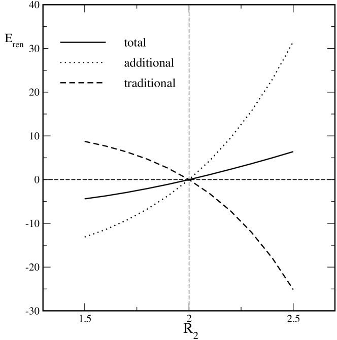
Figure 1: Difference in renormalized energy between shells of radii $R_{2}$ and $R_{1}$, as a function of $R_{2}$ for $R_{1}=2$.

A further complication arises because we require the Hankel functions numerically for any order and any argument. Standard algorithms Press et al. (1992) are not appropriate for very large order and very small arguments. To bypass this obstacle, we use those algorithms only to find $\xi_{\ell}(z)$ for $z\to\infty$ as a boundary value, and then solve the non–linear first order differential equation

$$\frac{d\xi_{\ell}(z)}{dz}=\xi_{\ell}^{2}(z)-1-\frac{\ell(\ell+1)}{z^{2}}$$ (27)

to determine the logarithmic derivative of the spherical Riccati–Hankel function for real $z$. Similarly, we do not use standard algorithms to find the free Green’s function, but rather supplement the set of differential equations (22) by the case $V_{i\kappa}(r)\equiv 0$, which yields $h^{(0)}_{\kappa,\ell}(r)$ with $|\psi^{(0)}_{i\kappa,\ell}|^{2}=\frac{\kappa}{2\ell+1}h^{(0)}_{\kappa,\ell}(r)$. The numerical results presented here are based on Fortran codes. Those programs have also been tested against Mathematica codes for moderate $\ell_{\rm max}$ and $\kappa_{\rm max}$.

In order to make the numerical calculation tractable, we choose moderate values of the model and ansatz parameters, rather than attempting to closely model a physical metallic sphere. Our results, however, are representative of the generic behavior of the stress on a dielectric shell. We work in units where $\lambda_{p}=2$ and choose as our reference contribution a shell with $R_{1}=2$ and $s_{1}=4$ in these units.

Figure 1 shows the results for the choice $\sigma_{p}=2$. We have also studied larger conductivities ($\sigma_{p}=4$ and $\sigma_{p}=8$) and find the same behavior, indicating that the choice of infra–red regularization is not crucial. We find that the traditional contribution, i.e. the one solely based on the phase shift (or equivalently, the logarithm of the Jost function Bordag and Khusnutdinov (2008)), decreases with increasing radii, which would indeed lead to a repulsive self–stress if it were the sole contribution. On the other hand, the additional contribution due to the energy dependence of the dielectric, which is localized at the shell and depends on its material properties, is attractive. In total, the contribution from the additional term overcomes the standard repulsion and we find the electromagnetic Casimir stress of a spherical dielectric shell to be attractive, in agreement with the generic behavior of electromagnetic Casimir forces between rigid bodies, as has been established for configurations with mirror symmetry Kenneth and Klich (2006) and many other geometries (see for example Ref. Rahi et al. (2009)).

Our result shows how the attractive Casimir stress on a dielectric shell arises from a term that is not captured by the idealized boundary condition calculation. The additional contribution clearly originates from the frequency dependence of the dielectric and therefore is a manifestation of material properties. Because the dominant contribution originates in terms in $V^{\hbox{\tiny TM}}_{k}(r)$ proportional to space derivatives of $\epsilon_{k}(r)$, this result nonetheless persists in any limit in which the dielectric approaches such a boundary. We expect this behavior to apply to other cases for which the ideal boundary suggests a repulsive stress, such as a rectangular box, again in agreement with the results from Casimir forces Hertzberg et al. (2005), although it is more difficult to formulate the numerical calculation in that case.