Protein folding: Complex potential for the driving force in a two-dimensional space of collective variables

Abstract

Using the Helmholtz decomposition of the vector field of folding fluxes in a two-dimensional space of collective variables, a potential of the driving force for protein folding is introduced. The potential has two components. One component is responsible for the source and sink of the folding flows, which represent, respectively, the unfolded states and the native state of the protein, and the other, which accounts for the flow vorticity inherently generated at the periphery of the flow field, is responsible for the canalization of the flow between the source and sink. The theoretical consideration is illustrated by calculations for a model $\beta$-hairpin protein.

1 Introduction

Protein folding is a reaction in which a protein attains its functional (native) state; the unfolded state of the protein plays a role of the reactant, and the native state plays a role of the product. In contrast to simple chemical reactions, where the reactant, transition state and product are well defined species, the folding reaction is characterized by ensembles of unfolded and transition states. Accordingly, folding pathways are numerous and diverse. The understanding of this difference between the protein folding and chemical reactions has led to a statistical view of protein folding BryngelsonWolynes87 ; ShakhnovichFarztdinovGutinKarplus91 ; LeopoldMontalOnuchic92 ; BryngelsonOnuchicSocciWolynes95 ; DillChan97 ; Shakhnovich97 ; OnuchicLuthey_SchultenWolynes97 ; DobsonSaliKarplus98 ; DSSDK00 ; SheaBrooks01 ; SchulerEverettLipmanEaton02 ; Gruebele2002 ; MelloBarrick04 ; Karplus11 (for review, see Refs. OnuchicLuthey_SchultenWolynes97, ; DobsonSaliKarplus98, ; DSSDK00, ; SheaBrooks01, and DillOzkanShellWeikl08, ; DillMacCallum12, ; FinkelsteinPtitsyn02, ). According to this view, the folding process is governed by the interplay of the protein potential energy and conformation entropy, forming a ”funnel-like” energy surface. The energy and entropy both decrease from the unfolded states of the protein to its native state but in different manner, so that a free energy barrier is formed that separates the native-like states from the unfolded states.

A tempting and widely used approach to study the folding reaction is to construct a free energy profile as a function of a single reaction coordinate BerezhkovskiiSzabo05 ; RheePande05 ; BestHummer2006 ; KrivovKarplus06 ; BeckDaggett07 ; ChoderaPande11 ; PetersBolhuisMullenShea13 . However, although the diversity of folding pathways is taken into account (as the entropy part of the free energy), this approach is generally limited to the case of a single reaction channel, when the folding pathways can be organized in a ”transition tube” E_Vanden-Eijnden10 . A more powerful method to characterize the diversity of the pathways is the construction of the free energy surface (FES) of the folding reaction as a function of two collective variables SheaBrooks01 ; SocciOnuchicWolynes98 ; BoczkoBrooks95 ; ChekmarevKrivovKarplus05 . One variable is usually chosen to describe the protein compaction during folding (e.g., the radius of gyration, $r_{\mathrm{g}}$), and the other its proximity to the native conformation (e.g., the fraction of the native contacts, $f_{\mathrm{nat}}$). To construct the FES, the probability for the system to be at a current point of the conformation space $P(f_{\mathrm{nat}},r_{\mathrm{g}})$ is calculated and then, using the Boltzmann hypothesis, is converted into the free energy

$$F(f_{\mathrm{nat}},r_{\mathrm{g}})=-k_{\mathrm{B}}T\ln P(f_{\mathrm{nat}},r_{\mathrm{g}})$$ (1)

where $T$ is the temperature, and $k_{\mathrm{B}}$ is the Boltzmann constant. A shortcoming of the FES thus determined is that it does not show the direction of the motion, i.e., the protein can have the same probability to be at some point of the conformation space when it goes towards the native state or requires partial unfolding to reach the native state. To gain a closer insight into folding dynamics, we have recently introduced a ”hydrodynamic” description of the folding process ChekmarevPalyanovKarplus08 . In this approach, similar to the FESs, the folding process is considered in a reduced space of collective variables, and, similar to Markov state models (MSMs) Schutte99 ; SwopePiteraSuits04 ; WeberPande11 , disconnectivity graphs (DGs) BeckerKarplus97 ; KrivovKarplus04 ; Wales03 and protein folding networks (PFNs) RaoCaflisch04 ; Noe-Weikl ; BowmanVoelzPande11 , the calculated folding trajectories are used to determine probabilities of transitions between the protein states. On the one hand, in comparison to the MSMs, this allows consideration of more complex (non-Markovian) kinetics, and on the other, in comparison to the DGs and PFNs, to arrange the protein states according to their distribution in the conformation space KalginCaflischChekmarevKarplus13 . The probabilities of transitions are organized as local flows between the points of the (reduced) conformation space. Given the flows, it is possible to construct the vector field and streamlines of the folding flows, similar to how it is done in hydrodynamics LandauLifshitz87 . Then, the process of protein folding can be viewed as a motion of a folding ”fluid”, with the density of the fluid being proportional to the probability for the system to be at the current point of the conformation space. In equilibrium conditions, the local flows of transitions become small, or vanish, due to detailed balance KalginCaflischChekmarevKarplus13 . Therefore, the hydrodynamic description is most efficient for nonequilibrium conditions, particularly if detailed balance is absent on the overall scale. Such is the case when the native state is essentially stable; then the unfolding events are rare, and the process of folding is reduced to the first-passage folding. Correspondingly, the folding reaction is represented by a steady flow of the folding fluid from the unfolded states of the protein to its native state. For the equilibrium conditions, when the protein repeatedly folds and unfolds, the segments of the equilibrium trajectory between these states can be selected for the first-passage paths from the unfolded to native state, as, for example, in the transition-path theory (TPT) E_Vanden-Eijnden06 ; E_Vanden-Eijnden10 .

The hydrodynamic approach has been successfully applied to the study of folding dynamics of several model proteins - an $\alpha$-helical hairpin (a lattice model) ChekmarevPalyanovKarplus08 , a SH3 domain (a C_α model) KalginKarplusChekmarev09 ; KalginChekmarev11 , and beta3s-miniprotein (all-atom simulations) KalginCaflischChekmarevKarplus13 . It has been found that although the general behavior of the folding flow is consistent with the FES landscape, i.e., the flow is directed from the unfolded states to the native state and mostly concentrated at the bottom of the valley that connects these states, the distribution of the local flows is very different from what the FES suggests ChekmarevPalyanovKarplus08 ; KalginKarplusChekmarev09 . Moreover, local flow vortices can be formed that do not necessarily leave fingerprints on the FES ChekmarevPalyanovKarplus08 ; KalginKarplusChekmarev09 ; KalginChekmarev11 ; KalginCaflischChekmarevKarplus13 , and such vortical flows can have many properties of turbulent flows of a fluid KalginChekmarev11 . In other words, the FES does not present a true potential for folding flows.

The knowledge of the local flows offers a possibility to determine such a potential on the basis of the Helmholtz decomposition ArfkenWeber95 of the vector field of the flows. In the present paper, considering the first-passage folding of a model $\beta$-hairpin protein taken as an example, we show that this potential intrinsically has two components. One component is responsible for the source and sink of the folding flow and the other for the canalization of the flow between the source and sink.

The paper is organized as follows. Section 2 describes the protein model, the simulation method, the hydrodynamic approach, and the choice of collective variables. Also, it presents some results of the simulations to show that the present protein model leads to a representative picture of protein folding (the FES as a function of $f_{\mathrm{nat}}$ and $r_{\mathrm{g}}$, the mean first-passage time as a function of temperature, and the distribution of the first-passage times). Section 3 presents the main results of the work and their discussion: the FES and the vector flow field in the collective variables (3.1), the potential functions for folding fluxes (3.2), and the interpretation of these functions (3.3). Section 4 summarizes the results of the work.

2 Protein Model, Simulation Method and Preliminary Results

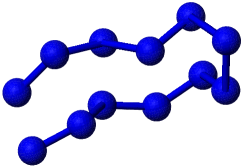
Determining the potential with the Helmholtz decomposition requires a smooth vector field of folding flows and, accordingly, a large number of folding trajectories to be simulated. To perform simulations at a reasonable cost, we considered a short fast-folding protein in the framework of a minimalist model. The goal was to have a representative picture of the folding dynamics rather than to describe folding of a particular protein. Specifically, a twelve-residue $\beta$-hairpin protein 2evq 2evq (Fig. 1) was chosen as a model system, and the interactions between the residues were characterized using a C_α-based Gō-like model, i.e., the residues were represented by monomers (beads) centered at the C_α atoms, with the interaction between the monomers determined by the structure of the native state of the protein Go83 . Specifically, the interaction potential of Ref. HoangCieplak00, was used

$$U=\sum_{1}^{N-1}[k_{1}(r_{i,i+1}-d_{0})^{2}+k_{2}(r_{i,i+1}-d_{0})^{4}]$$

$$+\sum_{i+1<j}^{\mathrm{NAT}}4\varepsilon\left[\left(\frac{\sigma_{ij}}{r_{ij}}\right)^{12}-\left(\frac{\sigma_{ij}}{r_{ij}}\right)^{6}\right]$$

$$+\sum_{i+1<j}^{\mathrm{NON}}4\varepsilon\left[\left(\frac{\sigma_{0}}{r_{ij}}\right)^{12}-\left(\frac{\sigma_{0}}{r_{ij}}\right)^{6}+\frac{1}{4}\right]\Delta(r_{ij}-d_{\mathrm{nat}})$$

where $N$ is the number of monomers (residues), $r_{ij}$ is the current distance between two monomers $i$ and $j$, and $\varepsilon$ is the characteristic attractive energy. The first term represents rigidity of the backbone; here $d_{0}=3.8$Å, $k_{1}=\varepsilon/{\text{\AA}}^{2}$, and $k_{2}=100\varepsilon/{\text{\AA}}^{4}$. The second and third terms describe contributions of the native and non-native contacts, respectively. The contact between two monomers $i$ and $j$ was considered as a native contact if $|j-i|>1$ and the distance between these monomers in the native state was less than 7.5Å. In the second term $\sigma_{ij}=2^{1/6}d_{ij}$, where $d_{ij}$ is the distance between monomers $i$ and $j$ in the native state, and in the third term $d_{\mathrm{nat}}=\langle d_{ij}\rangle$, $\sigma_{0}=2^{1/6}d_{\mathrm{nat}}$, and $\Delta(r_{ij}-d_{\mathrm{nat}})$ is the cutoff function which is equal to 1 for $r_{ij}<d_{\mathrm{nat}}$ and 0 otherwise. The number of native contacts is equal to 27.

The simulations were performed using a constant-temperature molecular dynamics based on the Langevin equation

$$m\frac{d^{2}\mathbf{r}_{i}}{dt^{2}}+\gamma\frac{d\mathbf{r}_{i}}{dt}=-\frac{\partial U}{\partial\mathbf{r}_{i}}+\mathbf{\Phi}_{i}(t)$$ (2)

where $\mathbf{r}_{i}$ is the radius-vector of $i$ monomer representing a residue, $m$ is the monomer mass, $U$ is the potential energy of the system, $\mathbf{\Phi}_{i}$ is a random force from the surroundings (a solvent that is not considered explicitly), and $\gamma$ is the friction coefficient that introduces viscosity of the surroundings to balance the random force and dissipation. The random forces have the Gaussian distribution with zero mean and variance $\langle\Phi_{i}^{j}(t)\Phi_{i^{\prime}}^{j^{\prime}}(t+\tau)\rangle=2\gamma k_{\mathrm{B}}T\delta_{ii^{\prime}}\delta_{jj^{\prime}}\delta(\tau)$, where the angular brackets denote an ensemble average, the upper index at $\Phi$ stands for the vector component, and $\delta_{kk^{\prime}}$ and $\delta(\tau)$ are the Kronecker and Dirac delta functions, respectively. The equation was numerically integrated using the algorithm of Ref. BiswasHamann86, with the time step $\Delta t=0.005\tau$ and $\gamma=3m/\tau$. With the length scale $l=7.5$Å and the attractive energy $\varepsilon\sim 1{\mathrm{kcal/mol}}$, the characteristic time scale $\tau=(ml^{2}/\varepsilon)^{1/2}$ is $\sim 1$ps, where $m$=110 Da.

To characterize protein conformations, we employed a set of the bond distances between the monomers which are not immediate neighbors along the protein chain; they formed a 55-dimensional conformation space. Using the principal component analysis (PCA) Jolliffe02 , this space was reduced to a two-dimensional space of collective variables $\mathbf{g}=(g_{1},g_{2})$. The variable $g_{1}$ was directed along the eigenvector for the largest eigenvalue, and the variable $g_{2}$ along the vector calculated as the linear combination of the rest of the eigenvectors, which contributed with the weights corresponding to their eigenvalues. Although the second principal component could also be chosen as $g_{2}$, because the first two eigenvalues are well separated from the others (Fig. 2), the present choice makes it possible to take into account the effects missed by the first component.

The hydrodynamic description of protein folding ChekmarevPalyanovKarplus08 is based on the calculation of the transitions in a space of collective variables (the space $\mathbf{g}$ in the present case). These transitions are organized into transition probability local flows (fluxes) $\mathbf{j(g)}$. In the case of two variables, $\mathbf{g}=(g_{1},g_{2})$, the $g_{1}$-component of the flux at a point $\mathbf{g}$ is determined as

$$j_{g_{1}}({\bf g})=[\sum^{{g_{1}}^{\prime\prime}-{g_{1}}^{\prime}>0}_{{\bf g^{\prime}},{\bf g^{\prime\prime}}({\bf g}\subset{\bf g}^{\ast})}n({\bf g^{\prime\prime}},{\bf g^{\prime}})$$

$$-\sum^{{g_{1}}^{\prime\prime}-{g_{1}}^{\prime}<0}_{{\bf g^{\prime}},{\bf g^{\prime\prime}}({\bf g}\subset{\bf g}^{\ast})}n({\bf g^{\prime\prime}},{\bf g^{\prime}})]/(M\bar{t}_{\mathrm{f}})$$ (3)

where $M$ is the total number of simulated trajectories, $\bar{t}_{\mathrm{f}}$ is the mean first-passage time (MFPT), $n({\bf g^{\prime\prime}},{\bf g^{\prime}})$ is the number of transitions from state ${\bf g^{\prime}}$ to ${\bf g^{\prime\prime}}$, and ${\bf g}\subset{\bf g}^{\ast}$ is a symbolic designation of the condition that the transitions included in the sum have the straight line connecting points ${\bf g^{\prime}}$ to ${\bf g^{\prime\prime}}$, which crosses the line $g_{1}={\mathrm{const}}$ within the segment of the length of $\Delta g_{2}$ centered at the point ${\bf g}$. The $g_{2}$-component of ${\bf j}(\bf{g})$ is determined in a similar way, except that one selects the transitions crossing the line ${g_{2}}={\mathrm{const}}$. The calculations were performed on a grid with discretization $\Delta g_{1}=\Delta g_{2}=0.12$.

There were simulated $1\times 10^{4}$ folding trajectories at a temperature equal to $T=0.17$ (in units $\varepsilon/k_{\mathrm{B}}$, where $k_{\mathrm{B}}$ is the Boltzmann constant). Each trajectory started at an unfolded state of the protein and was terminated upon reaching the native state. The unfolded states were prepared by thermalization of the native conformation at $T=0.5$ for $1\times 10^{4}$ time steps; if the number of native contacts did not exceed 4, the conformation was accepted, if exceeded, the thermalization was continued. The native state was considered to be reached when the root-mean square deviation (RMSD) of the protein conformation from the native conformation was less than 1Å.

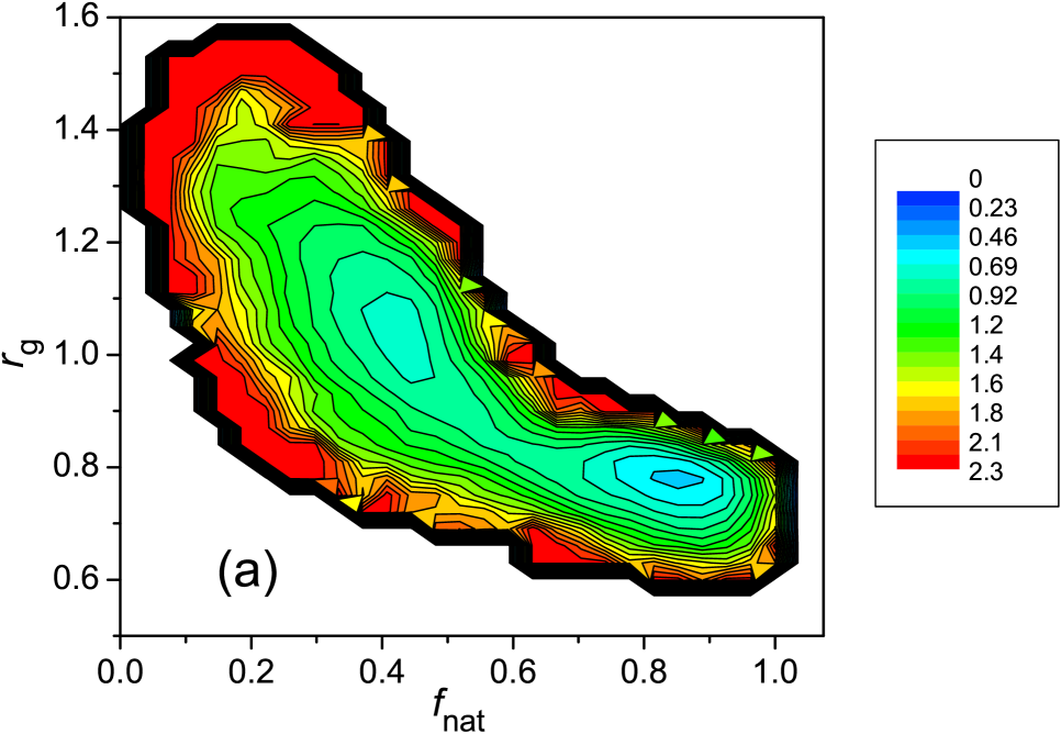
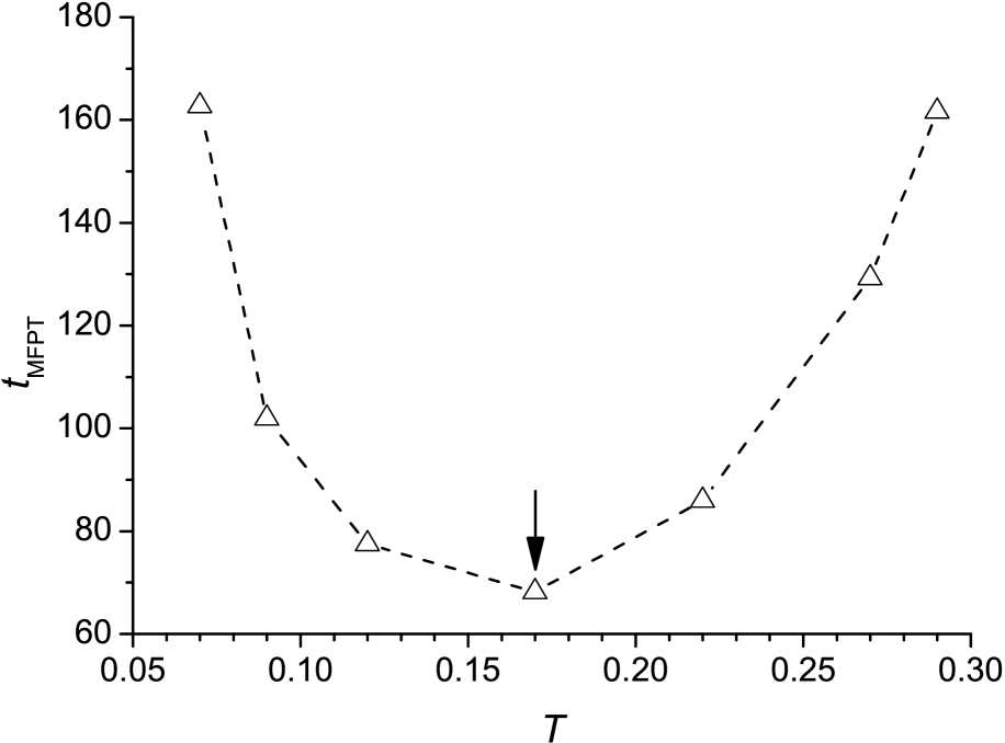
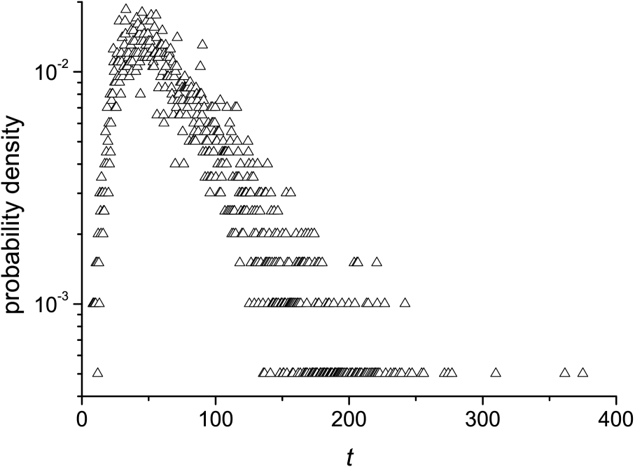
The simulations have shown that the given protein model provides a sufficiently representative picture of protein folding, both from the ”thermodynamic” and kinetic viewpoints. The FES calculated as a function of the fraction of native contacts and the radius of gyration is ”L-shaped”, which is characteristic of a wide family of proteins in which an early collapse is observed SheaBrooks01 , including beta-proteins PandeRokhsar99 ; DinnerLazaridisKarplus99 (Fig. 3), the dependence of the MFPT on the temperature exhibits the well-known U-shape behavior found in experiments and simulations OlivebergYanFersht95 ; Karplus97 ; ChekmarevKrivovKarplus05 (Fig. 4), and the folding kinetics are essentially single-exponential at the ”optimal” folding temperature at which the MFPT has the minimum value ChekmarevKrivovKarplus05 (Fig. 5).

3 Results and Discussion

3.1 Free Energy Surface and Folding Flow Field in the PCA Variables

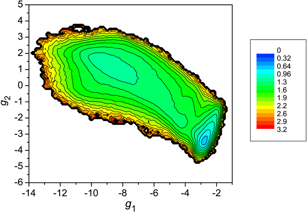
The FES as a function of the collective PCA variables $g_{1}$ and $g_{2}$ is shown in Fig. 6. It was calculated similar to the above shown FES in ”physical” variables (Fig. 3), i.e., using the equation similar to Eq. (1). The FES has a characteristic ”bean-like” shape typically observed if one employs the PCA coordinates as the collective variables, e.g., Refs. KrivovKarplus04, and LevyJortnerBecker01, . At the same time, the present FES retains two essential properties of the FES of Fig. 3, in that the global landscape of the surface has the form of a valley connecting the unfolded states and the native state, and there exists a free energy barrier separating these states.

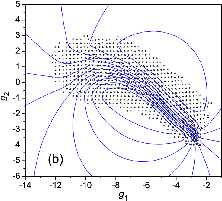
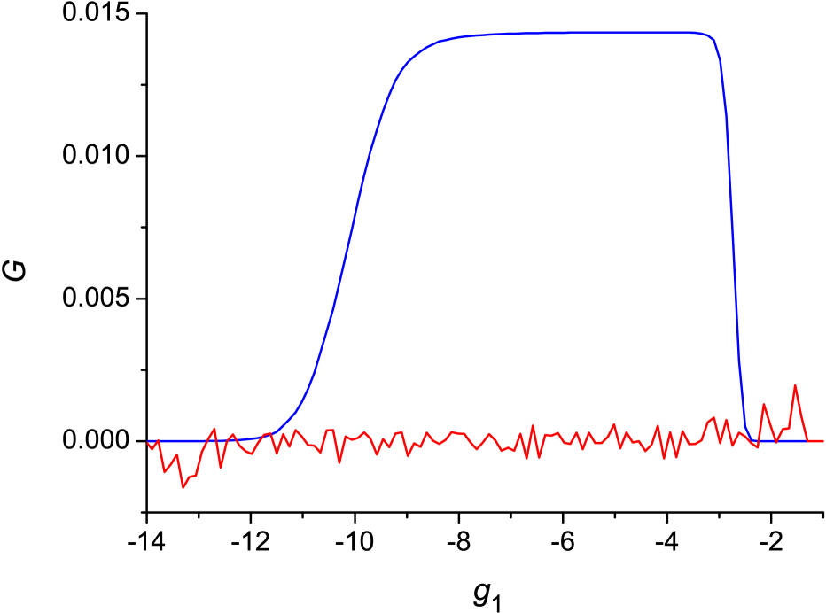
Figure 7$\bf{a}$ depicts the distribution of $\mathbf{j(g)}$ in the form of vector field (for illustrative purpose, the lengths of the vectors are equally increased by factor $3.5\times 10^{2}$). As is seen from the comparison of Fig. 7$\bf{a}$ with Fig. 6, the flow field lies within the free energy valley that connects the unfolded states to the native state, and the flow is concentrated at the bottom of the valley. Integration of the $g_{1}$-component of $\mathbf{j(g)}$ over $g_{2}$ in each cross-section $g_{1}={\mathrm{const}}$ shows that the total flow from the unfolded states to the native state, $G(g_{1})=\int j_{g_{1}}(g_{1},g_{2})dg_{2}$, is essentially constant in the region between the source and sink of the flow (Fig. 8).

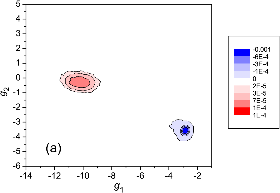
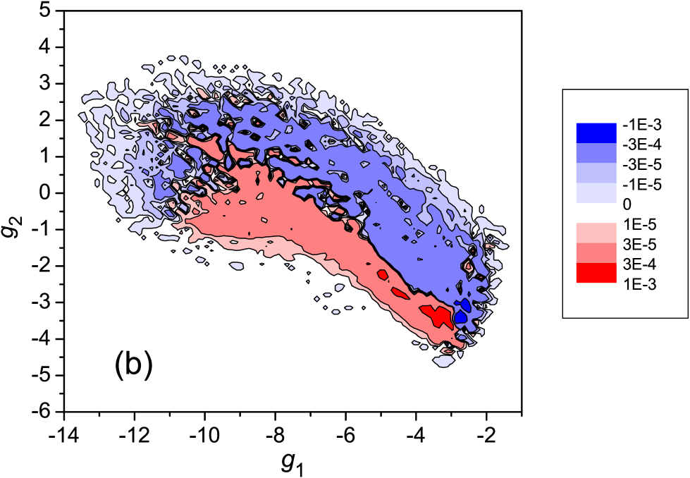
Figure 9 shows how the divergence of the folding flow ($q=\partial j_{g_{1}}/\partial g_{1}+\partial j_{g_{2}}/\partial g_{2}$, panel a) and its vorticity ($\omega=\partial j_{g_{2}}/\partial g_{1}-\partial j_{g_{1}}/\partial g_{2}$, panel b) are distributed in the $(g_{1},g_{2})$ space. Except for two localized regions at the unfolded and native states, which represent, respectively, the source and sink of the folding flow, the flow is divergence-free. The vorticity, in contrast, spans the entire flow field. It arises because the intensity of the flow decreases towards both sides of the free energy valley (Fig. 7$\bf{a}$); correspondingly, the vorticity has different signs on the different sides of the valley (see the above equation for vorticity). This decrease of the flow intensity towards the valley sides is a natural phenomenon, because the lower the probability to visit some region of the conformation space (in the present case, a side of the valley), the smaller the flows in this region; similar nonuniform distributions of the flows have been previously observed for an $\alpha$-helical hairpin ChekmarevPalyanovKarplus08 and SH3 domain KalginKarplusChekmarev09 . Therefore, the vorticity generated on the periphery of the folding flow field presents an intrinsic property of the folding dynamics.

Comparison of Fig. 7$\bf{a}$ to Fig. 6 shows that the folding flux distribution is consistent with the FES landscape in that the overall folding flow follows the valley of the FES that connects the unfolded states to the native state. At the same time, the corresponding free energy $F(\mathbf{g})$ does not present a true potential of folding fluxes, i.e., determining the fluxes as $j_{g_{1}}=-\partial F(\mathbf{g})/\partial g_{1}$ and $j_{g_{2}}=-\partial F(\mathbf{g})/\partial g_{2}$ leads to a vector flow field drastically different from that of Fig. 7$\bf{a}$ (Fig. 10). Calculation of the corresponding total flow shows that the flow is not constant but fluctuates around zero value (Fig. 8).

3.2 Potentials for Folding Fluxes

To determine an actual potential for the folding fluxes, we use the Helmholtz decomposition theorem ArfkenWeber95 , according to which any smooth vector field can be uniquely represented as a sum of two terms: a curl-free field and a divergence-free field. Then

$$\mathbf{j}={\mathbf{j}}_{\mathrm{cf}}+{\mathbf{j}}_{\mathrm{df}}$$ (4)

where ${\mathbf{j}}_{\mathrm{cf}}$ is the curl-free component, and ${\mathbf{j}}_{\mathrm{df}}$ is the divergence-free component, i.e., $\nabla\times{\mathbf{j}}_{\mathrm{cf}}=0$ and $\nabla\cdot{\mathbf{j}}_{\mathrm{df}}=0$, respectively. These conditions allow introducing the potentials of the vector fields. In the case of two dimensions, vectors ${\mathbf{j}}_{\mathrm{cf}}$ and ${\mathbf{j}}_{\mathrm{df}}$ can be written as

$${\mathbf{j}}_{\mathrm{cf}}=-\frac{\partial\Phi}{\partial g_{1}}{\mathbf{k}}_{1}-\frac{\partial\Phi}{\partial g_{2}}{\mathbf{k}}_{2}$$ (5)

$${\mathbf{j}}_{\mathrm{df}}=\frac{\partial\Psi}{\partial g_{2}}{\mathbf{k}}_{1}-\frac{\partial\Psi}{\partial g_{1}}{\mathbf{k}}_{2}$$

where $\Phi=\Phi({\mathbf{g}})$ is the potential for the curl-free component, $\Psi=\Psi({\mathbf{g}})$ is the potential for the divergence-free component, and ${\mathbf{k}}_{1}$ and ${\mathbf{k}}_{2}$ are the unit vectors for the variables $g_{1}$ and $g_{2}$, respectively. The sets of the equipotential lines $\Phi(\mathbf{g})=\mathrm{const}$ and $\Psi(\mathbf{g})=\mathrm{const}$ are not mutually orthogonal because $\nabla\Psi\cdot\nabla\Phi=\partial\Psi/\partial g_{1}\cdot\partial\Phi/\partial g_{1}+\partial\Psi/\partial g_{2}\cdot\partial\Phi/\partial g_{2}$ is generally nonzero. This is the effect of the flow vorticity: if the flow were both divergence- and curl-free, the flow flux ${\mathbf{j}}$ could be written in either form of Eq. (5). Then, the potential functions $\Phi({\mathbf{g}})$ and $\Psi({\mathbf{g}})$ would satisfy the relations $\partial\Psi/\partial g_{2}=-\partial\Phi/\partial g_{1}$ and $\partial\Psi/\partial g_{1}=\partial\Phi/\partial g_{2}$ characteristic of the potential flows (the Cauchy-Riemann conditions) LandauLifshitz87 , in which case $\nabla\Psi\cdot\nabla\Phi=0$.

Substituting the given expressions for ${\mathbf{j}}_{\mathrm{cf}}$ and ${\mathbf{j}}_{\mathrm{df}}$ into Eq. (4) and regrouping the terms, one obtains

$$\mathbf{j}=j_{g_{1}}{\mathbf{k}}_{1}+j_{g_{2}}{\mathbf{k}}_{2}$$

where

$$j_{g_{1}}=-\frac{\partial\Phi}{\partial g_{1}}+\frac{\partial\Psi}{\partial g_{2}},\hskip 14.22636ptj_{g_{2}}=-\frac{\partial\Phi}{\partial g_{2}}-\frac{\partial\Psi}{\partial g_{1}}$$ (6)

To find functions $\Phi(\mathbf{g})$ and $\Psi(\mathbf{g})$, the functional

$$Q=\int[\left(j_{g_{1}}+\frac{\partial\Phi}{\partial g_{1}}-\frac{\partial\Psi}{\partial g_{2}}\right)^{2}$$

$$+\left(j_{g_{2}}+\frac{\partial\Phi}{\partial g_{2}}+\frac{\partial\Psi}{\partial g_{1}}\right)^{2}]dg_{1}dg_{2}$$ (7)

was minimized with respect to $\Phi(\mathbf{g})$ and $\Psi(\mathbf{g})$; here $j_{g_{1}}$ and $j_{g_{2}}$ are the folding fluxes obtained with the molecular dynamics simulations. Integration in Eq. (3.2) was performed numerically on a grid with the same discretization as for Eq. (2). To avoid boundary effects, the region of integration was extended to $-21.8\leq g_{1}\leq 7.0$ and $-13.7\leq g_{2}\leq 12.7$ (cf. Fig. 6). At the boundaries of the region, no-flux conditions were imposed, i.e., at the left and right boundaries ($g_{1}=\mathrm{const}$) it was assumed $j_{g_{1}}=0$, and at the lower and upper boundaries ($g_{2}=\mathrm{const}$) $j_{g_{2}}=0$. The minimization was performed using the steepest-descent method with a variable step-size. Starting with $\Phi(\mathbf{g})=\Psi(\mathbf{g})=0$ as an initial guess for these functions, in which case $Q\approx 1\times 10^{-3}$, the process was continued until $Q$ was as small as $\approx 1\times 10^{-11}$, i.e., even in the worst case, when the deviation of the fluxes determined by Eqs. (6) from the fluxes obtained in the simulations was concentrated at a single point, it would not exceed $\sim 0.01\%$.

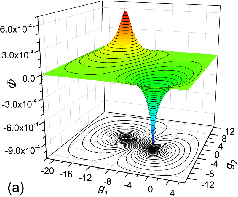
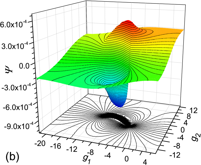
The results of the calculations are shown in Fig. 11. In agreement with the Helmholtz decomposition ArfkenWeber95 , the functions $\Phi(\mathbf{g})$ and $\Psi(\mathbf{g})$ are characteristically different in that the former accounts for the source and sink of the flows, and the latter for the vorticity effects. More specifically, as can be seen from comparison of Eq. (6) with Fig. 11, the function $\Phi(\mathbf{g})$ determines the intensity of the flow in the vicinity of the source and sink, and the function $\Psi(\mathbf{g})$ determines it in the region between the source and sink, providing the canalization of the flow within the free energy valley that connects the unfolded states to the native state. Thus, both functions, $\Phi(\mathbf{g})$ and $\Psi(\mathbf{g})$, are equally important for a correct description of the folding dynamics and should be considered as the intrinsic components of the complex potential that determines the driving force.

3.3 Interpretation of the Potentials

In hydrodynamic terms LandauLifshitz87 , the functions $\Phi(\mathbf{g})$ and $\Psi(\mathbf{g})$ can be associated, respectively, with the scalar potential of the flow and the vector potential, or more specifically, with the component of the vector potential that is orthogonal to the two-dimensional plane under consideration. The latter plays a role of the stream function, for which the equation $\Psi(\mathbf{g})=\mathrm{const}$ determines the streamline of the flow, i.e., the line that is tangent to the local directions of the $\mathbf{j(g)}$ vectors (Fig. 7$\bf{b}$). The difference between the stream functions for two streamlines determines the fraction of the total flow in the stream tube between the streamlines (see also Refs. ChekmarevPalyanovKarplus08, and KalginKarplusChekmarev09, ). Similar to a steady potential flow of an inviscid fluid in a two-dimensional space LandauLifshitz87 , the functions $\Phi(\mathbf{g})$ and $\Psi(\mathbf{g})$ can also be written as a complex function $\Theta({\mathbf{g}})=\Phi(\mathbf{g})+i\Psi(\mathbf{g})$, where $i$ is the imaginary unit; then ${\mathbf{j}}({\mathbf{g}})=j_{g_{1}}+ij_{g_{2}}=-\nabla_{c}\Theta({\mathbf{g}})$, where $\nabla_{c}=\partial/\partial g_{1}+i\partial/\partial g_{2}$ is the gradient operator in the complex number space $(g_{1},ig_{2})$. However, in contrast to the potential flow of inviscid fluid, the function $\Theta({\mathbf{g}})$ is not analytic function, i.e., is not a function of complex variable $g_{1}+ig_{2}$, because the Cauchy-Riemann conditions, which represent the necessary and sufficient condition for a function to be analytic and require the flow to be divergence- and curl-free ArfkenWeber95 , are not satisfied (Fig. 9). Therefore, the methods of the theory of analytic functions of complex variable, which are successfully used in hydrodynamics LandauLifshitz87 , are not applicable here.

Another interpretation of the potentials $\Phi(\mathbf{g})$ and $\Psi(\mathbf{g})$ stems from the kinetic theory Kampen81 . According to Eq. (6), the velocity of motion is proportional to the forces produced by these potentials, i.e., the local flows are assumed to be drift flows. In other words, although the inertia of the monomers was present in the Langevin equation we used for the simulations, the potentials $\Phi(\mathbf{g})$ and $\Psi(\mathbf{g})$ determined from the resulted fluxes $j_{g_{1}}$ and $j_{g_{2}}$ account for an overdamped motion. The approximation of the overdamped motion, which neglects the inertia term in the Langevin equation (2), is rather common to characterize the protein folding dynamics RohrdanzZhengClementi13 . The corresponding kinetic equation is the Smoluchowski equation $\partial p/\partial t+\nabla\cdot\mathbf{J}=0$, where $p(\mathbf{g},t)$ is the probability density, $\nabla$ is the gradient operator in the coordinate space $\mathbf{g}$, and $\mathbf{J}$ is the probability current, which can be written as $\mathbf{J}=-D(\mathbf{g})\nabla p+D(\mathbf{g})/(k_{\mathrm{B}}T){\mathbf{F}}(\mathbf{g})p$, where $-D(\mathbf{g})\nabla p$ is the diffusion flux, $D(\mathbf{g})/(k_{\mathrm{B}}T){\mathbf{F}}(\mathbf{g})p$ is the drift flux, $D(\mathbf{g})$ is the diffusion tensor, and ${\mathbf{F}}(\mathbf{g})$ is the driving force. If the probability current were zero, i.e., detailed balance existed, the equality $\mathbf{J}=0$ would give the equilibrium (Boltzmann) distribution $p(\mathbf{g})\sim\exp[-G(\mathbf{g})]/k_{\mathrm{B}}T$, where $G(\mathbf{g})$ is the free energy that exerts the driving force ${\mathbf{F}}(\mathbf{g})=-\nabla G(\mathbf{g})$. This case would correspond to a curl-free drift flow, with the potential of the driving force being determined by a single function in the form of the free energy $G(\mathbf{g})$. However, if the probability current is nonzero, as in the present case, i.e., when the steady flow from the unfolded state to the native state exists, the stationary solution is determined by the condition $\nabla\cdot\mathbf{J}=0$, so that $\mathbf{J}$ can have a curl component Kampen81 . Such flow is non-equilibrium and is characterized by ”irreversible circulation” or ”cyclic balance”, which can be considered as a measure of deviation from detailed balance TomitaTomita74 ; Graham77 ; EyinkLebowitzSpohn96 . In our case the circulating flow is represented by the flux vector ${\mathbf{j}}_{\mathrm{df}}$ and, according to Eq. (5), is generated by the potential $\Psi(\mathbf{g})$, with the factor $D(\mathbf{g})/(k_{\mathrm{B}}T)$ being included into the potential. In general case, the driving force can be written as $\mathbf{F}=-\nabla\Phi+\nabla\times\mathbf{A}$, where $\Phi$ and $\mathbf{A}$ are the scalar and vector potentials, respectively (in the case of two dimensions, only the component of $\mathbf{A}$ that is orthogonal to the plane is involved). The potentials of this type have recently been used to study the dynamics of Brownian particles in corrugated channels MartensStraubeSchmidSchimansky-GeierHaanggi13 ; AiHeLiZhong13 .

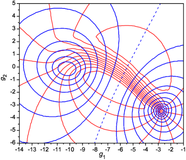
As an anonymous reviewer of the manuscript remarked, the resulting picture of the folding process in terms of the $\Psi$ and $\Phi$ potentials is very similar to the picture obtained for the reaction dynamics in the TPT E_Vanden-Eijnden06 , although the approaches are apparently different. In the latter, the committor probability functions are calculated for the transition paths from the reactant to the product, and the spatial distribution of the probability currents of the reaction paths (fluxes) between these states is determined E_Vanden-Eijnden10 . The currents are normal to the isocommittor surfaces and organized in the form of the reaction tubes that connect the reactant and product wells, so that the boundaries of the tubes represent the flow lines (streamlines) of the currents. Then the equipotential lines $\Psi(\mathbf{g})=\mathrm{const}$ and $\Phi(\mathbf{g})=\mathrm{const}$ (Fig. 12) can be associated with the flow lines and the isocommittor surfaces, respectively. In particular, the line $\Phi(\mathbf{g})=0$, shown by the dashed curve, which separates the source and sink regions of the flow, can play a role of the isocommittor surface of probability of 1/2. Very interesting from physical and methodological viewpoints, this analogy, however, does not probably extend beyond qualitative resemblance because, in contrast to the flow lines and the isocommittor surfaces, the sets of the equipotential lines $\Phi(\mathbf{g})=\mathrm{const}$ and $\Psi(\mathbf{g})=\mathrm{const}$ are not mutually orthogonal (as has been previously indicated). As is seen from Fig. 12, they possess the orthogonality property only approximately.

4 Conclusions

In summary, we have shown that the potential of the driving force for protein folding in a two-dimensional space of collective variables has two components. One component accounts for the source and sink of the folding flow, representing, respectively, the unfolded and native states of the protein, and the other accounts for the vorticity generated at the periphery of the flow field and provides the canalization of the flow within the free energy valley that connects the unfolded and native states. Since the Helmholtz decomposition theorem ArfkenWeber95 guarantees that any vector field can be uniquely represented by a sum of divergence-free and curl-free fields, the present approach is equally applicable to more complex folding dynamics that are characterized by multiple reaction channels and formation local vortices of the folding flows, as, for example, for folding of SH3 domain KalginKarplusChekmarev09 ; KalginChekmarev11 . In this case, the functions $\Phi(\mathbf{g})$ and $\Psi(\mathbf{g})$ will be not as regular as in Fig. 11 because they should take into account this additional complexity of the folding flow, but the general pattern of these functions is expected to be preserved because of the presence of the source and sink of the folding flow and its vorticity inherently generated at the periphery of the flow field. The requirement of smoothness of the vector field, which is necessary for the Helmholtz decomposition ArfkenWeber95 , currently restricts the possibilities of analysis of folding of proteins of practical interest on atomic level of resolution, however, for small proteins, such, e.g., as the beta3s miniprotein, the calculation of smooth vector fields is quite feasible KalginCaflischChekmarevKarplus13 . Also note that the application of the present approach is not limited to the case of the folding reaction. Similar complex potentials can be expected for other systems that involve multiple reaction pathways, e.g., for nanoclusters, in which the transition between the structures of alternative morphology is characterized by a multi-funnel energy landscape Wales03 .

5 Acknowledgments

I would like to thank an anonymous reviewer for the remark on the similarity between the hydrodynamic and TPT pictures of the reaction.

Figure 1: The ”bead” model of the native conformation of the 2evq de novo protein 2evq .

Figure 2: Spectrum of eigenvalues.

Figure 3: The free energy surface as a function of the fraction of native contacts and radius of gyration, $T=0.17$.

Figure 4: The mean first-passage time as a function of temperature. The arrow indicates the temperature ($T=0.17$) at which the study was performed.

Figure 5: The distribution of the first-passage times, $T=0.17$.

Figure 6: Free energy surface as a function of collective variables $g_{1}$ and $g_{2}$.

Figure 7: Vector field of folding fluxes: ($\bf{a}$) the vector field, and ($\bf{b}$) the streamlines $\Psi(\mathbf{g})=\mathrm{const}$ (blue lines) superimposed on the vector field. The fraction of the total flow in a stream tube between two neighboring streamlines is equal to 0.1.

Figure 8: The total flow from the unfolded states to the native state as a function of the longitudinal variable $g_{1}$. The blue curve depicts the total flow as it was obtained in the simulations. The product of the maximum value of the flow ($G\approx 1.4338\times 10^{-2}$) by the MFPT ($t_{\mathrm{f}}\approx 69.7368$) is close to 1 with very good accuracy. The red curve shows the total flow calculated from the fluxes of Fig. 10; the value of the flow is reduced by $1\times 10^{4}$ times.

Figure 9: The distributions of the ($\bf{a}$) divergence and ($\bf{b}$) vorticity of the folding fluxes.

Figure 10: Vector flow field calculated from the FES of Fig. 3 with the fluxes determined as $j_{g_{1}}=-\partial F(\mathbf{g})/\partial g_{1}$ and $j_{g_{2}}=-\partial F(\mathbf{g})/\partial g_{2}$, where $F(\mathbf{g})$ is the free energy function of Fig. 3.

Figure 11: The functions $\Phi(g_{1},g_{2})$ (panel $\bf{a}$) and $\Psi(g_{1},g_{2})$ (panel $\bf{b}$).

Figure 12: The sets of the equipotential lines $\Phi(g_{1},g_{2})={\mathrm{const}}$ (blue color) and $\Psi(g_{1},g_{2})={\mathrm{const}}$ (red color) corresponding to Fig. 11. The dashed line is for $\Phi(g_{1},g_{2})=0$.

References

- (1) J. D. Bryngelson and P. G. Wolynes, Proc. Natl. Acad. Sci. USA 84, 7524 (1987).
- (2) E. Shakhnovich, G. Farztdinov, A. M. Gutin, and M. Karplus, Phys. Rev. Lett. 67, 1665 (1991).
- (3) P. E. Leopold, M. Montal, and J. N. Onuchic, Proc. Natl. Acad. Sci. USA 89, 8721 (1992).
- (4) J. D. Bryngelson, J. N. Onuchic, N. D. Socci, and P. G. Wolynes, Proteins: Structure, Function, and Bioinformatics 21, 167 (1995).
- (5) K. A. Dill and H. S. Chan, Nat. Struct, Biol. 4, 10 (1997).
- (6) E. I. Shakhnovich, Curr. Opin. Struct. Biol. 7, 29 (1997).
- (7) J. N. Onuchic, Z. Luthey-Schulten, P. G. Wolynes, Annu. Rev. Phys. Chem. 48, 545 (1997).
- (8) C. M. Dobson, A. S̆ali, and M. Karplus, Angew. Chem. Int. Ed. 37, 869 (1998).
- (9) A. R. Dinner, A. S̆ali, L. J. Smith, C. M. Dobson, and M. Karplus, Trends Biochem. Sci. 25, 331 (2000).
- (10) J.-E. Shea and C. L. Brooks III, Annu. Rev. Phys. Chem. 52, 499 (2001).
- (11) B. Schuler, E. A. Lipman, and W. A. Eaton, Nature 419, 743 (2002).
- (12) M. Gruebele, Curr. Opinion Struct. Biol. 12, 161 (2002).
- (13) C. C. Mello and D. Barrick, Proc. Natl. Acad. Sci. USA 101, 14102 (2004).
- (14) M. Karplus, Nat. Chem. Biol. 7, 401 (2011).
- (15) K. A. Dill, S. B. Ozkan, M. S. Shell, and T. R. Weikl, Annu. Rev. Biophys. 37, 289 316 (2008).
- (16) K. A. Dill and J. L. MacCallum, Science 338, 1042 (2012).
- (17) A. V. Finkelstein and O. Ptitsyn, Protein Physics: A Course of Lectures (Academic Press: London, 2002).
- (18) A. Berezhkovskii and A. Szabo, J. Chem. Phys. 122, 014503 (2005).
- (19) Y. M. Rhee and V. S. Pande, J. Phys. Chem. B 109, 6780 (2005).
- (20) R. B. Best and G. Hummer, Proc. Natl. Acad. Sci. U.S.A. 102, 6732 (2005).
- (21) S. V. Krivov and M. Karplus, J. Phys. Chem. B 110, 12689 (2006).
- (22) D. A. C. Beck and V. Daggett, Biophys. J. 93, 3382 (2007).
- (23) J. D. Chodera and V. S. Pande, Phys. Rev. Lett. 107, 098102 (2011).
- (24) B. Peters, P. G. Bolhuis, R. G. Mullen, and J.-E. Shea, J. Chem. Phys. 138, 054106 (2013).
- (25) W. E and E. Vanden-Eijnden, Annu. Rev. Phys. Chem. 61, 391 (2010).
- (26) E. M. Boczko and C. L. Brooks III, Science 269, 393 (1995).
- (27) N. D. Socci, J. N. Onuchic, and P. G. Wolynes, Proteins: Structure, Function, and Genetics 32, 136 (1998).
- (28) S. F. Chekmarev, S. V. Krivov, and M. Karplus, J. Phys. Chem. B 109, 5312 (2005).
- (29) S. F. Chekmarev, A. Yu. Palyanov, and M. Karplus, Phys. Rev. Lett. 100, 018107 (2008).
- (30) C. Schütte, Habilitation thesis, Department of Mathematics and Computer Science, Freie Universitat Berlin, 1999.
- (31) W. C. Swope, J. W. Pitera, and F. Suits, J. Phys. Chem. B 108, 6571 (2004).
- (32) J. K. Weber and V. S. Pande, J. Chem. Theory Comput. 7, 3405 (2011).
- (33) O. M. Becker and M. Karplus, J. Chem. Phys. 106, 1495 (2007).
- (34) S. V. Krivov and M. Karplus, Proc. Natl. Acad. Sci. U.S.A. 101, 14766 (2004).
- (35) D. J. Wales, Energy Landscapes: Applications to Clusters, Biomolecules and Glasses (Cambridge University Press: Cambridge, 2003).
- (36) F. Rao and A. Caflisch, J. Mol. Biol. 342, 299 (2004).
- (37) F. Noé, C. Schütte, E. Vanden-Eijnden, L. Reich, and T. R. Weikl, Curr. Opin. Struct. Biol. 106, 19011 (2009).
- (38) G. R. Bowman, V. A. Voelz, and V. S. Pande, Proc. Natl. Acad. Sci. USA 21, 4 (2011).
- (39) I. V. Kalgin, A. Caflisch, S. F. Chekmarev, and M. Karplus, J. Phys. Chem. B 117, 6092 (2013).
- (40) L. D. Landau and E. M. Lifshitz, Fluid Mechanics (Pergamon: New York, 1987).
- (41) I. V. Kalgin, M. Karplus, and S. F. Chekmarev, J. Phys. Chem. B 113, 12759 (2009).
- (42) I. V. Kalgin and S. F. Chekmarev, Phys. Rev. E 83, 011920 (2011).
- (43) W. E and E. Vanden-Eijnden, J. Stat. Phys. 123, 503 (2006).
- (44) G. B. Arfken and H. J. Weber, Mathematical Methods for Physicists, 4th ed. (Academic Press: San Diego, 1995).
- (45) N. H. Andersen, K. A. Olsen, R. M. Fesinmeyer, X. Tan, F. M. Hudson, L. A. Eidenschink, and S. R. Farazi, J. Am. Chem. Soc. 128, 6101 (2006).
- (46) N. Gō, Annu. Rev. Biophys. Bioeng. 12, 183 (1983).
- (47) T. X. Hoang and M. Cieplak, J. Chem. Phys. 112, 6851 (2000).
- (48) R. Biswas and D. R. Hamann, Phys. Rev. B 34, 895 (1986).
- (49) I. T. Jolliffe, Principal Component Analysis; 2nd ed. (Springer: New York, 2002).
- (50) V. S. Pande and D. S. Rokhsar, Proc. Natl. Acad. Sci. USA 94, 9062 (1999).
- (51) A. R. Dinner, T. Lazaridis and M. Karplus, Proc. Natl. Acad. Sci. USA 96, 9068 (1999).
- (52) M. Oliveberg, Y.-J. Yan, and A. R. Fersht, Proc. Natl. Acad. Sci. U.S.A. 92, 8926 (1995).
- (53) M. Karplus, Fold. Des. 2, 569 (1997).
- (54) Y. Levy, J. Jortner, and O. M. Becker, Proc. Natl. Acad. Sci. U.S.A. 98, 2188 (2001).
- (55) N. G. van Kampen, Stochastic Processes in Physics and Chemistry (North-Holland: Amsterdam, 1981), p. 294.
- (56) M. A. Rohrdanz, W. Zheng, and C. Clementi, Annu. Rev. Phys. Chem. 64, 295 (2013).
- (57) K. Tomita and H. Tomita, Prog. Theor. Phys. 51, 1731 (1974).
- (58) R. Graham, Z. Phys. B 26, 397 (1977).
- (59) G. L. Eyink, J. L. Lebowitz, and H. Spohn, J. Stat. Phys. 83, 385 (1996).
- (60) S. Martens, A. V. Straube, G. Schmid, L. Schimansky-Geier, and P. Haänggi, Phys. Rev. Lett. 110, 010601 (2013).
- (61) B.-Q. Ai, Y.-F. He, F.-G. Li, and W.-R. Zhong, J. Chem. Phys. 138, 154107 (2013).