A Nonlinear Constrained Optimization Framework for Comfortable and Customizable Motion Planning of Nonholonomic Mobile Robots – Part II

Abstract

In this series of papers, we present a motion planning framework for planning comfortable and customizable motion of nonholonomic mobile robots such as intelligent wheelchairs and autonomous cars. In Part I, we presented the mathematical foundation of our framework, where we model motion discomfort as a weighted cost functional and define comfortable motion planning as a nonlinear constrained optimization problem of computing trajectories that minimize this discomfort given the appropriate boundary conditions and constraints.

In this paper, we discretize the infinite-dimensional optimization problem using conforming finite elements. We describe shape functions to handle different kinds of boundary conditions and the choice of unknowns to obtain a sparse Hessian matrix. We also describe in detail how any trajectory computation problem can have infinitely many locally optimal solutions and our method of handling them. Additionally, since we have a nonlinear and constrained problem, computation of high quality initial guesses is crucial for efficient solution. We show how to compute them.

1 Introduction

In the first paper of this series (Gulati et al.,, 2013), we formulated motion planning for a nonholonomic mobile robot moving on a plane as a constrained nonlinear optimization problem. This formulation was motivated by the need for planning trajectories that result in comfortable motion for human users of autonomous robots such as assistive wheelchairs (Fehr et al.,, 2000; Simpson et al.,, 2008) and autonomous cars (Silberg et al.,, 2012). We reviewed literature from robotics and ground vehicles and identified several properties that a trajectory must have for comfort. We then reviewed motion planning literature in robotics (Latombe,, 1991; Choset et al.,, 2005; LaValle,, 2006; LaValle, 2011a, ; LaValle, 2011b, ) and concluded that most existing methods have been developed for robots that do not transport a human user and have not explicitly addressed issues of comfort and customization.

We then posed motion planning as a constrained nonlinear optimization problem where the objective is to compute trajectories that minimize a discomfort cost functional and satisfy appropriate boundary conditions and constraints. The discomfort cost functional was formulated based on comfort studies in road and railway vehicle design. We performed an in-depth analysis of conditions under which the cost-functional is mathematically meaningful, a thorough analysis of boundary conditions, and formulated the constraints necessary for motion comfort and for obstacle avoidance. We showed that we must be able to impose two kinds of boundary conditions. In the first kind, the problem is set in the Sobolev space of functions whose up to second derivatives are square-integrable. In the second kind, we must allow functions that are singular at the boundary (with a known strength) but still lie in the same Sobolev space in the interior.

The above optimization problem is infinite dimensional since it is posed on infinite dimensional function spaces. This means that we must discretize it as a finite dimensional problem before it can be solved numerically. Keeping the problem setting and requirements mentioned above in mind, it is natural to use the Finite Element Method (FEM) (Hughes,, 2000) to discretize it. In this paper, we present the details of this discretization and show how to use an appropriate finite dimensional subspace for both kinds of boundary conditions. We also show the sparsity structure of the Hessian of the global problem. Some of the discretized inequality and inequality constraints, if computed naively, lead to a dense global Hessian. We avoid this and keep the global Hessian sparse by introducing auxiliary variables.

A good initial guess is crucial for solving a nonlinear optimization problem. We describe a method for computing high quality initial guesses for the optimization problem.

The choice of finite-element method for discretization, the choice of appropriate finite dimensional subspace for different types of boundary conditions, the choice of appropriate variables to be solved for, and a method to compute good initial guess together result in a fast and reliable solution method.

2 Background

For completeness, we briefly describe the assumptions and problem formulation that are presented in more detail in Part I of this series.

2.1 Motion of a nonholonomic mobile robot moving on a plane

We model the robot as rigid body moving on a plane subject to the following nonholonomic constraint

$$\dot{x}\sin\theta-\dot{y}\cos\theta=0.$$ (1)

Here dot, $(\dot{\,})$, represents derivative with respect to $t$. A motion of such a body can be specified by specifying a travel time $\tau$ and a trajectory ${\bf r}(t)$ for $t\in[0,\tau]$. The orientation $\theta(t)$ can be computed from Equation (1). Essentially, $\theta(t)=\mbox{arctan2}(\dot{{\bf r}}(t))$. If $\dot{{\bf r}}(t)$ is zero, which means the velocity is zero, then this equation cannot be used. If the instantaneous velocity is zero at $t=t_{0}$, and non-zero in a neighborhood of $t_{0}$, then $\theta(t_{0})$ can be defined as a $\lim_{t\to t_{0}}\mbox{arctan2}(\dot{{\bf r}}(t))$.

Let the geometric path on which the robot moves be an arc-length parameterized curve ${\bf r}(s)$ (see Figure 1). The tangent and normal vectors to the curve are given by

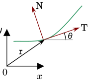
Figure 1: Tangent and Normal to a curve

$$\begin{split}{\bf T}(s)&=\frac{d\widehat{{\bf r}}}{ds}\\ {\bf N}(s)&=\frac{\frac{d{\bf T}}{ds}}{\left|\left|\frac{d{\bf T}}{ds}\right|\right|}\end{split}$$ (2)

The signed curvature $\kappa(s)$ is defined as

$$\kappa(s)=\frac{d\theta}{ds}$$ (3)

where $\theta(s)$ is the tangent angle.

2.2 The discomfort cost functional

From review of comfort studies in road and railway vehicles (Suzuki,, 1998; Jacobson et al.,, 1980; Pepler et al.,, 1980; Förstberg,, 2000; Chakroborty and Das,, 2004; Iwnicki,, 2006), we concluded that for motion comfort, it is necessary to have continuous and bounded acceleration along the tangential and normal directions. It is possible that the actual values of the bounds on the tangential and normal components are different. It is also desirable to keep jerk small and bounded.

We model discomfort as the following cost functional $J$:

$$J=\tau~{}+~{}w_{{\scriptscriptstyle T}}\int_{0}^{\tau}(\dddot{\bf r}\cdot{\bf T})^{2}~{}dt~{}+~{}w_{{\scriptscriptstyle N}}\int_{0}^{\tau}(\dddot{\bf r}\cdot{\bf N})^{2}~{}dt.$$ (4)

Here $\tau$ is the total travel time and ${\bf r}$ is the position of robot at time $t\in[0,\tau]$. $\dddot{\bf r}$ represents the jerk. $\dddot{\bf r}\cdot{\bf T}$ and $\dddot{\bf r}\cdot{\bf N}$ are the tangential and normal components of jerk respectively. The weights ($w_{{\scriptscriptstyle T}}$ and $w_{{\scriptscriptstyle N}})$ are non-negative known real numbers. We separate tangential and normal jerk to allow a choice of different weights ($w_{{\scriptscriptstyle T}}$ and $w_{{\scriptscriptstyle N}}$).

The weights serve two purposes. First, they act as scaling factors for dimensionally different terms. Second, they determine the relative importance of the terms and provide a way to adjust the robot’s performance according to user preferences. For example, for a wheelchair, some users may not tolerate high jerk and prefer traveling slowly while others could tolerate relatively high jerks if they reach their destination quickly. We determine the the typical values of weights using dimensional analysis (see Part I (Gulati et al.,, 2013)).

2.3 Parameterization of the trajectory

The trajectory ${\bf r}$ can be parameterized in various ways. We have found that expressing the trajectory in terms of speed and orientation as functions of a scaled arc-length parameter leads to relatively simple expressions for all the remaining physical quantities (such as accelerations and jerks).

Let $u\in[0,1]$. The trajectory is parameterized by $u$. The starting point is given by $u=0$ and the ending point is given by $u=1$. Let ${\bf r}={\bf r}(u)$ denote the position vector of the robot in the plane. Let $v=v(u)$ be the speed. Both ${\bf r}$ and $v$ are functions of $u$. Let $\lambda$ denote the length of the trajectory. Since only the start and end positions are known, $\lambda$ cannot be specified in advance. It has to be an unknown that will be found by the optimization process.

Let $s\in[0,\lambda]$ be the arc-length parameter. We choose $u$ to be a scaled arc-length parameter where $u=\frac{s}{\lambda}$. The trajectory, ${\bf r}(t),t\in[0,\tau]$ is completely specified by the trajectory length $\lambda$, the speed $v=v(u)$, and the orientation or the tangent angle $\theta=\theta(u)$ to the curve. $\lambda$ is a scalar while speed and orientation are functions of $u$. These are the three unknowns, two functions and one scalar, that will be determined by the optimization process.

With this parameterization, the discomfort cost functional of Equation (4) can be written as

$$J(v,\theta,\lambda)=\int_{0}^{1}\frac{\lambda}{v}du+w_{{\scriptscriptstyle T}}\int_{0}^{1}\frac{v}{\lambda^{3}}(v^{\prime 2}+vv^{\prime\prime}-v^{2}\theta^{\prime 2})^{2}du+w_{{\scriptscriptstyle N}}\int_{0}^{1}\frac{v^{3}}{\lambda^{3}}(3v^{\prime}\theta^{\prime}+v\theta^{\prime\prime})^{2}du.$$ (5)

The first integral ($J_{\tau}$) is the total time, the second integral ($J_{{\scriptscriptstyle T}}$) is total squared tangential jerk, and the third integral ($J_{{\scriptscriptstyle N}}$) is total squared normal jerk.

The discomfort $J$ is now a function of the primary unknown functions $v$, $\theta$, and a scalar $\lambda$, the trajectory length. All references to time $t$ have disappeared. Once the unknowns are found via optimization, we can compute $t$ using the following expression.

$$t=t(u)=\int_{0}^{u}\frac{\lambda}{v(u)}du.$$ (6)

The position vector ${\bf r}(u)$ can be computed via the following integrals.

$${\bf r}(u)={\bf r}(0)+\lambda\left\{\int_{0}^{u}\cos{\theta}(u)\,du,\int_{0}^{u}\sin{\theta}(u)\,du\right\}.$$ (7)

If $\theta(u)$ is known, ${\bf r}(u)$ can be computed from Equation (7). If $v(u)$ and $\lambda$ are known, $t(u)$ can be computed from Equation (6). Using these two, we can determine the function ${\bf r}(t),t\in[0,\tau]$.

The expressions for tangential acceleration $a_{{\scriptscriptstyle T}}$ and normal acceleration $a_{{\scriptscriptstyle N}}$ are

$$a_{{\scriptscriptstyle T}}=\ddot{{\bf r}}\cdot{\bf T}=\frac{vv^{\prime}}{\lambda}$$ (8)

$$a_{{\scriptscriptstyle N}}=\ddot{{\bf r}}\cdot{\bf N}=\frac{v^{2}\theta^{\prime}}{\lambda}.$$ (9)

Here ${\bf N}$ is the direction normal to the tangent (rotated $\frac{\pi}{2}$ anti-clockwise). The signed curvature is given by

$$\kappa(u)=\frac{\theta^{\prime}}{\lambda}$$ (10)

The angular speed $\omega$ is given by

$$\omega(u)=\frac{\theta^{\prime}v}{\lambda}.$$ (11)

2.4 Function spaces for $v$ and $\theta$

We now define the function spaces to which $v$ and $\theta$ can belong so that the discomfort $J$ in Equation (5) is well-defined (finite). We have two distinct cases depending on whether the speed is zero at an end-point on not.

Let $\Omega=[0,1]$ and $H^{2}(\Omega)$ be the Sobolev space of functions on $\Omega$ with square-integrable derivatives of up to order 2. Let $f:\Omega\to\mathbb{R}$. Then

$$f\in H^{2}(\Omega)\stackrel{{\scriptstyle\rm def}}{{\iff}}\int_{\Omega}\left(\frac{d^{j}f}{dx^{j}}\right)^{2}dx<\infty\;\forall\;j=0,1,2.$$ (12)

We can show that if $v,\theta\in H^{2}(\Omega)$, then the integrals of squared tangential and normal jerk are finite. Using the Sobolev embedding theorem (Adams and Fournier,, 2003) it can be shown that if $f\in H^{2}(\Omega)$, then $f^{\prime}\in C^{0}(\Omega)$ and by extension $f\in C^{1}(\Omega)$. Here $C^{j}(\Omega)$ is the space of functions on $\Omega$ whose up to $j^{th}$ derivatives are bounded and continuous. Thus, if $v,\theta\in H^{2}(\Omega)$, then all the lower derivatives are bounded and continuous. Physically this means that quantities like the speed, acceleration, and curvature are bounded and continuous $-$ all desirable properties for comfortable motion (Section 2.2).

We also need that the inverse of $v$ be integrable so that $J_{\tau}$ is finite. Inverse of $v$ is integrable if $v$ is uniformly positive in $[0,1]$. This is trivially true if $v$ is uniformly positive, that is, $v\geq\overline{v}>0$ for some constant positive $\overline{v}$ throughout the interval $[0,1]$. However, $v$ can be zero at one or both end-points because of the imposed conditions (see Section 2.5).

Positive speed on boundary

Consider the case that $v$ is positive on both end-points. We make the justifiable assumption that the trajectory that actually minimizes discomfort will not have a halt in between. Thus, if $v>0$ on end-points, it remains uniformly positive in the interior and the discomfort is finite.

Zero speed on boundary

Consider the case in which $v(0)=0$. The case $v(1)=0$ can be treated in a similar manner. If $v(0)=0$, $\frac{1}{v}$ must not blow up faster than $\frac{1}{u^{p}}$ where $p<1$ to keep $J_{\tau}$ finite. Thus, if zero speed boundary conditions are imposed, we will have to choose $v$ outside $H^{2}(\Omega)$. In such a case, at $u=0$, it is sufficient that $v$ approaches zero as $u^{p}$ where $\frac{3}{5}<p<1$ or $p=\frac{1}{2}$. For the right end point, where $u=1$, replace $u$ with $(1-u)$ in the condition. $v\in H^{2}(\Omega)$ in the interior.

2.5 Boundary conditions

The expression for the cost functional $J$ in Equation (5) shows that the highest derivative order for $v$ and $\theta$ is two. Thus, for the boundary value problem to be well-posed we need two boundary conditions on $v$ and $\theta$ at each end-point $-$ one on the function and one on the first derivative.

We now relate the mathematical requirement on $v$ and $\theta$ boundary values above to expressions of physical quantities. We do this for the starting point only. The ending point relations are analogous.

Positive speed on boundary

First, consider the case when $v>0$ on the starting point. The speed $v$ needs to be specified, which is quite natural. The $u$-derivative of $v$, however, is not tangential acceleration. The tangential acceleration is the $t$-derivative and is given by Equation (8). It is $\frac{vv^{\prime}}{\lambda}$. Here $v$ is known but $\lambda$ is not. Thus specifying tangential acceleration gives us a constraint equation and not directly a value for $v^{\prime}(0)$. This is imposed as an equality constraint. Similarly, fixing a value for $\theta$ on starting point is natural. We “fix” the values of $\theta^{\prime}(0)$ by fixing the signed curvature $\kappa=\frac{\theta^{\prime}}{\lambda}$. As before, this leads to an equality constraint relating $\theta^{\prime}(0)$ and $\lambda$ if $\kappa\neq 0$. Since choosing a meaningful non-zero value of $\kappa$ is difficult, it is natural to impose $\kappa=0$. In this case $\theta^{\prime}(0)=0$ can be imposed easily.

Zero speed on boundary

If $v(0)=0$, then, as seen in Section 2.4, $v(u)$ must behave like $u^{p}$ for $\frac{3}{5}<p<1$ or $p=\frac{1}{2}$ near $u=0$ and $v^{\prime}(u)\sim u^{q}$ for $-\frac{2}{5}<q<0$ or $q=-\frac{1}{2}$ respectively. In this case

$$v^{\prime}(u)\sim u^{-1/3}$$ (13)

is the appropriate strength of the singularity for $v^{\prime}(u)$ at the starting point.

2.6 Obstacle avoidance constraints

We model the “forbidden” region formed by the obstacles as a union of star-shaped domains with boundaries that are closed curves with piecewise continuous second derivative. A set in $\mathbb{R}^{n}$ is called a star-shaped domain if there exists at least one point ${\bf x}_{0}$ in the set such that the line segment connecting ${\bf x}_{0}$ and ${\bf x}$ lies in the set for all ${\bf x}$ in the set. Intuitively this means that there exists at least one point in the set from which all other points are “visible”. We will refer to such a point ${\bf x}_{0}$ as a center of the star-shaped domain.

Let an obstacle be specified by its boundary in polar coordinates that are centered at ${\bf r}_{0}=\{x_{0},y_{0}\}$. Each $\phi\in[0,2\pi)$ gives a point on the boundary using the distance $\rho(\phi)$ from the obstacle origin. The distance function $\rho$ must be periodic with a period $2\pi$. See Figure 2.

Suppose we want a point ${\bf r}=\{x,y\}$ to be outside the obstacle boundary. Define $C({\bf r})$ as

$$C({\bf r})=\left|\left|{\bf r}-{\bf r}_{0}\right|\right|_{2}-\rho(\mbox{arctan2}({\bf r}-{\bf r}_{0}))$$ (14)

where the subscript 2 refers to the Euclidean norm. $C({\bf r})\geq 0\iff$ the point ${\bf r}$ is outside the obstacle.

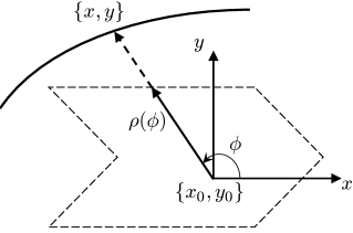
Figure 2: Notation for star-shaped obstacles.

A non-convex star-shaped obstacle is shown with its “center” $\{x_{0},y_{0}\}$ and a distance function $\rho=\rho(\phi)$. The distance function gives a single point on the boundary for $\phi\in[0,2\pi]$. The robot trajectory must lie outside the obstacle.

The constraint function $C({\bf r})$ is piecewise differentiable for all ${\bf r}$ except at a single point ${\bf r}={\bf r}_{0}$. If ${\bf r}={\bf r}_{0}$ by chance, which is easily detectable, we know that the ${\bf r}$ is inside the obstacle and can perturbed to avoid this undefined behavior. Note that $C({\bf r})$ remains bounded inside the obstacle.

3 The infinite-dimensional optimization problem

We now summarize the nonlinear and constrained trajectory optimization problem taking into account all input parameters, all the boundary conditions, and all the constraints. This is the “functional” form of the problem (posed in function spaces). We will present an appropriate discretization procedure valid for all input combinations in the Section 4.

Minimize the discomfort functional $J$, where

$$J(v,\theta,\lambda)=\int_{0}^{1}\frac{\lambda}{v}du+w_{{\scriptscriptstyle T}}\int_{0}^{1}\frac{v}{\lambda^{3}}(v^{\prime 2}+vv^{\prime\prime}-v^{2}\theta^{\prime 2})^{2}du+w_{{\scriptscriptstyle N}}\int_{0}^{1}\frac{v^{3}}{\lambda^{3}}(3v^{\prime}\theta^{\prime}+v\theta^{\prime\prime})^{2}du,$$

given the following boundary conditions for both starting point and ending point

• position (${\bf r}_{0}$, ${\bf r}_{\tau}$),

• orientation ($\theta_{0}$, $\theta_{\tau}$),

• signed curvature ($\kappa_{0}$, $\kappa_{\tau}$),

• speed ($v_{0}\geq 0$, $v_{\tau}\geq 0$),

• tangential acceleration ($a_{{{\scriptscriptstyle T}},0}$, $a_{{{\scriptscriptstyle T}},\tau}$),

and constraints on allowable range of

• speed ($v_{min}=0,v_{max}$),

• tangential acceleration ($a_{{{\scriptscriptstyle T}},min},a_{{{\scriptscriptstyle T}},max}$),

• normal acceleration ($a_{{{\scriptscriptstyle N}},min},a_{{{\scriptscriptstyle N}},max}$),

• angular speed ($\omega_{min},\omega_{max}$),

• curvature, if necessary ($\kappa_{min}=0,\kappa_{max}$),

and

• number of obstacles $N_{obs}$,

• locations of obstacles $\{{\bf c}_{i}\}_{i=1}^{N_{obs}}$

• representation of obstacles that allows computation of $\{\rho_{i}(\phi)\}_{i=1}^{N_{obs}}$, for $\phi\in[0,2\pi)$

and

• an initial guess for $(v(u),\theta(u),\lambda)$, in $u\in[0,1]$,

• weights $w_{{\scriptscriptstyle T}}>0$ and $w_{{\scriptscriptstyle N}}>0$.

The constraint on starting and ending position requires that

$${\bf r}_{\tau}-{\bf r}_{0}=\lambda\left\{\int_{0}^{1}\cos{\theta}\,du,\int_{0}^{1}\sin{\theta}\,du\right\}.$$ (15)

Staying outside all obstacles requires that

$$\left|\left|{\bf r}(u)-{\bf c}_{i}\right|\right|_{2}-\rho_{i}(\mbox{arctan2}({\bf r}(u)-{\bf c}_{i}))\geq 0\;\forall\;i\in 1,\ldots,N_{obs},\mbox{ and}\;\forall\;u\in[0,1]$$

where

$${\bf r}(u)={\bf r}(0)+\lambda\left\{\int_{0}^{u}\cos{\theta}\,du,\int_{0}^{u}\sin{\theta}\,du\right\}.$$

As a post-processing step, we compute time $t$ as a function of $u$ using

$$t=t(u)=\int_{0}^{u}\frac{\lambda}{v(u)}du$$

and convert all quantities ($v,\theta,{\bf r},$ and their derivatives) from $u$ domain to $t$ domain.

4 A finite element discretization of the infinite-dimensional optimization problem

We first discuss the case when there is no singularity in the speed $v$. This is the case when the given boundary speeds are positive. In this case, $v\in H^{2}(\Omega)$ as described in Section 2.4, where $\Omega=[0,1]$. We assume that $\theta\in H^{2}(\Omega)$ always (whether $v$ is singular or not) because it is sufficient for the discomfort to be finite. Thus, to discretize the problem, it is natural to use the basis functions in $C^{1}(\Omega)$, the space of functions that are continuous and have continuous first derivatives. This makes the second derivative of $v$ and $\theta$ discontinuous but its square is still integrable.

4.1 Basis functions

We minimize the discomfort and satisfy all the constraints in a finite dimensional subspace of $C^{1}(\Omega)$. We make the following choice.

$$v^{h}(u) = \sum_{i=1}^{q}\alpha_{i}^{v}\chi_{i}(u)$$ (16)

$$\theta^{h}(u) = \sum_{i=1}^{q}\alpha_{i}^{\theta}\chi_{i}(u)$$ (17)

Here $\chi_{i}(u)\in C^{1}(\Omega)$ are basis functions for this problem. The symbol $h$ traditionally denotes a measure of the “mesh width” to distinguish the approximate solution from the “exact” infinite dimensional solution. The unknown scalar values $\alpha_{i}^{v}$ and $\alpha_{i}^{\theta}$ for $i=1,\ldots,q$ are the degrees of freedom (DOFs) which are to be determined via “solving” the optimization problem of Section 3. For reasonable choices of $\chi_{i}(u)$, as $q$ increases the finite dimensional solution approaches the exact solution.

Usually, one chooses $\chi_{i}(u)\in\Omega$ that are easy and cheap to compute, and have local support. Piecewise polynomial functions that have sufficient differentiability are good candidates. By having local support, we mean the functions are non-zero only over a limited interval and not on whole $\Omega$. This has two main advantages. First, while performing integration to compute $J$, the product of $\chi_{i}$ and $\chi_{j}$ is zero over most of the interval. This leads to $O(n)$ rather than $O(n^{2})$ interactions. Second, the global Hessian matrix is sparse rather than being dense. Typically for 1D problems, the matrix has a small constant band-width.

For our problem, we first divide the interval $[0,1]$ into $n$ equal-size intervals of length $h=\frac{1}{n}$. Each of these intervals is an element. Thus we have $n$ elements and $n+1$ equidistant points or nodes. The collection of elements and nodes is the finite element mesh.

At each node we define two piecewise polynomial functions that are non-zero only on the two elements surrounding the node. This is the standard cubic Hermite basis for problems posed in the $H^{2}$ space in 1D. See Figure 3 for both the functions and their first and second derivatives. The first kind of basis function is 1 on the node with which it is associated and has zero derivative there. The second function is zero on the corresponding node and has unit derivative there. Additionally, both are zero with first derivatives also zero on two surrounding nodes. Thus, in all, we have $2(n+1)$ basis functions and unknown scalars each for $v$ and $\theta$. Because of the above-mentioned properties each basis functions belongs to $C^{1}(\Omega)\subset H^{2}(\Omega)$. Note that the basis functions on the boundary points are slightly different. They are not extended outside the interval. Figure 4 shows 5 basis functions of each kind for $n=4$. As seen, the boundary basis functions are truncated. It would not matter anyway what their values outside the interval are since no integration is performed outside. The other basis functions are translations of each other.

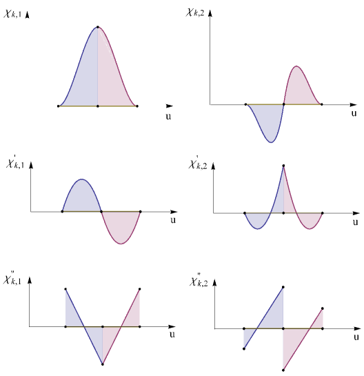
Figure 3: Cubic Hermite basis functions and their first and second derivatives.

Two kinds of basis functions are defined at each node such that each is zero everywhere except on the two elements sharing the node. The first kind, $\chi_{k,1}$ has a value of 1 and a zero derivative at the associated node $k$. Its value and derivatives are zero on both adjacent nodes. The second kind, $\chi_{k,2}$ has a value of zero and a unit derivative at the associated node $k$. Its value and derivatives are zero on both adjacent nodes. Both $\chi_{k,1}$ and $\chi_{k,2}$ are square integrable on $u\in[0,1]$.

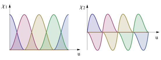
Figure 4: Cubic Hermite basis functions on five consecutive nodes.

The two kinds of basis functions on any node are translations of the respective basis function of Figure 3. The basis functions on a boundary node are truncated.

4.2 Element shape functions

In FEM practice, we define basis functions in terms of “shape functions”. The shape functions are defined only on a single reference element and multiple shape functions placed on neighboring elements are joined to create a single basis function. This requires that shape functions have appropriate values and derivative on reference element boundary so that the basis functions are valid for the problem.

Figure 5 shows the four cubic Hermite shape functions on a single reference element $[0,1]$. The shape functions are

$$\phi_{1}(x) = (x-1)^{2}(1+2x)$$

$$\phi_{2}(x) = (x-1)^{2}x$$

$$\phi_{3}(x) = (3-2x)x^{2}$$

$$\phi_{4}(x) = (x-1)x^{2}$$

For maintaining basis function continuity, each $\phi_{i}$ satisfies $\phi_{i}(0)=\phi_{i}^{\prime}(0)=\phi_{i}(1)=\phi_{i}^{\prime}(1)=0$, except $\phi_{1}(0)=\phi_{2}^{\prime}(0)=\phi_{3}(1)=\phi_{4}^{\prime}(1)=1$.

Figure 5: Cubic Hermite shape functions on a reference element.

Four shape functions are defined on each element. Each is a cubic polynomial on $x=[0,1]$ where $x$ is the local coordinate on the element.

4.3 Singular shape functions at boundary

For the case when either one or both the boundary points have zero speed specified, $v(u)$ is singular at the corresponding boundary with $v^{\prime}(u)$ infinite with singularity $u^{-1/3}$ when acceleration is also zero and $u^{-1/2}$ if acceleration is non-zero. Thus, $v$ as a function does not belong to $H^{2}(\Omega)$. However, $v$ does belong to $H^{2}$ in the interior as shown in Section 2.4.

After a FEM mesh is decided, we take this into account and do not use the above-mentioned regular shape functions for $v$ on the element(s) near the boundary with zero speed. For the interior elements, however, no change is done and the regular shape functions are used.

We now derive the new singular shape functions for the left boundary $(u\in[0,h])$ element and the singular shape functions for the right boundary element can be derived using symmetry.

We need at least two shape functions so that the two shape functions coming from the $[h,2h]$ element can be matched. Denote them by $\psi_{1}^{L}$ and $\psi_{2}^{L}$. The function value and the function derivative both must be matched at $h$. For a reference element shape function, this means $\psi_{1}^{L}(1)=1,{\psi_{1}^{L}}^{\prime}(1)=0,\psi_{2}^{L}(1)=0,{\psi_{2}^{L}}^{\prime}(1)=1$. Both $\psi_{1}^{L}$ and $\psi_{2}^{L}$ must be zero on $u=0$ because the speed is zero there. Thus, the Dirichlet boundary condition is imposed explicitly. Finally, as $x\to 0$, one of the functions must behave as $x^{p}$, for $p=\frac{2}{3}$ or $p=\frac{1}{2}$, to match the singularity in Equation (13). It can be seen that the choice

$$\psi^{L}_{1}(x) = x^{p}+p(1-x)x$$

$$\psi^{L}_{2}(x) = (x-1)x$$

satisfies all these requirements. Figure 6 shows the four shape functions, two for the left element and two for the right element for the case $p=\frac{2}{3}$. Figure 7 shows that $\psi_{1}^{L}$ and $\psi_{1}^{R}$ are singular when approaching the boundary (shown for $p=\frac{2}{3}$ only). The other two functions $\psi_{2}^{L}$ and $\psi_{2}^{R}$ are smooth.

Figure 6: Singular shape functions on boundary elements for zero speed and zero acceleration boundary conditions.

Two singular shape functions are defined on a boundary element. Consider zero speed condition on left element. The first shape function $\psi^{L}_{1}$ has a value of 1 and zero derivative on the right to match the shape function $\phi_{1}$ of Figure 5 on the next element. The second shape function $\psi^{L}_{2}$ has a value of 0 and a unit derivative on the right to match the shape function $\phi_{2}$ of Figure 5 on the next element. Both $\psi^{L}_{1}$ and $\psi^{L}_{2}$ have a value of zero on the left because speed is zero. The singular shape functions for zero speed boundary conditions on right are similarly defined.

Figure 7: First and second derivatives of singular shape functions for zero speed and zero acceleration boundary conditions.

$\psi_{1}^{L}$ and $\psi_{1}^{R}$ tend to infinity as $x^{-\frac{2}{3}}$ as they approach the boundary. $\psi_{2}^{L}$ and $\psi_{2}^{R}$ are smooth.

4.4 The finite-dimensional optimization problem

With the choice of basis functions described above, we can express $v^{h}(u)$ and $\theta^{h}(u)$ as:

$$v^{h}(u) = \sum_{i=1}^{n+1}v_{i}\chi_{i,1}(u)+\sum_{i=1}^{n+1}v^{\prime}_{i}\chi_{i,2}(u)$$ (18)

$$\theta^{h}(u) = \sum_{i=1}^{n+1}\theta_{i}\chi_{i,1}(u)+\sum_{i=1}^{n+1}\theta^{\prime}_{i}\chi_{i,2}(u)$$ (19)

where $v_{i}$, $v^{\prime}_{i}$, $\theta_{i}$, and $\theta^{\prime}_{i}$ for $i=1,\ldots,n$ are the unknown nodal values and $\chi_{i,1}(u)$ and $\chi_{i,2}(u)$ are the two kinds of basis functions described in the previous section.

For optimization, the values of cost, its gradient and Hessian, the values of constraints, and the gradient and Hessian of each constraint are required. For efficiency, it is desirable that cost and constraint Hessians be sparse. We will see later that for the Hessian of obstacle avoidance constraints to be sparse, it is useful to introduce $2N$ additional unknowns in the form of position ${\bf r}_{i}=\left\{x_{i},y_{i}\right\}_{i=1}^{N}$ at $N$ points.

Thus, our objective now is to determine the values of these unknowns and the unknown path length $\lambda$ that minimize the cost functional and satisfy the boundary conditions and constraints described in (Section 3).

Numerical integration for computing the integrals in the cost functional and constraints

We use Gauss quadrature formulas to compute the integrals in the cost functional and constraints. When using $m$ integration points in an interval, the formulas are accurate for polynomials of degree up to $2m-1$. For the regular $C^{1}$ basis functions, which have maximum polynomial degree 3, it is easily seen that the square tangential jerk is a polynomial of degree 23, and the squared normal jerk is a polynomial of degree 17. See Equation (5). These are polynomials in $u$ and not $t$. Hence, 12 Gauss points will give exact integrals up to floating point accuracy. Of course, the integrands being polynomials, the integrals corresponding to $J_{T}$ and $J_{N}$ can be evaluated without using Gauss points (if one is ready to work with complex algebraic expressions). But the other integrals, for $J_{\tau}$ and those relating ${\bf r}$ to $\theta$ (Equation (7)), must be evaluated numerically. Hence, we use 12 Gauss points to evaluate all integrals.

4.5 Imposing constraints

We need to impose multiple equality and inequality constraints while minimizing the cost functional. Some of the equality constraints affect a single DOF each and hence they can be used to eliminate the particular unknown. The others relate multiple DOFs and must be imposed as an equality explicitly. The equality constraints are described below.

• Fix end-point positions (${\bf r}_{0}$, ${\bf r}_{\tau}$) by eliminating the unknowns $x$ and $y$ on the first and last nodes.

• Fix end-point orientations ($\theta_{0}$, $\theta_{\tau}$) by eliminating the unknown $\theta$ on the first and last nodes.

• Relate start and end position ${\bf r}_{\tau}-{\bf r}_{0}=\lambda\left\{\int_{0}^{1}\cos{\theta}\,du,\int_{0}^{1}\sin{\theta}\,du\right\}$ (Equation (15)) by computing the integrals as described in Section 4.6, Equation (20).

• Fix end-point speeds ($v_{0}\geq 0$, $v_{\tau}\geq 0$) by eliminating the unknown $v$ on the first and last nodes.

• If speed on an end-point is positive, tangential acceleration $a_{{\scriptscriptstyle T}}$ must be specified at that end-point. Impose $\frac{vv^{\prime}}{\lambda}=a_{{\scriptscriptstyle T}}$ on that end point. Otherwise, this constraint will be automatically imposed by using singular shape functions.

• Impose specified end-point curvature $\kappa$ by imposing $\theta^{\prime}=\lambda\kappa$ on each end-point.

The inequality constraints that are not related to obstacles avoidance are as follows. We must maintain

• velocity in $[v_{min}=0,v_{max}]$,

• tangential acceleration in $[a_{T,min},a_{T,max}]$,

• normal acceleration in $[a_{N,min},a_{N,max}]$, and

• angular velocity in $[\omega_{min},\omega_{max}]$.

• curvature in $[\kappa_{min}=0,\kappa_{max}]$,

Note that these must be maintained for each $u\in[0,1]$ in the infinite dimensional optimization problem. For the discretized version, we choose the Gauss integration points and impose that these quantities remain in the specified range only on those points. Thus, for a mesh with $n$ elements, each inequality above results in $12n$ constraints (assuming 12 points are used as discussed in Section 4.4). The values of these physical quantities on each Gauss point is a function of the DOFs on element nodes. Thus, these constraints are local. They are not affected when DOFs of non-element nodes change.

There are two important reasons to keep the values within range on Gauss points as opposed to on some other, say, uniform set of points. First, since we use $v$ at the Gauss point to compute the integrals, it is more important that $v$ remain non-negative there to avoid problems of large negative values of $J$. Second, since $v$ and $\theta$ are already computed there it saves extra computation.

4.6 Obstacle avoidance constraints

Staying outside obstacles, if present, requires additional inequality constraints. For this we pick $N$ uniformly separated points in the interval $[0,1]$ and impose the constraint that each of ${\bf r}$ on the $N$ points remain outside each of $N_{obs}$ obstacles. This leads to $N\times N_{obs}$ constraints. In our implementation we make $N=nM+(n+1)$, so that if the distribution is uniform, each element has $M$ such points in the interior and each node is a point too. Two of these $N$ points are the boundary points which must be outside all obstacles for the optimization problem to have a feasible solution. If the robot boundary is not circular and we choose $P$ points on the robot’s boundary, then the number of constraints is $N\times N_{obs}\times P$.

We come back to obstacle related constraint relating a single obstacle and a single point on the trajectory. One could simply relate the position at the point with $\theta(u)$ and $\lambda$ using Equation (7), and use Equation (14) to impose conditions on $\theta(u)$ and $\lambda$. However, because of the structure of Equation (14) and because ${\bf r}(u)$ depends on all $\theta$ DOFs of nodes that are before $u$, the Hessian of this constraint is not sparse. This would lead to efficiency problems when doing iterations in the numerical optimization process. Even computing the dense Hessian would be very costly as $N_{obs}$ and $N$ increase. We must work around this elimination approach of imposing the obstacle related constraints.

To avoid the dense Hessian of obstacle constraint, we make two changes to the simplistic approach. First, we do not use Equation (15) for eliminating ${\bf r}$ but keep ${\bf r}$ as an unknown function. Second, we relate adjacent ${\bf r}$’s via Equation (7) as follows.

$${\bf r}(u_{j})-{\bf r}(u_{j-1})=\lambda\left\{\int_{u_{j-1}}^{u_{j}}\cos{\theta}\,du,\int_{u_{j-1}}^{u_{j}}\sin{\theta}\,du\right\}.$$ (20)

Here $j$ goes from 1 to $N-1$. What this change does is that, as long as adjacent ${\bf r}(u_{j})$ and ${\bf r}(u_{j-1})$ belong to a maximum two adjacent elements, the equation above relates only a small number of local DOFs. Secondly, since each ${\bf r}(u_{j})$ is now a legitimate unknown, it can be used to impose the inequality constraint Equation (14) without $\theta$ being involved.

This new approach does have a price, however. We have increased the number of unknowns and hence increased the size of the gradient vector and Hessian matrix. But this is a small price to pay considering that the sparsity is still maintained, the amount of computation does not grow, and equations are local in nature. We explore the sparsity pattern more in Section 4.7 ahead.

4.7 Element and global gradient and hessian

An important choice in the FEM discretization of any variational problem is the ordering of all the unknowns when forming the global Hessian matrix. A good choice simplifies the assembly process as well as could lead to useful structural sparsity.

We have four kinds of DOFs. For simplicity, we discuss the regular case and where boundary conditions are not yet imposed. The singular case differs in minor details only that does not affect the ordering process. The four kinds are as follows.

• four unknowns each on $n+1$ node $-v,v^{\prime},\theta,\theta^{\prime}$

• $N$ $x$ and $N$ $y$ unknowns

• a scalar unknown $\lambda$

The unknowns are ordered in the same sequence shown above starting from $u=0$ and going to $u=1$.

The ordering chosen above means that each DOF except $\lambda$ interacts with DOFs on two elements. The scaled arc-length parameter, $\lambda$, is global by its nature and interacts with all other DOFs. Hence, the global Hessian matrix is sparse. Some interactions lead to linear equations, so they do not affect the Hessian. This is the case for $x$, $y$, and $\lambda$ interactions in Equation (20).

We now describe the structure of the finite dimensional optimization problem using a small mesh with $n=3$ elements and $N=10$ points for obstacle constraints as shown in Figure 8(a). In FEM, each element provides a small Hessian, typically dense, that relates all the DOFs present in that element. We have eight $v$ and $\theta$ DOFs on each element except for the singular corner elements that have six. Figure 8(b), shows the global connectivity structure of the problem after boundary conditions are imposed on boundary $v,\theta,x,\mbox{ and }y$ DOFs. These are marked $A$ in Figure 8(a). The three element matrices are added to their appropriate positions. The DOFs marked $B$ (for $\theta^{\prime}$) are constrained via equality constraints. The DOFs marked $C$ (for $v^{\prime}$) are constrained via equality constraints if speed is non-zero. Otherwise, it is infinite and is taken care using singular elements. The $x$ and $y$ DOFs do not enter the expression of cost, hence all corresponding rows and columns are empty (zero). The Hessian of obstacles constraints does contain non-zero $2\times 2$ blocks relating $x$ and $y$ of the same point.

(a) A finite element mesh with 3 elements along with $N=10$ $\left\{x,y\right\}$ pairs for obstacle avoidance.

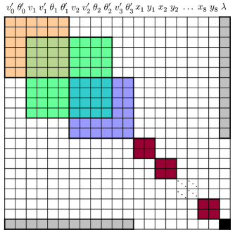
(b) Connectivity structure

Figure 8: Global connectivity structure of the finite dimensional optimization problem.

(a) Some boundary element DOFS and the first and last $\left\{x,y\right\}$ pairs, are set equal to the appropriate boundary conditions and removed from the list of unknowns ($A$). Some boundary element DOFS are related to boundary conditions by equality constraints ($B$). Some are either related to boundary conditions via equality constraints if speed is non-zero, or taken care of by singular elements($C$). (b) All unknowns on a node interact with unknowns on only two neighboring nodes. Each $\left\{x,y\right\}$ pair interacts only with itself. All DOFS on a node interact with $\lambda$.

4.8 Convergence on decreasing mesh size

To analyze the effect of mesh size on convergence, we construct two examples of straight line motion, each with start and end positions as $\left\{0,0\right\}$ and $\left\{10,0\right\}$, and start and end orientations as 0. In the first example, speed at both ends is 0. In the second, speed at both ends is 1. Tangential acceleration at both ends is 0. We vary the number of elements from 2 to 128 in multiples of 2 and each time solve the discomfort minimization problem for one initial guess. As the number of elements increases, the optimum cost found by the optimization process decreases. This is natural because increasing the mesh size means we’re minimizing a function in a superset of degrees of freedom. As the number of elements increases, the relative change in minimum cost decreases. We compare all costs with the cost corresponding to 128 elements. We see that the 32 elements give a cost that within 0.01% of cost for 128 elements (when $v>0$ on end-points). The curve for $v=0$ shows a lower convergence rate and we believe that the reason behind this is using standard Gauss-Legendre quadrature for the singular elements. A more precise procedure would use specially designed quadrature scheme keeping in mind the form of singularity at end-points. We have kept this as part of future work.

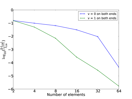
Figure 9: Convergence on decreasing mesh size.

$\log_{10}(\frac{|J-J_{128}|}{J_{128}})$ on $y-$axis against number of elements on $\log_{2}$ scale on $x-$axis. The curve on top is for zero speed boundary conditions on both ends and the curve on bottom is for unit speed boundary conditions on both ends.

5 Initial guess for the optimization problem

We have described a nonlinear constrained optimization problem to find an optimal trajectory that results in a small discomfort. Because of the non-linearity and presence of both inequality and inequality constraints, it is crucial that a suitable initial guess of the trajectory be computed and provided to an optimization algorithm.

Many packages can generate their own “starting points”, but a good initial guess that is within the feasible region can easily reduce the computational effort (measured by number of function and derivative evaluation steps) many times. Not only that, reliably solving a nonlinear constrained optimization problem without a good initial guess can be extremely difficult. Because of these reasons, we invest considerable mathematical and computational effort to generate a good initial guess of the trajectory.

5.1 Overview

As described in Section 2.3, a trajectory can be completely described by its length $\lambda$, orientation $\theta(u)$, and the speed $v(u)$ for $u\in[0,1]$. Our optimization problem is to find the scalar $\lambda$ and the two functions $\theta$ and $v$ that minimize the discomfort. We compute the initial guess of trajectory by computing $\lambda$ and $\theta$ first and then computing $v$ by solving a separate optimization problem. We emphasize that the initial guess computation process must deal with arbitrary inputs and reliably compute the initial guesses.

Before we discuss the initial guess of $\theta$, we must discuss a genuine non-uniqueness issue. It is obvious that there exist infinitely many paths for a given pair of initial and final orientations. There exist at least two different kinds of non-uniqueness. The first kind of non-uniqueness exists because multiple numerical values of an angle correspond to a single “physical” orientation. The second kind of non-uniqueness exists because even for the same numerical values of initial and final angles, one can end up in one of multiple local minima after optimization. We now discuss these in detail.

5.2 Multiplicity of paths

Since the trajectory orientation $\theta$ is an angle, a single $\theta$ value is completely equivalent in physical space to $\theta\pm 2n\pi\;\forall n\in\mathbb{N}$. However, consider a trajectory that starts with a given angle $\theta_{0}$, and stops at orientation $\theta_{\tau}$ (where $\tau$ denotes final time). Such a trajectory will be different than a trajectory that starts off with the same orientation but stops at $\theta_{\tau}\pm 2n\pi$. This is because $\theta$ is continuous and cannot jump to a different value in between. Of course, the boundary condition will still be satisfied. Thus, even though the original trajectory optimization problem is specified using a single stopping orientation, we must consider multiple stopping orientations, differing by $2\pi$, when computing the initial guess as well as solving the original discomfort minimization problem. We have called this a “parity” problem. Note that the same logic of parity applies to the starting orientation, but what matters is the difference and we have chosen to vary only the ending orientation by choosing different values of $n$.

Figure 10(b) shows a few examples of this parity. It shows four paths corresponding to different $n$ each sharing a common starting angle, but reach the destination at $\{-3\pi,-\pi,\pi,3\pi\}$. Of course, we could create more paths by increasing the $2\pi$ difference but doing so makes the paths more convoluted and self-intersecting in general. This is because when $n$ is too large in magnitude, $\theta(u)$ has to vary rapidly at least around some $u$ values in $[0,1]$ to satisfy the larger difference in boundary conditions. For optimization purposes, we assume that the starting and ending orientations are given between $[0,2\pi)$ and we choose just three end-point orientations that give the least difference $\left|\theta_{\tau}-\theta_{0}\right|$.

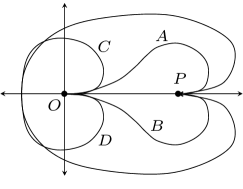
(a) Four paths

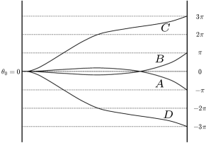
(b) Four $\theta$ curves

Figure 10: Four paths with different parity

The paths $A,B,C,$ and $D$ start from $O$ and reach $P$ at identical physical angles but, looked as $\theta$ curves, their ending angles differ by integer multiples of $2\pi$.

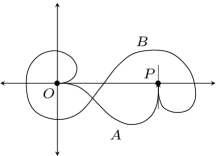
(a) Two paths

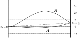
(b) Two $\theta$ curves

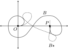
(c) Deformed path

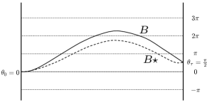
(d) Deformed $\theta$ curve

Figure 11: (Two local minima for same boundary conditions

(a)(b) The paths $A$ and $B$ are different but both minimize discomfort compared to neighboring paths. (c)(d) $B_{*}$ is obtained by a continuous deformation of $B$. The $\theta$ curves of $B$ and $B*$ are similar. The corresponding paths show that $B*$ contains two self intersections and is topologically different from $A$ that does not contain self intersections.

Apart from the multiplicity of $\theta$ curves due to parity, the optimization problem discussed Section 5.3 to compute $\theta$ as well as the full discomfort minimization problem can lead to multiple solutions even when parity remains unchanged. This occurs due to the non-linearity of constraints in Equation (15). Figure 11(d)(a) and (b) shows two such paths $A$ and $B$ that start and end at the same numerical orientation but are qualitatively different. We do observe such multiple minima in practice. If we observe $B$ more carefully, it is seen that it can be continuously deformed into $B*$ shown in Figure 11(d)(c) and (d). This figure clearly shows that the reason $B$ is qualitatively different from $A$ is because of two self-intersections $-$ first in anti-clockwise direction and second in clockwise direction. Both “loops” cancel each others’ changes in orientation. We suspect that this topological difference is the cause of multiple local minima.

Of course, this argument can be carried further and one can introduce an equal number of clockwise and anti-clockwise loops in arbitrary order and the final orientation will remain unchanged. Thus, we believe that there can be infinitely many local minima. Obviously, doing so would increase the discomfort in general and such a path will not be desirable. We try to avoid this problem by setting bounds on maximum and minimum $\theta$ when we compute the initial guess of $\theta$. However, it is important to not ignore multiple minima if they are found within these bounds. If obstacles are present so that $A$ is infeasible, $B$ might be chosen even though it is longer and has more turns.

Thus, because of these two kinds of multiplicities, we use more than one initial guess when minimizing the discomfort and choose the one that has the minimum discomfort and satisfies the constraints. We discuss the details in the following section.

5.3 Initial guess of path

We compute initial guesses for $\lambda$ and $\theta(u)$ using two different methods. The first method computes a $\theta(u)$ such that the trajectory has a piecewise constant curvature. This is a computationally inexpensive method and does not satisfy many of the constraints exactly. The output of this method can be used to solve the full discomfort minimization problem.

The second method computes a $\theta(u)$ and $\lambda$ by solving an auxiliary (but simpler) nonlinear constrained optimization problem. Of course, now we need an initial guess for this new optimization problem! The output of the “constant curvature” method mentioned above is used as the initial guess. Unlike the first method, the output of this second method leads to trajectories that have continuous and differentiable curvature and also satisfy boundary conditions and maximum curvature constraint exactly.

Piecewise constant curvature path

In the full discomfort minimization problem, the orientation $\theta(u)$ has to satisfy the boundary conditions and Equation (15). In total, there are four constraints $-$ two linear (those due to boundary conditions) and two non-linear (those of Equation (15)).

For computing initial guess of $\theta$, we modify the inputs of the full optimization problem using a rotation such that initial and final position have the same $y$ coordinate value. The initial and final orientations are also modified appropriately. Once we find an initial guess for the transformed input, it can be easily transformed back to the original configuration by the inverse rotation. This is done to allow efficient storage of precomputed $\theta$ guesses for various end-point conditions.

Thus, the inputs to the initial guess generation problem are the initial and final positions, $x_{0}$ and $x_{\tau}$, and orientations, $\theta_{0}$ and $\theta_{\tau}$, in the rotated frame. The output will be a path length $\lambda$ and a function $\theta(u)$.

We begin by choosing the value of path length $\lambda$ as max$(R,2*\Delta L)$, where $R$ is the minimum turning radius of the robot and $\Delta L=\left|\left|{\bf r}_{\tau}-{\bf r}_{0}\right|\right|$. Using this maximum takes care of the case when initial and final positions are very close to each other. In such a case, the path length is decided by the minimum turning radius constraint.

Ideally, an initial guess of $\theta(u)$ should obey the following constraints so that the constraints of the full optimization problem are satisfied:

$$\begin{split}\theta(0)&=\theta_{0},\\ \theta(1)&=\theta_{\tau},\end{split}$$ (21)

and transformed Equation (15)

$$\begin{split}\lambda\int_{0}^{1}\cos{\theta}\,du&=x_{\tau}-x_{0},\\ \lambda\int_{0}^{1}\sin{\theta}\,du&=0,\end{split}$$ (22)

Consider a piecewise linear function that looks like the solid curves in Figure 12(d)(b).

(a) Cost from Equation (24)

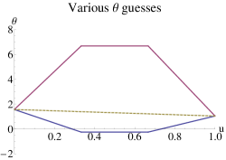
(b) Two constant curvature optimizers

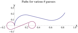
(c) Paths corresponding to (b)

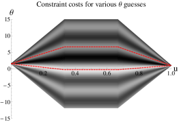
(d) Multiple local minima

Figure 12: Piecewise constant curvature initial guesses

(a) Multiple local minima in graph of $J_{cc}$ of Equation (24). Two minima closest to the maxima are highlighted. (b) Piecewise constant curvature paths (not dashed) corresponding to highlighted minima in (a). (c) Paths corresponding to the $\theta$ curves in (b). Both start at $\frac{\pi}{2}$ and end at $\frac{\pi}{3}$. (d) Lighter shade represents minima and darker shade represents maxima. The two optimizing paths of (b) are shown.

Essentially, each such curve is defined on $[0,1]$, is continuous, and is made of three line segments in $[0,\frac{1}{3}]$, $[\frac{1}{3},\frac{2}{3}]$, and $[\frac{2}{3},1]$. The middle line segment has zero derivative. The values at 0 and 1 are known and the only variable is the function value on the middle segment. Equivalently, one can use the slope of first line segment as the variable. Let this slope be denoted by $\theta^{\prime}_{1}$. Then, we define $\theta(u)$ as

$$\theta(u)=\left\{\begin{array}[]{rll}\theta_{0}+\theta^{\prime}_{1}u&\mbox{if}&0\leq u<\frac{1}{3};\\ \theta_{0}+\frac{1}{3}\theta^{\prime}_{1}&\mbox{if}&\frac{1}{3}\leq u<\frac{2}{3};\\ \theta_{0}+\frac{1}{3}\theta^{\prime}_{1}-3(\theta_{0}-\theta_{1}+\frac{1}{3}\theta^{\prime}_{1})(u-\frac{2}{3})&\mbox{if}&\frac{2}{3}\leq u\leq 1.\end{array}\right.$$ (23)

If we use such a curve for $\theta(u)$, it will result in a circular arc, a tangent line segment, and another circular arc tangential to the middle segment, in that order. This, in turn, implies that the resulting path will have a piecewise constant curvature.

To determine $\theta(u)$, we need to determine the value of the unknown slope $\theta^{\prime}_{1}$. Since only one value cannot satisfy two constraints of Equation (22), we minimize

$$J_{cc}(\theta^{\prime}_{1})=\left(\int_{0}^{1}\cos{\theta}\,du-1\right)^{2}+\left(\int_{0}^{1}\sin{\theta}\,du\right)^{2}$$ (24)

to find $\theta^{\prime}_{1}$. Figure 12(d)(a) shows the plot of $J_{cc}$ as a function of $\theta^{\prime}_{1}$. Depending on the boundary conditions, the shape of $J_{cc}$ changes but qualitatively it has the behavior as shown $-$ oscillatory with a maximum not too far from zero. We find this maximum using a table lookup and the neighboring two minima to compute the initial guess. Figure 12(d)(c) shows two paths using this method where $\theta_{0}=\frac{\pi}{2}$ and $\theta_{\tau}=\frac{\pi}{3}$. The path length is 1. As seen, the curve end-point is not too far from $x-$axis, and the curve satisfies the boundary condition on $\theta$. Figure 12(d)(d) shows the cost $J_{cc}$ for various constant curvature paths. The lighter shade corresponds to the minima.

Optimization approach for initial guess of path

In this second method to compute the initial guess of the path, we minimize

$$J(\theta,\lambda)=\lambda+w\int_{0}^{1}\theta^{\prime\prime 2}du$$ (25)

where $w:=\max(\Delta L,R)$, and $\theta$ must satisfy the boundary conditions, the two equality constraints of Equation (15), and the curvature constraint

$$\left|\theta^{\prime}(u)\right|\leq\lambda\kappa_{\max}\;\forall u\in[0,1].$$

We do not impose the obstacle related constraints in this problem. This problem is related to the concept of “Minimum Variation Curves” Moreton, (1993) which have been proposed for curve shape design. We add the curve length $\lambda$ so that in the presence of multiplicities, discussed in Section 5.2 earlier, the curves with smaller lengths are preferred. This optimization problem is discretized using $C^{1}$ finite elements as described in Section 4.2, and the initial guess is the piecewise constant curvature function from Section 5.3.

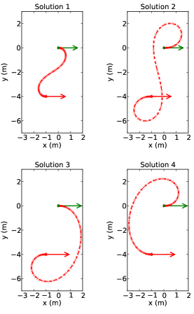
Figure 13: Four initial guess of path.

Problem input is as follows: initial position = $\left\{0,0\right\}$, orientation = 0, speed = 0, tangential acceleration = 0; final position = $\left\{-1,-4\right\}$, orientation = 0, speed = 0, tangential acceleration = 0. The four initial guesses of path are computed using the method described in Section 5.3 so that final orientation in (a),(b),(c) and (d) is 0, 0, $-2\pi$ and $2\pi$ respectively. All quantities have appropriate units in terms of meters and seconds. Initial and final positions are shown by markers and orientations are indicated by arrows. While the path is parameterized by $u$, for ease of visualization, we show markers at equal intervals of time. Thus distance between markers is inversely proportional to speed.

5.4 Initial guess of speed

Computing the initial guess of $v$ is relatively simpler. We solve a convex quadratic optimization problem with linear inequality box constraints to compute the initial guess. Because of convexity of the functional and the convex shape of the feasible region, this problem has a unique solution and an initial guess is not necessary to solve it. Any good quality optimization package can find the solution without an initial guess. Of course, because of the simplicity of box constraints, we can and do provide a feasible initial guess for this auxiliary problem.

First consider the case when both end-points have non-zero speed. We minimize

$$J(v)=\int_{0}^{1}v^{\prime\prime 2}du$$ (26)

subject to boundary constraints $v(0)=v_{0}>0$, $v(1)=v_{1}>0$, $v^{\prime}(0)=\frac{a_{0}\lambda}{v_{0}}$, $v^{\prime}(1)=\frac{a_{1}\lambda}{v_{1}}$ and inequality constraints $v_{\min}(u)\leq v(u)\leq v_{\max}(u)$ and $A_{\min}(u)\leq v^{\prime}(u)\leq A_{\max}(u)$. The expressions for $v^{\prime}(0)$ and $v^{\prime}(1)$ come from the relation in Equation (8). The length $\lambda$ is computed when the initial guess for $\theta$ is computed. Here we choose $v_{\min}(u)=\min(v_{0},v_{1})/2$ and $v_{\max}(u)$ is a constant that comes from the hardware limits. The function $A_{\min}(u)$ is chosen to be the constant $10a_{\min}\lambda/\min(v_{0},v_{1})$ where $a_{\min}$ is the minimum allowed physical acceleration. $A_{\max}(u)$ is chosen similarly using $a_{\max}$.

This optimization problem is discretized using $C^{1}$ finite elements as described in Section 4.2 and leads to a convex programming problem that is easily solved. Of course, this method does not take care of cases in which one or both points have zero speed boundary conditions.

If both end-points have zero speeds, the function

$$v(u)=v_{\max}\left(4u(1-u)\right)^{2/3}$$ (27)

satisfies the boundary conditions and singularities and has a maximum value of $v_{\max}$. This case does not require any optimization.

If only one of the end-points has a zero speed boundary condition, we split the initial guess for $v$ into a sum of two functions. The first one takes care of the singularity and the second takes care of the non-zero speed boundary condition on the other end-point. We now maintain only the $v_{\max}$ constraint because $v^{\prime}(u)$ is unbounded and $v_{\min}=0$ naturally. If the right end-point has zero speed, we choose

$$v(u)=v_{\mbox{singular}}(u)+v_{\mbox{non-singular}}(u)$$

where

$$v_{\mbox{singular}}(u)=\frac{16}{9}2^{1/3}v_{\max}u^{2}(1-u)^{2/3}.$$

This function has the correct singularity behavior and its maximum value is $v_{\max}/2$. The non-singular part is computed via optimization so that the sum is always less than $v_{\max}$. For the other case, when left end-point has zero speed, the singular part (using symmetry) is

$$\frac{16}{9}2^{1/3}v_{\max}(1-u)^{2}u^{2/3}.$$

Figure 14 shows these different cases. All the imposed bounds are maintained and the initial guesses of $v$ are smooth curves for all kinds of boundary conditions. For non-zero boundary speed, the values are 1 on the starting point and 2 on the ending point. Maximum speed is 3. Where imposed, $A_{\min}=-50$ and $A_{\max}=50$.

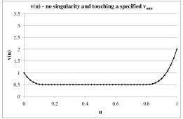
(a) $v_{\min}=0.5$ is active

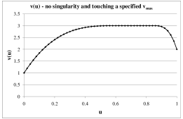
(b) $v_{\max}=3$ is active

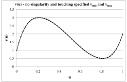
(c) Both $v_{\min}$ and $v_{\max}$ active

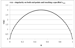
(d) Both ends singular and $v(u)=v_{\max}\left(4u(1-u)\right)^{2/3}$

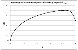
(e) $v_{\max}=3$ is active, singular start

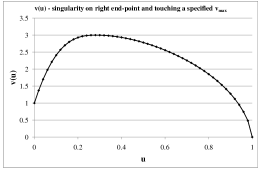
(f) $v_{\max}=3$ is active, singular end

Figure 14: Initial guesses for speed

5.5 Implementation details

We have implemented our code in C++. We use Ipopt, a robust large-scale nonlinear constrained optimization library (Wächter and Biegler,, 2006), also written in C++, to solve the optimization problem to compute the initial guess of path (Section 5.3) and speed (Section 5.4). We explicitly compute gradient and Hessian problem in our code instead of letting Ipopt compute these using finite difference. This leads to greater robustness and faster convergence. We set the Ipopt parameter for relative tolerance as $10^{-8}$ and the maximum number of iterations to $100$.

5.6 Computational time for initial guess

To evaluate the reliability of our method, we constructed a set of $7500$ problems with different boundary conditions and solved the full constrained optimization problem corresponding to each of the 4 initial guesses for each problem. We present an analysis of the reliability and run-time for the initial guesses for this problem set.

We generate the problem set as follows. Fix the initial position as $\left\{0,0\right\}$ and orientation as 0. Choose final position at different distances along radial lines from the origin. Choose 10 radial lines that start from 0 degrees and go up to 180 degrees in equal increments. The distance on the radial line is chosen from the set $\left\{1,2,4,8,16\right\}$. The angle of the radial line and the distance on the line determines the final position. Choose 30 final orientations starting from 0 up to 360 degrees (360 degrees not included) in equal increments. The speed, $v$, and tangential acceleration, $a_{{\scriptscriptstyle T}}$, at both ends are varied by choosing $\left\{v,a_{{\scriptscriptstyle T}}\right\}$ pairs from the set $\left\{\left\{0,0\right\},\left\{1,-0.1\right\},\left\{1,0\right\},\left\{1,0.1\right\},\left\{3,0\right\}\right\}$. Thus we have 10 radial lines, 5 distances on each radial line, 30 orientations, 5 $\left\{v,a_{{\scriptscriptstyle T}}\right\}$ pairs, resulting in $10\times 5\times 30\times 5=7500$ cases. Each problem has $189$ degrees of freedom.

All the problems were solved on a computer with an Intel Core i7 CPU running at 2.67 GHz, 4 GB RAM, and 4 MB L-2 cache size. Histograms of run-time for computing initial guess of speed and initial guess of path are shown in Figures 16 and  16 respectively. Histograms for all four initial guesses and all four discomfort minimization problems are shown. In all these histograms, we have removed 1% or less of cases that lie outside the range of the axis shown for better visualization. All histograms show both successful and unsuccessful cases.

For all 7500 problems, at least one initial guess was successfully computed. From Figure 16 we see that than 99% or more of initial guesses of path are computed in less than 0.2 s. From Figure 16 we see that 99% or more of initial guesses of speed are computed in less than 0.12 s.

These initial guesses were used to solve the full nonlinear optimization problem. Results for the full problem are presented in Part I. Here is a summary. Out of a set of $7500$ examples with varying boundary conditions, and all dynamic constraints imposed, 3.6 solution paths, on average, were found per example. At least one solution was found for all of the problems and four solutions were found for roughly 60% of the problems. The time taken to compute the solution to the discomfort minimization problem was less than 10 seconds for all the cases, 99% of all problems were solved in less than 4 seconds, and roughly 90% were solved in less than 100 iterations.

(a) 99% solved within 0.2 s.

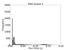
(b) 99% solved within 0.2 s.

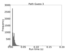
(c) 100% solved within 0.2 s.

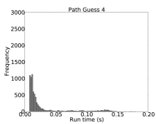
(d) 100% solved within 0.2 s.

Figure 15: Histogram of time taken to compute initial guess of path. Total 7500 cases.

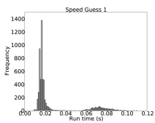
(a) 99% solved within 0.12 s.

(b) 99% solved within 0.12 s.

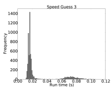
(c) 99% solved within 0.12 s.

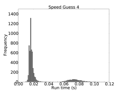
(d) 99% solved within 0.12 s.

Figure 16: Histogram of time taken to compute initial guess of speed. Total 7500 cases.

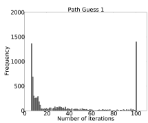
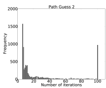
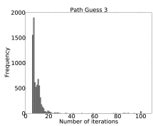
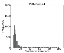
Figure 17: Histogram of number of iterations to compute initial guess of path.

6 Acknowledgements

This work has taken place in the Intelligent Robotics Lab at the Artificial Intelligence Laboratory, The University of Texas at Austin. Research of the Intelligent Robotics lab was supported in part by grants from the National Science Foundation (IIS-0413257, IIS-0713150, and IIS-0750011), the National Institutes of Health (EY016089), and from the Texas Advanced Research Program (3658-0170-2007).

References

- Adams and Fournier, (2003) Adams, R. A. and Fournier, J. F. (2003). Sobolev spaces. Elsevier.
- Chakroborty and Das, (2004) Chakroborty, P. and Das, A. (2004). Principles of Transportation Engineering. PHI Learning Pvt. Ltd.
- Choset et al., (2005) Choset, H., Lynch, K. M., Hutchinson, S., Kantor, G., Burgard, W., Kavraki, L. E., and Thrun, S. (2005). Principles of Robot Motion: Theory, Algorithms, and Implementations. MIT Press.
- Fehr et al., (2000) Fehr, L., Langbein, W. E., and Skaar, S. B. (2000). Adequacy of power wheelchair control interfaces for persons with severe disabilities: A clinical survey. Journal of Rehabilitation Research and Development, 37(3):353–ֳ60.
- Förstberg, (2000) Förstberg, J. (2000). Ride comfort and motion sickness in tilting trains: Human responses to motion environments in train experiment and simulator experiments. PhD thesis, KTH Royal Institute of Technology.
- Gulati, (2011) Gulati, S. (2011). A framework for characterization and planning of safe, comfortable, and customizable motion of assistive mobile robots. In Ph.D. Thesis.
- Gulati et al., (2013) Gulati, S., Jhurani, C., and Kuipers, B. (2013). A nonlinear constrained optimization framework for comfortable and customizable motion planning of nonholonomic mobile robots – part i. Submitted to The International Journal of Robotics Research.
- Hughes, (2000) Hughes, T. J. (2000). The Finite Element Method: Linear Static and Dynamic Finite Element Analysis. Dover Publications.
- Iwnicki, (2006) Iwnicki, S. (2006). Handbook of Railway Vehicle Dynamics. CRC Press.
- Jacobson et al., (1980) Jacobson, I. D., Richards, L. G., and Kuhlthau, A. R. (1980). Models of human comfort in vehicle environments. Human factors in transport research, 20:24–32.
- Latombe, (1991) Latombe, J.-C. (1991). Robot Motion Planning. Kluwer Academic Press.
- LaValle, (2006) LaValle, S. M. (2006). Planning Algorithms. Cambridge University Press.
- (13) LaValle, S. M. (2011a). Motion planning: The essentials. IEEE Robotics and Automation Society Magazine, 18(1):79–89.
- (14) LaValle, S. M. (2011b). Motion planning: Wild frontiers. IEEE Robotics and Automation Society Magazine, 18(2):108–118.
- Moreton, (1993) Moreton, H. P. (1993). Minimum Curvature Variation Curves, Networks, and Surfaces for Fair Free-Form Shape Design. PhD thesis, EECS Department, University of California, Berkeley.
- Pepler et al., (1980) Pepler, R. D., Sussman, E. D., and Richards, L. G. (1980). Passenger comfort in ground vehicles. Human factors in transport research, 20:76–84.
- Silberg et al., (2012) Silberg, G., Wallace, R., Matuszak, G., Plessers, J., Brower, C., and Subramanian, D. (2012). Self-driving cars: The next revolution. Technical report, KPMG Center for Automotive Research.
- Simpson et al., (2008) Simpson, R. C., LoPresti, E. F., and Cooper, R. A. (2008). How many people would benefit from a smart wheelchair? Journal of Rehabilitation Research and Development, 45(1):53–72.
- Suzuki, (1998) Suzuki, H. (1998). Research trends on riding comfort evaluation in japan. Proceedings of the Institution of Mechanical Engineers – Part F – Journal of Rail and Rapid Transit, 212(1):61–72.
- Wächter and Biegler, (2006) Wächter, A. and Biegler, L. T. (2006). On the implementation of a primal-dual interior point filter line search algorithm for large-scale nonlinear programming. Mathematical Programming, 106(1):25–57.