Estimating Photometric Redshifts of Quasars via K-nearest Neighbor Approach Based on Large Survey Databases

Abstract

We apply one of lazy learning methods named $k$-nearest neighbor algorithm ($k$NN) to estimate the photometric redshifts of quasars, based on various datasets from the Sloan Digital Sky Survey (SDSS), UKIRT Infrared Deep Sky Survey (UKIDSS) and Wide-field Infrared Survey Explorer (WISE) (the SDSS sample, the SDSS-UKIDSS sample, the SDSS-WISE sample and the SDSS-UKIDSS-WISE sample). The influence of the $k$ value and different input patterns on the performance of $k$NN is discussed. $k$NN arrives at the best performance when $k$ is different with a special input pattern for a special dataset. The best result belongs to the SDSS-UKIDSS-WISE sample. The experimental results show that generally the more information from more bands, the better performance of photometric redshift estimation with $k$NN. The results also demonstrate that $k$NN using multiband data can effectively solve the catastrophic failure of photometric redshift estimation, which is met by many machine learning methods. By comparing the performance of various methods for photometric redshift estimation of quasars, $k$NN based on KD-Tree shows its superiority with the best accuracy for our case.

1 Introduction

Astronomy steps into an era of abundant photometric data with the development of CCD and other modern technologies. Several wide-field surveys with large ground- and space-based telescopes will produce over a hundred million photometric data which are larger than spectroscopic data by two or three orders of magnitude. The most representative survey should be the Sloan Digital Sky Survey (SDSS, York et al. 2000), which greatly promotes the development of modern astronomy and improves the methods of analyzing massive astronomical data. Many advanced data mining and machine learning algorithms (See reviews written by Zhang et al. 2008, Borne 2009 and Ball & Brunner 2010) have been successfully applied to deal with problems caused by massive astronomical data sets, such as galaxy classification, quasar candidate selection, photometric redshift estimation and so on. In the next decade, the ongoing and planned multiband photometric surveys, for instance, the above mentioned SDSS, the United Kingdom Infrared Telescope (UKIRT; Lawrence et al. 2007), the Large Synoptic Survey Telescope (LSST; Tyson 2002), the Panoramic Survey Telescope and Rapid Response System (Pan-STARRS; Kaiser et al. 2002) and so on, will bring many more challenges for astronomers. This situation will make the technologies of data mining and machine learning become more popular among the astronomical community.

Photometric redshifts are a very important and powerful statistical tool for providing distances of celestial objects to study the evolutionary properties of galaxies and cosmology. Photometric redshifts are those derived from only images or photometry. So far the techniques of photometric redshifts have been in a bloom while deep multicolor photometric surveys have been carried out, with lots of objects inaccessible to spectroscopic observations or too time consuming with the available instruments. The techniques are divided into two types: empirical methods and the template-fitting approach. Empirical methods use a subsample of the photometric data with spectroscopic redshifts as a training set for the redshift estimators, this subsample describes the redshift distribution in magnitude and color space empirically and is utilized to construct regressors to predict photometric redshifts. A lot of machine learning techniques show good performance on the problem of determining photometric redshifts of galaxies or quasars. Artificial Neural Networks (ANN) have been used by astronomers (Firth et al. 2003; Collister & Lahav 2004; Blake et al. 2007; Oyaizu et al. 2008; Y$\grave{e}$che et al. 2010; Zhang et al. 2009) for determining photometric redshifts. In recent years, many other algorithms for photometric redshifts have entered into our sight. Way et al. (2009) demonstrated that Gaussian Process Regression (GPR) can be a competitive approach to ANN and other least-squares fitting methods. Geach (2011) presented an application of the Self-Organized Map (SOM) for visualizing, exploring and mining the catalogues of large astronomical surveys. Weak Gated Experts (WGE) which allows to derive photometric redshifts through a combination of data mining techniques was presented by Laurion et al. (2011). Ball et al. (2007; 2008) discussed how to apply a nearest neighbor algorithm to predict photometric redshifts. Polsterer et al. (2013) applied $k$-nearest neighbor approach to estimate photometric redshifts of quasars and preselect high-redshift quasar candidates. Wadadekar (2005) employed Support Vector Machines (SVMs) to predict photometric redshifts of galaxies. However, SVMs is not a good choice for estimating photometric redshifts (Wang et al. 2008; Peng et al. 2010a). Template methods use either libraries of observed spectra exterior to the survey or model spectral energy distributions (SEDs). Since these are full spectra, the templates can be shifted to any redshift and then convolved with the transmission curves of the filters used in the photometric survey to create the template set for the redshift estimators. There are many works on the SED fitting technique or template fitting technique, for example, Bolzonella et al. 2000, Budav$\acute{a}$ri et al. (2000, 2001), Babbedge et al. (2004), Rowan-Robinson et al. (2008), Wolf et al. (2008, 2009), Wu et al. (2010), Ilbert et al. (2009, 2011), Salvato et al. (2009, 2011). In addition, some researches focus on comparison of methods for photometric redshift estimation (Hildebrandt et al. 2010; Abdalla et al. 2011; Oyaizu et al. 2008; Wang et al. 2008).

In this work we attempt to use $k$-nearest neighbor ($k$NN) algorithm which is a simple algorithm and easy to be understood by astronomers to estimate photometric redshifts of quasars. This method will be used to determine the photometric redshifts of quasars which are much more challenging than those of galaxies because there is a catastrophic failure in estimating photometric redshifts of quasars when the spectroscopic redshift is less than 3. All wide-field quasar photometric redshift results suffer this problem (e.g. Weinstein et al. 2004; Richards et al. 2001; Wu et al. 2004). In the following we apply $k$-nearest neighbor with multiband data based on the SDSS (the Sloan Digital Sky Survey), UKIDSS (the UKIRT Infrared Deep Sky Survey) and WISE (the Wide-field Infrared Survey Explorer) databases to solve this problem.

This paper is organized as follows. Section 2 describes the characteristics of data used in this experiment in detail. In Section 3.1, we present the principle of $k$NN, and discuss some detail of it. Section 3.2 demonstrates the performance of $k$NN using multiband datasets for estimating photometric redshifts of quasars. In Section 4, we give the conclusion and what should be improved in the future work.

2 Data

There are three data sets used in this work. The first set is generated from the Sloan Digital Sky Survey (SDSS; York et al. 2000) which could be one of the most ambitious and influential surveys in the history of astronomy. Since we focus on the photometric redshift estimation of quasars, we use the samples of the Quasar Catalogue V (Schneider et al. 2010) with highly reliable redshifts as our basic data set. Based upon the SDSS DR7 (Abazajian et al. 2009), quasar Catalogue V contains 105,783 spectroscopically confirmed quasars and represents the conclusion of the SDSS-I and SDSS-II quasar survey. We cross-identify all quasars in this table with the UKIRT (UK Infrared Telescope) Infrared Deep Sky Survey (UKIDSS) (Warren et al. 2000; Lawrence et al. 2007) data release eight (DR8) and the whole data release of the NASA’s Wide-field Infrared Survey Explorer (WISE; Wright et al. 2010), respectively.

For the cross-matching of Quasar Catalogue V with UKIDSS DR7, we adopt the closest counterparts within 3 arcsec radius between the positions in the two catalogs. In order to avoid the area of lower Galactic latitudes which is crowed with many stellar objects, we only adopt the data in the UKIDSS Large Area Survey (LAS) (Wu et al. 2010). In the left panel of Figure 1, the distribution of the positional offset between SDSS and UKIDSS is shown by a dotted line. It clearly shows that almost all (99.68%) of the closest counterparts are within 0.5 arcsec of the SDSS positions. We then cross-match Quasar Catalogue V with WISE pre within 6 arcsec radius given that the angular resolution of WISE is 6.1 arcsec, 6.4 arcsec, 6.5 arcsec and 12.0 arcsec in the four bands (W1, W2, W3, W4), respectively. In the left panel of Figure 1, the positional offset distribution of the cross-match result of the two data sets is indicated by a solid line and it is found that 86.74% of the cross-match sources have offsets smaller than 1 arcsec and 95.57% of them have offsets smaller than 2 arcsec.

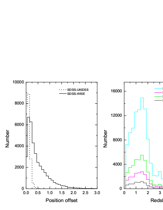
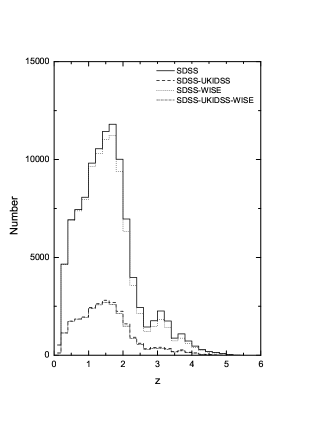
Figure 1: Left: The positional offset distribution of SDSS-UKIDSS and SDSS-WISE. Right: The quasar redshift distribution of SDSS (solid line), SDSS-UKIDSS (dash line), SDSS-WISE (dot line) and SDSS-UKIDSS-WISE samples(dash dot line).

As a result, in order to improve the probability and reliability of cross-identification, the cross-match radius between SDSS and UKIDSS DR8 is taken 0.5 arcsec, the radius between SDSS and WISE is set 2 arcsec. Thus the number of quasars for the SDSS-UKIDSS and SDSS-WISE samples is 25184 and 100208, respectively. For the SDSS-UKIDSS and SDSS-WISE samples obtained by the front steps, the same SDSS ID of sources are collected as the SDSS-UKIDSS-WISE sample. The number of this sample is 24089. Consequently, the number of SDSS-UKIDSS-WISE quasars is smaller than the other two quasar samples.

In the right panel of Figure 1, we plot the redshift histogram of quasars for the four samples of SDSS, SDSS-UKIDSS, SDSS-WISE and SDSS-UKIDSS-WISE. The distributions of the SDSS and SDSS-WISE samples are very similar, those of the SDSS-UKIDSS and SDSS-UKIDSS-WISE samples are just alike. Considering Galactic extinction, magnitudes from SDSS are corrected by the dust reddening map of Schlegel et al. (1998). Since UKIDSS and WISE surveys both use the Vega Magnitude system, we decide to convert dereddened SDSS AB magnitudes to Vega magnitudes using the rules described by Hewett et al. (2006). In the following experiments, $u,g,r,i,z$ all points to dereddened SDSS $u,g,r,i,z$ in Vega system, respectively.

3 METHOD

3.1 $k$NN

In pattern recognition, the $k$-nearest neighbor algorithm ($k$NN) is a simple method for classifying objects by the closest training examples in the feature space when data labels are discrete or for regressing objects based on the average of its nearest neighbors in the feature space when data labels are continuous. The solution is defined as follows: given a collection of data points and a query point in an $m$-dimensional feature space, find the data point closest to the query point. It is a type of instance-based learning, or lazy learning algorithm (no explicit training step is required) that has been shown to be very effective for a variety of problems in many fields. When $k$NN is used to estimate photometric redshifts, it simply assigns the property value of the unknown object to be the average of the spectral redshift values of its k nearest neighbors. Sometimes it is helpful to weight points so that adjacent points contribute more to the predicted value than distant points. The main idea behind $k$NN is that similar training samples have similar output values, but it is sensitive to the local structure of the data.

In the field of machine learning, fast nearest neighbor search is a hot issue. Given the high computational cost of $k$NN, the modern $k$NN normally works based on some data structure such as KD-Tree or Ball-Tree. When the dimensionality of sample is less than 20, KD-Tree is a better choice for $k$NN. Ball-Tree is more suitable for high-dimensional problems and the brute force approach can be more efficient than a tree-based approach when dealing with small samples. For brute-force $k$NN, the distances between all pairs of points in the sample need to be computed during the neighbor search. Apparently, brute-force neighbor searches are very appropriate for small samples. But while the number of samples increases, the brute-force approach can’t work quickly. To overcome this difficulty, various tree-based data structures have been proposed. The KD-Tree data structure holds the points in a tree, which recursively splits the points into two groups along data axes and stops until one of the termination criteria is met. It is very fast to construct a KD-Tree. Although the KD-Tree approach shows great efficiency in low-dimensional neighbors search, it becomes invalid while the dimension becomes very large due to so called “curse of dimensionality”. Based on this status, the Ball-Tree data structure was designed to enable fast nearest neighbor searching in high-dimensional spaces. The Ball-Tree is made up of a series of “balls” and “nodes”. In the Ball-Tree structure, the internal node, a node within a node is differentiated by the region including all of its derivative balls. Based on the spherical geometry of the Ball-Tree nodes, such trees might perform faster if they capture the true distribution of data in a high dimensional space. About the detailed introduction and comparison of brute force, KD-Tree and Ball-Tree can refer to the web
“ http://scikit-learn.org/stable/modules/neighbors.html”.

For estimating photometric redshifts of quasars with multiband datasets, kNN based on KD-Tree should be the right choice. There is a small detail of $k$NN needed to be discussed that which kind of distance is the best measured method for determining photometric redshifts. Actually, we have compared the performances of three kinds of distances (Euclidean, Chebychev and Cityblock) used by $k$NN for quasar candidate selection (Peng et al. 2010b). Euclidean distance is the most common use of distance. When people talk about distance, this is what they are referring to. Euclidean distance examines the root of square differences between the coordinates of a pair of objects. Chebyshev distance (i.e. the Maximum value distance) defined on a vector space where the distance between two vectors is the greatest of their differences along any coordinate dimension. In other words, it examines the absolute magnitude of the differences between the coordinates of a pair of objects. Cityblock distance, also named Manhattan distance, examines the absolute differences between the coordinates of a pair of objects. The performance of $k$NN has no obvious difference using different distance definition. We even try to use Cosine distance to improve the performance of $k$NN for photometric redshift estimation but there is no sufficient evidence to prove which kind of distance is best suitable for our problem. Therefore, in this work we use Euclidean distance to find the $k$-nearest neighbor of the unknown object for determining photometric redshifts.

When using multiband data to estimate photometric redshifts of quasars, the input parameters of an algorithm are various magnitudes, colors and spectral redshifts. The algorithms try to find a mapping relationship between magnitudes, colors and spectral redshifts. Then the redshifts of unknown objects can be measured by this relationship. For estimating photometric redshifts of quasars, there are two important evaluation indexes: the percents in different $|\Delta z|$ ($|\Delta z|=|\frac{z_{\rm phot}-z_{\rm spec}}{1+z_{\rm spec}}|$) intervals and the Root Mean Square ($RMS$) of $|\Delta z|$ which can be considered as accuracy and dispersion of predicted redshifts of $k$NN, respectively. Since the photometric redshift estimation of quasars is much more difficult than that of galaxies, we not only consider the value of $RMS$ which is a statistical measure of the magnitude of a varying quantity, but also compute its accuracies in three $|\Delta z|$ regions in order to know the overall performance of a certain algorithm. In the following experiments, we make use of the two evaluation indexes to compare the performances of $k$NN for determining photometric redshifts of quasars with various samples.

3.2 Results and discussions

In this section, we compare the performances of $k$NN using the samples of SDSS, SDSS-UKIDSS, SDSS-WISE and SDSS-UKIDSS-WISE with different input patterns, respectively. In addition, we separately analyze the SDSS-UKIDSS, SDSS-WISE and SDSS-UKIDSS-WISE samples, only using SDSS features just like that has been done by Ball et al. ( 2007; 2008).

Considering poor performance of estimating photometric redshifts of quasars only using SDSS optical band data, we utilize multiband data from optical to infrared band to improve it. Many authors (Ball et al. 2007; Bovy et al. 2011; Way et al. 2009; Wu et al. 2010) have successfully used multiband data to get better performance of photometric redshift estimation of galaxies or quasars. In this Subsection, the four datasets (the SDSS sample, the SDSS-UKIDSS sample, the SDSS-WISE sample and the SDSS-UKIDSS-WISE sample) from three sky surveys are used to evaluate the performance of $k$NN for phorometric redshift estimation of quasars. When $k$NN are employed for photometric redshift estimation, the known samples are randomly divided into a third and two-thirds for ten times, two-thirds for training and a third for testing. Therefore the experiment performs ten times for each input pattern.

There are various parameter combination from different datasets. Which is the best input pattern? This is a difficult question to answer for it is different for different samples with different algorithms. Moreover, it has different model parameters to adjust for the same algorithm. Only when the algorithm and its model parameters as well as the test data are set is the best input pattern fixed. As a result, the $k$ value of $k$NN is firstly set as 1 in the following experiments. Thus it is easy to find good input pattern for the same data and algorithm. In the second step, we try to find the best $k$ value when the input pattern is set for a special data sample.

Firstly, we investigate the solution of determining photometric redshifts with just the SDSS optical band. In the dissertation of Kumar (2008), he used Artificial Neural Networks (ANNs) to estimate photometric redshifts with several different SDSS input patterns (parameter combinations). From those experiments described in that dissertation, it showed that the performance using five $ugriz$ magnitudes is very similar to that of four $u-g,g-r,r-i,i-z$ colors ($u-g,g-r,r-i,i-z$, hereafter short for $4C$). If these features were combined together, there is a very little improvement on the performance of ANNz for photometric redshift estimation of quasars. In Table 1, we redo these experiments with $k$NN and get the same conclusions. In addition, the pattern of the four colors with $r$ or $i$ magnitude is tried. The experimental result indicates that the performance of $k$NN increases when the input pattern $4C+r$ or $4C+i$ is considered, compared to the results with $4C$, $5Mag$ or $4C+5Mag$. The performance with $4C+r$ is a little better than that with $4C+i$.

Table 1: Comparison of the performances of the nearest neighbor method ($k=1$) on different samples and different input patterns. $5Mag=u,g,r,i,z$; $4C=u-g,g-r,r-i,i-z$; $8C=u-g,g-r,r-i,i-z,z-Y,Y-J,J-H,H-K$; $6C=u-g,g-r,r-i,i-z,z-W1,W1-W2$; $8C^{\prime}=u-g,g-r,r-i,i-z,z-W1,W1-W2,W2-W3,W3-W4$; $10C=u-g,g-r,r-i,i-z,z-Y,Y-J,J-H,H-K,K-W1,W1-W2$; $12C=u-g,g-r,r-i,i-z,z-Y,Y-J,J-H,H-K,K-W1,W1-W2,W2-W3,W3-W4$.

Data Set	Input Pattern	$|\Delta z|<0.1$ (%)	$|\Delta z|<0.2$ (%)	$|\Delta z|<0.3$ (%)	$RMS$
SDSS	$5Mag$	76.78 $\pm$ 0.31	84.61 $\pm$ 0.21	86.18 $\pm$ 0.16	0.272 $\pm$ 0.002
SDSS	$4C$	76.72 $\pm$ 0.34	83.67 $\pm$ 0.33	85.19 $\pm$ 0.32	0.287 $\pm$ 0.004
SDSS	$4C,5Mag$	78.07 $\pm$ 0.23	85.39 $\pm$ 0.20	86.80 $\pm$ 0.33	0.263 $\pm$ 0.003
SDSS	$4C,r$	78.63 $\pm$0.23	85.70 $\pm$ 0.27	87.09 $\pm$ 0.23	0.259$\pm$ 0.003
SDSS	$4C,i$	78.59 $\pm$ 0.25	85.65$\pm$ 0.31	87.05 $\pm$ 0.36	0.260 $\pm$ 0.002
SDSS-UKIDSS	$4C$	77.00 $\pm$ 0.70	83.88 $\pm$ 0.52	85.43 $\pm$ 0.59	0.285 $\pm$ 0.007
SDSS-UKIDSS	$4C,Y-J$	87.78 $\pm$ 0.61	88.97 $\pm$ 0.40	90.33 $\pm$ 0.50	0.232 $\pm$ 0.004
SDSS-UKIDSS	$4C,Y-J,Y-K$	87.71 $\pm$ 0.50	93.12 $\pm$ 0.50	94.55 $\pm$ 0.46	0.174 $\pm$ 0.013
SDSS-UKIDSS	$8C$	91.16 $\pm$ 0.38	94.72 $\pm$ 0.54	95.85 $\pm$ 0.43	0.150 $\pm$ 0.006
SDSS-UKIDSS	$8C,r$	91.18 $\pm$ 0.46	94.98 $\pm$ 0.50	96.04 $\pm$ 0.27	0.148 $\pm$ 0.008
SDSS-UKIDSS	$8C,i$	90.99 $\pm$ 0.37	94.91 $\pm$ 0.33	95.99 $\pm$ 0.26	0.148 $\pm$ 0.008
SDSS-WISE	$4C$	76.80 $\pm$ 0.32	87.73 $\pm$ 0.23	85.20 $\pm$ 0.40	0.286 $\pm$ 0.003
SDSS-WISE	$6C$	87.96 $\pm$ 0.25	95.25 $\pm$ 0.16	96.78 $\pm$ 0.14	0.132 $\pm$ 0.003
SDSS-WISE	$8C^{\prime}$	86.83 $\pm$ 0.29	95.53 $\pm$ 0.25	97.20 $\pm$ 0.13	0.127 $\pm$ 0.003
SDSS-WISE	$8C^{\prime},r$	86.19$\pm$ 0.19	95.86 $\pm$ 0.17	97.52 $\pm$ 0.13	0.120 $\pm$ 0.0003
SDSS-WISE	$6C,r$	88.56 $\pm$ 0.27	96.36 $\pm$ 0.23	97.63 $\pm$ 0.11	0.117 $\pm$ 0.005
SDSS-WISE	$6C,i$	88.64 $\pm$ 0.25	96.38 $\pm$ 0.15	97.63 $\pm$ 0.10	0.117 $\pm$ 0.004
SDSS-UKIDSS-WISE	$4C$	76.60 $\pm$ 0.82	83.61 $\pm$ 0.83	85.20 $\pm$ 0.77	0.284 $\pm$ 0.009
SDSS-UKIDSS-WISE	$8C$	91.44 $\pm$ 0.50	94.90 $\pm$ 0.47	95.96 $\pm$ 0.44	0.150 $\pm$ 0.012
SDSS-UKIDSS-WISE	$8C^{\prime}$	83.95 $\pm$ 0.91	94.40 $\pm$ 0.26	96.61 $\pm$ 0.26	0.139 $\pm$ 0.011
SDSS-UKIDSS-WISE	$12C$	91.13 $\pm$ 0.49	96.57 $\pm$ 0.29	97.90 $\pm$ 0.24	0.110 $\pm$ 0.006
SDSS-UKIDSS-WISE	$10C$	92.96 $\pm$ 0.33	96.89 $\pm$ 0.21	98.00 $\pm$ 0.16	0.104 $\pm$ 0.008
SDSS-UKIDSS-WISE	$10C,r$	92.75 $\pm$ 0.63	97.21 $\pm$ 0.22	98.21 $\pm$ 0.27	0.099 $\pm$ 0.011
SDSS-UKIDSS-WISE	$10C,i$	92.93 $\pm$ 0.29	97.26 $\pm$ 0.36	98.23 $\pm$ 0.09	0.099 $\pm$ 0.009

For the SDSS-UKIDSS data set, six input patterns are tested by $k$NN. In order to know the veritable improvement comes from the addition of UKIDSS infrared bands, we use $k$NN with the input pattern $4C$ to estimate photometric redshifts of quasars in this data set. Actually, we do the same test in the data sets (the SDSS-WISE and SDSS-UKIDSS-WISE samples). From Table 1, it is found that the influence of the sample size on the performance of $k$NN is very small, comparing the performances of the SDSS, SDSS-UKIDSS, SDSS-WISE and SDSS-UKIDSS-WISE samples with the same pattern $4C$. Considering more information from more bands, the performance of $k$NN usually rises even without adding parameters. This result provides us information that it is fair for evaluating the performance of $k$NN with multiband datasets. The accuracy within $|\Delta z|<0.3$ and $RMS$ of $k$NN using the input pattern $4C$ is about $85.43\%\pm 0.59\%$ and $0.285\pm 0.007$, respectively. We also test $k$NN with three kinds of parameter combinations ($4C,Y-J$; $4C,Y-J,Y-K$; $4C,z-Y,Y-J,J-H,H-K$). From Table 1, it shows that $k$NN can effectively use the additional information from multiband data. As the information increases, the performance of $k$NN improves. Adding $r$ or $i$ magnitude to the pattern $8C$ ($8C=4C,z-Y,Y-J,J-H,H-K$), the performance of $k$NN further ascends. The best result is produced by using the input pattern $8C,r$ and the accuracy during $|\Delta z|<0.3$ reaches $96.04\%\pm 0.27\%$ and $RMS$ amounts to $0.148\pm 0.008$. This is a great improvement for estimating photometric redshifts of quasars. The accuracy within $|\Delta z|<0.1$ using this input pattern reaches $91.18\%\pm 0.46\%$ and this makes the result produced by this method becomes more practical.

For the SDSS-WISE data set, we firstly evaluate the performance of $k$NN by adding WISE W1 and W2 to the SDSS optical band considering the larger uncertainty of W3 and W4. The result shows that the accuracy with this input pattern $6C$ ($6C=4C,z-W1,z-W2$) can reach $87.96\%\pm 0.25\%$ when $|\Delta z|<0.1$, $95.25\%\pm 0.16\%$ when $|\Delta z|<0.2$, $96.78\%\pm 0.14\%$ when $|\Delta z|<0.3$ and $RMS$ is $0.132\pm 0.003$. When further considering $W2-W3,W3-W4$, the accuracies of $|\Delta z|<0.2$, $|\Delta z|<0.3$ and $RMS$ all increase, but that of $|\Delta z|<0.1$ decreases, comparing to the pattern $6C$. Continuously adding $r$ magnitude, i.e. the pattern $4C,z-W1,W1-W2,W2-W3,W3-W4,r$, the all accuracy indexes except that of $|\Delta z|<0.1$ enhance. In addition, the pattern of $6C$ adding $r$ or $i$ magnitude is tested. Table 1 indicates that the performance with $6C+r$ or $6C+i$ is better than other patterns for this SDSS-WISE sample. The best pattern is $6C+i$, the accuracy of $|\Delta z|<0.1$, $|\Delta z|<0.2$ and $|\Delta z|<0.3$ is $88.64\%\pm 0.25\%$, $96.38\%\pm 0.15\%$ and $97.63\%\pm 0.10\%$, respectively, the value of $RMS$ amounts to $0.117\pm 0.004$. Compared with that of $k$NN using the SDSS-UKIDSS data set, the performance of $k$NN increases on $RMS$ and the accuracies of $|\Delta z|<0.2$ and $|\Delta z|<0.3$, but decreases especially for $|\Delta z|<0.1$. We add the four bands of WISE to the SDSS optical band and want to confirm whether the more bands can improve the performance of $k$NN that happened in the experiment of the SDSS-UKIDSS data set. In Table 1, it demonstrates that $RMS$ of $k$NN decreases and the accuracy improves comparing only with the SDSS optical information; the accuracies within $|\Delta z|<0.2$ and $|\Delta z|<0.3$ and $RMS$ are better and the accuracy within $|\Delta z|<0.1$ is worse than those of the SDSS-UKIDSS data. Apparently, adding WISE bands can effectively reduce the $RMS$ value but improve the accuracy within $|\Delta z|<0.1$ limitedly.

For the SDSS-UKIDSS-WISE data set, we combine all information in the three surveys to estimate photometric redshifts of quasars. At the beginning, we still use the $4C$ input pattern to test because this number of cross-match dataset is relative small (24089). Table 1 indicates that the performances of $k$NN are a little different between the SDSS-UKIDSS-WISE data set and the SDSS data set with the same input pattern (4C). For the SDSS-UKIDSS and SDSS-UKIDSS-WISE samples, the performances with $8C$ as input pattern are similar. The accuracies within three $|\Delta z|$ ranges and $RMS$ with $8C^{\prime}$ ($8C^{\prime}=4C,z-W1,W1-W2,W2-W3,W3-W4$) as input pattern are better than those with $4C$; the accuracy within $|\Delta z|<0.3$ and $RMS$ have a little improvement comparing to those with the input pattern $8C$ ($8C=4C,z-Y,Y-J,J-K,K-H$) while the accuracies within $|\Delta z|<0.1$ and $|\Delta z|<0.2$ fall down. Now, we use all information in the three surveys to make a parameter combination with twelve colors ($12C=u-g,g-r,r-i,i-z,z-Y,Y-J,J-H,H-K,K-W1,W1-W2,W2-W3,W3-W4$) and this input pattern arrives at a good result. As Table 1 shown, the overall performance of $k$NN improves with this input pattern but the accuracy of $|\Delta z|<0.1$ is not good enough. Therefore, we decide to remove two bands WISE W3 and W4 which are not enough accurate to improve the performance of $k$NN during $|\Delta z|<0.1$. Really, the two performance indexes all improve with the input pattern $10C$ ($10C=u-g,g-r,r-i,i-z,z-Y,Y-J,J-H,H-K,K-W1,W1-W2$). Considering $r$ or $i$ magnitude in this input pattern $10C$, the accuracies within $|\Delta z|<0.2$ and $|\Delta z|<0.3$ increase and $RMS$ decreases, while the accuracy within $|\Delta z|<0.1$ tunes smaller comparing to those with $10C$. Only given the accuracies within $|\Delta z|<0.2$ and $|\Delta z|<0.3$ as well as $RMS$, the best result is obtained with $10C+i$ for $k$NN with the accuracy of $97.26\%\pm 0.36\%$ for $|\Delta z|<0.2$, $98.23\%\pm 0.09\%$ for $|\Delta z|<0.3$ and $RMS$ of $0.099\pm 0.009$. This also proves that the precision of magnitudes influences the performance of $k$NN to predict photometric redshifts of quasars and the performance of $k$NN maybe increase or decrease when adding parameters with large uncertainty.

As Table 1 shown, the comparisons of photometric redshift estimation results are presented for the SDSS sample with the best input pattern of $4C+r$, the better input pattern of $4C+i$; for the SDSS-UKIDSS sample with the best input pattern of $8C+r$, the better input pattern $8C+i$; for the SDSS-WISE sample with the best input pattern of $6C+i$, the better input pattern of $6C+r$; for the SDSS-UKIDSS-WISE sample with the best input pattern of $10C+i$, the better pattern of $10C+r$. All the results are obtained by $k$NN with $k=1$. Since the better input patterns are determined for the four datasets, we want to check which value of $k$ is set when the performance of $k$NN achieves the best for a special input pattern. For this goal, how the accuracies within the three $|\Delta z|$ ranges and $RMS$ change with different $k$ is shown in Figure 2. In the left panels of Figure 2, the first plot corresponds to the pattern $4C+r$ for the SDSS sample, the second to the pattern $8C+r$ for the SDSS-UKIDSS sample, the third to the pattern $6C+r$ for the SDSS-WISE sample, the fourth to the pattern $10C+r$ for the SDSS-UKIDSS-WISE sample; in the right panels of Figure 2, the first plot corresponds to the pattern $4C+i$ for the SDSS sample, the second to the pattern $8C+i$ for the SDSS-UKIDSS sample, the third to the pattern $6C+i$ for the SDSS-WISE sample, the fourth to the pattern $10C+i$ for the SDSS-UKIDSS-WISE sample. In each plot, the trend of $RMS$ is similar, firstly descends, then ascends. For most patterns, the three accuracies begin to rise, then drop. While for the SDSS sample and the SDSS-UKIDSS sample, the accuracies within $|\Delta z|<0.1$ decline all along. For brief, the appropriate value of $k$ neighbors is listed in Table 2 for different samples with the better patterns, separately. Comparing the result in Table 2 with that in Table 1, the accuracy within $|\Delta z|<0.3$ improves and $RMS$ decreases while the accuracies within $|\Delta z|<0.2$ and $|\Delta z|<0.3$ drop for the SDSS and SDSS-UKIDSS samples; the three accuracies increase and $RMS$ falls for the SDSS-WISE and SDSS-UKIDSS-WISE samples.

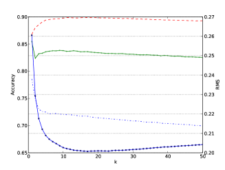
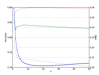
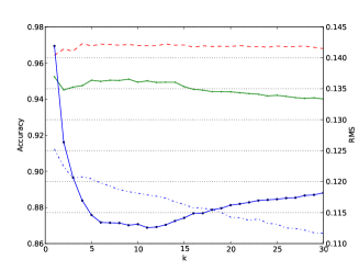
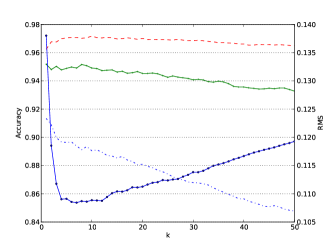
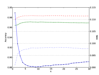
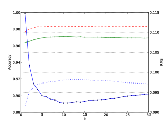
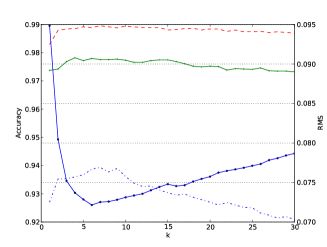
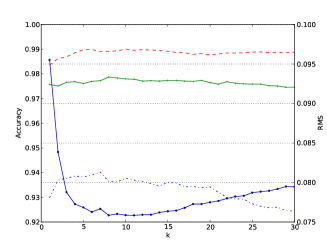
Figure 2: The accuracy within $|\Delta z|<0.1$ (blue dot-dash-line), $|\Delta z|<0.2$ (green solid-line with plus) and $|\Delta z|<0.3$ (red dash-line) and $RMS$ (blue solid-line with dot) as a function of $k$ with the better input patterns for the SDSS sample, the SDSS-UKIDSS sample, the SDSS-WISE sample and SDSS-UKIDSS-WISE sample, respectively. For short, $4C=u-g,g-r,r-i,i-z$; $8C=u-g,g-r,r-i,i-z,z-Y,Y-J,J-H,H-K$; $6C=u-g,g-r,r-i,i-z,z-W1,W1-W2$; $10C=u-g,g-r,r-i,i-z,z-Y,Y-J,J-H,H-K,K-W1,W1-W2$. Left panels: the input pattern is $4C+r$, $8C+r$, $6C+r$, $10C+r$, respectively. Right panels: the input pattern is $4C+i$, $8C+i$, $6C+i$, $10C+i$, respectively.

Table 2: The value of $k$ neighbors for the better patterns for different datasets. $4C=u-g,g-r,r-i,i-z$; $6C=u-g,g-r,r-i,i-z,z-W1,W1-W2$; $8C=u-g,g-r,r-i,i-z,z-Y,Y-J,J-H,H-K$; $10C=u-g,g-r,r-i,i-z,z-Y,Y-J,J-H,H-K,K-W1,W1-W2$.

Data Set	Input Pattern	$k$	$|\Delta z|<0.1$ (%)	$|\Delta z|<0.2$ (%)	$|\Delta z|<0.3$ (%)	$RMS$
SDSS	$4C,r$	17	72.35$\pm$0.33	83.94$\pm$0.21	89.87$\pm$0.30	0.201$\pm$0.003
SDSS	$4C,i$	14	72.50$\pm$0.29	83.92$\pm$0.28	89.83$\pm$0.28	0.201$\pm$0.002
SDSS-UKIDSS	$8C,r$	9	88.58$\pm$0.46	94.90$\pm$0.51	96.88$\pm$0.20	0.115$\pm$0.006
SDSS-UKIDSS	$8C,i$	7	89.17$\pm$0.37	94.69$\pm$0.27	96.91$\pm$0.22	0.115$\pm$0.007
SDSS-WISE	$6C,r$	9	91.58$\pm$0.30	96.49$\pm$0.10	98.33$\pm$0.06	0.090$\pm$0.003
SDSS-WISE	$6C,i$	10	91.74$\pm$0.20	97.02$\pm$0.07	98.31$\pm$0.06	0.093$\pm$0.003
SDSS-UKIDSS-WISE	$10C,r$	7	93.74$\pm$0.52	97.63$\pm$0.21	98.95$\pm$0.25	0.083$\pm$ 0.010
SDSS-UKIDSS-WISE	$10C,i$	5	93.82$\pm$0.44	97.77$\pm$0.21	98.97$\pm$0.28	0.082$\pm$ 0.009

In order to clearly show the difference among different samples, the best predicted results for the four samples are presented in Figure 3. For the SDSS sample, the best input pattern is $4C+r$ as $k=17$; for the SDSS-UKIDSS sample, the best input pattern is $8C+i$ as $k=7$; for the SDSS-WISE sample, the best input pattern is $6C+r$ as $k=9$; and for the SDSS-UKIDSS-WISE sample, the best input pattern is $10C+i$ as $k=5$. Comparisons of spectral redshifts with estimated photometric redshifts are given in the left panel of Figure 3, the distribution of $|\Delta z|$ is shown in the right panel of Figure 3. It clearly shows that there are two clusters in the first scatter plot of the SDSS sample, but they disappear gradually by adding information from more bands, and when using data from all bands in the three surveys, the number of discrete points becomes very small. A small detail should be noticed that the points near the diagonal line in the scatter plot of SDSS-WISE are thicker than that of SDSS-UKIDSS. This indicates that adding WISE infrared bands can help reduce the value of $RMS$ but raise the uncertainty of photometric redshifts again. The influence of the number of bands on the photometric redshift estimation is indicated in Figure 4. The left panel of Figure 4 shows how $RMS$ of $|\Delta z|$ changes with the number of photometric bands for the SDSS-UKIDSS sample (solid line), the SDSS-WISE sample (dashed line) and the SDSS-UKIDSS-WISE sample (dotted line), respectively. The right panel of Figure 4 indicates how percent outliers vary with the number of photometric bands for the SDSS-UKIDSS sample (solid line), the SDSS-WISE sample (dashed line) and the SDSS-UKIDSS-WISE sample (dotted line), respectively. Outliers are defined as objects with $|\Delta z|>0.15$. It is obvious that $RMS$ and percent outliers both usually decrease when the number of photometric bands increases, nevertheless, when the adding parameters have large uncertainty, $RMS$ and percent outliers will rise. As a result, the performance of a algorithm may not necessarily improve when adding more parameters from more bands to predict photometric redshifts.

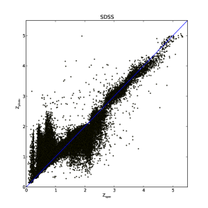
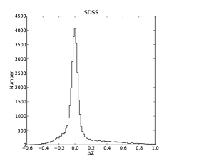
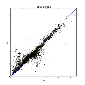
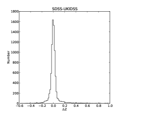
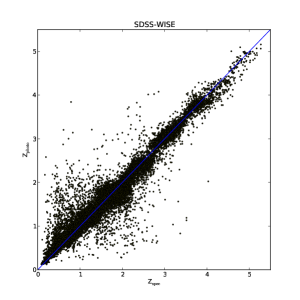
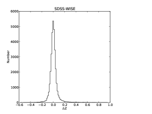
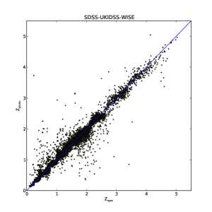
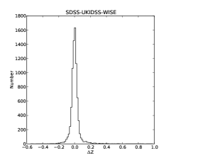
Figure 3: Comparison of photometric redshift estimation results for the SDSS sample with the best input pattern of $4C+r$ as $k=17$; for the SDSS-UKIDSS sample with the best input pattern of $8C+i$ as $k=7$, for the SDSS-WISE sample with the best input pattern of $6C+r$ as $k=9$; and for the SDSS-UKIDSS-WISE sample with the best input pattern of $10C+i$ as $k=5$.

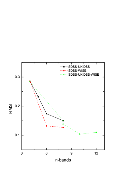
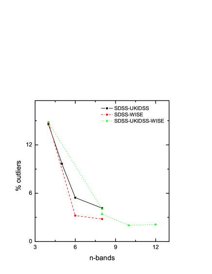
Figure 4: Left panel: $RMS$ of $(z_{\rm phot}-z_{\rm spec})/(1+z_{\rm spec})$ versus the number of photometric bands for the SDSS-UKIDSS sample (solid line), the SDSS-WISE sample (dashed line) and the SDSS-UKIDSS-WISE sample (dotted line), respectively. Right panel: percent outliers versus the number of photometric bands for the SDSS-UKIDSS sample (solid line), the SDSS-WISE sample (dashed line) and the SDSS-UKIDSS-WISE sample (dotted line), respectively.

3.3 Comparison with other algorithms

Various algorithms have been applied on photometric redshift estimation of quasars. The performance of algorithms depends on many factors, such as algorithm itself, model parameters, data, input pattern. It is difficult to say which algorithm is the best. We only think the method is the best for the special data when its model parameters and input pattern are set. For giving a rough comparison of algorithms on this issue, all models we study in this subsection are from WEKA (The Waikato Environment for Knowledge Analysis). WEKA is a tool for data analysis and includes implementations of data pre-processing, classification, regression, clustering, association rules, and visualization by different algorithms. All these algorithms can refer to the book published by Witten & Frank (2005). WEKA’s binaries and sources may be freely available from http://www.cs.waikato.ac.nz/ml/weka/. For our case, the function algorithms implemented include linear regression, Multi-layer perceptron (MLP), pace regression, Radial Basis Function (RBF) network, Support Vector Machines (SVM); lazy learning methods used consist of IB1, IB5 and Locally Weighted Learning (LWL), here IB1 and IB5 all belong to $k$NN, IB1 corresponds to $k$NN when $k=1$ while IB5 points to $k$NN as $k=5$; treelike algorithms applied are REPTree and Decision Stump; so-called “meta” model utilized is bagging; rule models used contain M5-Rules Algorithm and decision table.

The comparison of all models is made on the basis of the following criteria:

i) Correlation Coefficient (also known as $R$): $R$ is a measure of the strength and direction of the linear relationship between two variables that is defined in terms of the (sample) covariance of the variables divided by their (sample) standard deviations.

i) Mean absolute error ($MAE$): MAE is the average of the difference between predicted and actual value in all test cases.

iii) Root Mean-Squared Error ($RMSE$): $RMSE$ is commonly used measure of differences between predicted values (photometric redshifts) by a model and the actually observed values (spectral redshifts). The mean-squared error is one of the most frequently used measures of success for numeric prediction. This value is obtained by computing the average of the squared differences between each computed value and its corresponding correct value. $RMSE$ is just the square root of the mean-squared-error.

Correlation Coefficient ($R$), mean absolute error ($MAE$) and root mean squared error ($RMSE$) is calculated for each machine learning algorithm, respectively. For brief, the input pattern $10C+i$ is taken for all the models. All the experiments are done by 10-fold cross-validation. The comparison of the performance of different algorithms for predicting photometric redshifts of quasars are shown in Table 3. The time to build a model is also depicted in Table 3. As Table 3 indicated, MLP of all function models shows the best performance with the largest value of $R$ and the smallest values of $MAE$ and $RMSE$; IB5 (i.e $k$NN with $k=5$) of lazy learning methods is the best with $R=0.973,MAE=0.096$ and $RMSE=0.186$; REPTree of treelike algorithms is superior to decision stump; M5-rules of rule methods outperforms decision table. Bagging is a popular method that improves the performance for any learning algorithm. The performance of REPTree with bagging algorithm indeed improves compared to REPTree as Table 3 described. Taking no account of lazy learning, the fastest speed to create a training model is pace regression, the second is decision stump, the third belongs to linear regression, however, the three approaches have no good performance for photometric redshift prediction; the slowest is SVM. Considering all algorithms applied here, IB5 shows the best performance. This is why we utilize $k$NN for our case. The advantage of lazy learning is that the training and prediction all delay until a query is made to the system, it deals successfully with changes in the problem domain and it is very useful for large data with few attributes; the disadvantages of lazy learning require the large space to store the entire training data, another disadvantage is that lazy learning approaches are usually slower to predict, though they have a faster training phase. Nevertheless, $k$NN based on KD-Tree improves the speed to evaluate, just like that is done in this paper.

Table 3: Comparison of various methods for photometric redshift estimation of quasars with the input pattern $10C+i$.

Class	Method	$R$	$MAE$	$RMSE$	Time(s)
function	Linear Regression	0.887	0.274	0.369	0.21
	MLP	0.910	0.256	0.360	37.92
	Pace Regression	0.887	0.274	0.369	0.06
	RBF Network	0.395	0.568	0.734	3.26
	SVM	0.884	0.272	0.373	606.61
lazy learning	IB1	0.959	0.112	0.228	0
	IB5	0.973	0.096	0.186	0
	LWL	0.665	0.472	0.567	0
tree	REPTree	0.936	0.140	0.282	0.45
	Decision Stump	0.627	0.498	0.622	0.1
meta	Bagging of REPTree	0.962	0.115	0.219	3.05
rule	Decision Table	0.861	0.260	0.406	3.89
	M5-Rules	0.956	0.128	0.235	59.9

4 CONCLUSIONS

We have demonstrated a simple and useful method $k$-nearest neighbor using multiband data which can effectively estimate photometric redshifts of quasars. According to the above experiments and the comparison with other algorithms, $k$NN can be taken as a powerful tool to determine photometric redshifts of quasars, when it use $k=5$ and ($u-g,g-r,r-i,i-z,z-Y,Y-J,J-H,H-K,K-W1,W1-W2,i$) as the input pattern. On the SDSS-UKIDSS-WISE data set, the accuracy within $|\Delta z|<0.1$ can reaches $93.82\%\pm 0.44\%$, $97.77\%\pm 0.21\%$ within $|\Delta z|<0.2$, $98.97\%\pm 0.28\%$ within $|\Delta z|<0.3$ and $RMS$ is $0.082\pm 0.009$. This method successfully avoids the redshift catastrophic failure when the genuine redshift of quasar is below 2.8. Actually, $k$NN can reach the same level of performance only using cross-match data from the SDSS and UKIDSS databases, but $RMS$ is a little higher (0.115). Adding information from the WISE infrared band can effectively improve the performance of $k$NN on $RMS$. Finally, we improve the performance of $k$NN within $|\Delta z|<0.3$ from 85.19% to about 98.97% and reduce $RMS$ from 0.287 to 0.009. This means that $k$NN using multiband data is an effective and feasible approach for estimating photometric redshifts of quasars. The major advantages of $k$NN are its simplicity and easy understanding without physical assumption. It does not require training, takes the known spectroscopic redshifts as templates and further shows its superiority with large numbers of spectra available. Moreover, the $k$NN approach combined with KD-Tree conquers the high time-consumption faced by traditional $k$NN method.

In the future, the main target is about how to improve the accuracy of photometric redshifts on $|\Delta z|<0.1$. Without doubt, using multibands is a useful and reliable way to improve it and we plan to add ultraviolet band data from GALEX to test this method. Another possible solution is about that $k$NN can be combined with some classification method to conquer the catastrophic failure area on the SDSS optical band that is met by many machine learning algorithms. The work of photometric redshift estimation on optical band is important and urgent because the overlapped area among the several surveys are relatively small and there is over billion of unknown objects with photometric data. We will implement it for predicting the photometric redshifts of quasar candidates for the Guoshoujing Telescope (LAMOST) or other projects in the world.

References

- (1) Abdalla, F. B., Banerji, M., Lahav, O., Rashkov, V., 2011, MNRAS, 417, 1891
- (2) Abazajian, K. N. et al. 2009, ApJS, 182, 543
- (3) Babbedge, T. S. R., Rowan-Robinson, M., Gonzalez-Solares, E., et al. 2004, MNRAS, 353, 654
- (4) Ball, N. M. & Brunner, R. J. 2010, IJMPD, 19, 1049
- (5) Ball, N. M., Brunner, R. J., Myers, A. D., Strand, N. E., Alberts, S. L., Tcheng, D., Llora, X. 2007, ApJ, 663, 774
- (6) Ball, N. M., Brunner, R. J., Myers, A. D., Strand, N. E., Alberts, S. L., Tcheng, D. 2008, ApJ, 683, 12
- (7) Bolzonella, M., Miralles, J.-M., Pelló R. A&A, 2000, 363, 476
- (8) Bovy, J. et al. 2012, ApJ, 749, 41
- (9) Blake, C. et al. 2007, MNRAS, 374, 1527
- (10) Borne, K., in Next Generation of Data Mining (Taylor & Francis: CRC Press), pp. 91-114 (2009)
- (11) Budavri, T., Csabai, I., Szalay, A. S., et al., 2001, AJ, 122, 1163
- (12) Budavri, T., Szalay, A. S., Connolly, A. J., Csabai, I., Dickinson, M. 2000, AJ, 120, 1588
- (13) Collister, A. A. & Lahav, O., 2004, PASP, 116, 345
- (14) Firth, A. E., Lahav, O., Somerville, R. S., 2003, MNRAS, 349, 1397
- (15) Hewett, P. C., Warren, S. J., Croom, S. M. 2008, MNRAS, 365, 1605
- (16) Hall, M., Frank, E., Holmes, G., Pfahringer, B., Reutemann, P., Witten, I. H. 2009, SIGKDD Explorations, 11(1), 10
- (17) Hildebrandt, H., Arnouts, S., Capak, P., et al., 2010, A&A, 523, A31
- (18) Geach, J. E. 2011, MNRAS, 419, 2633
- (19) Kaiser, N. & Aussel, H. 2002, SPIE, 4836, 154
- (20) Kumar, N. D. 2008, Mater Dissertation, St Anne’s College, University of Oxford
- (21) Lawrence, A. et al. 2007, MNRAS, 379, 1599
- (22) Peng, N., Zhang, Y., Zhao, Y., 2010a, Proc. SPIE, 7740, 92
- (23) Peng, N., Zhang, Y., Zhao, Y., 2010b, Proc. SPIE, 7740, 86
- (24) Polsterer, K. L., Zinn, P.-C., Gieseke, F. 2013, MNRAS, 428, 226
- (25) Oyaizu, H., Lima, M., Cunha, C. E., Lin, H., Frieman, J., 2008, ApJ, 674, 768
- (26) Tyson, J. A. 2002, SPIE, 4836, 10
- (27) Wadadekar, Y., et al. 2005, PASP, 117,79
- (28) Wang, D., Zhang, Y., Liu, C., Zhao, Y. 2008, ChJAA, 8(1), 119
- (29) Witten, I. H., Frank, E., Data Mining: Practical Machine Learning Tools and Techniques with Java Implementations, Morgan Kaufmann, San Francisco, 2005
- (30) Laurino, O., D’Abrusco, R., Longo, G., Riccio, G. 2011, MNRAS, 418, 2165
- (31) Warren, S. J., Hewett, P.C., Foltz, C.B. 2000, MNRAS, 312, 827
- (32) Way, M. J., Foster, L. V., Gazis, P. R., Srivastava, A. N. 2009, ApJ, 706, 623
- (33) Richards G. T., et al. 2001, AJ, 122, 1151
- (34) Salvato, M., Hasinger, G., Ilbert, O., et al. 2009, ApJ, 690, 1250
- (35) Salvato, M., Ilbert, O., Hasinger, G., et al. 2011, ApJ, 742, 61
- (36) Schlegel D. J., Finkbeiner D. P., Davis M., 1998, ApJ, 500, 525
- (37) Schneider, D. P., et al. 2010, AJ, 139, 2360
- (38) Weinstein, M. A., et al. 2004, ApJS, 155,243
- (39) Wright, E.L. et al. 2010, AJ, 140, 1868
- (40) Wu, X.-B., Zhang, W., Zhou, X. 2004, ChJAA, 4, 17
- (41) Warren, S. J., Hewett, P. C., Foltz, C. B. 2000, MNRAS, 312,827
- (42) Wu, X.-B. & Jia, Z.-D., 2010, MNRAS, 406, 1583
- (43) Yéche, C. et al. 2010, A&A, 523, A14
- (44) York, D. G., et al. 2000, AJ, 120, 1579
- (45) Zhang, Y., Li, L., Zhao, Y. 2009, MNRAS, 392,233
- (46) Zhang, Y., Zheng, H., Zhao, Y. 2008, Proc. SPIE, 7019, 701938-1