Nonlinear magnetotransport in a dc-current-biased graphene

Abstract

A balance-equation scheme is developed to investigate the magnetotransport in a dc-current-biased graphene. We examine the Shubnikov-de Haas oscillation under a nonzero bias current. With an increase in the current density, the oscillatory differential resistivity exhibits phase inversion, in agreement with recent experimental observation. In the presence of surface optical phonons, a second phase inversion may occur at higher dc bias, due to the reduced influence of electron-heating and the enhanced direct effect of current on differential magnetoresistivity. We also predict the appearance of current-induced magnetoresistance oscillation in suspended graphene at lower magnetic fields and larger current densities. For the graphene mobility currently available ($\approx 20\,{\rm m^{2}/Vs}$), the oscillatory behavior may be somewhat altered by magnetophonon resonance arising from intrinsic acoustic phonon under finite bias current condition.

I introduction

Since its isolation for the first time in 2004,novoselov2004electric graphene, a two-dimensional (2D) single-layer of carbon atoms, has attracted an explosion of interestgeim2007rise ; sarma2010electronic ; goerbig2011electronic due to both its fundamental physics and its potential technological applications. In contrast to ordinary semiconductors, the application of a strong perpendicular magnetic field on pristine graphene results in an energetic quantization proportional to the square root of external magnetic field with the existence of a true zero-energy sharing equally by electrons and holes. As a result, magnetotransport in graphene may exhibits unusual properties. For example, the unique quantum Hall effect in graphene showing half-integer Hall plateaus,zhang2005experimental ; novoselov2007room has become the experimental evidence of massless linear-energy fermionic excitation.

Similarly, the resistivity minima of Shubnikov-de Hass oscillation (SdHO) of graphene appears when filling factor equals $4\left(n+\tfrac{1}{2}\right)$ with $n$ an integer. Recently, Tan et al.tan2011shubnikov found that in addition to the damp of oscillation due to elevated carrier temperature, a phase inversion of the differential magnetoresistivity occurs under dc bias in graphene with relatively low zero-field mobility, i.e. SdHO maxima (minima) invert to minima (maxima). They attributed the observed interesting phenomenon to the elevated electron temperature. The dominant energy dissipation they referred arises from the diffusion of hot carriers to electrodes. However, when a graphene is on a polar substrate, inelastic carrier scattering with surface optical phonons (SO phonons) is important and offers an intrinsic energy-dissipation mechanism.fratini2008substrate ; li2010influence ; zhu2009carrier This notable phase-inversion effect has also been observed experimentally in usual two-dimensional electron gas (2DEG) with high mobility.kalmanovitz2008warming So far, a microscopic theoretical analysis including carrier–phonon scattering effect on dc-current-induced phase inversion of SdHO has still been lacking even for parabolic energy-band system.

The magnetoresistance oscillation directly induced by a dc current, periodic in current density and in inverse magnetic field, is another noteworthy nonlinear transport phenomenon, which was first observed a decade ago in conventional 2DEG.yang2002zener ; bykov2005effect The effect is ascribed to the Zener tunneling between Hall-field-tilted Landau levels due to short-range (SR) impurity scattering.yang2002zener ; zhang2007magnetotransport Later, by including inelastic phonon scattering, a microscopic balance-equation scheme has been constructed, conveniently accounting for this current-induced nonlinear transport phenomenon with considering the electron heating.lei2007current So far, however, investigations of nonlinear magnetoresistance oscillation have been carried out only for high-mobility 2DEGs with parabolic energy dispersion.yang2002zener ; zhang2007magnetotransport ; bykov2005effect ; lei2007current ; zhang2007effect ; vavilov2007 Owing to the absence of much of extrinsic impurities and SO phonons, the suspended graphene can achieve relatively high mobilitybolotin2008ultrahigh ; bolotin2008temperature that Landau levels can be well resolved even in quite a weak magnetic field. Hence, it is expected that this kind of nonlinear magnetoresistance oscillation could been observed in suspended graphene. Therefore, an efficient scheme capable of dealing with magnetotransport in graphene under an external current bias is in sore need.

The balance-equation approach, which is especially suitable to deal with current-controlled nonlinear transport, was established based on the separation of the center-of-mass motion from the relative carrier motion in parabolic energy-band systems.lei1985gsf ; lei1985tdb ; cai1985 ; lei1987nonlinear ; lei2008balance It turns out that this scheme can be applied to systems with linear energy dispersion.wang2012linear In this paper, we will generalize this scheme to graphene subject to a magnetic field and a finite dc current. The paper is organized as follows. In Sec. II, the force- and energy-balance equations are derived for graphene in the presence of normal magnetic field and external dc current. The effect of a finite dc bias on the SdHO in a graphene on a SiO₂ substrate is investigated in Sec. III.1. The current-control magnetoresistance oscillation in a suspended graphene is discussed in Sec. III.2. A summary is given in Sec. IV. The derivation of energy-balance equation is presented in Appendix.

II Balance-Equation Formulation

We consider a single layer graphene in the $x$-$y$ plane under the influence of a uniform magnetic field ${\bm{B}}=B\hat{z}$ along the $z$ direction and a dc electric field ${\bm{E}}=(E_{x},E_{y})$ applied in the layer plane. The carriers having enough density near the $K$ or $K^{\prime}$ points in the graphene, are interacting with each other, coupled with lattice vibrations of the graphene as well as the oxide interface, and scattered by randomly located disorders. The Hamiltonian of this system consists of an carrier part $\mathcal{H}_{\rm e}$, a phonon part $\mathcal{H}_{\rm ph}$, and carrier–impurity and carrier–phonon interactions $\mathcal{H}_{\rm ei}$ and $\mathcal{H}_{\rm ep}$:

$$\mathcal{H}=\mathcal{H}_{\rm e}+\mathcal{H}_{\rm ph}+\mathcal{H}_{\rm ei}+\mathcal{H}_{\rm ep}.$$ (1)

Here, the carrier Hamiltonian can be written as

$$\mathcal{H}_{\rm e}=\sum_{j,\alpha}\left[v_{\rm F}(\pi_{j}^{x}\sigma_{j}^{x}+c_{\alpha}\pi_{j}^{y}\sigma_{j}^{y})+e\bm{r}_{j}\cdot\bm{E}\right],$$ (2)

where ${\bm{r}}_{j}=(x_{j},y_{j})$, ${\bm{p}}_{j}=(p_{jx},p_{jy})$, ${\bm{\pi}}_{j}\equiv\bm{p}_{j}+e\bm{A}(\bm{r}_{j})=(\pi_{j}^{x},\pi_{j}^{y})$, and ${\bm{\sigma}}_{j}=(\sigma_{j}^{x},\sigma_{j}^{y},\sigma_{j}^{z})$, stand, respectively, for the coordinate, momentum, canonical momentum, and Pauli operators of the $j$th carrier in the pseudospin space formed by the A and B sublattices; $c_{\alpha}$ is a valley-related coefficient equaling $+1$ or $-1$ for carrier in $\alpha=K$ or $K^{\prime}$ valley; $\bm{A}(\bm{r})=(-By,0)$ is the vector potential of the magnetic field in the Landau gauge; $v_{\rm F}=1.1\times 10^{6}\,{\rm m/s}$ is the Fermi velocity. The forms of $\mathcal{H}_{\rm ei}$ and $\mathcal{H}_{\rm ep}$ are similar to those given in Refs. lei1987nonlinear, and lei2008balance, , without intervalley transition of carriers.

In the frame work of balance equation approach,lei1985tdb ; lei1985gsf ; cai1985 we introduce the 2D center-of-mass (c.m.) momentum and coordinate $\bm{P}_{\alpha}=\sum_{j\in\alpha}\bm{p}_{j}$ and $\bm{R}_{\alpha}=N^{-1}_{\alpha}\sum_{j\in\alpha}\bm{r}_{j}$, and the relative-carrier momenta and coordinates $\bm{p}^{\prime}_{j}=\bm{p}_{j}-\bm{P}_{\alpha}/N_{\alpha}$ and $\bm{r}_{j}^{\prime}=\bm{r}_{j}-\bm{R}_{\alpha}$ for carriers in the $\alpha$ valley having carrier number $N_{\alpha}$, to write the Hamiltonian $\mathcal{H}_{\rm e}$ into the sum of a single-particle c.m. part $\mathcal{H}_{\rm cm}=\sum_{\alpha}\mathcal{H}_{\rm cm}^{\alpha}$ and a many-particle relative-carrier part $\mathcal{H}_{\rm er}=\sum_{\alpha}\mathcal{H}_{\rm er}^{\alpha}$: $\mathcal{H}_{\rm e}=\mathcal{H}_{\rm cm}+\mathcal{H}_{\rm er}$, with

$$\mathcal{H}_{\rm cm}^{\alpha} =v_{\rm F}(\varPi^{\alpha}_{x}\sigma_{\alpha{\rm c}}^{y}+c_{\alpha}\varPi^{\alpha}_{y}\sigma_{\alpha{\rm c}}^{x})+N_{\alpha}e{\bm{E}}\cdot\bm{R}_{\alpha},$$ (3)

$$\mathcal{H}_{\rm er}^{\alpha} =\sum_{j\in\alpha}\left[v_{\rm F}(\pi_{j}^{\prime x}\sigma_{j}^{y}+c_{\alpha}\pi_{j}^{\prime y}\sigma_{j}^{x})\right].$$ (4)

In this, ${\bm{\varPi}}^{\alpha}\equiv\bm{P}_{\alpha}+N_{\alpha}e\bm{A}(\bm{R}_{\alpha})=(\varPi_{x}^{\alpha},\varPi_{y}^{\alpha})$ is the center-of-mass canonical momentum of the $\alpha$ valley and ${\bm{\pi}}_{j}^{\prime}\equiv\bm{p}_{j}^{\prime}+e\bm{A}(\bm{r}_{j}^{\prime})=(\pi_{j}^{\prime x},\pi_{j}^{\prime y})$ is the canonical momentum for the $j$th relative carrier. Here we have also introduced c.m. spin operators ${\sigma}_{\alpha\rm c}^{x}\equiv N_{\alpha}^{-1}\sum_{j\in\alpha}\sigma_{j}^{x}$ and ${\sigma}_{\alpha\rm c}^{y}\equiv N_{\alpha}^{-1}\sum_{j\in\alpha}\sigma_{j}^{y}$ for the $\alpha$ valley. The commutation relations between the c.m. Pauli operators $\sigma_{\alpha\rm c}^{x}$ and $\sigma_{\alpha\rm c}^{y}$ and the Pauli operators $\sigma_{j}^{x}$ and $\sigma_{j}^{y}$ of the $j$th carrier are of order of $1/N_{\alpha}$. Therefore, for a macroscopically large $N_{\alpha}$ system, the c.m. part $\mathcal{H}_{\rm cm}$ actually commutes with the relative-carrier part $\mathcal{H}_{\rm er}$ in the Hamiltonian, i.e. the c.m. motion and the relative motion of carriers are truly separated from each other. The couplings between the two emerge only through the carrier–impurity and carrier–phonon interactions. Furthermore, the electric field ${\bm{E}}$ shows up only in $\mathcal{H}_{\rm cm}$. And, in view of $[r^{\prime}_{i\beta_{1}},p^{\prime}_{j\beta_{2}}]={\rm i}\delta_{\beta_{1}\beta_{2}}(\delta_{ij}-1/N_{\alpha})\simeq{\rm i}\delta_{\beta_{1}\beta_{2}}\delta_{ij}$, i.e. the relative-carrier momenta and coordinates can be treated as canonical conjugate variables, the relative-motion part $\mathcal{H}_{\rm er}^{\alpha}$ is just the Hamiltonian of $N_{\alpha}$ carriers in the $\alpha$ valley of graphene in the magnetic field without electric field.

In terms of the c.m. coordinate ${\bm{R}}_{\alpha}$ and the relative carrier density operator $\rho_{\bm{q}}^{\alpha}=\sum_{j\in\alpha}{e}^{{\rm i}\,{\bm{q}}\cdot{\bm{r}}^{\prime}_{j}}$, the carrier–impurity and carrier–phonon interactions can be written aslei1985tdb ; cai1985

$$\mathcal{H}_{\rm ei}= \sum_{\alpha,{\bm{q}},a}U({\bm{q}})\,{e}^{{i}\,{\bm{q}}\cdot\left({\bm{R}}_{\alpha}-{\bm{r}}_{a}\right)}\rho_{\bm{q}}^{\alpha},$$ (5)

$$\mathcal{H}_{\rm ep}= \sum_{\alpha,{\bm{q}},\nu}M({\bm{q}},\nu)\,\varphi_{{\bm{q}}\nu}{e}^{{i}\,{\bm{q}}\cdot{\bm{R}}_{\alpha}}\rho_{\bm{q}}^{\alpha}.$$ (6)

Here $U({\bm{q}})$ and $M({\bm{q}},\nu)$ are, respectively, the impurity potential (an impurity at randomly distributed position ${\bm{r}}_{a}$) and carrier–phonon coupling matrix element in the plane-wave representation, and $\varphi_{{\bm{q}}\nu}\equiv b_{{\bm{q}}\nu}+b_{-{\bm{q}}\nu}^{\dagger}$ is the phonon field operator with $b_{{\bm{q}}\nu}^{\dagger}$ and $b_{{\bm{q}}\nu}$ being the creation and annihilation operators for a 2D phonon of wavevector ${\bm{q}}$ in the branch $\nu$ having frequency ${\it\Omega}_{{\bm{q}}\nu}$.

The derivation of balance equations starts by noticing that the c.m. velocity (operator) ${\bm{V}}_{\alpha}$ is the time variation of its coordinate: ${\bm{V}}_{\alpha}=\dot{\bm{R}}_{\alpha}=-{i}[{\bm{R}}_{\alpha},\mathcal{H}]=v_{\rm F}(\sigma_{\alpha\rm c}^{y}\,\hat{i}+c_{\alpha}\sigma_{\alpha\rm c}^{x}\,\hat{j})$, and proceeds from the Heisenberg equations for the rate of change of the center-of-mass canonical momentum $\dot{\bm{\varPi}}_{\alpha}=-i[\bm{\varPi}_{\alpha},\mathcal{H}]$, and that of the relative-carrier energy $\dot{\mathcal{H}}_{\rm er}^{\alpha}=-i[\mathcal{H}_{\rm er}^{\alpha},\mathcal{H}]$. The statistical average of the above operator equations can be determined to linear order in the carrier–impurity and carrier–phonon interactions $\mathcal{H}_{\rm ei}$ and $\mathcal{H}_{\rm ep}$ using the initial density matrix $\hat{\rho}_{0}=Z^{-1}e^{-\mathcal{H}_{\rm ph}/T}e^{-\mathcal{H}_{\rm er}/T_{\rm e}}$ with lattice temperature $T$ and a common carrier temperature $T_{\rm e}$ for carriers in both valleys in view of the symmetry of graphene band structure, which give rise to equal carrier number densities $N_{K}=N_{K^{\prime}}$ and equal average c.m. velocities ${\bm{v}}={\bm{v}}_{\alpha}=\langle{\bm{V}}_{\alpha}\rangle$ ($\alpha=K,K^{\prime}$).

Steady-state transport balance equations are obtained by setting $\sum_{\alpha}\langle\dot{\bm{\varPi}}_{\alpha}\rangle=0$ and $\sum_{\alpha}\langle\dot{\mathcal{H}}_{\rm er}^{\alpha}\rangle=0$. The derived force and energy balance equations, which are identical for both valleys, can be written (for graphene system of unit area) as

$$0= -Ne\bm{v}\times\bm{B}-Ne\bm{E}+\bm{f}_{\rm i}+\bm{f}_{\rm p},$$ (7)

$$0= (\bm{f}_{\rm i}+\bm{f}_{\rm p})\cdot\bm{v}+w.$$ (8)

Derivation of energy-balance equation is given in appendix. Here $N=\sum_{\alpha}N_{\alpha}$ is the total number density of carriers (in both valleys) for system of unity area, ${\bm{f}}_{\rm i}$ and ${\bm{f}}_{\rm p}$ are total frictional forces experienced by the center of mass due to impurity and phonon scatterings:

$$\bm{f}_{\rm i}= n_{\rm i}\sum_{\bm{q}}\left|U(\bm{q})\right|^{2}\bm{q}\varPi_{2}(\bm{q},\omega_{0}),$$ (9)

$$\bm{f}_{\rm p}= \sum_{\bm{q},\nu}\left|M(\bm{q},\nu)\right|^{2}\bm{q}\varPi_{2}(\bm{q},{\it\Omega}_{\bm{q}\nu}+\omega_{0})$$

$$\hskip 11.38092pt\times\left[n\Big{(}\frac{{\it\Omega}_{\bm{q}\nu}}{T}\Big{)}-n\Big{(}\frac{{\it\Omega}_{\bm{q}\nu}+\omega_{0}}{T_{\rm e}}\Big{)}\right],$$ (10)

and $w$ is the rate of carrier energy-dissipation to the lattice due to carrier–phonon interactions:

$$w= \sum_{\bm{q},\nu}\left|M(\bm{q},\nu)\right|^{2}{\it\Omega}_{\bm{q}\nu}\varPi_{2}(\bm{q},{\it\Omega}_{\bm{q}\nu}+\omega_{0})$$

$$\hskip 11.38092pt\times\left[n\Big{(}\frac{{\it\Omega}_{\bm{q}\nu}}{T}\Big{)}-n\Big{(}\frac{{\it\Omega}_{\bm{q}\nu}+\omega_{0}}{T_{\rm e}}\Big{)}\right].$$ (11)

In these equations $n_{\rm i}$ is the impurity density, $n(x)=(e^{x}-1)^{-1}$ is the Bose distribution function, $\omega_{0}\equiv{\bm{q}}\cdot{\bm{v}}$, $\varPi_{2}(\bm{q},\omega)=\sum_{\alpha}\varPi_{2}^{\alpha}(\bm{q},\omega)$ with $\varPi_{2}^{\alpha}(\bm{q},\omega)$ standing for the imaginary part of the Fourier spectrum of the relative-carrier density correlation function of the $\alpha$ valley in the magnetic field defined by

$$\varPi^{\alpha}({\bm{q}},t-t^{\prime})=-{i\,}\theta(t-t^{\prime})\big{\langle}\big{[}\rho_{\bm{q}}^{\alpha}(t),\,\rho_{-{\bm{q}}}^{\alpha}(t^{\prime})\big{]}\big{\rangle}_{0},$$ (12)

where $\rho_{\bm{q}}^{\alpha}(t)={\rm e}^{{i\,}\mathcal{H}_{\rm er}t}\rho_{\bm{q}}^{\alpha}\,{\rm e}^{-{i\,}\mathcal{H}_{\rm er}t}$ and $\langle...\rangle_{0}$ denotes the statistical averaging over the initial density matrix $\hat{\rho}_{0}$.lei1985gsf ; lei2008balance

In the magnetic field the imaginary part of the relative-carrier density correlation function $\varPi_{2}(\bm{q},\omega)$ can be calculated in the Landau representation.ting1977theory The eigenstates of the single-particle Hamiltonian $h^{\alpha}=v_{\rm F}(\pi^{x}\sigma^{x}+c_{\alpha}\pi^{y}\sigma^{y})$ in the magnetic field $B\hat{z}$ can be specified by a set of quantum numbers $\{n,k_{x},\sigma,\lambda,\alpha\}$ with $n$, $k_{x}$, $\sigma$, and $\lambda$ denoting the Landau index, the $x$ component of the wave vector, the pseudospin index, and the band index (electron $\lambda=1$ or hole $\lambda=-1$), respectively. The eigenenergies of $h^{\alpha}$ are

$$\varepsilon_{\lambda n}=\lambda v_{\rm F}\sqrt{2eBn}=\lambda\varepsilon_{n}\,\,\,(n=0,1,2,...),$$ (13)

which is pseudospin- and valley-degenerate. The corresponding eigenfunctions can be written as $\Psi_{nk_{x}\sigma}^{\alpha\lambda}=\psi_{nk_{x}}^{\alpha\lambda}\otimes\chi_{\sigma}$ with $\chi_{\sigma}$ standing for the eigenstate of Pauli matrix $\sigma_{z}$ and

$$\psi_{nk_{x}}^{K\lambda}(\bm{r})=\frac{e^{ik_{x}x}}{\sqrt{1+s_{n}}}\left(\begin{array}[]{c}-\lambda s_{n}\phi_{{n-1},k_{x}}(y)\\ \phi_{n,k_{x}}(y)\\ \end{array}\right),$$ (14)

$$\psi_{nk_{x}}^{K^{\prime}\lambda}(\bm{r})=\frac{e^{ik_{x}x}}{\sqrt{1+s_{n}}}\left(\begin{array}[]{c}\phi_{{n},k_{x}}(y)\\ -\lambda s_{n}\phi_{{n-1},k_{x}}(y)\\ \end{array}\right).$$ (15)

Here $s_{n}=1-\delta_{n,0}$ and $\phi_{n,k_{x}}(y)$ is the harmonic oscillator eigenfunction:

$$\phi_{n,k_{x}}(y)=\frac{1}{\sqrt{2^{n}n!l_{\rm B}\sqrt{\pi}}}\exp\left[-\frac{(y-y_{c})^{2}}{2l_{\rm B}^{2}}\right]H_{n}\left(\frac{y-y_{c}}{l_{\rm B}}\right),$$ (16)

with $H_{n}(x)$ the Hermite polynomial, $l_{\rm B}=\sqrt{1/(eB)}$ and $y_{c}=k_{x}/(eB)$.

The $\varPi_{2}(\bm{q},\omega)$ can be expressed in the Landau-representation in the formwang2012linear ; roldan2009 ; Pyatkovskiy

$$\varPi_{2}(\bm{q},\omega)\!=\!\frac{g_{s}g_{v}}{2\pi l_{\rm B}^{2}}\sum_{\begin{subarray}{c}n,n^{\prime}\\ \lambda,\lambda^{\prime}\end{subarray}}C_{n,n^{\prime}}^{\lambda,\lambda^{\prime}}\big{(}\frac{l_{\rm B}^{2}q^{2}}{2}\big{)}\varPi_{2}(n,n^{\prime};\lambda,\lambda^{\prime};\omega),$$ (17)

$$\varPi_{2}(n,n^{\prime};\lambda,\lambda^{\prime};\omega)= -\frac{1}{\pi}\int d\epsilon[f(\epsilon)-f(\epsilon+\omega)]$$

$$\hskip 5.69046pt\times{\rm Im}G_{\lambda n}(\epsilon+\omega){\rm Im}G_{\lambda^{\prime}n^{\prime}}(\epsilon).$$ (18)

Note that despite different forms of wave functions the $\varPi_{2}(n,n^{\prime};\lambda,\lambda^{\prime};\omega)$ function and the transform factor $C_{n,n^{\prime}}^{\lambda,\lambda^{\prime}}(l_{\rm B}^{2}q^{2}/2)$ are identical for both valleys and for both pseudospin directions, whence the valley and spin summations just give rise to the multiplication of degenerate constants $g_{v}=g_{s}=2$. Here the transform factor

$$C_{n,n^{\prime}}^{\lambda,\lambda^{\prime}}(x)= \frac{x^{n_{2}-n_{1}}e^{-x}}{(1+s_{n})(1+s_{n^{\prime}})}\frac{n_{1}!}{n_{2}!}\bigg{[}L_{n_{1}}^{n_{2}-n_{1}}(x)$$

$$\hskip 28.45274pt+\lambda\lambda^{\prime}s_{n}s_{n^{\prime}}\sqrt{\frac{n_{2}}{n_{1}}}L_{n_{1}-1}^{n_{2}-n_{1}}(x)\bigg{]}^{2},$$ (19)

with $n_{1}={\rm min}(n,n^{\prime})$, $n_{2}={\rm max}(n,n^{\prime})$, and $L_{n}^{m}(x)$ being associated Laguerre polynomials.

The Landau levels are broadened due to impurity, phonon and carrier-carrier scatterings. We model the imaginary part of the retarded Green’s function ${\rm Im}G_{\lambda n}(\epsilon)$ in Eq. (II), or the density-of-state (DOS) of the $\lambda n$th Landau level, using a Gaussian formAndo1982

$${\rm Im}G_{\lambda n}(\epsilon)=-\frac{\sqrt{2\pi}}{\varGamma_{\lambda n}}\exp\left[-\frac{2(\epsilon-\varepsilon_{\lambda n})^{2}}{\varGamma_{\lambda n}^{2}}\right],$$ (20)

with a half-widthZheng2002

$$\varGamma_{\lambda n}=\left[{2\omega_{\lambda n}}/({\pi\tau_{s}})\right]^{1/2},$$ (21)

where $\tau_{s}$ is the single-particle lifetime and $\omega_{\lambda n}=|\varepsilon_{\lambda n+1}-\varepsilon_{\lambda n}|$ is the level distance or the cyclotron frequency of the $\lambda n$th Landau level, with $\omega_{\lambda n}\approx v_{\rm F}(eB/2n)^{1/2}=eBv_{\rm F}^{2}/\varepsilon_{n}$ for large $n$ irrespective of the band index, giving rise to valley- and band-independent broadening $\varGamma_{\lambda n}=\varGamma_{n}$.

In the following we restrict ourselves to the $n$-doped case at relatively low temperature, i.e., the carriers are electrons, that we only need to consider states with band index $\lambda=1$. For conciseness we will no longer write out the band index $\lambda$ in the expressions and equations and denote $\varPi_{2}(n,n^{\prime};1,1;\omega)$, $C_{n,n^{\prime}}^{1,1}(x)$, and ${\rm Im}G_{1n}(\epsilon)$ simply as $\varPi_{2}(n,n^{\prime};\omega)$, $C_{n,n^{\prime}}(x)$ and ${\rm Im}G_{n}(\epsilon)$. The Landau-level summation indices $n$ and $n^{\prime}$ in all the equations are taken over $0,1,2,...$ but the ${\rm Im}G_{0}(\epsilon)$ function should be replaced by ${\rm Im}G_{0}^{p}(\epsilon)=\theta(\epsilon){\rm Im}G_{0}(\epsilon)$ due to electron-hole symmetry of the band structure.wang2012linear

The total electron number density $N$ is related to the chemical potential $\varepsilon_{f}$ of the Landau quantized graphene system by the equation

$$N=-\frac{g_{s}g_{v}}{2(\pi l_{\rm B})^{2}}\sum_{n}\int d\epsilon f(\epsilon){\rm Im}G_{n}(\epsilon),$$ (22)

in which $f(\epsilon)=\{\exp[(\epsilon-\varepsilon_{f})/T_{\rm e}]+1\}^{-1}$ is the Fermi distribution function at electron temperature $T_{\rm e}$.

Force- and energy-balance equations (7) and (8), in which the frictional forces ${\bm{f}}_{\rm i}$, ${\bm{f}}_{\rm p}$ and the electron dissipation rate $w$ are functions of carrier drift velocity ${\bm{v}}$ and electron temperature $T_{\rm e}$, describe the steady-state nonlinear magnetotransport in the graphene. With given carrier drift velocity ${\bm{v}}$ or the dc current density ${\bm{J}}=Ne{\bm{v}}$, the electron temperature $T_{\rm e}$ can be determined by the energy-balance equation, and the magnetoresistance is obtained from force-balance equation. Note that the frictional forces $\bm{f}_{\rm i}$ and $\bm{f}_{\rm p}$ are in the opposite direction of the drift velocity $\bm{v}$ and their magnitudes are functions of $v=|{\bm{v}}|$ only: ${\bm{f}}_{\rm i}=-{\bm{v}}f_{\rm i}(v)/v$ and ${\bm{f}}_{\rm p}=-{\bm{v}}f_{\rm p}(v)/v$. In the Hall configuration, e.g. with a drift velocity $\bm{v}=(v,0)$ in the $x$ direction, the force-balance equation Eq. (7) yields a transverse resistivity $R_{xy}=-E_{y}/(Nev)=-B/(Ne)$, a longitudinal resistivity $R_{xx}=-E_{x}/(Nev)=-(f_{\rm i}+f_{\rm p})/(N^{2}e^{2}v)$, and a longitudinal differential resistivity $r_{xx}=-(N^{2}e^{2})^{-1}d(f_{\rm i}+f_{\rm p})/dv$.

III Numerical calculations and discussions

We will use a phenomenological parameter $\alpha_{\Gamma}$ to relate the single particle lifetime $\tau_{s}$ to the transport scattering time in the system:lei2003radiation $\tau_{\rm tr}=\alpha_{\Gamma}\tau_{s}$, and, by expressing $\tau_{\rm tr}$ with the zero-field mobility $\mu$,hwang2007 ; wang2011 we can write the Landau-level broadening in the vicinity of Fermi energy $\varepsilon_{\rm F}=v_{\rm F}\sqrt{\pi N}$ as

$$\varGamma=(ev_{\rm F}/\pi)[2B\alpha_{\Gamma}/(N\mu)]^{1/2}.$$ (23)

The broadening parameter will be taken to be $\alpha_{\Gamma}=2$ throughout the calculation.

We consider two cases: a graphene monolayer on a SiO₂ substratetan2011shubnikov and a suspended monolayer graphene. The electrons in graphene are scattered by charged impurities distributed at a distance $d$ from the layer with $d=4\,{\rm\AA}$ for the graphene on SiO₂ substrate and $d=0$ for the suspended one, having a scattering potential

$$U(\bm{q})=\frac{Ze^{2}}{2\epsilon_{0}\kappa_{\rm avg}q}e^{-qd}.$$ (24)

Here $\kappa_{\rm avg}$ is the average dielectric constant of two regions (air and SiO₂ or air) surrounding the graphene. Henceaniruddha2010effect ; Fischetti $\kappa_{\rm avg}\approx(1+\kappa)/2=2.45$ for non-suspended graphene ($\kappa=3.9$ is the static dielectric constant of SiO₂), while $\kappa_{\rm avg}\approx 1$ for suspended one.

For intrinsic acoustic phonon scatterings in the graphene layer, there are two 2D modes, the sum of which can be treated as isotropic oneVasili2010inelastic ; Raseong2011 with a scattering matrix element

$$|M(\bm{q},{\rm AC})|^{2}=\frac{D^{2}q}{2\rho_{m}v_{\rm ph}},$$ (25)

and an averaged sound velocityHwang2008acoustic $v_{\rm ph}=2\times 10^{4}\,{\rm m/s}$. We choose the deformation potential constant as a moderate valueHwang2008acoustic ; chen2008intrinsic $D=19\,{\rm eV}$ and the mass density $\rho_{m}=7.6\times 10^{-8}\,{\rm g/cm^{2}}$.Hwang2008acoustic

The electrons can also be scattered by the intrinsic optical phonons in graphene. However, the energies of these intrinsic optical modes are greater than $150\,{\rm meV}(\approx 1740\,{\rm K})$, which is much larger than the lattice and electron temperatures concerned and can be neglected. For graphene on the SiO₂ substrate, the surface optic phonon couples to the electrons in graphene by an effective electric field. Due to small van der Waals distance between the polar substrate and the interface, the 2D surface optical (SO) phonon plays a more prominent role in transport in graphene than in usual heterojunctions. The coupling matrix element can be written asfratini2008substrate

$$|M(\bm{q},{\rm SO})|^{2}=\frac{e^{2}\varOmega_{\rm so}}{2\epsilon_{0}q}\left(\frac{1}{\kappa_{\infty}+1}-\frac{1}{\kappa+1}\right)e^{-2qd},$$ (26)

where $\varOmega_{\rm so}$ is the frequency of SO phonon and $\kappa_{\infty}$ is the optical dielectric constant of substrate. For SiO₂, $\kappa_{\infty}=2.4$ and there are two SO-phonon modes having frequenciesFischetti $\varOmega_{\rm so}^{(1)}=59\,{\rm meV}$ and $\varOmega_{\rm so}^{(2)}=155\,{\rm meV}$. The second mode is negligible in the present study owing to its large frequency.

III.1 SdHO under nonzero dc current

In order to study the SdHO under a finite bias dc current in graphene we calculate the magnetoresistivity of a graphene monolayer on a SiO₂ substrate having electron density $N=3.16\times 10^{12}\,{\rm cm^{-2}}$ and zero-magnetic-field mobility $\mu=0.8\,{\rm m^{2}/Vs}$ in the magnetic fields ranging from 0 to 15 T at lattice temperature $T=2\,{\rm K}$ on the basis of balance equations (7) and (8). The calculated longitudinal magnetoresistivity $R_{xx}$ and differential magnetoresistivity $r_{xx}$ are shown in Fig. 1(a) and Fig. 1(b) as functions of the magnetic field $B$ for different given current densities $J$. The standard SdHO curves of graphene are obtained, where the valleys of magnetoresistivity $R_{xx}$ locate at the magnetic fields corresponding to the half-integer filling factorszhang2005experimental ; tan2011shubnikov $\nu=\tfrac{2\pi N}{eB}=4(n+\tfrac{1}{2})$ with $n=2,3,4,...,$ as indicated in the figure. The increasing current density suppresses the oscillation, while the peak/valley positions remain essentially unchanged. The significant feature of current-related SdHO appears in the differential resistivity as shown in Fig. 1(b). With the rise of current density, the oscillation of differential resistivity $r_{xx}$ not only tends to decrease its amplitude, but, more prominently, exhibits phase inversion, e.g., SdHO minima (maxima) invert to maxima (minima) at certain value of bias current density, which is roughly linearly dependent on the magnetic field of the SdHO extrema. These features are in good agreement with the experimental observation.tan2011shubnikov

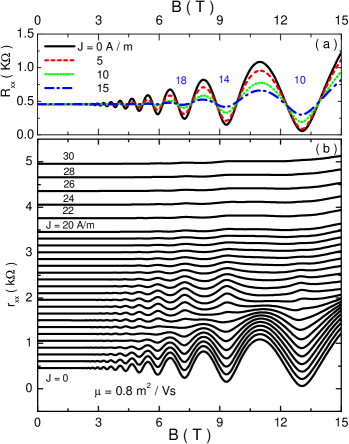
Figure 1: (Color online) (a) Magnetoresistivity $R_{xx}$ is shown versus magnetic field $B$ at various dc current densities $J=$0, 5, 10, 15$\,{\rm A/m}$. The integers near the valleys indicate the filling factors. (b) Differential magnetoresistivity $r_{xx}$ is plotted as a function of the magnetic field for various current densities at lattice temperature $T=2\,{\rm K}$. These $r_{xx}$ curves of different $J$ values are vertically offset for clarity. The current densities are $J=0$, 1, 2, $\cdots$, 20$\,{\rm A/m}$ in 1$\,{\rm A/m}$ step for the lower 21 ones, or are indicated in the figure for others. The system is a monolayer graphene on a SiO₂ substrate having electron density $N=3.16\times 10^{12}\,{\rm cm^{-2}}$ and zero-magnetic-field mobility $\mu=0.8\,{\rm m^{2}/Vs}$.

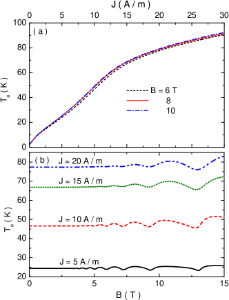
Figure 2: (Color online) Electron temperature $T_{\rm e}$ is shown as a function of dc bias current density at various magnetic fields (a) and as a function of magnetic field at various bias current densities (b) for the same system as described in Fig. 1.

The phase inversion of SdHO is closely related to the rise of electron temperature with increasing bias current. Fig. 2 shows the calculated electron temperature $T_{\rm e}$ as a function of the bias current density $J$ at magnetic field strengths $B=6,8$, and $10$ T (a), as well as $T_{\rm e}$ versus $B$ at current densities $J=5,10,15,20$ A/m (b). When current density is lower than 12 A/m, the electron temperature almost linearly depends on the dc bias. For higher current density, the enhanced energy dissipation arising from electron–SO-phonon interaction restrains the linear increase of electron temperature. In the fixed bias current case (b), only a small oscillation of electron temperature around a certain value shows up for almost the whole magnetic field range presented in the figure.

In the balance-equation scheme, the frictional forces $f_{\rm i}$ and $f_{\rm p}$ are functions of the drift velocity $v$ (i.e. the current density $J=Nev$) and the electron temperature $T_{\rm e}$, and the latter is determined as a function of $v$ from the energy balance equation. Therefore the differential resistivity derived can be expressed as

$$r_{xx} =R_{xx}+J\frac{\partial R_{xx}}{\partial T_{\rm e}}\frac{\partial T_{\rm e}}{\partial J}+J\frac{\partial R_{xx}}{\partial J},$$

$$=R_{xx}+r_{xx}^{T_{\rm e}}+r_{xx}^{v},$$ (27)

where $r_{xx}^{T_{\rm e}}$ can be thought as the part arising from the electron-temperature change and $r_{xx}^{v}$ as that direct from current-density change. We plot the calculated $R_{xx}$, $r_{xx}^{T_{\rm e}}$ and $r_{xx}^{v}$, as well as the total $r_{xx}$, as functions of the magnetic field $B$ for several bias current densities $J=4,8,12,16$, and $20$ A/m in Fig. 3. The three constituent parts $R_{xx}$, $r_{xx}^{T_{\rm e}}$ and $r_{xx}^{v}$ all exhibit oscillations having extrema at positions $\nu=4(n+\tfrac{1}{2})$. However, the phase of $r_{xx}^{T_{\rm e}}$ is opposite to those of $R_{xx}$ and $r_{xx}^{v}$. Note that in the current range $0<J<12\,{\rm A/m}$, when SO-phonons play a relatively small role in dissipating energy, the electron temperature grows almost linearly with increasing current density and $|r_{xx}^{v}|$ is one order of magnitude smaller than $|R_{xx}|$ or $|r_{xx}^{T_{\rm e}}|$, hence, $R_{xx}$ and $r_{xx}^{T_{\rm e}}$ constitute dominant contributions to total $r_{xx}$ and the current-induced electron temperature rising accounts for the phase inversion of $r_{xx}$ in this current density regime, as pointed out by Tan et al.tan2011shubnikov

With further increase in the current density, $R_{xx}$ decreases, while $r_{xx}^{T_{\rm e}}$ first ascends and then descends in view of the slowdown of the electron temperature increase due to the enhanced role of SO-phonon scattering. On the other hand, at higher current density $J$, the current direct-contributed part, $r_{xx}^{v}$, also becomes non-negligible. This could give rise to a second phase-inversion of $r_{xx}$ oscillation. It can be seen in Fig. 3(a) that the peak (valley) at low current density near 11 T (13 T) first inverts to valley (peak) and then changes back to peak (valley) with the rise of dc bias.

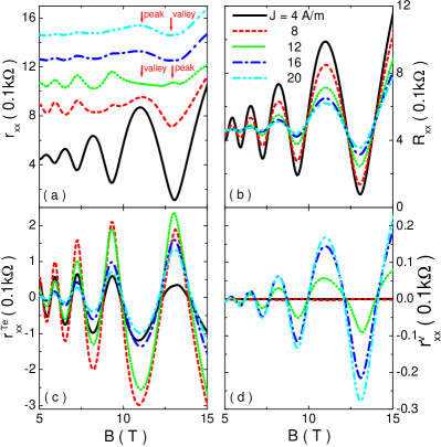
Figure 3: (Color online) Differential magnetoresistivity $r_{xx}$ (a), and its constituent parts $R_{xx}$ (b), $r_{xx}^{T_{\rm e}}$ (c) and $r_{xx}^{v}$ (d) defined in (27), are shown versus magnetic field for various bias current densities $J=4$, 8, 12, 16, 20$\,{\rm A/m}$. The $r_{xx}$ curves in (a) are vertically offset for clarity.

III.2 Current-induced magnetoresistance oscillation

We turn to the regime of lower magnetic fields, where the SdHO hardly shows up.

In the case of low temperature $T_{\rm e}\ll\varepsilon_{\rm F}$ and large filling factor $\nu=\tfrac{\pi N}{2eB}\gg 1$, the major contribution to the summation in the density correlation function (17) comes from Landau levels near the Fermi energy, i.e., terms $n\simeq n^{\prime}\sim\nu$, and then the function $C_{n,n^{\prime}}(x)$ has a sharp principal maximum near $x\sim 4\nu$. Therefore, as a function of the in-plane momentum ${q}$, the $\varPi_{2}(\bm{q},\omega)$ function given in (17) sharply peaks around $q\approx 2k_{\rm F}$, with $k_{\rm F}=\sqrt{\pi N}$ being the Fermi wave vector. In the case of a finite drift velocity $v$, the motion of the center-of-mass provides the relative electron with an additional energy $\omega_{0}={\bm{q}}\cdot{\bm{v}}$ during its transition from a state to another state having a momentum change of ${\bm{q}}$, as shown in the expressions of (9), (10) and (11) for $\bm{f}_{\rm i}$, $\bm{f}_{\rm p}$ and $w$. The sharp peaking of $\varPi_{2}(\bm{q},\omega)$ function around $q\approx 2k_{\rm F}$ indicates that most effective processes contributing to the magnetoresistance come from those electron transitions which involve an additional energy around $\omega_{j}=2k_{\rm F}v$. Looking at electron transitions in the Landau representation, we can see that the transition rate is proportional to the overlap of the DOS of the related two Landau levels around the Fermi surface, ${\rm Im}G_{n}(\epsilon+\omega_{j}){\rm Im}G_{n^{\prime}}(\epsilon)$, and the maximum overlap occurs at $\varepsilon_{n}-\varepsilon_{n^{\prime}}=\omega_{j}$. Thus, the impurity-induced longitudinal magnetoresistivity may show extrema when $\varepsilon_{\nu+l}-\varepsilon_{\nu}\approx l\omega_{\rm B}=\pm\omega_{j}$ with $l=0,\pm 1,\pm 2,...$ and $\omega_{\rm B}=eBv_{\rm F}/k_{\rm F}$ being the distance of the neighboring Landau levels in the vicinity of Fermi surface. Therefore, the impurity-related magnetoresistivity would exhibits a periodical oscillation when changing drift velocity $v$ or changing magnetic field $B$. This current-induced magnetoresistance oscillation (CIMO) is characterized by a dimensionless parameter $\omega_{j}/\omega_{\rm B}$ with a period $\Delta(\omega_{j}/\omega_{\rm B})\approx 1$: when $\omega_{j}/\omega_{\rm B}$ varies by a unity value, the magnetoresistivity experiences change of an oscillatory period.

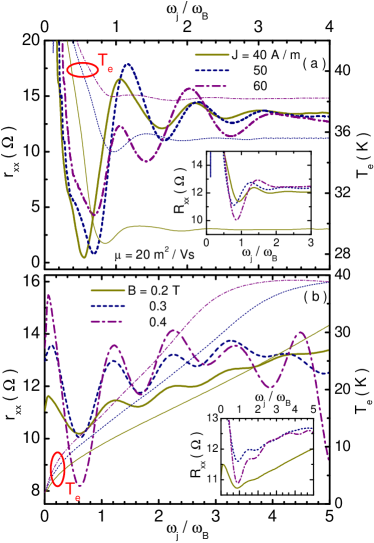
Figure 4: (Color online) Differential magnetoresistivity $r_{xx}$, electron temperature $T_{\rm e}$ and magnetoresistivity $R_{xx}$ (inset) are shown as functions of $\omega_{j}/\omega_{\rm B}$ for various fixed dc current densities $J=$40, 50, 60$\,{\rm A/m}$ (a) and for various fixed magnetic fields $B=0.2,0.3,0.4\,{\rm T}$ (b). The system is a suspended monolayer graphene having electron density $N=3.16\times 10^{12}\,{\rm cm^{-2}}$ and zero-magnetic-field mobility $\mu=20\,{\rm m^{2}/Vs}$ at lattice temperature $T=2\,{\rm K}$, with Coulombic impurity potential (24) of $d=0$.

As an example, Fig. 4 displays the calculated magnetoresistivity and differential magnetoresistivity versus $\omega_{j}/\omega_{\rm B}$ for fixed bias current densities $J=40,50$ and $60$ A/m (a) or for fixed magnetic fields $B=0.2,0.3$ and $0.4$ T (b) at lattice temperature $T=2$ K in a suspended monolayer graphene having electron density $N=3.16\times 10^{12}\,{\rm cm^{-2}}$ and linear mobility $\mu=20\,{\rm m^{2}/Vs}$, assuming Coulombic impurity scattering potential (24) with $d=0$. The longitudinal magnetoresistivity $R_{xx}$ (plotted in the insets) shows relatively weak oscillations, while the differential magnetoresistivity $r_{xx}$ exhibits marked oscillations, having an approximate period $\Delta(\omega_{j}/\omega_{\rm B})\approx 1$ in both cases. Notable magnetoresistance oscillations appear in the well-resolved Landau level regime when $2\varGamma\leq\omega_{\rm B}$, or $B\geq 8\alpha_{\Gamma}/\pi\mu\approx 0.25\,$T, and the enhanced current weakens the oscillation amplitude due to the rising electron temperature.

Note that the parameter $\omega_{j}/\omega_{\rm B}=(2\pi/e^{2}v_{\rm F})(J/B)$ characterizing the CIMO depends only on the band-dispersion related $v_{\rm F}$ for systems of linear energy band, thus the periodic behavior of CIMO is universal in graphene in terms of $J/B$, irrespective of carrier-density $N$. This situation is in contrast to the conventional 2DEG of parabolic band,lei2007current where the Fermi velocity $v_{\rm F}$ involved in the characterizing parameter depends on the carrier density, so does the periodicity of the magnetoresistance oscillation in it.

The basic features of the oscillatory $R_{xx}$ and $r_{xx}$ are: oscillation amplitude decays with increasing $\omega_{j}/\omega_{\rm B}$ but enhances with increasing current density or magnetic field strength in the discussed range. In the fixed current density case of Fig. 4(a), where the electron temperature has only weak change with changing magnetic field, the amplitude decrease of the resistance oscillation is due to the enlarged overlap of neighboring Landau levels with decreasing magnetic field. In the fixed $B$-field case of Fig. 4(b), the electron temperature grows when increasing bias current density, resulting in the suppression of the resistance oscillation. Nevertheless, the oscillation amplitude shown in these figures exhibits somewhat anomalous behavior, especially around the first peak of $J=60\,{\rm A/m}$ curve in Fig. 4(a) and the last peak of $B=0.4\,{\rm T}$ curve in Fig. 4(b). These $r_{xx}$ anomalies come from the contribution of phonon-related differential resistivity $r_{\rm ph}$.

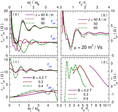
Figure 5: (Color online) Impurity-related and phonon-related differential resistivities $r_{\rm im}$ and $r_{\rm ph}$ are shown versus $\omega_{j}/\omega_{\rm B}$ for fixed current densities $J=40,50,60\,{\rm A/m}$ (a) or fixed magnetic fields $B=0.2,0.3,0.4\,{\rm T}$ (c). Phonon-related differential resistivity $r_{\rm ph}$ is replotted as a function of $\varepsilon_{p}-\varepsilon_{j}$ for fixed current densities (b) or fixed magnetic fields (d).

In contrast to the case of high-mobility 2DEG,lei2007current the electron temperature $T_{\rm e}$ in the present monolayer graphene may reach the range of 40 K in the case of high current density $J\geq 60$ A/m and the magnitude of phonon-related resistivity may not be negligible in comparison with impurity contribution as shown in Fig. 5(a) and (c), where the constituent parts of $r_{xx}$ in the monolayer graphene, the resistivity $r_{\rm im}=-(N^{2}e^{2})^{-1}df_{\rm i}/dv$ due to impurity scattering and the resistivity $r_{\rm ph}=-(N^{2}e^{2})^{-1}df_{\rm p}/dv$ due to intrinsic acoustic phonon scattering, are plotted as functions of $\omega_{j}/\omega_{\rm B}$ respectively for the cases of fixed current density (a) and for the cases of fixed magnetic field strength (c). The oscillation behavior of $r_{\rm im}$ closely follows the basic feature of CIMO, but $r_{\rm ph}$, though generally smaller in magnitude, appears quite different. In the fixed current case the marked drop of $r_{\rm ph}$ around $\omega_{j}/\omega_{\rm B}\sim 1$ [Fig. 5(a)] leads to the descent of the first peak of $r_{xx}$ at $J=60\,{\rm A/m}$ curve in Fig. 4(a). In the fixed magnetic field case, the resonant peak of $r_{\rm ph}$ around $\omega_{j}/\omega_{\rm B}\sim 4.5$ for $B=0.4\,{\rm T}$ [Fig. 5(c)] gives rise to the enhancement and position shift of the last peak of $r_{xx}$ in Fig. 4(b).

Such kind of oscillatory $r_{\rm ph}$ is referred to the magnetophonon resonance induced by acoustic phonons. As in conventional 2DEGs,Zudov2001new ; zhang2008resonant ; lei2008low acoustic phonon-related resistivity $r_{\rm ph}$ in a dc biased graphene should feature a periodical appearance of resonant peaks with respect to $\varepsilon_{p}-\varepsilon_{j}$ axis, where $\varepsilon_{j}\equiv\omega_{j}/\omega_{\rm B}$ and $\varepsilon_{p}\equiv\omega_{\rm ph}/\omega_{\rm B}$ are the ratios of the energy $\omega_{j}$ provided by the drifting center-of-mass and the energy $\omega_{\rm ph}=2k_{\rm F}v_{\rm ph}$ provided by the optimum phonons to the inter-Landau-level distance $\omega_{\rm B}$ of electron near the Fermi surface. We replot the phonon-related resistivities $r_{\rm ph}$ given in Fig. 5(a) and (c) as a function of $\varepsilon_{p}-\varepsilon_{j}$ in Fig. 5(b) and (d). They indeed show peaks near integer positions $\varepsilon_{p}-\varepsilon_{j}\approx l=1,2,3$ and $4$, indicating electron scattered resonantly across $l$ Landau-level spacings by absorbing or emitting an optimum acoustic phonon under the biased dc current condition. At low magnetic fields, the magnetophonon resonance in $r_{\rm ph}$ can not be seen in the range shown, because of weakened oscillation in the DOS and higher orders of resonant peaks required (e.g., $\varepsilon_{p}-\varepsilon_{j}\geq 6$ for $0\leq\varepsilon_{j}\leq 5$ at $B=0.2\,{\rm T}$ ).

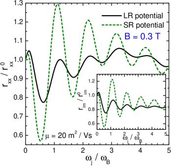
Figure 6: (Color online) Normalized differential resistivity versus $\omega_{j}/\omega_{\rm B}$ at fixed magnetic field $B=0.3\,{\rm T}$ for the system subject to LR or SR impurity-scattering. The inset displays normalized impurity-related differential resistivity $r_{\rm im}$. Here $r_{xx}^{0}$ and $r_{\rm im}^{0}$ are total and impurity-related differential resistivity in the absence of magnetic field. The zero-magnetic-field mobility $\mu=20\,{\rm m^{2}/Vs}$.

Analogous to the case of 2DEG,lei2003radiation ; lei2010mater the amplitude of current-controlled magnetoresistance oscillation depends strongly on the correlation length of electron-impurity scattering potential, though the oscillation periods are essentially the same in terms of $\varepsilon_{j}$. To see this, we plot the normalized total and impurity-induced differential resistivities, $r_{xx}$ and $r_{\rm im}$, for Coulombic impurity scattering potential (24) with $d=0$ (LR) and short-range (SR) disorders (assuming same zero-magnetic-field mobility $\mu=20\,{\rm m^{2}/Vs}$ and $\alpha_{\Gamma}=2$ for both cases) in Fig. 6 as functions of $\omega_{j}/\omega_{\rm B}$ at fixed magnetic field $B=0.3\,{\rm T}$. The lattice defects in graphene are usually modeled by SR impurities. It is seen that both $r_{xx}$ and $r_{\rm im}$ display much stronger oscillations in the case of SR potential than that of LR potential, but the maxima and minima positions are almost identical in both cases.

IV summary

In summary, we have presented an investigation of nonlinear magnetotransport in graphene under a finite dc bias at low temperature employing a balance-equation scheme appropriate to systems with linear-energy dispersion. In the relatively strong magnetic field range when SdHO controlled by the filling factor $\nu=2\pi N/eB$ shows up we find that the oscillatory differential magnetoresistivity exhibits phase inversion with rising bias current density, in agreement with recent experimental finding. Further, it is demonstrated that electron–SO-phonon scattering is important for graphene on a polar substrate, which suppresses the rapid increase of electron temperature and may result in a second phase inversion of the oscillatory resistance. In the lower magnetic field and higher bias current density regime when SdHO becomes weak a CIMO is appreciable in suspended graphene. It appears markedly in the differential resistivity when Landau levels are still well resolved and is controlled by the parameter $\varepsilon_{j}=(2\pi/e^{2}v_{\rm F})(J/B)$ having approximate period $\Delta\varepsilon_{j}\sim 1$. For the graphene mobility available today ($\approx 20\,{\rm m^{2}/Vs}$), the oscillatory behavior may be some what altered by magnetophonon resonance induced by intrinsic acoustic phonon under finite bias current. We hope this current-controlled magnetoresistance oscillation could be observed experimentally in the near future.

Appendix: Derivation of the energy-balance equation

Here we detail the derivation of the energy-balance equation for graphene. In the second quantization representation of the creation (annihilation) operators $c_{\alpha\lambda nk_{x}s}^{{\dagger}}$ ($c_{\alpha\lambda nk_{x}s}$), the relative-carrier Hamiltonian has the form:

$$\mathcal{H}_{\rm er}=\sum_{\alpha,\lambda,n,k_{x},s}\varepsilon_{\lambda n}c_{\alpha\lambda nk_{x}s}^{{\dagger}}c_{\alpha\lambda nk_{x}s}$$ (28)

The rate of change of the energy of relative carrier system is obtained from the Heisenberg equation of motion:

$$\dot{\mathcal{H}}_{\rm er}= -i[\mathcal{H}_{\rm er},\mathcal{H}]$$

$$= -\sum_{\bm{q},a}U(\bm{q},z_{a})e^{i\bm{q}\cdot(\bm{R}-\bm{r}_{a})}\frac{d\rho_{\bm{q}}(t)}{dt}$$

$$-\sum_{\bm{q},\nu}M(\bm{q},\nu)e^{i\bm{q}\cdot\bm{R}}\varphi_{\bm{q}\nu}(t)\frac{d\rho_{\bm{q}}(t)}{dt}.$$ (29)

Here the particle density operator

$$\rho_{\bm{q}}(t)=\sum_{\begin{subarray}{c}\alpha,s,\lambda,n,k_{x}\\ \alpha^{\prime},s^{\prime},\lambda^{\prime},n^{\prime},k_{x}^{\prime}\end{subarray}} \langle\Psi_{nk_{x}s}^{\alpha\lambda}|e^{i\bm{q}\cdot\bm{r}}|\Psi_{n^{\prime}k_{x}^{\prime}s^{\prime}}^{\alpha^{\prime}\lambda^{\prime}}\rangle e^{i(\varepsilon_{\lambda n}-\varepsilon_{\lambda^{\prime}n^{\prime}})t}$$

$$\times c_{\alpha\lambda nk_{x}s}^{{\dagger}}c_{\alpha^{\prime}\lambda^{\prime}n^{\prime}k_{x}^{\prime}s^{\prime}}$$ (30)

After statistical average of the operator equation (Appendix: Derivation of the energy-balance equation), the energy-balance equation is given bylei2008balance

$$\frac{dU}{dt}=\left\langle\frac{d\mathcal{H}_{\rm er}}{dt}\right\rangle=I_{1}+I_{2},$$ (31)

with

$$I_{1}=i\int_{-\infty}^{t}dt^{\prime}n_{\rm i}\sum_{\bm{q}} |U(\bm{q})|^{2}e^{i\bm{q}\cdot[\bm{R}(t)-\bm{R}(t^{\prime})]}$$

$$\times\left\langle\left[\frac{d\rho_{\bm{q}}(t)}{dt},\rho_{-\bm{q}}(t^{\prime})\right]\right\rangle_{0},$$ (32)

$$I_{2}=i\int_{-\infty}^{t}dt^{\prime}\sum_{\bm{q},\nu} |M(\bm{q},\nu)|^{2}e^{i\bm{q}\cdot[\bm{R}(t)-\bm{R}(t^{\prime})]}$$

$$\times\left\langle\left[\varphi_{\bm{q}\nu}(t)\frac{d\rho_{\bm{q}}(t)}{dt},\varphi_{-\bm{q}\nu}(t^{\prime})\rho_{-\bm{q}}(t^{\prime})\right]\right\rangle_{0}.$$ (33)

The first integral $I_{1}$ can be simplified as

$$I_{1}= -\int_{-\infty}^{\infty}dt^{\prime}n_{\rm i}\sum_{\bm{q}}|U(\bm{q})|^{2}e^{i\bm{q}\cdot\bm{v}(t-t^{\prime})}\frac{d}{dt}\varPi(\bm{q},t-t^{\prime})$$

$$-i\sum_{\bm{q}}|U(\bm{q})|^{2}\left\langle\left[\rho_{\bm{q}}(t),\rho_{-\bm{q}}(t)\right]\right\rangle_{0}.$$ (34)

Here the relative-carrier density correlation function $\varPi(\bm{q},t-t^{\prime})=-i\theta(t-t^{\prime})\left\langle\left[\rho_{\bm{q}}(t),\rho_{-\bm{q}}(t^{\prime})\right]\right\rangle_{0}$. The second term of the above equation equals zero and the first term becomes $-\bm{f}_{\rm i}\cdot\bm{v}$ after integration by parts, hence we obtain $I_{1}=-\bm{f}_{\rm i}\cdot\bm{v}$. Similarly, the integral $I_{2}=-\bm{f}_{\rm p}\cdot\bm{v}-w$. Therefore, the energy-balance equation is written as

$$\frac{dU}{dt}=\left\langle\frac{d\mathcal{H}_{\rm er}}{dt}\right\rangle=-(\bm{f}_{\rm i}+\bm{f}_{\rm p})\cdot\bm{v}-w.$$ (35)

References

- (1) K. S. Novoselov, A. K. Geim, S. V. Morozov, D. Jiang, Y. Zhang, S. V. Dubonos, I. V. Grigorieva, and A. A. Firsov, Science 306, 666 (2004).
- (2) A. K. Geim and K. S. Novoselov, Nat. Mat. 6, 183 (2007).
- (3) S. D. Sarma, S. Adam, E. H. Hwang, and E. Rossi, Rev. Mod. Phys. 83, 407 (2011).
- (4) M. O. Goerbig, Rev. Mod. Phys. 83, 1193 (2011).
- (5) Y. Zhang, Y. Tan, H. Stormer, and P. Kim, Nature 438, 201 (2005).
- (6) K. S. Novoselov, A. K. Geim, S. V. Morozov, D. Jiang, M. I. Katsnelson, I. V. Grigorieva, S. V. Dubonos, and A. A. Firsov, Nature 438, 197 (2005).
- (7) Z. Tan, C. Tan, L. Ma, G. T. Liu, L. Lu, and C. L. Yang, Phys. Rev. B 84, 115429 (2011).
- (8) S. Fratini and F. Guinea, Phys. Rev. B 77, 195415 (2008).
- (9) X. Li, E. A. Barry, J. M. Zavada, M. B. Nardelli, and K. W. Kim, Appl. Phys. Lett. 97, 082101 (2010).
- (10) W. Zhu, V. Perebeinos, M. Freitag, and P. Avouris, Phys. Rev. B 80, 235402 (2009).
- (11) N. R. Kalmanovitz, A. A. Bykov, S. Vitkalov, and A. I. Toropov, Phys. Rev. B 78, 085306 (2008).
- (12) C. L. Yang, J. Zhang, R. R. Du, J. A. Simmons, and J. L. Reno, Phys. Rev. Lett. 89, 076801 (2002).
- (13) A. A. Bykov, J. Q. Zhang, S. Vitkalov, A. K. Kalagin, and A. K. Bakarov, Phys. Rev. B 72, 245307 (2005).
- (14) W. Zhang, H. S. Chiang, M. A. Zudov, L. N. Pfeiffer, and K. W. West, Phys. Rev. B 75, 041304 (2007).
- (15) X. L. Lei, Appl. Phys. Lett. 90, 132119 (2007).
- (16) J. Q. Zhang, S. Vitkalov, A. A. Bykov, A. K. Kalagin, and A. K. Bakarov, Phys. Rev. B 75, 081305 (2007).
- (17) M. G. Vavilov, I. L. Aleiner, and L. I. Glazman, Phys. Rev. B 76, 115331 (2007).
- (18) K. I. Bolotin, K. J. Sikes, Z. Jiang, M. Klima, G. Fudenberg, J. Hone, P. Kim, and H. L. Stormer, Solid State Commun. 146, 351 (2008).
- (19) K. I. Bolotin, K. J. Sikes, J. Hone, H. L. Stormer, and P. Kim, Phys. Rev. Lett. 101, 096802 (2008).
- (20) X. L. Lei and C. S. Ting, Phys. Rev. B 32, 1112 (1985).
- (21) X. L. Lei, J. L. Birman, and C. S. Ting, J. Appl. Phys. 58, 2270 (1985).
- (22) W. Cai, X. L. Lei, and C. S. Ting, Phys. Rev. B 31, 4070 (1985).
- (23) X. L. Lei, D. Y. Xing, M. Liu, C. S. Ting, and J. L. Birman, Phys. Rev. B 36, 9134 (1987).
- (24) X. L. Lei, Balance equation approach to electron transport in semiconductors (World Scientific, Singapore, 2008).
- (25) C. M. Wang and X. L. Lei, Phys. Rev. B 86, 035442 (2012).
- (26) C. S. Ting, S. C. Ying, and J. J. Quinn, Phys. Rev. B 16, 5394 (1977).
- (27) R. Roldán, J.-N. Fuchs, and M. O. Goerbig, Phys. Rev. B 80, 085408 (2009).
- (28) P. K. Pyatkovskiy and V. P. Gusynin, Phys. Rev. B 83, 075422 (2011).
- (29) T. Ando, A. B. Fowler, and F. Stern, Rev. Mod. Phys. 54, 437 (1982).
- (30) Y. Zheng and T. Ando, Phys. Rev. B 65, 245420 (2002).
- (31) X. L. Lei and S. Y. Liu, Phys. Rev. Lett. 91, 226805 (2003); Phys. Rev. B, 72, 075345 (2005).
- (32) E. H. Hwang, S. Adam, and S. Das Sarma, Phys. Rev. Lett. 98, 186806 (2007).
- (33) C. M. Wang and F. J. Yu, Phys. Rev. B 84, 155440 (2011).
- (34) A. Konar, T. Fang, and D. Jena, Phys. Rev. B 82, 115452 (2010).
- (35) Massimo V. Fischetti, Deborah A. Neumayer, and E. A. Cartier, J. Appl. Phys. 90, 4587 (2001).
- (36) V. Perebeinos and P. Avouris, Phys. Rev. B 81, 195442 (2010).
- (37) R. Kim, V. Perebeinos, and P. Avouris, Phys. Rev. B 84, 075449 (2011).
- (38) E. H. Hwang and S. Das Sarma, Phys. Rev. B 77, 115449 (2008).
- (39) J. Chen, C. Jang, S. Xiao, M. Ishigami, and M. Fuhrer, Nat. Nanotechnol. 3, 206 (2008).
- (40) M. A. Zudov, I. V. Ponomarev, A. L. Efros, R. R. Du, J. A. Simmons, and J. L. Reno, Phys. Rev. Lett. 86, 3614 (2001).
- (41) W. Zhang, M. A. Zudov, L. N. Pfeiffer, and K. W. West, Phys. Rev. Lett. 100, 036805 (2008).
- (42) X. L. Lei, Phys. Rev. B 77, 205309 (2008).
- (43) X. L. Lei, Mater. Sci. Eng. R, 70, 126 (2010).