Efficient Transmit Beamspace Design for Search-free Based DOA Estimation in
MIMO Radar

Abstract

In this paper, we address the problem of transmit beamspace design for multiple-input multiple-output (MIMO) radar with colocated antennas in application to direction-of-arrival (DOA) estimation. A new method for designing the transmit beamspace matrix that enables the use of search-free DOA estimation techniques at the receiver is introduced. The essence of the proposed method is to design the transmit beamspace matrix based on minimizing the difference between a desired transmit beampattern and the actual one under the constraint of uniform power distribution across the transmit array elements. The desired transmit beampattern can be of arbitrary shape and is allowed to consist of one or more spatial sectors. The number of transmit waveforms is even but otherwise arbitrary. To allow for simple search-free DOA estimation algorithms at the receive array, the rotational invariance property is established at the transmit array by imposing a specific structure on the beamspace matrix. Semidefinite relaxation is used to transform the proposed formulation into a convex problem that can be solved efficiently. We also propose a spatial-division based design (SDD) by dividing the spatial domain into several subsectors and assigning a subset of the transmit beams to each subsector. The transmit beams associated with each subsector are designed separately. Simulation results demonstrate the improvement in the DOA estimation performance offered by using the proposed joint and SDD transmit beamspace design methods as compared to the traditional MIMO radar technique.

I Introduction

In array processing applications, the direction-of-arrival (DOA) parameter estimation problem is the most fundamental one [1]. Many DOA estimation techniques have been developed for the classical array processing single-input multiple-output (SIMO) setup [1], [2]. The development of a novel array processing configuration that is best known as multiple-input multiple-output (MIMO) radar [3], [4] has opened new opportunities in parameter estimation. Many works have recently been reported in the literature showing the benefits of applying the MIMO radar concept using widely separated antennas [5]–[8] as well as using colocated transmit and receive antennas [9]–[16]. We focus on the latter case in this paper.

In MIMO radar with colocated antennas, a virtual array with a larger number of virtual antenna elements can be formed and used for improved DOA estimation performance as compared to the performance of SIMO radar [17], [18] for relatively high signal-to-noise ratios (SNRs), i.e., when the benefits of increased virtual aperture start to show up. The SNR gain for the traditional MIMO radar (with the number of waveforms being the same as the number of transmit antenna elements), however, decreases as compared to the phased-array radar where the transmit array radiates a single waveform coherently from all antenna elements [12], [13]. A trade-off between the phased-array and the traditional MIMO radar can be achieved [12], [14], [19] which gives the best of both configurations, i.e., the increased number of virtual antenna elements due to the use of waveform diversity together with SNR gain due to subaperture based coherent transmission.

Several transmit beamforming techniques have been developed in the literature to achieve transmit coherent gain in MIMO radar under the assumption that the general angular locations of the targets are known a priori to be located within a certain spatial sector. The increased number of degrees of freedom for MIMO radar, due to the use of multiple waveforms, is used for the purpose of synthesizing a desired transmit beampattern based on optimizing the correlation matrix of the transmitted waveforms [4], [20], [21]. To apply the designs obtained using the aforementioned methods, the actual waveforms still have to be found which can be a difficult and computationally demanding problem [22].

One of the major motivations for designing transmit beampattern is realizing the possibility of achieving SNR gain together with increased aperture for improved DOA estimation in a wide range of SNRs [15], [23]. In particular, it has been shown in [15] that the performance of a MIMO radar system with a number of waveforms less than the number of transmit antennas and with transmit beamspace design capability is better than the performance of a MIMO radar system with full waveform diversity and no transmit beamforming gain. Remarkably, using MIMO radar with proper transmit beamspace design, it is possible to guarantee the satisfaction of such desired property for DOA estimation as the rotational invariance property (RIP) at the receive array [15]. This is somewhat similar in effect to the property of orthogonal space-time block codes in that the shape of the transmitted constellation does not change at the receiver independent of the channel. The latter allows for simple decoder [24]. Similarly, here the RIP allows for simple DOA estimation techniques at the receiver although the RIP is actually enforced at the transmitter, and the propagation media cannot break it thanks to the proper design of transmit beamspace. Since the RIP holds at the receive array independent of the propagation media and receive antenna array configuration, the receive antenna array can be any arbitrary array. However, the methods developed in [15] suffer from the shortcomings that the transmit power distribution across the array elements is not uniform and the achieved phase rotations come with variations in the magnitude of different transmit beams that affects the performance of DOA estimation at the receiver.

In this paper, we consider the problem of transmit beamspace design for DOA estimation in MIMO radar with colocated antennas. We propose a new method for designing the transmit beamspace that enables the use of search-free DOA estimation techniques at the receive antenna array. The essence of the proposed method is to design the transmit beamspace matrix based on minimizing the difference between a desired transmit beampattern and the actual one while enforcing the uniform power distribution constraint across the transmit array antenna elements. The desired transmit beampattern can be of arbitrary shape and is allowed to consist of one or more spatial sectors. The case of even but otherwise arbitrary number of transmit waveforms is considered. To allow for simple search-free DOA estimation algorithms at the receiver, the RIP is established at the transmit antenna array by imposing a specific structure on the transmit beamspace matrix. The proposed structure is based on designing the transmit beams in pairs where the transmit weight vector associated with a certain transmit beam is the conjugate flipped version of the weight vector associated with another beam, i.e., one transmit weight vector is designed for each pair of transmit beams. All pairs are designed jointly while satisfying the requirement that the two transmit beams associated with each pair enjoy rotational invariance with respect to each other. Semidefinite programming (SDP) relaxation is used to transform the proposed formulation into a convex problem that can be solved efficiently using, for example, interior point methods. In comparison to our previous method [23] that achieves phase rotation between two transmit beams, the proposed method enjoys the following advantages. (i) It ensures that the magnitude response of the two transmit beams associated with one pair of transmit beams is exactly the same at all spatial directions, a property that improves the DOA estimation performance. (ii) It ensures uniform power distribution across transmit elements. (iii) It enables estimating the DOAs via estimating the accumulated phase rotations over all transmit beams instead of only two beams. (iv) It only involves optimization over half the entries of the transmit beamspace matrix which decreases the computational load. We also propose an alternative formulation based on splitting the overall transmit beamspace design problem into several smaller problems. The alternative formulation is referred to as the spatial-division based design (SDD) which involves dividing the spatial domain into several subsectors and assigning a subset of the transmit beamspace pairs to each subsector. The SDD method enables post processing of data associated with different subsectors independently with estimation performance comparable to the performance of the joint transmit beamspace design. Simulation results demonstrate the improvement in the DOA estimation performance that is achieved by using the proposed joint transmit beamspace design and SDD methods as compared to the traditional MIMO radar technique.

The rest of the paper is organized as follows. Section II introduces the system model for mono-static MIMO radar system with transmit beamspace. The problem formulation is developed in Section III while the transmit beamspace design problem for even but otherwise arbitrary number of transmit waveforms is developed in Section IV. Section V gives simulation examples for the proposed DOA estimation techniques and conclusions are drawn in Section VI.

II System Model and Main Idea

Consider a mono-static MIMO radar system equipped with a uniform linear transmit array of $M$ colocated antennas with inter-element spacing $d$ measured in wavelength and a receive array of $N$ antennas configured in a random shape. The transmit and receive arrays are assumed to be close enough to each other such that the spatial angle of a target in the far-field remains the same with respect to both arrays. Let ${\boldsymbol{\Phi}}(t)=[\phi_{1}(t),\ldots,\phi_{K}(t)]^{T}$ be the $K\times 1$ vector that contains the complex envelopes of the waveforms $\phi_{k}(t),\ k=1,\ldots,K$ which are assumed to be orthogonal, i.e.,

$$\int_{0}^{\rm T_{p}}{\phi_{i}(t)\phi_{j}^{*}}(t)=\delta(i-j),\qquad i,j=1,2,\cdots,K$$ (1)

where $T_{p}$ is the pulse duration, $(\cdot)^{T}$ and $(\cdot)^{*}$ stand for the transpose and the conjugate, respectively, and $\delta(\cdot)$ is the Kroneker delta. The actual transmitted signals are taken as linear combinations of the orthogonal waveforms. Therefore, the $M\times 1$ vector of the baseband representation of the transmitted signals can be written as [15]

$$\mathbf{s}(t)=\left[s_{1}(t),\ldots,s_{M}(t)\right]^{T}=\mathbf{W}{\boldsymbol{\Phi}}(t)$$ (2)

where $s_{i}(t)$ is the signal transmitted from antenna $i$ and

$$\mathbf{W}=\begin{pmatrix}w_{1,1}&w_{2,1}&\cdots&w_{K,1}\\ w_{1,2}&w_{2,2}&\cdots&w_{K,2}\\ \vdots&\vdots&\ddots&\vdots\\ w_{1,M}&w_{2,M}&\cdots&w_{K,M}\end{pmatrix}$$ (3)

is the $M\times K$ transmit beamspace matrix. It is worth noting that each of the orthogonal waveforms $\phi_{k}(t),\ k=1,\ldots,K$ is transmitted over one transmit beam where the $k$th column of the matrix $\mathbf{W}$ corresponds to the transmit beamforming weight vector used to form the $k$th beam.

Let $\mathbf{a}(\theta)\triangleq[1,e^{-j2\pi d\sin(\theta)},\ldots,e^{-j2\pi d(M-1)\sin(\theta)}]^{T}$ be the $M\times 1$ transmit array steering vector. The transmit power distribution pattern can be expressed as [20]

$$G(\theta)=\frac{1}{4\pi}\mathbf{d}^{H}(\theta)\mathbf{R}\mathbf{d}(\theta),\quad-\pi/2\leq\theta\leq\pi/2$$ (4)

where $(\cdot)^{H}$ stands for the conjugate transpose, $\mathbf{d}(\theta)=$ $\mathbf{a}^{*}(\theta)$, and

$${\bf R}=\int_{0}^{\rm T_{p}}{\bf s}(t){\bf s}^{H}(t)dt$$ (5)

is the cross-correlation matrix of the transmitted signals (2). One way to achieve a certain desired transmit beampattern is to optimize over the cross-correlation matrix ${\bf R}$ such as in [20], [21]. In this case, a complementary problem has to be solved after obtaining ${\bf R}$ in order to find appropriate signal vector ${\bf s}(t)$ that satisfies (5). Solving such a complementary problem is in general difficult and computationally demanding. However, in this paper, we extend our approach of optimizing the transmit beampattern via designing the transmit beamspace matrix. According to this approach, the cross-correlation matrix is expressed as

$$\mathbf{R}=\mathbf{W}\mathbf{W}^{H}$$ (6)

that holds due to the orthogonality of the waveforms (see (1) and (2)). Then the transmit beamspace matrix $\mathbf{W}$ can be designed to achieve the desired beampattern while satisfying many other requirements mandated by practical considerations such as equal transmit power distribution across the transmit array antenna elements, achieving a desired radar ambiguity function, etc. Moreover, this approach enables enforcing the RIP which facilitates subsequent processing steps at the receive antenna array, e.g., it enables applying accurate computationally efficient DOA estimation using search-free direction finding techniques such as ESPRIT.

The signal measured at the output of the receive array due to echoes from $L$ narrowband far-field targets can be modeled as

$$\mathbf{x}(t,\tau)=\sum_{l=1}^{L}\beta_{l}(\tau)\left[\mathbf{d}^{H}(\theta_{l})\mathbf{W}{\boldsymbol{\Phi}}(t)\right]\mathbf{b}(\theta_{l})+\mathbf{z}(t,\tau)$$ (7)

where $t$ is the time index within the radar pulse, $\tau$ is the slow time index , i.e., the pulse number, $\beta_{l}(\tau)$ is the reflection coefficient of the target located at the unknown spatial angle $\theta_{l}$, $\mathbf{b}(\theta_{l})$ is the receive array steering vector, and $\mathbf{z}(t,\tau)$ is the $N\times 1$ vector of zero-mean white Gaussian noise with variance $\sigma_{z}^{2}$. In (7), the target reflection coefficients $\beta_{l}(\tau),\ l=1,\ldots,L$ are assumed to obey the Swerling II model, i.e, they remain constant during the duration of one radar pulse but change from pulse to pulse. Moreover, they are assumed to be drawn from a normal distribution with zero mean and variance $\sigma_{\beta}^{2}$.

By matched filtering $\mathbf{x}(t,\tau)$ to each of the orthogonal basis waveforms $\phi_{k}(t),k=1,\ldots,K$, the $N\times 1$ virtual data vectors can be obtained as

$$\!\!\!\mathbf{y}_{k}(\tau)\! \!\!\!=\!\!\! \!\int_{\rm T_{p}}\mathbf{x}(t,\tau)\phi_{k}^{*}(t)dt$$ (8)

$$\!\!\!=\!\!\! \!\sum_{l=1}^{L}\beta_{l}(\tau)\left({\mathbf{d}}^{H}(\theta_{l}){\mathbf{w}}_{k}\right)\mathbf{b}(\theta_{l})+{\mathbf{z}}_{k}(\tau)$$

where ${\mathbf{w}}_{k}$ is the $k$th column of the transmit beamspace matrix $\mathbf{W}$ and ${\mathbf{z}}_{k}(\tau)\triangleq\int_{\rm T_{\rm p}}\mathbf{z}(t,\tau)\phi_{k}^{*}(t)dt$ is the $N\times 1$ noise term whose covariance is $\sigma_{z}^{2}\mathbf{I}_{N}$.

Let $\breve{\mathbf{y}}_{l,k}(\tau)$ be the noise free component of the virtual data vector (8) associated with the $l$th target, i.e., $\breve{\mathbf{y}}_{l,k}(\tau)=\beta_{l}(\tau)\left({\mathbf{d}}^{H}(\theta_{l}){\mathbf{w}}_{k}\right)\mathbf{b}(\theta_{l})$. Then, one can easily observe that the $k$th and the $k^{\prime}$th components associated with the $l$th target are related to each other through the following relationship

$$\breve{\mathbf{y}}_{l,k^{\prime}}(\tau)\! \!\!\!=\!\!\! \!\beta_{l}(\tau)\left({\mathbf{d}}^{H}(\theta_{l}){\mathbf{w}}_{k^{\prime}}\right)\mathbf{b}(\theta_{l})$$ (9)

$$\!\!\!=\!\!\! \!\frac{{\mathbf{d}}^{H}(\theta_{l}){\mathbf{w}}_{k^{\prime}}}{{\mathbf{d}}^{H}(\theta_{l}){\mathbf{w}}_{k}}\cdot\breve{\mathbf{y}}_{l,k}(\tau)$$

$$\!\!\!=\!\!\! \!e^{j\left(\psi_{k^{\prime}}(\theta_{l})-\psi_{k}(\theta_{l})\right)}\frac{\left|{\mathbf{d}}^{H}(\theta_{l}){\mathbf{w}}_{k^{\prime}}\right|}{\left|{\mathbf{d}}^{H}(\theta_{l}){\mathbf{w}}_{k}\right|}\cdot\breve{\mathbf{y}}_{l,k}(\tau)$$

where $\psi_{k}(\theta)$ is the phase of the inner product ${{\mathbf{d}}^{H}(\theta)\mathbf{w}}_{k}$. The expression (9) means that the signal component $y_{k}(\tau)$ corresponding to a given target is the same as the signal component $\mathbf{y}_{k^{\prime}}$ corresponding to the same target up to a phase rotation and a gain factor.

The RIP can be enforced by imposing the constraint $|{\mathbf{d}}^{H}(\theta){\mathbf{w}}_{k}|=|{\mathbf{d}}^{H}(\theta){\mathbf{w}}_{k^{\prime}}|$ while designing the transmit beamspace matrix $\mathbf{W}$. The main advantage of enforcing the RIP is that it allows us to estimate DOAs via estimating the phase rotation associated with the $k$th and $k^{\prime}$th pair of the virtual data vectors using search-free techniques, e.g., ESPRIT. Moreover, if the number of transmit waveforms is more than two, the DOA estimation can be carried out via estimating the phase difference

$$\angle\sum_{i=1}^{K/2}{\mathbf{d}}^{H}(\theta_{l})\mathbf{w}_{i}-\!\angle\!\!\!\sum_{i=K/2+1}^{K}\!\!\!{\mathbf{d}}^{H}(\theta_{l})\mathbf{w}_{i}$$ (10)

and comparing it to a precalculated phase profile for the given spatial sector in which we have concentrated power from the transmit antenna array. However, in the latter case, precautions should be taken to assure the coherent accumulation of the $K/2$ components in (10), i.e., to avoid gain loss as will be shown later in the paper.

III Problem formulation

The main goal is to design a transmit beamspace matrix $\mathbf{W}$ which achieves a spatial beampattern that is as close as possible to a certain desired one. Substituting (6) in (4), the spatial beampattern can be rewritten as

$$G(\theta) \!\!\!=\!\!\! \frac{1}{4\pi}\mathbf{d}^{H}(\theta)\mathbf{W}\mathbf{W}^{H}\mathbf{d}(\theta)$$ (11)

$$\!\!\!=\!\!\! \frac{1}{4\pi}\sum_{i=1}^{K}\mathbf{w}_{i}^{H}\mathbf{d}(\theta)\mathbf{d}^{H}(\theta)\mathbf{w}_{i}.$$

Therefore, we design the transmit beamspace matrix $\mathbf{W}$ based on minimizing the difference between the desired beampattern and the actual beampattern given by (11). Using the minmax criterion, the transmit beamspace matrix design problem can be formulated as

$$\!\!\!\min_{\mathbf{W}}\max_{\theta}\left|G_{\rm d}(\theta)-\frac{1}{4\pi}\sum_{i=1}^{K}\mathbf{w}_{i}^{H}\mathbf{d}(\theta)\mathbf{d}^{H}(\theta)\mathbf{w}_{i}\right|$$ (12)

$$\!\!\!{\rm s.t.}\ \ \ \sum_{i=1}^{K}|\mathbf{w}_{i}(j)|^{2}=\frac{P_{\rm t}}{M},\quad j=1,\cdots,M$$ (13)

where $G_{\rm d}(\theta),\theta\in[-\pi/2,\pi/2]$ is the desired beampattern and $P_{\rm t}$ is the total transmit power. The $M$ constraints enforced in (13) are used to ensure that individual antennas transmit equal powers given by $P_{\rm t}/M$. It is equivalent to having the norms of the rows of ${\mathbf{W}}$ to be equal to $P_{\rm t}/M$. The uniform power distribution across the array antenna elements given by (13) is necessary from a practical point of view. In practice, each antenna in the transmit array typically uses the same power amplifier, and thus has the same dynamic power range. If the power used by different antenna elements is allowed to vary widely, this can severely degrade the performance of the system due to the nonlinear characteristics of the power amplifier.

Another goal that we wish to achieve is to enforce the RIP to enable for search-free DOA estimation. Enforcing the RIP between the $k$th and $(K/2+k)$th transmit beams is equivalent to ensuring that the following relationship holds

$$\left|{\mathbf{w}}_{k}^{H}{\mathbf{d}}(\theta)\right|=\left|{\mathbf{w}}_{\frac{K}{2}+k}^{H}{\mathbf{d}}(\theta)\right|,\quad\theta\in[-\pi/2,\pi/2].$$ (14)

Ensuring (14), the optimization problem (12)–(13) can be reformulated as

$$\!\!\!\min_{\mathbf{W}}\max_{\theta}\left|G_{\rm d}(\theta)-\frac{1}{4\pi}\sum_{i=1}^{K}\mathbf{w}_{i}^{H}\mathbf{d}(\theta)\mathbf{d}^{H}(\theta)\mathbf{w}_{i}\right|$$ (15)

$$\!\!\!{\rm s.t.}\ \ \ \sum_{i=1}^{K}|\mathbf{w}_{i}(j)|^{2}=\frac{P_{\rm t}}{M},\quad j=1,\cdots,M$$ (16)

$$\!\!\!\qquad\ \ \ \left|{\mathbf{w}}_{k}^{H}{\mathbf{d}}(\theta)\right|=\left|{\mathbf{w}}_{\frac{K}{2}+k}^{H}{\mathbf{d}}(\theta)\right|,$$ (17)

$$\!\!\!\qquad\ \ \ \theta\in[-\pi/2,\pi/2],\quad k=1,\ldots,\frac{K}{2}.$$

It is worth noting that the constraints (16) as well as the constraints (17) correspond to non-convex sets and, therefore, the optimization problem (15)–(17) is a non-convex problem which is difficult to solve in a computationally efficient manner. Moreover, the fact that (17) should be enforced for every direction $\theta\in[-\pi/2,\pi/2]$, i.e., the number of equations in (17) is significantly larger than the number of the variables, makes it impossible to satisfy (17) unless a specific structure on the transmit beamspace matrix $\mathbf{W}$ is imposed.

In the following section we propose a specific structure to $\mathbf{W}$ to overcome the difficulties caused by (17) and show how to use SDP relaxation to overcome the difficulties caused by the non-convexity of (15)–(17).

IV Transmit beamspace design

IV-A Two Transmit Waveforms

We first consider a special, but practically important case of two orthonormal waveforms. Thus, the dimension of $\mathbf{W}$ is $M\times 2$. Then under the aforementioned assumption of ULA at the MIMO radar transmitter, the RIP can be satisfied by choosing the transmit beamspace matrix to take the form

$$\mathbf{W}=\left[\mathbf{w},\,\tilde{\mathbf{w}}^{*}\right]$$ (18)

where $\tilde{\mathbf{w}}$ is the flipped version of vector $\mathbf{w}$, i.e., $\tilde{\mathbf{w}}(i)=\mathbf{w}(M-i+1)$, $i=1,\ldots,M$. Indeed, in this case, $|{\mathbf{d}}^{H}(\theta){\mathbf{w}}|=|{\mathbf{d}}^{H}(\theta){\tilde{\mathbf{w}}^{*}}|$ and the RIP is clearly satisfied.

To prove that the specific structure (18) achieves the RIP, let us represent the vector $\mathbf{w}$ as a vector of complex numbers

$$\mathbf{w}=[z_{1}\ z_{2}\ldots z_{M}]^{T}$$ (19)

where $z_{m},\ m=1,\ldots,M$ are complex numbers. Then the flipped-conjugate version of $\mathbf{w}$ has the structure ${\tilde{\mathbf{w}}}^{*}=[z_{M}^{*}\ z_{M-1}^{*}\ldots z_{1}^{*}]^{T}$. Examining the inner products ${\mathbf{d}}^{H}(\theta){\bf w}$ and ${\mathbf{d}}^{H}(\theta){\tilde{\mathbf{w}}}^{*}$ we see that the first inner product produces the sum

$${\mathbf{d}}^{H}(\theta){\bf w} \!\!\!=\!\!\! z_{1}+z_{2}e^{j2\pi d\sin(\theta)}+$$ (20)

$$\ldots+z_{M}e^{j2\pi d\sin(\theta)(M-1)}$$

and the second produces the sum

$${\mathbf{d}}^{H}(\theta){\tilde{\mathbf{w}}_{i}}^{*} \!\!\!=\!\!\! z_{M}^{*}+z_{M-1}^{*}\cdot e^{j2\pi d\sin(\theta)}+$$ (21)

$$\ldots+z_{1}^{*}\cdot e^{j2\pi d\sin(\theta)(M-1)}.$$

Factoring out the term $e^{-j2\pi d\sin(\theta)(M-1)}$ from (21) and conjugating, we can see that the sums are identical in magnitude and indeed are the same up to a phase rotation $\psi$. This relationship is precisely the RIP, and it is enforced at the transmit antenna array by the structure imposed on the transmit beamspace matrix $\mathbf{W}$.

Substituting (18) in (15)–(17), the optimization problem can be reformulated for the case of two transmit waveforms as follows

$$\min_{\mathbf{w}}\max_{\theta}\left|G_{\rm d}(\theta)-\|[\mathbf{w}\,\tilde{\mathbf{w}}^{*}]^{H}\mathbf{d}(\theta)\|^{2}\ \right|$$ (22)

$${\rm s.t.}\,|\mathbf{w}(i)|^{2}+|\tilde{\mathbf{w}}(i)|^{2}=\frac{P_{\rm t}}{M},\ \ \ i=1,\ldots,M.$$ (23)

It is worth noting that the constraints (17) are not shown in the optimization problem (22)–(23) because they are inherently enforced due to the use of the specific structure of $\mathbf{W}$ given in (18).

Introducing the auxiliary variable $\delta$, the optimization problem (22)–(23) can be equivalently rewritten as

$$\min_{\mathbf{w},\delta}\delta$$

$${\rm s.t.}\ \ \ \frac{G_{\rm d}(\theta_{q})}{2}\!-\!|\mathbf{w}^{H}\mathbf{d}(\theta_{q})|^{2}\leq\delta,\,q=1,\ldots,Q$$

$$\qquad\frac{G_{\rm d}(\theta_{q})}{2}\!-\!|\mathbf{w}^{H}\mathbf{d}(\theta_{q})|^{2}\geq-\delta,\,q=1,\ldots,Q$$

$$\qquad|\mathbf{w}(i)|^{2}\!+\!|\mathbf{w}(M\!-i\!+\!1)|^{2}\!=\!\frac{P_{\rm t}}{M},\,i=1,\ldots\!,\frac{M}{2}.$$ (24)

where $\theta_{q}\in[-\pi/2,\pi/2],\ q=1,\ldots,Q$ is a continuum of directions that are properly chosen (uniform or nonuniform) to approximate the spatial domain $[-\pi/2,\pi/2]$. It is worth noting that the optimization problem (24) has significantly larger number of degrees of freedom than the beamforming problem for the phased-array case where the magnitudes of $\mathbf{w}(i)$, $i=1,\ldots,M$ are fixed.

The problem (24) belongs to the class of non-convex quadratically-constrained quadratic programming (QCQP) problems which are in general NP-hard. However, a well developed SDP relaxation technique can be used to solve it [27]–[31]. Indeed, using the facts that $|\mathbf{w}^{H}\mathbf{d}(\theta_{q})|^{2}={\rm tr}(\mathbf{d}(\theta_{q})\mathbf{d}^{H}(\theta_{q})\mathbf{w}\mathbf{w}^{H})$ and $|\mathbf{w}(i)|^{2}+|\mathbf{w}(M-i+1)|^{2}={\rm tr}(\mathbf{w}\mathbf{w}^{H}\mathbf{A}_{i}),i=1,\ldots,M/2$, where ${\rm tr}(\cdot)$ stands for the trace and $\mathbf{A}_{i}$ is an $M\times M$ matrix such that $\mathbf{A}_{i}(i,i)=\mathbf{A}_{i}(M-(i-1),M-(i-1))=1$ and the rest of the elements are equal to zero, the problem (24) can be cast as

$$\min_{\mathbf{w},\delta}\delta$$

$${\rm s.t.}\ \ \ \frac{G_{\rm d}(\theta_{q})}{2}\!-\!{\rm tr}(\mathbf{d}(\theta_{q})\mathbf{d}^{H}(\theta_{q})\mathbf{w}\mathbf{w}^{H})\!\leq\!\delta,\,q=1,\ldots,Q$$

$$\qquad\frac{G_{\rm d}(\theta_{q})}{2}\!-\!{\rm tr}(\mathbf{d}(\theta_{q})\mathbf{d}^{H}(\theta_{q})\mathbf{w}\mathbf{w}^{H})\!\geq\!\!-\delta,\,q=1,\ldots,Q$$

$$\qquad{\rm tr}(\mathbf{w}\mathbf{w}^{H}\mathbf{A}_{i})=\frac{P_{\rm t}}{M},\,i=1,\ldots,\frac{M}{2}.$$ (25)

Introducing the new variable $\mathbf{X}\triangleq\mathbf{w}\mathbf{w}^{H}$, the problem (25) can be equivalently written as

$$\min_{\mathbf{X},\delta}\delta$$

$${\rm s.t.}\ \ \ \frac{G_{\rm d}(\theta_{q})}{2}\!-\!{\rm tr}(\mathbf{d}(\theta_{q})\mathbf{d}^{H}(\theta_{q})\mathbf{X})\!\leq\!\delta,\,q=1,\ldots,Q$$

$$\qquad\frac{G_{\rm d}(\theta_{q})}{2}\!-\!{\rm tr}(\mathbf{d}(\theta_{q})\mathbf{d}^{H}(\theta_{q})\mathbf{X})\!\geq\!-\delta,\,q=1,\ldots,Q$$

$$\qquad{\rm tr}(\mathbf{X}\mathbf{A}_{i})=\frac{P_{\rm t}}{M},\,i=1,\ldots,\frac{M}{2};\;{\rm rank}(\mathbf{X})=1$$ (26)

where $\mathbf{X}$ is the Hermitian matrix and ${\rm rank}(\cdot)$ denotes the rank of a matrix. Note that the last two constraints in (26) imply that the matrix $\mathbf{X}$ is positive semidefinite. The problem (26) is non-convex with respect to $\mathbf{X}$ because the last constraint is not convex. However, by means of the SDP relaxation technique, this constraint can be replaced by another constraint, that is, $\mathbf{X}\succeq{\bf 0}$. The resulting problem is the relaxed version of (26) and it is a convex SDP problem which can be efficiently solved using, for example, interior point methods. When the relaxed problem is solved, extraction of the solution of the original problem is typically done via the so-called randomization techniques [27].

Let $\mathbf{X}_{\rm opt}$ denote the optimal solution of the relaxed problem. If the rank of $\mathbf{X}_{\rm opt}$ is one, the optimal solution of the original problem (24) can be obtained by simply finding the principal eigenvector of $\mathbf{X}_{\rm opt}$. However, if the rank of the matrix $\mathbf{X}_{\rm opt}$ is higher than one, the randomization approach can be used. Various randomization techniques have been developed and are generally based on generating a set of candidate vectors and then choosing the candidate which gives the minimum of the objective function of the original problem. Our randomization procedure can be described as follows. Let $\mathbf{X}_{\rm opt}=\mathbf{U}\mathbf{\Sigma}\mathbf{U}^{H}$ denote the eigen-decomposition of $\mathbf{X}_{\rm opt}$. The candidate vector $k$ can be chosen as $\mathbf{w}_{{\rm can},k}=\mathbf{U}\mathbf{\Sigma}^{1/2}\mathbf{v}_{k}$ where $\mathbf{v}_{k}$ is random vector whose elements are random variables uniformly distributed on the unit circle in the complex plane. Candidate vectors are not always feasible and should be mapped to a nearby feasible point. This mapping is problem dependent [31]. In our case, if the condition $|\mathbf{w}_{{\rm can},k}(i)|^{2}+|\mathbf{w}_{{\rm can},k}(M-i+1)|^{2}=P_{\rm t}/M$ does not hold, we can map this vector to a nearby feasible point by scaling $\mathbf{w}_{{\rm can},k}(i)$ and $\mathbf{w}_{{\rm can},k}(M-i+1)$ to satisfy this constraint. Among the candidate vectors we then choose the one which gives the minimum objective function, i.e., the one with minimum $\max_{\theta_{q}}\left|{G_{\rm d}(\theta_{q})}/{2}-|\mathbf{w}_{{\rm can},k}^{H}\mathbf{d}(\theta_{q})|^{2}\right|$.

IV-B Even Number of Transmit Waveforms

Let us consider now the $M\times K$ transmit beamspace matrix $\mathbf{W}=[\mathbf{w}_{1},\mathbf{w}_{2},\cdots,\mathbf{w}_{K}]$ where $K\leq M$ and $K$ is an even number. For convenience, the virtual received signal vector matched to the basis waveform $\phi_{k}(t)$ is rewritten as

$$\!\!\!\mathbf{y}_{k}(\tau)\! \!\!\!=\!\!\! \!\int_{\rm T_{p}}\mathbf{x}(t,\tau)\phi_{k}^{*}(t)dt$$ (27)

$$\!\!\!=\!\!\! \!\sum_{l=1}^{L}\beta_{l}(\tau)e^{j\psi_{k}(\theta_{l})}\left|{\mathbf{d}}^{H}(\theta_{l}){\mathbf{w}}_{k}\right|\mathbf{b}(\theta_{l})+{\mathbf{z}}_{k}(\tau).$$

From (27), it can be seen that the RIP between $\mathbf{y}_{k}$ and $\mathbf{y}_{k^{\prime}},k\neq k^{\prime}$ holds if

$$\left|{\mathbf{d}}^{H}(\theta){\mathbf{w}}_{k}\right|=\left|{\mathbf{d}}^{H}(\theta){\mathbf{w}}_{k^{\prime}}\right|,\qquad\theta\in[-\pi/2,\pi/2].$$ (28)

In the previous subsection, we saw that by considering the following specific structure $[\mathbf{w}\ \ \tilde{\mathbf{w}}^{*}]$ for the transmit beamspace matrix with only two waveforms, the RIP is guaranteed at the receive antenna array. In this part, we obtain the RIP for the more general case of more than two waveforms. It provides more degrees of freedom for obtaining a better performance. For this goal, we first show that if for some $k^{\prime}$ the following relation holds

$$\left|\sum_{i=1}^{k^{\prime}}{\mathbf{d}}^{H}(\theta)\mathbf{w}_{i}\right|=\left|\sum_{i=k^{\prime}+1}^{K}{\mathbf{d}}^{H}(\theta)\mathbf{w}_{i}\right|,\ \ \forall\theta\in[-\pi/2,\pi/2]$$ (29)

then the two new sets of vectors defined as the summation of the first $k^{\prime}$ data vectors $\mathbf{y}_{i}(\tau)$, $\ i=1,\cdots,k^{\prime}$ and the last $K-k^{\prime}$ data vectors $\mathbf{y}_{i}(\tau),\ i=k^{\prime}+1,\cdots,K$ will satisfy the RIP. More specifically, by defining the following vectors

$${\mathbf{g}}_{1}(\tau)\!\!\! \!\!\triangleq\!\! \!\!\!\sum_{i=1}^{k^{\prime}}\mathbf{y}_{i}(\tau)$$ (30)

$$\!\!\!=\!\!\! \!\!\!\!\!\!\sum_{l=1}^{L}\!\!\beta_{l}(\tau)\!\left(\sum_{i=1}^{k^{\prime}}{\mathbf{d}}^{H}(\theta_{l}){\mathbf{w}}_{i}\right)\mathbf{b}(\theta_{l})\!+\!\sum_{i=1}^{k^{\prime}}{\mathbf{z}}_{i}(\tau)$$

$${\mathbf{g}}_{2}(\tau)\!\!\! \!\!\!\triangleq\!\!\! \!\!\!\sum_{i=k^{\prime}+1}^{K}\mathbf{y}_{i}(\tau)$$ (31)

$$= \!\!\!\!\!\!\sum_{l=1}^{L}\beta_{l}(\tau)\left(\sum_{i\!=\!k^{\prime}\!+\!1}^{K}\!\!{\mathbf{d}}^{H}(\theta_{l}){\mathbf{w}}_{i}\!\!\right)\!\mathbf{b}(\theta_{l})\!+\!\!\!\!\!\sum_{i=k^{\prime}\!+\!1}^{K}\!\!\!{\mathbf{z}}_{i}(\tau)$$

the corresponding signal component of target $l$ in the vector ${\mathbf{g}}_{1}(\tau)$ has the same magnitude as in the vector ${\mathbf{g}}_{2}(\tau)$ if the equation (29) holds. In this case, the only difference between the signal components of the target $l$ in the vectors ${\mathbf{g}}_{1}(\tau)$ and ${\mathbf{g}}_{2}(\tau)$ is the phase which can be used for DOA estimation. Based on this fact, for ensuring the RIP between the vectors ${\mathbf{g}}_{1}(\tau)$ and ${\mathbf{g}}_{2}(\tau)$, equation (29) needs to be satisfied for every angle $\theta\in[-\pi/2,\pi/2]$. By noting that the equation $|{\mathbf{d}}^{H}(\theta){\mathbf{w}}|=|{\mathbf{d}}^{H}(\theta)\tilde{\mathbf{w}}^{*}|$ holds for any arbitrary $\theta$, it can be shown that the equation (29) holds for any arbitrary $\theta$ only if the following structure on the matrix $\mathbf{W}$ is imposed:

• $K$ is an even number,

• $k^{\prime}$ equals to $K/2$,

• $\mathbf{w}_{i}={\tilde{\mathbf{w}}_{k^{\prime}+i}}^{*},\ \ \ i=1,\cdots,K/2$.

More specifically, if the transmit beamspace matrix has the following structure

$$\mathbf{W}=[\mathbf{w}_{1},\cdots,\mathbf{w}_{K/2},\tilde{\mathbf{w}}_{1}^{*},\cdots,\tilde{\mathbf{w}}_{K/2}^{*}]$$ (32)

then the signal component of ${\mathbf{g}}_{1}(\tau)$ associated with the $l$th target is the same as the corresponding signal component of ${\mathbf{g}}_{2}(\tau)$ up to phase rotation of

$$\angle\sum_{i=1}^{K/2}{\mathbf{d}}^{H}(\theta_{l})\mathbf{w}_{i}-\!\angle\!\!\!\!\sum_{i=K/2+1}^{K}\!\!\!\!{\mathbf{d}}^{H}(\theta_{l})\mathbf{w}_{i}$$ (33)

which can be used as a look-up table for finding DOA of a target. By considering the aforementioned structure for the transmit beamspace matrix $\mathbf{W}$, it is guaranteed that the RIP is satisfied and other additional design requirements can be satisfied through the proper design of $\mathbf{w}_{1},\cdots,\mathbf{w}_{K/2}$.

Substituting (32) in (17), the optimization problem of transmit beamspace matrix design can be reformulated as

$$\!\!\!\min\limits_{\mathbf{w}_{k}}\max\limits_{\theta_{q}}\!\!\! \!\!\!\left|G_{\rm d}(\theta_{q})-\sum_{k=1}^{K/2}\|[\mathbf{w}_{k}\,\tilde{\mathbf{w}_{k}}^{*}]^{H}\mathbf{d}(\theta_{q})\|^{2}\right|$$

$$\!\!\!{\rm s.t.}\!\!\! \!\!\!\,\sum_{k=1}^{K/2}|\mathbf{w}_{k}(i)|^{2}+|\tilde{\mathbf{w}}_{k}(i)|^{2}\!=\!\frac{P_{\rm t}}{M},\quad i=1,\ldots,M.$$

For the case when the number of transmit antennas is even and using the facts that

$$\|[\mathbf{w}_{k}\,\tilde{\mathbf{w}}_{k}^{*}]^{H}\mathbf{d}(\theta_{q})\|^{2}=2|\mathbf{w}_{k}^{H}\mathbf{d}(\theta_{q})|^{2}$$ (35)

$$|\mathbf{w}_{k}^{H}\mathbf{d}(\theta_{q})|^{2}={\rm tr}(\mathbf{d}(\theta_{q})\mathbf{d}^{H}(\theta_{q})\mathbf{w}_{k}\mathbf{w}_{k}^{H})$$ (36)

$$|\mathbf{w}_{k}(i)|^{2}+|\mathbf{w}_{k}(M-i+1)|^{2}\!\!\! \!\!\!=\!\!\! \!\!\!{\rm tr}(\mathbf{w}_{k}\mathbf{w}_{k}^{H}\mathbf{A}_{i}),$$ (37)

$$\quad i=1,\ldots,M/2$$

the problem (IV-B) can be recast as

$$\min\limits_{\mathbf{w}_{k}}\max\limits_{\theta_{q}} \left|G_{\rm d}(\theta_{q})/2-\sum_{k=1}^{K/2}\left|{\mathbf{d}}^{H}(\theta_{q})\mathbf{w}_{k}\right|^{2}\right|$$ (38)

$${\rm s.t.} \sum_{k=1}^{K/2}{\rm tr}(\mathbf{w}_{k}\mathbf{w}_{k}^{H}\mathbf{A}_{i})=\frac{P_{\rm t}}{M},\,i=1,\ldots,\frac{M}{2}.$$

Introducing the new variables $\mathbf{X}_{k}\triangleq\mathbf{w}_{k}\mathbf{w}_{k}^{H},\ k=1,\ldots,K/2$ and following similar steps as in the case of two transmit waveforms, the problem above can be equivalently rewritten as

$$\min\limits_{\mathbf{X}_{k}}\max\limits_{\theta_{q}} \left|G_{\rm d}(\theta_{q})/2-\sum_{k=1}^{K/2}{\rm tr}\bigg{(}\mathbf{d}(\theta_{q})\mathbf{d}^{H}(\theta_{q})\mathbf{X}_{k}\bigg{)}\right|$$ (39)

$${\rm s.t.} \sum_{k=1}^{K/2}{\rm tr}(\mathbf{X}_{k}\mathbf{A}_{i})=\frac{P_{\rm t}}{M},\,i=1,\ldots,\frac{M}{2}$$

$${\rm rank}(\mathbf{X}_{k})=1,\ \ k=1,\cdots,K/2$$

where $\mathbf{X}_{k},k=1,\cdots,K/2$ are Hermitian matrices. The problem (39) can be solved in a similar way as the problem (26). Specifically, the optimal solution of the problem (39) can be approximated using the SDP relaxation, i.e., dropping the rank-one constraints and solving the resulting convex problem.

By relaxing the rank-one constraints, the optimization problem (39) can be approximated as

$$\min\limits_{\mathbf{X}_{k}}\max\limits_{\theta_{q}} \left|G_{\rm d}(\theta_{q})/2-\sum_{k=1}^{K/2}{\rm tr}(\mathbf{d}(\theta_{q})\mathbf{d}^{H}(\theta_{q})\mathbf{X}_{k})\right|$$ (40)

$${\rm s.t.} \sum_{k=1}^{K/2}{\rm tr}(\mathbf{X}_{k}\mathbf{A}_{i})=\frac{P_{\rm t}}{M},\,i=1,\ldots,\frac{M}{2}$$

$$\mathbf{X}_{k}\succeq{\bf 0},\ \ k=1,\cdots,K/2.$$

The problem (40) is convex and, therefore, it can be solved efficiently using interior point methods. Once the matrices $\mathbf{X}_{k}\succeq{\bf 0},\ k=1,\cdots,K/2$ are obtained, the corresponding weight vectors $\mathbf{w}_{k},\ k=1,\cdots,K/2$ can be obtained using randomization techniques. Specifically, we use the randomization method introduced in Subsection IV-A over every $\mathbf{X}_{k},k=1,\cdots,K/2$ separately and then map the resulted rank-one solutions to the closest feasible points. Among the candidate solutions, the best one is then selected.

IV-C Optimal Rotation of the Transmit Beamspace Matrix

The solution of the optimization problem (38) is not unique and as it will be explained shortly in details, any spatial rotation of the optimal transmit beamspace matrix is also optimal. Among the set of the optimal solutions of the problem (38), the one with better energy preservation is favorable. As a result, after the approximate optimal solution of the problem (38) is obtained, we still need to find the optimal rotation which results in the best possible transmit beamspace matrix in terms of the energy preservation. More specifically, since the DOA of the target at $\theta_{l}$ is estimated based on the phase difference between the signal components of this target in the newly defined vectors, i.e., $\sum_{i=1}^{K/2}{\mathbf{d}}^{H}(\theta_{l}){\mathbf{w}}_{i}$ and $\sum_{i=K/2+1}^{K}{\mathbf{d}}^{H}(\theta_{l}){\mathbf{w}}_{i}$, to obtain the best performance, $\mathbf{W}$ should be designed in a way that the magnitudes of the summations $\sum_{i=1}^{K/2}{\mathbf{d}}^{H}(\theta_{l})\mathbf{w}_{i}$ and $\sum_{i=K/2+1}^{K}{\mathbf{d}}^{H}(\theta_{l}){\mathbf{w}}_{i}$ take their largest values.

Since the phase of the product term ${\mathbf{d}}^{H}(\theta_{l}){\mathbf{w}}_{i}$ in $\sum_{i=1}^{K/2}{\mathbf{d}}^{H}(\theta_{l}){\mathbf{w}}_{i}$ (or equivalently in $\sum_{i=K/2+1}^{K}{\mathbf{d}}^{H}(\theta_{l}){\mathbf{w}}_{i}$) may be different for different waveforms, the terms in the summation $\sum_{i=1}^{K/2}{\mathbf{d}}^{H}(\theta_{l}){\mathbf{w}}_{i}$ (or equivalently in the summation $\sum_{i=K/2+1}^{K}{\mathbf{d}}^{H}(\theta_{l}){\mathbf{w}}_{i}$) may add incoherently and, therefore, it may result in a small magnitude which in turn degrades the DOA estimation performance. In order to avoid this problem, we use the property that any arbitrary rotation of the transmit beamspace matrix does not change the transmit beampattern. Specifically, if $\mathbf{W}=[\mathbf{w}_{1},\cdots,\mathbf{w}_{K/2},\tilde{\mathbf{w}}_{1}^{*},\cdots,\tilde{\mathbf{w}}_{K/2}^{*}]$ is a transmit beamspace matrix with the introduced structure, then the new beamspace matrix defined as

$$\mathbf{W}_{\rm rot}=[\mathbf{w}_{\rm rot,1},\cdots,\mathbf{w}_{\rm rot,K/2},\tilde{\mathbf{w}}_{\rm rot,1}^{*},\cdots,\tilde{\mathbf{w}}_{\rm rot,K/2}^{*}].$$ (41)

has the same beampattern and the same power distribution across the antenna elements. Here $[\mathbf{w}_{\rm rot,1},\cdots,\mathbf{w}_{\rm rot,K/2}]=[\mathbf{w}_{1},\cdots,\mathbf{w}_{K/2}]\mathbf{U}_{K/2\times K/2}$ and $\mathbf{U}_{K/2\times K/2}$ is a unitary matrix. Based on this property, after proper design of the beamspace matrix with a desired beampattern and the RIP, we can rotate the beams so that the magnitude of the summation $\sum_{i=1}^{K/2}{\mathbf{d}}^{H}(\theta_{l}){\mathbf{w}}_{i}$ is increased as much as possible.

Since the actual locations of the targets are not known a priori, we design a unitary rotation matrix so that the integration of the squared magnitude of the summation $\sum_{i=1}^{K/2}{\mathbf{d}}^{H}(\theta_{l}){\mathbf{w}}_{i}$ over the desired sector is maximized. As an illustrating example and because of space limitations, we consider the case when $K$ is 4. In this case,

$$[\mathbf{w}_{\rm rot,1},\mathbf{w}_{\rm rot,2}]=[\mathbf{w}_{1},\mathbf{w}_{2}]\mathbf{U}_{2\times 2}$$ (42)

and the integration of the squared magnitude of the summation $\sum_{i=1}^{2}{\mathbf{d}}^{H}(\theta_{l}){\mathbf{w}}_{\rm rot,i}$ over the desired sectors can be expressed as

$$\int_{\Theta}\!\!\! \!\!\!\!\!\!\!\bigg{|}\mathbf{w}_{\rm rot,1}^{H}\mathbf{d}(\theta)\!\!+\!\!\mathbf{w}_{\rm rot,2}^{H}\mathbf{d}(\theta)\bigg{|}^{2}d\theta$$ (43)

$$\!\!\!=\!\!\! \!\!\!\!\!\int_{\Theta}\!\!\bigg{(}\!\mathbf{d}^{H}(\theta)\mathbf{w}_{\rm rot,1}\mathbf{w}^{H}_{\rm rot,1}\mathbf{d}(\theta)\!+\!\mathbf{d}^{H}(\theta)\mathbf{w}_{\rm rot,2}\mathbf{w}^{H}_{\rm rot,2}\mathbf{d}(\theta)$$

$$\ \ \ +2{\rm Re}\big{(}\mathbf{d}^{H}(\theta)\mathbf{w}_{\rm rot,1}\mathbf{w}^{H}_{\rm rot,2}\mathbf{d}(\theta)\big{)}\!\bigg{)}d\theta$$

$$\!\!\!=\!\!\! \!\!\!\!\!\int_{\Theta}\!\bigg{(}\mathbf{d}^{H}(\theta)\mathbf{w}_{1}\mathbf{w}^{H}_{1}\mathbf{d}(\theta)\!+\!\mathbf{d}^{H}(\theta)\mathbf{w}_{2}\mathbf{w}^{H}_{2}\mathbf{d}(\theta)$$

$$\ \ +2{\rm Re}\big{(}\mathbf{d}^{H}(\theta)\mathbf{w}_{\rm rot,1}\mathbf{w}^{H}_{\rm rot,2}\mathbf{d}(\theta)\big{)}\bigg{)}d\theta$$

where $\Theta$ denotes the desired sectors and ${\rm Re}(\cdot)$ stands for the real part of a complex number. The last line follows from the equation (42). Defining the new vector $\mathbf{e}=[1,-1]^{T}$, the expression in (43) can be equivalently recast as

$$\int_{\Theta}\bigg{(}\!\!\! \!\!\!\mathbf{d}^{H}(\theta)\mathbf{w}_{1}\mathbf{w}^{H}_{1}\mathbf{d}(\theta)\!+\!\mathbf{d}^{H}(\theta)\mathbf{w}_{2}\mathbf{w}^{H}_{2}\mathbf{d}(\theta)$$

$$\!\!+2{\rm Re}\big{(}\mathbf{d}^{H}(\theta)\mathbf{w}_{\rm rot,1}\mathbf{w}^{H}_{\rm rot,2}\mathbf{d}(\theta)\big{)}\bigg{)}d\theta=$$

$$\int_{\Theta}\bigg{(}\!\!\! \!\!\!2\mathbf{d}^{H}(\theta)\mathbf{w}_{1}\mathbf{w}^{H}_{1}\mathbf{d}(\theta)\!+\!2\mathbf{d}^{H}(\theta)\mathbf{w}_{2}\mathbf{w}^{H}_{2}\mathbf{d}(\theta)$$ (44)

$$\!\!-|\mathbf{d}(\theta)^{H}\mathbf{W}\mathbf{U}\mathbf{e}|^{2}\bigg{)}d\theta.$$

We aim at maximizing the expression (44) with respect to the unitary rotation matrix $\mathbf{U}$. Since the first two terms inside the integral in (44) are independent of the unitary matrix, it only suffices to minimize the integration of the last term.

Using the property that $\|\mathbf{X}\|_{\rm F}^{2}={\rm tr}(\mathbf{X}\mathbf{X}^{H})$, where $\|\cdot\|_{\rm F}$ denotes the Frobenius norm, and the cyclical property of the trace, i.e., ${\rm tr}(\mathbf{X}\mathbf{X}^{H})={\rm tr}(\mathbf{X}^{H}\mathbf{X})$, the integral of the last term in (44) can be equivalently expressed as

$$\int_{\Theta}{\rm tr}~{}\big{(}\mathbf{U}\mathbf{e}\mathbf{e}^{H}\mathbf{U}^{H}\mathbf{W}^{H}\mathbf{d}(\theta)\mathbf{d}(\theta)^{H}\mathbf{W}\big{)}\mathrm{d}\theta.$$ (45)

The only term in the integral (45) which depends on $\theta$ is $\mathbf{W}^{H}\mathbf{d}(\theta)\mathbf{d}(\theta)^{H}\mathbf{W}$. Therefore, the minimization of the integration of the last term in (44) over a sector $\Theta$ can be stated as the following optimization problem

$$\min_{\mathbf{U}} {\rm tr}(\mathbf{U}\mathbf{E}\mathbf{U}^{H}\mathbf{D})$$ (46)

$${\rm s.t.} \mathbf{U}\mathbf{U}^{H}=\mathbf{I}$$

where $\mathbf{E}=\mathbf{e}\mathbf{e}^{H}$ and $\mathbf{D}=\int_{\Theta}{\rm tr}~{}\big{(}\mathbf{W}^{H}\mathbf{d}(\theta)\mathbf{d}(\theta)^{H}\mathbf{W}\big{)}\mathrm{d}\theta$. Because of the unitary constraint, the optimization problem (46) is the optimization problem over the Grassmannian manifold [32], [33]. In order to address this problem, we can use the existing steepest descent-based algorithm developed in [32].

IV-D Spatial-Division Based Design (SDD)

It is worth noting that instead of designing all transmit beams jointly, an easy alternative for designing $\mathbf{W}$ is to design different pairs of beamforming vectors $\{\mathbf{w}_{k},\ \tilde{\mathbf{w}}^{*}_{k}\}$, $k=1,\cdots,K/2$ separately. Specifically, in order to avoid the incoherent summation of the terms in $\sum_{i=1}^{K/2}{\mathbf{d}}^{H}(\theta_{l}){\mathbf{w}}_{i}$ (or equivalently in $\sum_{i=K/2+1}^{K}{\mathbf{d}}^{H}(\theta_{l}){\mathbf{w}}_{i}$), the matrix $\mathbf{W}$ can be designed in such a way that the corresponding transmit beampatterns of the beamforming vectors $\mathbf{w}_{1},\cdots,\mathbf{w}_{K/2}$ do not overlap and they cover different parts of the desired sector with equal energy. This alternative design is referred to as the SDD method. The design of one pair $\{\mathbf{w}_{k},\ \tilde{\mathbf{w}}^{*}_{k}\}$ has been already explained in Subsection IV-A.

V Simulation Results

Throughout our simulations, we assume a uniform linear transmit array with $M=10$ antennas spaced half a wavelength apart, and a non-uniform linear receive array of $N=10$ elements. The locations of the receive antennas are randomly drawn from the set $[0,\ 9]$ measured in half a wavelength. Noise signals are assumed to be Gaussian, zero-mean, and white both temporally and spatially. In each example, targets are assumed to lie within a given spatial sector. From example to example the sector widths in which transmit energy is focussed is changed, and, as a result, so does the optimal number of waveforms to be used in the optimization of the transmit beamspace matrix. The optimal number of waveforms is calculated based on the number of dominant eigen-values of the positive definite matrix $\mathbf{A}=\int_{\Theta}{\bf a}(\theta){\bf a}^{H}(\theta)d\theta$ (see [15] for explanations and corresponding Cramer-Rao bound derivations and analysis). We assume that the number of dominant eigenvalues is even; otherwise, we round it up to the nearest even number. The reason that an odd number of dominant eigenvalues is rounded up, as opposed to down, is that overusing waveforms is less detrimental to the performance of DOA estimation than underusing, as it is shown in [15]. Four examples are chosen to test the performance of our algorithm. In Example 1, a single centrally located sector of width $20^{\circ}$ is chosen to verify the importance of the uniform power distribution across the orthogonal waveforms. In Example 2, two separated sectors each with a width of $20^{\circ}$ degrees are chosen. In Example 3, a single, centrally located sector of width $10^{\circ}$ degrees is chosen. Finally, in Example 4, a single, centrally located sector of width $30^{\circ}$ degrees is chosen. The optimal number of waveforms used for each example is two, four, two, and four, respectively. The methods tested by the examples are traditional MIMO radar with uniform transmit power density and $K=M$ and the proposed jointly optimum transmit beamspace design method. In Example 3, we also consider the SSD method which is an easier alternative to the jointly optimal method. Throughout the simulations, we refer to the proposed transmit beamspace method as the optimal transmit beamspace design (although the solution obtained through SDP relaxation and randomization is suboptimal in general) to distinguish it from the SDD method in which different pairs of the transmit beamspace matrix columns are designed separately. In Examples 1 and 3, the SDD is not considered since there is no need for more than two waveforms. We also do not apply the SDD method in the last example due to the fact that the corresponding spatially divided sectors in this case are adjacent and their sidelobes result in energy loss and performance degradation as opposed to Example 2.

Throughout all simulations, the total transmit power remains constant at $P_{\rm t}=M$. The root mean square error (RMSE) and probability of target resolution are calculated based on $500$ independent Monte-Carlo runs.

V-A Example 1 : Effect of the Uniform Power Distribution Across the Waveforms

In this example, we aim at studying how the lack of uniform transmission power across the transmit waveforms affects the performance of the new proposed method. For this goal, we consider two targets that are located in the directions $-5^{\circ}$ and $5^{\circ}$ and the desired sector is chosen as $\theta=[-10^{\circ}\ 10^{\circ}]$. Two orthogonal waveforms are considered and optimal transmit beamspace matrix denoted as $\mathbf{W}_{0}$ is obtained by solving the optimization problem (22)–(23). To simulate the case of non-uniform power distribution across the waveforms while preserving the same transmit beampattern of $\mathbf{W}_{0}$, we use the rotated transmit beamspace matrix $\mathbf{W}_{0}\mathbf{U}_{2\times 2}$, where $\mathbf{U}_{2\times 2}$ is a unitary matrix defined as

$${\mathbf{U}}_{2\times 2}=\begin{bmatrix}0.6925+j0.3994&0.4903+j0.3468\\[3.00003pt] -0.4755+j0.3669&0.6753-j0.4279\\[3.00003pt] \end{bmatrix}.$$

Note that $\mathbf{W}_{0}$ and $\mathbf{W}_{0}{\mathbf{U}}_{2\times 2}$ lead to the same transmit beampattern and as a result the same transmit power within the desired sector, however, compared to the former, the latter one does not have uniform transmit power across the waveforms. The RMSE curves of the proposed DOA estimation method for both $\mathbf{W}_{0}$ and $\mathbf{W}_{0}{\mathbf{U}}_{2\times 2}$ versus ${\rm SNR}$ are shown in Fig. 1. It can be seen from this figure that the lack of uniform transmission power across the waveforms can degrade the performance of DOA estimation severely.

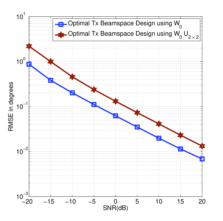
Figure 1: Example 1: Performance of the new proposed method with and without uniform power distribution across transmit waveforms.

V-B Example 2 : Two Separated Sectors of Width $20^{\circ}$ Degrees Each

In the second example, two targets are assumed to lie within two spatial sectors: one from $\theta=[-40^{\circ}\ -20^{\circ}]$ and the other from $\theta=[30^{\circ}\ 50^{\circ}]$. The targets are located at $\theta_{1}=-33^{\circ}$ and $\theta_{2}=41^{\circ}$. Fig. 2 shows the transmit beampatterns of the traditional MIMO with uniform transmit power distribution and both the optimal and SDD designs for ${\bf W}$. It can be seen in the figure that the optimal transmit beamspace method provides the most even concentration of power in the desired sectors. The SDD technique provides concentration of power in the desired sectors above and beyond traditional MIMO; however, the energy is not evenly distributed with one sector having a peak beampattern strength of 15 dB, while the other has a peak of no more than 12 dB. Fig. 3 shows the individual beampatterns associated with individual waveforms as well as the coherent addition of all four individual beampatterns.

The performance of all three methods is compared in terms of the corresponding RMSEs versus SNR as shown in Fig. 4. As we can see in the figure, the jointly optimal transmit beamspace and the SDD methods have lower RMSEs as compared to the RMSE of the traditional MIMO radar. It is also observed from the figure that the performance of the SDD method is very close to the performance of the jointly optimal one.

To assess the proposed method’s ability to resolve closely located targets, we move both targets to the locations $\theta_{1}=38^{\circ}$ and $\theta_{2}=40^{\circ}$. The performance of all three methods tested is given in terms of the probability of target resolution. Note that the targets are considered to be resolved if there are at least two peaks in the MUSIC spectrum and the following is satisfied [2]

$$\left|\hat{\theta}_{l}-\theta_{l}\right|\leq\frac{\Delta\theta}{2},\quad l=1,2$$

where $\Delta\theta=|\theta_{2}-\theta_{1}|$. The probability of source resolution versus SNR for all methods tested are shown in Fig. 5. It can be seen from the figure that the SNR threshold at which the probability of target resolution transitions from very low values (i.e., resolution fail) to values close to one (i.e., resolution success) is lowest for the jointly optimal transmit beamspace design-based method, second lowest for the SDD method, and finally, highest for the traditional MIMO radar method. In other words, the figure shows that the jointly optimal transmit beamspace design-based method has a higher probability of target resolution at lower values of SNR than the SDD method, while the traditional MIMO radar method has the worst resolution performance.

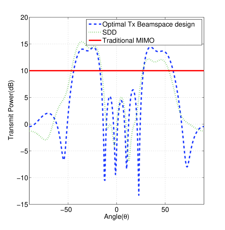
Figure 2: Example 2: Transmit beampatterns of the traditional MIMO and the proposed transmit beamspace design-based methods.

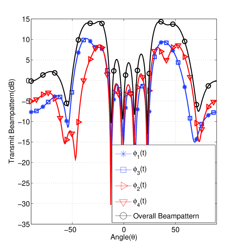
Figure 3: Example 2: Individual beampatterns associated with individual waveforms and the overall beampattern.

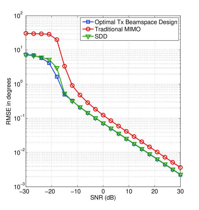
Figure 4: Example 2: Performance comparison between the traditional MIMO and the proposed transmit beamspace design-based methods.

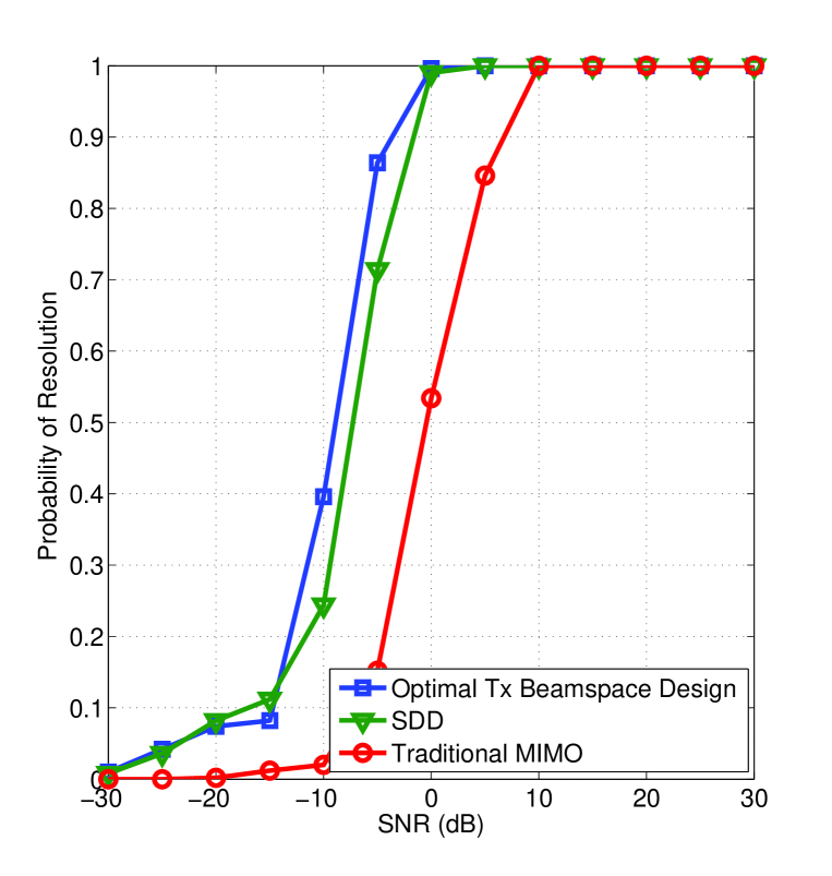
Figure 5: Example 2: Performance comparison between the traditional MIMO and the proposed transmit beamspace design-based methods.

V-C Example 3 : Single and Centrally Located Sector of Width $10^{\circ}$ Degrees

In the third example, the targets are assumed to lie within a single thin sector of $\theta=[-10^{\circ}\ 0^{\circ}]$. Due to the choice of the width of the sector, the optimal number of waveforms to use is only two. For this reason, only two methods are tested: the proposed transmit beamspace method and the traditional MIMO radar. The beampatterns for these two methods are shown in Fig. 6. It can observed from the figure that our method offers a transmit power gain that is 5 dB higher than the traditional MIMO radar. In order to test the RMSE performance of both methods, targets are assumed to be located at $\theta_{1}=-7^{\circ}$ and $\theta_{2}=-2^{\circ}$. The RMSE’s are plotted versus SNR in Fig. 7. It can be observed from this figure that the proposed transmit beamspace method yields lower RMSE as compared to the traditional MIMO radar based method at moderate and high SNR values. At low SNR values one can observe from the figure that the RMSE of the transmit beamspace method saturates at $3^{\circ}$ due to the fact that each of the two targets is located $3^{\circ}$ from the edge of the sector. In order to test the resolution capabilities of both methods tested, the targets are moved to $\theta_{1}=-3^{\circ}$ and $\theta_{2}=-1^{\circ}$. The same criterion as in Example 2 is then used to determine the target resolution. The results of this test are displayed in Fig. 8 and agrees with the similar results in Example 2.

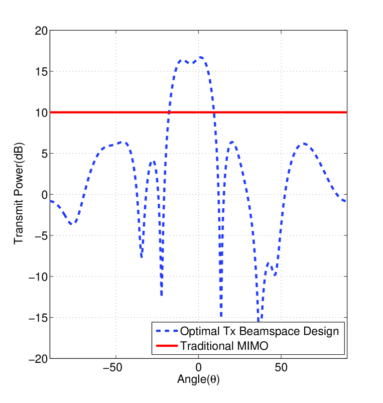
Figure 6: Example 3: Transmit beampatterns of the traditional MIMO and the proposed transmit beamspace design-based method.

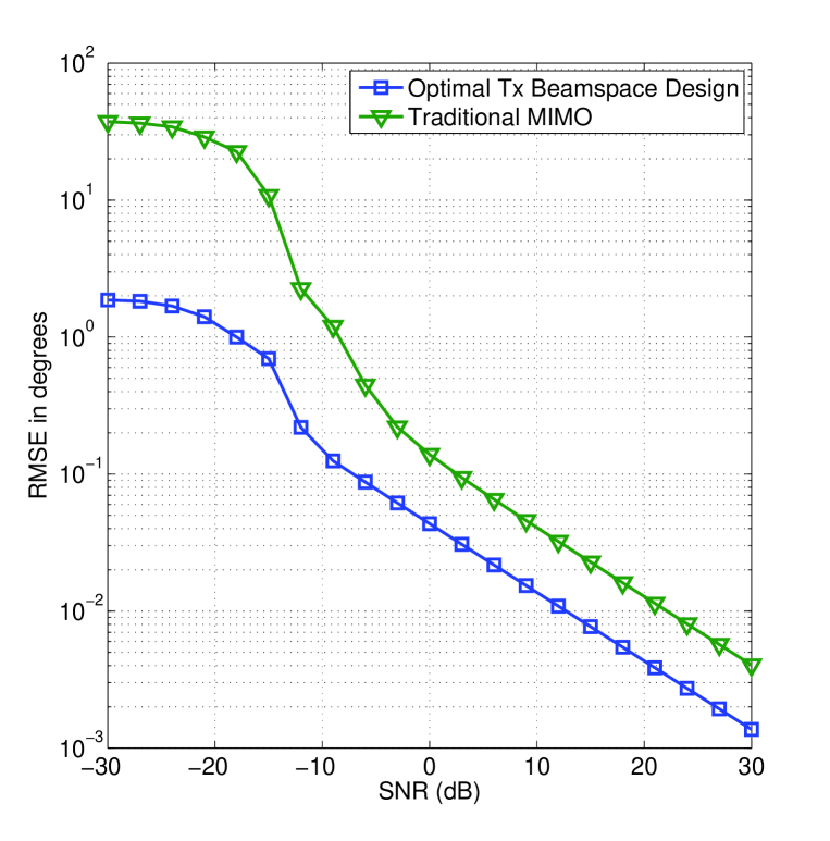
Figure 7: Example 3: Performance comparison between the traditional MIMO and the proposed transmit beamspace design-based method.

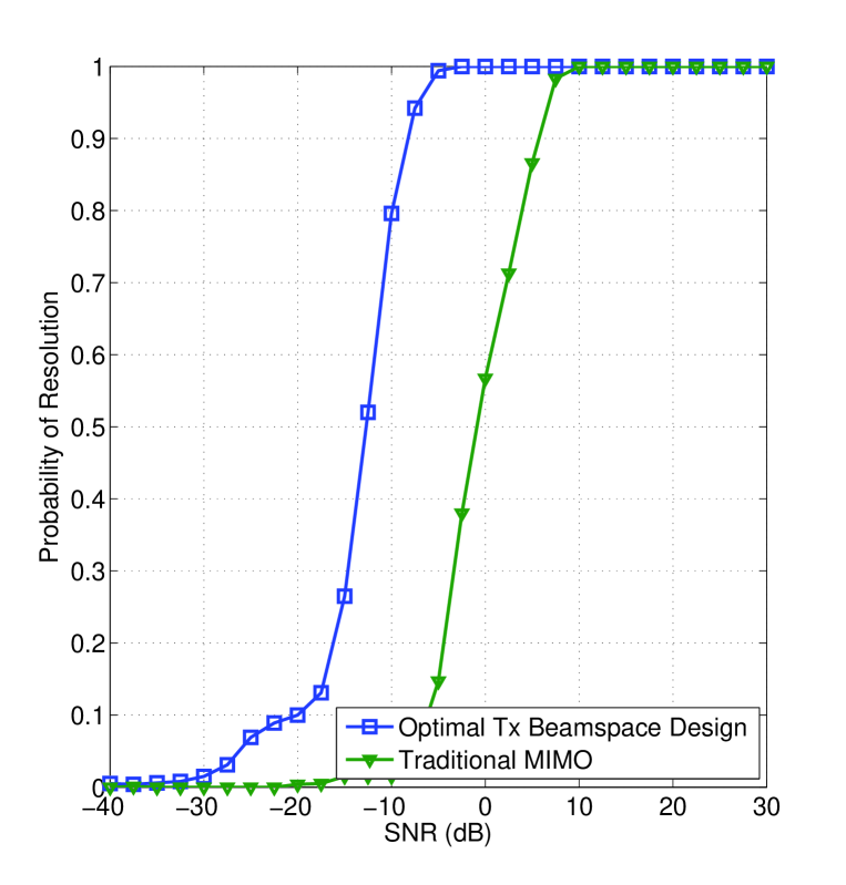
Figure 8: Example 3: Performance comparison between the traditional MIMO and the proposed transmit beamspace design-based methods.

V-D Example 4 : Single and Centrally Located Sector of Width $30^{\circ}$ Degrees

In the last example, a single wide sector is chosen as $\theta=[-15^{\circ}\ 15^{\circ}]$. The optimal number of waveforms for such a sector is found to be four. Similar to the previous Example 3, we compare the performance of the proposed method to that of the traditional MIMO radar. Four transmit beams are used to simulate the optimal transmit beamspace design-based method. Fig. 9 shows the transmit beampatterns for the methods tested. In order to test the RMSE performance of the methods tested, two targets are assumed to be located at $\theta_{1}=-12^{\circ}$ and $\theta_{2}=9^{\circ}$. Fig. 10 shows the RMSEs versus SNR for the methods tested. As we can see in the figure, the RMSE for the jointly optimal transmit beamspace design-based method is lower than the RMSE for the traditional MIMO radar based method. Moreover, in order to test resolution, the targets are moved to $\theta_{1}=-3^{\circ}$ and $\theta_{2}=-1^{\circ}$. The same criterion as in Example 2 is used to determine the target resolution. The results of this test are similar to those displayed in Fig. 5, and, therefore, are not displayed here.

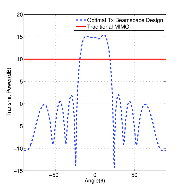
Figure 9: Example 4: Transmit beampatterns of the traditional MIMO and the proposed methods.

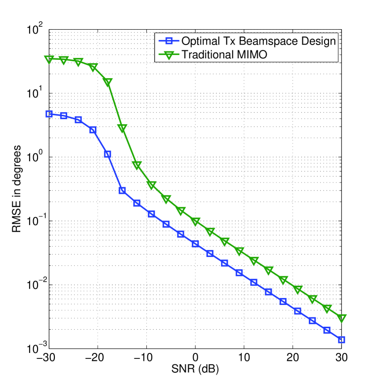
Figure 10: Example 4: Performance comparison between the traditional MIMO and the proposed methods.

VI Conclusion

The problem of transmit beamspace design for MIMO radar with colocated antennas with application to DOA estimation has been considered. A new method for designing the transmit beamspace matrix that enables the use of search-free DOA estimation techniques at the receiver has been introduced. The essence of the proposed method is to design the transmit beamspace matrix based on minimizing the difference between a desired transmit beampattern and the actual one. The case of even but otherwise arbitrary number of transmit waveforms has been considered. The transmit beams are designed in pairs where all pairs are designed jointly while satisfying the requirements that the two transmit beams associated with each pair enjoy rotational invariance with respect to each other. Unlike previous methods that achieve phase rotation between two transmit beams while allowing the magnitude to be different, a specific beamspace matrix structure achieves phase rotation while ensuring that the magnitude response of the two transmit beams is exactly the same at all spatial directions has been proposed. The SDP relaxation technique has been used to transform the proposed formulation into a convex optimization problem that can be solved efficiently using interior point methods. An alternative SDD method that divides the spatial domain into several subsectors and assigns a subset of the transmit beamspace pairs to each subsector has been also developed. The SDD method enables post processing of data associated with different subsectors independently with DOA estimation performance comparable to the performance of the joint transmit beamspace design-based method. Simulation results have been used to demonstrate the improvement in the DOA estimation performance offered by using the proposed joint and SDD transmit beamspace design methods as compared to the traditional MIMO radar.

References

- [1] H. Krim and M. Viberg, “Two decades of array signal processing research: the parametric approach,” IEEE Signal Processing Mag., vol. 13, no. 4, pp. 67–94, Aug. 1996.
- [2] H. Van Trees, Optimum Array Processing. Willey, 2002.
- [3] E. Fishler, A. Haimovich, R. Blum, D. Chizhik, L. Cimini, and R. Valenzuela, “MIMO radar: An idea whose time has come,” in Proc. IEEE Radar Conf., Honolulu, Hawaii, USA, Apr. 2004, vol. 2, pp. 71–78.
- [4] J. Li and P. Stoica, MIMO Radar Signal Processing. New Jersy: Wiley, 2009.
- [5] A. Haimovich, R. Blum, and L. Cimini, “MIMO radar with widely separated antennas,” IEEE Signal Processing Mag., vol. 25, pp. 116–129, Jan. 2008.
- [6] A. De Maio, M. Lops, and L. Venturino, “Diversity-integration tradeoffs in MIMO detection,” IEEE Trans. Signal Processing, vol. 56, no. 10, pp. 5051–5061, Oct. 2008.
- [7] A. Hassanien, S. A. Vorobyov, and A. B. Gershman, “Moving target parameters estimation in non-coherent MIMO radar systems,” IEEE Trans. Signal Processing, vol. 60, no. 5, pp. 2354–2361, May 2012.
- [8] M. Akcakaya and A. Nehorai, “MIMO radar sensitivity analysis for target detection,”IEEE Trans. Signal Processing, vol. 59, no. 7, pp. 3241–3250, Jul. 2011.
- [9] J. Li and P. Stoica, “MIMO radar with colocated antennas,” IEEE Signal Processing Mag., vol. 24, pp. 106–114, Sept. 2007.
- [10] A. Hassanien and S. A. Vorobyov, “Transmit/receive beamforming for MIMO radar with colocated antennas,” in Proc. IEEE Inter. Conf. Acoustics, Speech, and Signal Processing, Taipei, Taiwan, Apr. 2009, pp. 2089-2092.
- [11] P. P. Vaidyanathan and P. Pal, “MIMO radar, SIMO radar, and IFIR radar: A comparison,” in Proc. 63rd Asilomar Conf. Signals, Syst. and Comput., Pacific Grove, CA, Nov. 2009, pp. 160–167.
- [12] A. Hassanien and S. A. Vorobyov, “Phased-MIMO radar: A tradeoff between phased-array and MIMO radars,” IEEE Trans. Signal Processing, vol. 58, no. 6, pp. 3137–3151, Jun. 2010.
- [13] A. Hassanien and S. A. Vorobyov, “Why the phased-MIMO radar outperforms the phased-array and MIMO radars,” in Proc. 18th European Signal Processing Conf., Aalborg, Denmark, Aug. 2010, pp. 1234–1238.
- [14] D. Wilcox and M. Sellathurai, “On MIMO radar subarrayed transmit beamforming,” IEEE Trans. Signal Processing, vol. 60, no. 4, pp. 2076–2081, Apr. 2012.
- [15] A. Hassanien and S. A. Vorobyov,, “Transmit energy focusing for DOA estimation in MIMO radar with colocated antennas,” IEEE Trans. Signal Processing, vol. 59, no. 6, pp. 2669–2682, Jun. 2011.
- [16] G. Hua and S. S. Abeysekera, “Receiver design for range and doppler sidelobe suppression using MIMO and phased-array radar,” IEEE Trans. Signal Processing, vol. 61, no. 6, pp. 1315–1326, Mar. 2013.
- [17] C. Duofang, C. Baixiao, and Q. Guodong, “Angle estimation using ESPRIT in MIMO radar,” Electron. Lett., vol. 44, no. 12, pp. 770–771, Jun. 2008.
- [18] D. Nion and N. D. Sidiropoulos, “Tensor algebra and multidimensional harmonic retrieval in signal processing for MIMO radar,” IEEE Trans. Signal Processing, vol. 58, no. 11, pp. 5693–5705, Nov. 2010.
- [19] D. Fuhrmann, J. Browning, M. Rangaswamy, “Signaling strategies for the hybrid MIMO phased-array radar,” IEEE J. Sel. Topics Signal Processing, vol. 4, no. 1, pp. 66- 78, Feb. 2010.
- [20] D. Fuhrmann and G. San Antonio, “Transmit beamforming for MIMO radar systems using signal cross-correlation,” IEEE Trans. Aerospace and Electronic Systems, vol. 44, no. 1, pp. 171–186, Jan. 2008.
- [21] T. Aittomaki and V. Koivunen, “Beampattern optimization by minimization of quartic polynomial,” in Proc. 15 IEEE/SP Statist. Signal Process. Workshop, Cardiff, U.K., Sep. 2009, pp. 437 440.
- [22] H. He, P. Stoica, and J. Li, “Designing unimodular sequence sets with good correlations–Including an application to MIMO radar,” IEEE Trans. Signal Processing, vol. 57, no. 11, pp.4391–4405, Nov. 2009.
- [23] A. Hassanien and S. A. Vorobyov, “Direction finding for MIMO radar with colocated antennas using transmit beamspace preprocessing,” in Proc. IEEE Int. Workshop on Computational Advances in Multi-Sensor Adaptive Processing (CAMSAP’09), Aruba, Dutch Antilles, Dec. 2009, pp. 181–184.
- [24] V. Tarokh, H. Jafarkhani, and A. R. Calderbank, “Space-time block codes from orthogonal designs,” IEEE Trans. Inf. Theory, vol. 45, no. 7, pp. 1456 1467, Jul. 1999.
- [25] A. Khabbazibasmenj, S. A. Vorobyov, and A. Hassanien, “Transmit beamspace design for direction finding in colocated MIMO radar with arbitrary receive array,” in Proc. 36th IEEE Inter. Conf. Acoustics, Speech, and Signal Processing, Prague, Czech Republic, May 2011, pp. 2784-2787.
- [26] A. Khabbazibasmenj, S. A. Vorobyov, A. Hassanien, M.W. Morency, “Transmit beamspace design for direction finding in colocated MIMO radar with arbitrary receive array and even number of waveforms,” in Proc. 46th Asilomar Conf. Signals, Syst, and Comput., Pacific Grove, CA, Nov. 4-7, 2012.
- [27] Z.-Q. Luo, W.-K. Ma, A. M.-C. So, Y. Ye, and S. Zhang, “Semidefinite Relaxation of Quadratic Optimization Problems,” IEEE Signal Processing Mag., vol. 27, no. 3, pp. 20-34, May 2010.
- [28] A. d’Aspremont and S. Boyd, “Relaxation and randomized method for nonconvex QCQPs,” class note, http://www.stanford.edu/class/ee392o/.
- [29] H. Wolkowicz, “Relaxations of Q2P,” in Handbook of Semidefinite Programming: Theory, Algorithms, and Applications, H. Wolkowicz, R. Saigal, and L.Venberghe, Eds. Norwell, MA: Kluwer, 2000, ch. 13.4.
- [30] A. Khabbazibasmenj, S. A. Vorobyov, and A. Hassanien, “Robust adaptive beamforming based on steering vector estimation with as little as possible prior information,” IEEE Trans. Signal Processing, vol. 60, no. 6, pp. 2974–2987, Jun. 2012.
- [31] K. T. Phan, S. A. Vorobyov, N. D. Sidiropoulos, and C. Tellambura, “Spectrum sharing in wireless networks via QoS-aware secondary multicast beamforming,” IEEE Trans. Signal Processing, vol. 57, no. 6, pp. 2323-2335, Jun. 2009.
- [32] T. E. Abrudan, J. Eriksson, and V. Koivunen, “Steepest descent algorithms for optimization under unitary matrix constraint,” IEEE Trans. Signal Process., vol. 56, no. 3, pp. 1134- 1147, Mar. 2008.
- [33] P. -A. Absil, R. Mahony, and R. Sepulchre, “Riemannian geometry of Grassmann manifolds with a view on algorithmic computation,” Acta Applicandae Mathematicae, vol. 80, no. 2, pp. 199 -220, 2004.