Estimating network degree distributions under sampling: An inverse problem, with applications to monitoring social media networks

Abstract

Networks are a popular tool for representing elements in a system and their interconnectedness. Many observed networks can be viewed as only samples of some true underlying network. Such is frequently the case, for example, in the monitoring and study of massive, online social networks. We study the problem of how to estimate the degree distribution—an object of fundamental interest—of a true underlying network from its sampled network. In particular, we show that this problem can be formulated as an inverse problem. Playing a key role in this formulation is a matrix relating the expectation of our sampled degree distribution to the true underlying degree distribution. Under many network sampling designs, this matrix can be defined entirely in terms of the design and is found to be ill-conditioned. As a result, our inverse problem frequently is ill-posed. Accordingly, we offer a constrained, penalized weighted least-squares approach to solving this problem. A Monte Carlo variant of Stein’s unbiased risk estimation (SURE) is used to select the penalization parameter. We explore the behavior of our resulting estimator of network degree distribution in simulation, using a variety of combinations of network models and sampling regimes. In addition, we demonstrate the ability of our method to accurately reconstruct the degree distributions of various sub-communities within online social networks corresponding to Friendster, Orkut and LiveJournal. Overall, our results show that the true degree distributions from both homogeneous and inhomogeneous networks can be recovered with substantially greater accuracy than reflected in the empirical degree distribution resulting from the original sampling.

FLA

, and T1Supported in part by AFOSR award 12RSL042 and NSF Grant CNS-0905565.

1 Introduction

Many networks observed or investigated today are samples of much larger networks [Kolaczyk (2009), Chapter 5]. Let $G=(V,E)$ be a graph representing a network, with vertex set $V$ and edge set $E$. Similarly, let $G^{*}=(V^{*},E^{*})$ denote a subgraph of $G$, representing a part of the network obtained through some sort of network sampling. Although practitioners typically speak of the network when presenting empirical results, frequently it is only a sampled version $G^{*}$ (or some function thereof, such as when sampling yields estimates of vertex degrees directly) of some true underlying network $G$ that is available to them, either by default or design. A central statistical question in such studies, therefore, is how much the properties of the sampled network reflect those of the true network.

Sampling is of particular interest in the context of online social networks. One reason for such interest is that these networks are usually very large. For example, social networks from Friendster, LiveJournal, Orkut and Amazon have been studied in Yang and Leskovec (2012) having, respectively, $117.7M,4.0M,3.0M$ and $0.33M$ vertices and $2586.1M$, $34.9M$, $117.2M$ and $0.92M$ edges. Similarly in Ribeiro and Towsley (2010), networks from Flickr and Youtube were studied having millions of vertices and edges as well. The large size of these social networks makes it costly querying the entire network, particularly if the goal is to monitor these networks regularly over time. In addition, the decentralized nature of many such networks frequently means that few—if any—people or organizations have complete access to the data.

The topic of network sampling goes back at least to the seminal work of Ove Frank and his colleagues, starting in the late 1960s and extending into the mid-1980s. See Frank (2005), for example, for a relatively recent survey of that literature. With the modern explosion of interest in complex networks, there was a resurgence of interest in sampling. Initially, the focus was on the simple awareness, and then understanding of whether and how sampling affects the extent to which the shape of the degree distribution of the observed network $G^{*}$ reflects that of the true network $G$. Seminal work during this period includes an important empirical study by Lakhina et al. (2003), in the context of traceroute sampling in the Internet, with follow-up theoretical work by Achlioptas et al. (2005), and work by Stumpf and colleagues [e.g., Stumpf and Wiuf (2005), Stumpf, Wiuf and May (2005)], motivated, among other things, by networks arising in computational biology.

The focus on sampling of online social networks, as described above, is arguably the most recent direction in this literature, with a flurry of papers appearing in just the past five years. One of the first papers to look closely at the implications of sampling in very large social media networks (among others) was by Leskovec and Faloutsos (2006), where attention was primarily on more classical network sampling designs (e.g., so-called induced and incident subgraph sampling). This was followed by papers like those by Hubler et al. (2008) and Ribeiro and Towsley (2010), wherein samplers based on principles of the Monte Carlo Markov chain were introduced and explored. Other examples in this highly active area include Ahn et al. (2007), Ahmed et al. (2010), Ahmed, Neville and Kompella (2011), Ahmed, Neville and Kompella (2012), Maiya and Berger-Wolf (2010a), Maiya and Berger-Wolf (2010b), Li and Yeh (2011), Yoon et al. (2011), Shi et al. (2008), Mislove et al. (2007), Lu and Bressan (2012), Lim et al. (2011), Gjoka et al. (2010), Gjoka et al. (2011), Wang et al. (2011), Zhou et al. (2011), Kurant et al. (2011), Kurant, Markopoulou and Thiran (2011), Salehi et al. (2011), Mohaisen et al. (2012), and Jin et al. (2011).

In all of these papers, there is a keen interest in understanding the extent to which characteristics of the network $G^{*}$ are reflective of those of $G$. Typical characteristics of interest include degree distribution, density, diameter, the distribution of the clustering coefficient, the distribution of sizes of weakly (strongly) connected components, Hop-plot, distribution of singular values (vectors) of the network adjacency matrix, the graphlet distribution, the vertex (edge) label density and the assortative mixing coefficient.

Here, in this paper, the network property we focus on is degree distribution. The degree distribution of a network $G$, denoted by $\{f_{d}\}$, specifies the proportion $f_{d}$ of vertices to have exactly $d$ incident edges, for $d=0,1,\ldots.$ It is arguably the most fundamental quantity associated with a network and, importantly, one that may be adversely affected by sampling, sometimes dramatically so [e.g., Lakhina et al. (2003), Stumpf, Wiuf and May (2005)], hence, the following basic question: how do we recover the degree distribution of some true underlying network $G$, given only the information provided by the sampled network $G^{*}$? For simplicity of exposition, hereafter we use the term true degree distribution and observed degree distribution to represent the degree distribution of $G$ and $G^{*}$, respectively.

Frank (1980, 1981) shows that, under certain network sampling designs, the expectation of the observed degree relative frequencies is a linear combination of the true degree relative frequencies. Let $\mathbf{f}=(f_{k})$ and $\mathbf{f}^{*}=(f_{k}^{*})$ be the vectors of true and observed degree frequencies in $G$ and $G^{*}$, respectively. Then

$$E\bigl{[}\mathbf{f}^{*}\bigr{]}=\tilde{P}\mathbf{f},$$ (1)

where $\tilde{P}$ depends fully on the sampling scheme and not on the network itself. Thus, a natural unbiased estimator of $\mathbf{f}$ would seem to be simply $\tilde{P}^{-1}\mathbf{f}^{*}$. However, this estimator suffers from two issues—$\tilde{P}$ typically is not invertible in practice and, even when it is, $\tilde{P}^{-1}\mathbf{f}^{*}$ may not be nonnegative.

From the perspective of nonparametric function and density estimation, what we face is a linear inverse problem. One which, as we show, may potentially be quite ill-posed, in the sense that the matrix $\tilde{P}$ can be quite ill-conditioned. As a result, the estimation of $\mathbf{f}$ must be handled with care, since naive inversion of ill-conditioned operators in inverse problems typically will inflate the “noise” accompanying the process of obtaining measurements, often with devastating effects on our ability to recover the underlying object (e.g., function or density). Here we offer, to the best of our knowledge, the first principled estimator of a true degree distribution $\mathbf{f}$ from a sampled degree distribution $\mathbf{f}^{*}$. In particular, we propose a constrained, penalized weighted least squares estimator, which, in particular, produces estimates that are nonnegative (by constraint) and invert the matrix $\tilde{P}$ in a stable fashion (by construction), in a manner that encourages smooth solutions (through a penalty).

The rest of the paper is organized as follows. In Section 2 we provide a detailed characterization of our inverse problem, discussing the nature of the operator and the distribution of noise. In Section 3 we describe our proposed approach to solving this inverse problem, including a method for the automatic selection of the penalization parameter. In Section 4 we provide results of a simulation study, in which we study the impact on the performance of our estimator of various parameters, including the total number of vertices, the density of the network, sampling rates and network types. In Section 5 we return to the primary application of interest here, that of monitoring online social networks. There we demonstrate the ability of our method to simultaneously reconstruct accurately the degree distributions of various sub-communities within online social networks corresponding to Friendster, Orkut and LiveJournal. Finally, some additional discussion and conclusions may be found in Section 6.

2 Characterizing the inverse problem

In solving inverse problems generally, it is important to understand the nature of both the operator and the noise. Here the operator, in the form of the matrix $\tilde{P}$, will derive entirely from the network sampling design. At the same time, the “noise” (or, more formally, the randomness in our measurements) also derives from the sampling design. This linking of both operator and noise to our sampling lends a certain element of uniqueness to our particular inverse problem, the nature of which we aim to characterize in this section.

2.1 Nature of the problem

To begin with, assume we know the total number of vertices $n_{v}$ in the underlying network. This is a reasonable assumption in the cases of, for example, sampling a phone call network or surveying among a class of students for their interactions. It is also not unreasonable in the context of many online social networks where, for example, this may either be readily available to those who own the network or reported to the community as a basic summary statistic (e.g., the number of members with active pages on Facebook). Thus, we know the degree distribution $\mathbf{f}$ if and only if we know the degree counts $\mathbf{N}=(N_{0},N_{1},\ldots,N_{M})$, where $N_{k}$ is the number of vertices of degree $k$, and $M$ is the maximum degree in the true network $G$. In principle, the largest possible value for $M$ is $n_{v}-1$ in a simple network where no multiple edges or self-loops exist, although in practice we may have knowledge that it is smaller.

Under a given network sampling design, let $P(i,j)$ be the probability that a vertex of degree $j$ in $G$ is selected and observed to have degree $i$ in $G^{*}$. Following Frank (1980, 1981), we will assume that the matrix $P=[P(i,j)]$ of such probabilities depends only on the sampling design and not, in particular, on the network $G$ itself. Then the equation

$$E\bigl{[}\mathbf{N}^{*}\bigr{]}=P\mathbf{N}$$ (2)

holds, in analogy to (1), where $\mathbf{N}^{*}=(N_{0}^{*},N_{1}^{*},\ldots,N_{M}^{*})$ is the vector of observed degree counts in $G^{*}$ and $P=\frac{n_{v}^{*}}{n_{v}}\tilde{P}$ replaces $\tilde{P}$. Without loss of generality, we will restrict our attention to this formulation of our problem for the remainder of the paper.

It is useful to proceed with our characterization within the context of the naive estimator of $\mathbf{N}$ obtained simply by inverting $P$, that is,

$$\hat{\mathbf{N}}_{\mathrm{naive}}=P^{-1}\mathbf{N}^{*},$$ (3)

where, again, we note that a formal inverse may or may not be well-defined. The singular value decomposition (SVD) is a canonical tool for studying the behavior of this estimator. Let $P=UDV^{T}$, where $D=\operatorname{diag}(d_{0},d_{1},\ldots,d_{M})$ is a diagonal matrix of singular values, and $U=(\mathbf{u}_{0},\mathbf{u}_{1},\ldots,\mathbf{u}_{M})$, $V=(\mathbf{v}_{0},\mathbf{v}_{1},\break\ldots,\mathbf{v}_{M})$ are orthogonal matrices of the left- and right-singular vectors, respectively. Then

$$\hat{\mathbf{N}}_{\mathrm{naive}}=\sum_{i=0}^{M}\biggl{[}\frac{1}{d_{i}}\mathbf{u}_{i}^{T}\mathbf{N}^{*}\biggr{]}\mathbf{v}_{i}$$ (4)

decomposes the naive estimator (3) into a linear combination of the right singular vectors of $P$.

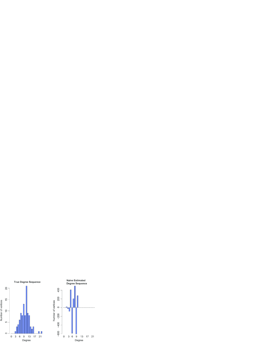
Figure 1: Left: ER graph with 100 vertices and 500 edges. Right: Naive estimate of degree distribution, according to equation (3). Data drawn according to induced subgraph sampling with sampling rate $p=60\%$.

The quality of this estimator is determined, in part, by the extent to which the vector $\mathbf{N}$ may be approximated well by such linear combinations. In general, the right singular vectors $v_{i}$ vary in smoothness, from smoother behavior (i.e., low-frequency) at small values of $i$ to less smooth behavior (i.e., high-frequency) at larger values of $i$. Since most degree distributions encountered in practice, as well those induced through common choices of random graph models (some examples of which we use in Section 4), are relatively smooth, typically with either exponential or power-law behavior in the tails, intuitively it is the first handful of right singular vectors upon which a sensible estimator should be based. The stability of this estimator can be summarized through the condition number of $P$, that is, the ratio of the largest to smallest singular values. Larger condition numbers suggest greater instability in the estimator. Intuitively, for unstable matrices $P$, the singular values $d_{i}$ at higher indices $i$ are, comparatively, quite small. As a result, the estimator in (4) will put disproportionately large weight on contributions from the latter (i.e., high-frequency) singular vectors. The end result is an estimator that can oscillate in a decidedly unappealing manner, as illustrated in Figure 1.

Since the operator $P$ plays such an important role in both the shape and the stability of the estimator (and, by extension, more sensible modifications of the estimator, such as we offer below), and $P$ in turns is determined by the sampling design, we examine a handful of canonical examples of sampling designs and their operators in the following subsection.

2.2 Common network sampling designs and the operator $P$

Here we look at a few common network sampling designs and their corresponding $P$ matrix. We consider them ordered from simpler to more complex. We refer readers to Kolaczyk (2009, Chapter 5) for additional background on network sampling and a more comprehensive list of sampling designs.

2.2.1 Ego-centric and one-wave snowball sampling

Ego-centric sampling (also called unlabeled star sampling) is a simple, nonadaptive (conventional) sampling design. As Handcock and Gile (2010) write that “[a] sampling design is conventional if it does not use information collected during the survey to direct subsequent sampling of individuals$\ldots$ [and] a sampling design [is] adaptive if it uses information collected during the survey to direct subsequent sampling, but the sampling design depends only on the observed data.” Under ego-centric sampling, first a set of vertices is selected according to independent $\operatorname{Bernoulli}(p)$ trials at each vertex. Then all edges incident to the selected vertices are observed. In this case, the operator $P$ is a diagonal matrix with the sampling rate $p$ at each diagonal position, that is,

$$P_{\mathrm{ego}}(i,j)=\cases{p,&$\quad\mbox{for }i=j=0,1,\ldots,M$,\vspace*{3pt}\cr 0,&\quad$\mbox{for }i,j=0,\ldots,M;i\neq j$.}$$ (5)

A natural extension of this concept is one-wave snowball sampling. Here, after an initial selection of vertices, there is a subsequent selection of additional vertices, using the information obtained from the initial selection. Therefore, one-wave snowball sampling is an adaptive sampling design. The initial selection is again done according to independent $\operatorname{Bernoulli}(p)$ trials. The subsequent selection contains all vertices that have at least one connection with a vertex in the initial set. Similar to ego-centric sampling, all edges incident to vertices selected in either of the two sets are then observed, so the operator $P$ is again a diagonal matrix, with entries

$$P_{\mathrm{snow}}(i,j)=\cases{1-(1-p)^{i+1},&\quad$\mbox{for }i=j=0,1,\ldots,M$,\vspace*{3pt}\cr 0,&\quad$\mbox{for }i,j=0,\ldots,M;i\neq j$.}$$ (6)

These two sampling designs (as well as multi-wave snowball sampling and other variations) are common in social network studies, where, for example, a selection of individuals are interviewed and asked to nominate their connections or partners. Readers can refer to Rolls et al. (2012) for more details, in the context of networks of injecting drug users. We note that the adaptive designs we consider here are the textbook versions and not complicated adaptations that might sometimes be used in practice due to resource limitations for following links. Even so, the standard and simple designs we consider with known and constant matrix $P$ would be the logical point of departure for research on correcting the sampling bias of the degree distribution in more complex adaptive designs.

For a diagonal $P$ matrix, the singular values are equal to the diagonal elements. Both the left and right singular vectors are the canonical set of basis vectors $\{e_{i}\}_{i=1}^{M+1}$, where $e_{i}$ contains a $1$ at the $i$th entry and $0$ at all the other entries. Since $P_{\mathrm{ego}}=I\times p$, where $I$ is the identity matrix, $P_{\mathrm{ego}}$ is not ill-conditioned at all. To estimate the degree count vector $\mathbf{N}$, we need only scale the observed degree count vector $\mathbf{N}^{*}$ by $1/p$. That is, the naive estimator is $\hat{N}_{\mathrm{naive}}=N^{*}/p$.

In one-wave snowball sampling, the observed degree counts are biased, because in the second round of vertex selection, there is more chance to select the vertices that have more connections. The observed degree count vector therefore can be thought of as moving to the right of the true degree count vector. Hence, at a minimum, a good estimator should correct the observations by moving the distribution back to the left. How difficult this task may be is summarized by the condition number of $P_{\mathrm{snow}}$, which is equal to

$$\frac{P_{\mathrm{snow}}(M,M)}{P_{\mathrm{snow}}(0,0)}=\frac{1-(1-p)^{M+1}}{1-(1-p)}=\frac{1-(1-p)^{M+1}}{p},$$ (7)

and therefore depends on the relationship between the expected proportion $p$ of vertices sampled initially and the maximum degree $M$. In the case where $p$ is fixed, as $M$ increases, the condition number is upper bounded by $\frac{1}{p}$. On the other hand, if $Mp=o(1)$, using the approximation $(1-p)^{M+1}\approx 1-(M+1)p$, we find that the condition number behaves as $(M+1)$.

These observations suggest that, for instance, under low sampling rates the inverse problem is increasingly ill-posed for estimating degree distributions of heavier tails. Also, the bounds on the condition numbers suggest that, in contrast to estimation of the mean from a sample from a finite population, where the accuracy depends on the sample size rather than the fraction of the population that is sampled, for estimation of complex properties of networks the accuracy depends strongly on the fraction of the population that is sampled.

2.2.2 Induced and incident subgraph sampling

These two sampling designs are both nonadaptive and analogous in spirit, differing only in the order of selection of vertices and edges. In induced subgraph sampling, a set of vertices is selected as independent $\operatorname{Bernoulli}(p)$ trials (other variations are possible—see below). Then, all edges between selected vertices are observed, that is, we observe the subgraph induced by this vertex subset. This sampling scheme has been used in the analysis of technological and biological networks [Stumpf and Wiuf (2005)]. Conversely, under incident subgraph sampling we select edges as independent $\operatorname{Bernoulli}(p)$ trials and we then observe all vertices incident to at least one selected edge.

The $P$ matrix for induced subgraph sampling is

$$P_{\mathrm{ind}}(i,j)=\cases{\displaystyle\pmatrix{j\cr i}p^{i+1}(1-p)^{j-i},&\quad$\mbox{for }0\leq i\leq j\leq M$,\vspace*{3pt}\cr 0,&\quad$\mbox{for }0\leq j<i\leq M$,}$$ (8)

while that for incident subgraph sampling is

$$P_{\mathrm{inc}}(i,j)=\cases{\displaystyle\pmatrix{j\cr i}p^{i}(1-p)^{j-i},&\quad$\mbox{for }1\leq i\leq j\leq M$,\vspace*{3pt}\cr 0,&\quad$\mbox{for }0\leq j<i\leq M$.}$$ (9)

Notice that for incident subgraph sampling the index $i$ starts from $1$, because there are no isolated vertices in the sample.

These two sampling designs are widely studied in literature, for example, in Stumpf and Wiuf (2005), Leskovec and Faloutsos (2006), Ahmed, Neville and Kompella (2011), and Kurant et al. (2012), to name a few. In some cases, simple random sampling (SRS) is used instead of Bernoulli sampling to select the initial vertices or edges. However, under appropriate calibration of $p$, the former can be well approximated by the latter for large networks and small to moderate $p$. So, without loss of generality, we ignore this variant for the purposes of exposition.

Unlike ego-centric and one-wave snowball sampling, the structure of the operator under induced/incident subgraph sampling can cause severe problems if we try to invert it naively. Because the structure of $P_{\mathrm{inc}}$ is very similar to $P_{\mathrm{ind}}$, we only analyze $P_{\mathrm{ind}}$ here. The condition number in this case is equal to $p^{-M}$ and so, as the sampling rate $p$ goes down or the maximum degree $M$ increases, the operator $P$ becomes more ill-conditioned. In real-world situations, such as the monitoring of online social networks, sampling rates are typically low (e.g., 10–20%) and $M$ is typically large (e.g., on the order of 100’s or 1000’s), and thus $P$ is decidedly ill-conditioned and effectively not invertible. The overall pattern of decay of the singular values under induced subgraph sampling is illustrated in Figure 2.

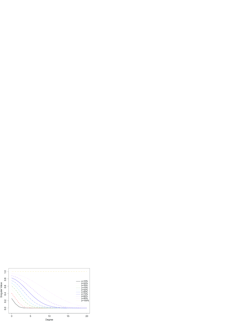
Figure 2: Singular values decay under induced subgraph sampling. $M=20$.

Recall that the decomposition in (4) shows the naive estimator to be a linear combination of the right singular vectors $v_{i}$, with weights determined in part by the inner product of the observations $\mathbf{N}^{*}$ with the left singular vectors $u_{i}$. Examination of these vectors can provide additional insight into the expected behavior of this estimator. As can be seen from the illustration in Figure 3, the right singular vectors behave like a Fourier basis, in that they are supported over the full range of degrees $k$ and oscillate increasingly with higher indices $i$. On the other hand, the left singular vectors, shown in Figure 4, behave in a more stable fashion with increasing index $i$, with only the support changing noticeably at the higher indices, moving like a window from low degrees $k$ to high. Combined with our previous observation of the drastic decay in singular values $d_{i}$, this explains the behavior of the estimate in Figure 1.

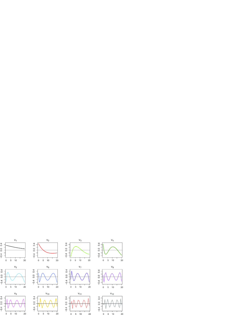
Figure 3: The first 12 right singular vectors under induced subgraph sampling, ordered by singular values from big to small: maximum degree $M=20$, sampling rate $p=20\%$.

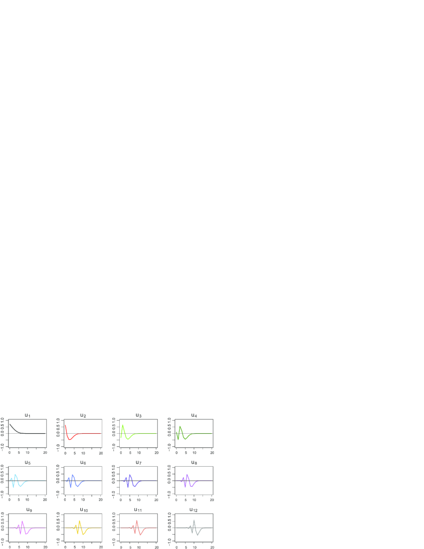
Figure 4: The first 12 left singular vectors under induced subgraph sampling, ordered by singular values from big to small: maximum degree $M=20$, sampling rate $p=20\%$.

While it would be desirable to have an analytical expression for the singular vectors under induced subgraph sampling, we are unable to produce one; however, it is possible to produce expressions for the eigenfunctions of $P_{\mathrm{ind}}$, as solutions to the nonsymmetric eigen-decomposition $P_{\mathrm{ind}}=\tilde{U}\Lambda\tilde{U}^{-1}$. These do not appear to be helpful in yielding similarly interpretable expressions for the SVD but, nonetheless, may be of some independent interest. We therefore include this result in Appendix A.

2.2.3 Random walk and other exploration-based methods

Another class of sampling plans that has arisen recently, and has been of particular interest to the community working with online social networks, is that based on notions of visiting vertices and edges in a network in the course of a random walk on the graph $G$. Specifically, in the basic version of random walk sampling, we first select a vertex $u$ uniformly at random from $V$. Then one of $u$’s neighbor vertices, say $v$, is chosen uniformly at random from the set of $u$’s neighbors. In turn, one of $v$’s neighbor vertices, say $w$, is chosen uniformly at random from the set of $v$’s neighbors. The process is repeated, and the selected vertices $\{u,v,w,\ldots\}$ along with the edges $\{(u,v),(v,w),\ldots\}$ constitute the sample. For examples of other members of this family, we refer readers to Leskovec and Faloutsos (2006) and Ribeiro and Towsley (2010).

If we consider a random walk sampling over a nonbipartite, connected, undirected graph, once the steady state is reached, it shares an important property with incident subgraph sampling with SRS of edges, in that both sample edges uniformly at random [Ribeiro and Towsley (2010)]. Thus,

$$P_{\mathrm{RW}}(i,j)=\cases{\displaystyle\pmatrix{j\cr i}\pmatrix{n_{e}-j\cr n^{*}_{e}-i}\pmatrix{n_{e}\cr n^{*}_{e}}^{-1},&\quad$\mbox{for }1\leq i\leq j\leq M$,\vspace*{3pt}\cr 0,&\quad$\mbox{for }0\leq j<i\leq M$,}$$ (10)

where $n_{e}$ is the total number of edges in the true network and $n^{*}_{e}$ is the number of edges selected in the sample. Therefore, with respect to the nature of the inverse problem that we study here, we may categorize this sampling plan with the induced and incident subgraph sampling plans described above.

2.3 Distribution of the noise

The observation $\mathbf{N}^{*}$ can be viewed as a “noisy” version of $N$. However, as remarked earlier, since it is assumed here that there is no measurement error (e.g., if a query of Facebook indicates person $A$ has “friended” person $B$, then we accept that they have), the “noise” is rather a reflection of the randomness due to sampling. Because we intend to pursue a regression-based approach to solving our linear inverse problem, the question of what noise model to use as an approximation to sampling variability is important. We discuss this question now.

For ego-centric sampling, a vertex is observed to have degree $k$ if and only if the vertex is selected through Bernoulli sampling and also has degree $k$ in the true graph. Therefore,

$$N_{k}^{*}=\sum_{\{u\dvtx d_{u}=k\}}I\bigl{\{}u\in V^{*}\bigr{\}},$$ (11)

where $d_{u}$ represents the degree of a vertex $u\in V$ in $G$, and $d_{u}^{*}$ represents the degree of a vertex $u\in V^{*}$ in $G^{*}$. For each $k$, there are $N_{k}$ such independent indicator functions, and each indicator function has the same probability to be one. Thus, the distribution of the $N_{k}^{*}$ is that of $M+1$ independent binomials, that is, $N_{k}^{*}\sim\operatorname{Bin}(p,N_{k})$. For small $p$ and large $N_{k}$, we can expect that these binomials may be well-approximated as Poisson random variables, with means $N_{k}p$.

The case of one-wave snowball sampling and induced subgraph sampling (as well as the related cases of incident subgraph sampling and random walk sampling) is decidedly less straightforward to analyze. The expectation of $\mathbf{N}^{*}$ is, of course, provided by equation (2). The variance (covariance) formula is more complicated.

For one-wave snowball sampling, the representation (11) still applies. However, the indicator functions are not independent. Straightforward arguments yield that the covariance and variance of $N_{k}^{*}$ for $k=0,1,\ldots,M$ are

$$\operatorname{Cov}\bigl{(}N_{k}^{*},N_{l}^{*}\bigr{)} = \sum_{t}N_{1klt}\bigl{[}1-(1-p)^{l+1}-(1-p)^{k+1}+(1-p)^{k+l-t}\bigr{]}$$

$${}+\sum_{t}N_{0klt}\bigl{[}1-(1-p)^{l+1}-(1-p)^{k+1}+(1-p)^{k+l-t+2}\bigr{]}$$

$${}-N_{k}N_{l}P_{\mathrm{snow}}(k,k)P_{\mathrm{snow}}(l,l)$$

and

$$\operatorname{Var}\bigl{(}N^{*}_{k}\bigr{)} = N_{k}P_{\mathrm{snow}}(k,k)$$

$${}+\sum_{t}N_{1kkt}\bigl{[}1-2(1-p)^{k+1}+(1-p)^{2k-t}\bigr{]}$$

$${}+\sum_{t}N_{0kkt}\bigl{[}1-2(1-p)^{k+1}+(1-p)^{2k-t+2}\bigr{]}$$

$${}-\bigl{(}N_{k}P_{\mathrm{snow}}(k,k)\bigr{)}^{2},$$

where $N_{0klt}$ ($N_{1klt}$) is determined by the underlying network $G$, defined as the number of ordered pairs of nonadjacent (adjacent) distinct vertices of degrees $k$ and $l$, respectively, which have $t$ common adjacent vertices.

For induced-subgraph sampling, we can write

$$N_{k}^{*}=\sum_{r=k}^{M}\sum_{u=1}^{n_{v}}I\bigl{\{}u\in V^{*},d_{u}^{*}=k,d_{u}=r\bigr{\}}.$$ (14)

Using arguments analogous to those in Frank (1980), it is possible to show that, for $k=0,1,\ldots,M$, the variance takes the form

$$\operatorname{Var}\bigl{(}N^{*}_{k}\bigr{)} = \sum_{i}N_{i}P_{\mathrm{ind}}(k,i)$$

$${}+\sum_{r}\sum_{s}\sum_{t}N_{0rst}\sum_{m}\pmatrix{t\cr m}\pmatrix{r-t\cr k-m}\pmatrix{s-t\cr k-m}$$

$$\hskip 100.0pt{}\times p^{2k-m+2}q^{(r+s-t)-(2k-m)}$$

$${}+\sum_{r}\sum_{s}\sum_{t}N_{1rst}\sum_{m}\pmatrix{t\cr m}\pmatrix{r-t-1\cr k-m-1}\pmatrix{s-t-1\cr k-m-1}$$

$$\hskip 100.0pt{}\times p^{2k-m}q^{(r+s-t)-(2k-m)}$$

$${}-(\sum_{i}N_{i}P_{\mathrm{ind}}(k,i))^{2}.$$

Using similar techniques, it is also possible to write out a similar formula for $\operatorname{Cov}(N_{j}^{*},N_{k}^{*})$, which we find is, in general, nonzero for $j\neq k$, as would be expected.

Now consider the marginal distributions of the $N^{*}_{k}$ under snowball sampling and induced subgraph sampling. Note that the first term in (2.3) and (2.3) is the $k$th entry of the expectation $P\mathbf{N}$. This observation suggests that, if the remaining terms in the variance (as well as the off-diagonal terms corresponding to covariances) are sufficiently small, a Poisson model might again be acceptable.

More precisely, if the sampling rate $p$ is small, then each of the indicators in (11) and (14) likely has only very small probability of being equal to one. On the other hand, if the graph is large (i.e., $n_{v}$ is large) and $k$ is not too far out in the tail of the distribution (i.e., $k$ is not too close to $M$), then there should be many such indicators. So a Poisson approximation would make sense here. Given, however, that these indicator variables are dependent, the necessary argument is somewhat more involved. We present a formal justification, using the Chen–Stein method, in Appendix B.

Simulation can be used to assess this approximation. Some representative results, shown in Figure 5, confirm the reasonableness of a Poisson approximation for the marginal distribution of the $N^{*}_{k}$, under induced subgraph sampling, for $k$ within a reasonable distance from the mean.

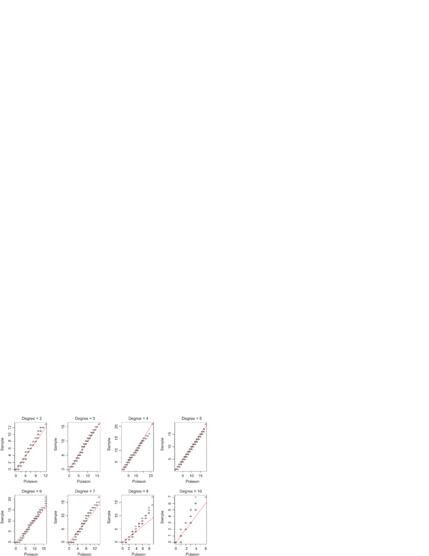
Figure 5: QQ plot: distribution of $N_{i}^{*}$ compared to Poisson distribution with mean $(PN)_{i}$. The underlying network is ER with $n_{v}=|V|=1000$ and $n_{e}=|E|=50{,}000$. Sampling rate $p=5\%$. The average degree of the sample is equal to $5$.

In summary, for all of the sampling plans considered in this paper, an approximate Poisson marginal distribution is arguably reasonable for the observed counts $N^{*}_{k}$. Thus, a Poisson regression model is suggested for solving our inverse problem. However, for reasons of numerical efficiency and stability, we prefer to approximate this model in turn by a Gaussian model, with nonconstant variance that varies in proportion to the mean, leading to a weighted least squares regression. Simulation results (shown in Figure 6) suggest that this, too, is a reasonable choice. Accordingly, our model development, as described starting in the next section, will implicitly assume a Gaussian noise model.

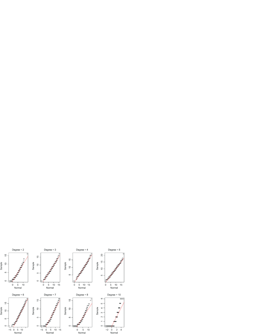
Figure 6: QQ plot: distribution of $N_{i}^{*}$ compared to Gaussian distribution with mean $(PN)_{i}$ and sample variance. The underlying network is ER with $n_{v}=|V|=1000$ and $n_{e}=|E|=50{,}000$. Sampling rate $p=5\%$. The average degree of the sample is equal to $5$.

2.4 Discussion of assumptions

In some sampling designs, nodes’ inclusion probabilities can depend on unobserved properties of the node, such as its true degree, or on other unobserved properties of the network. In this paper we restrict attention to sampling designs (ego-centric, one-wave snowball sampling, induced/incident subgraph sampling, random walk) where inclusion probabilities are known. This restriction underlies (1) and (2) to be established without the need for assumptions about the structure of the network itself. The approach we take is called “design-based” in the sampling literature, as compared to “model-based.” Handcock and Gile (2010) observe the following:

In the design-based framework [$G$] represents the fixed population and interest focuses on characterizing based on partial observation. The random variation considered is due to the sampling design alone. A key advantage of this approach is that it does not require a model for the data themselves$\ldots$ Under the model-based framework, $[G]$ is stochastic and is a realization from a stochastic process depending on a parameter $\eta$. Here interest focuses on $\eta$ which characterizes the mechanism that produced the complete network $[G]$.

Design-based inferences are generally not feasible (i) for adaptive sampling designs other than a network census and ego-centric sampling designs [Handcock and Gile (2010), 11ff] or (ii) for any designs for which the inclusion probabilities of sampled nodes (and dyads, triads, etc., depending on the application) are unknown at least up to a scaling factor. Design-based inference is the standard mode for analysis of samples obtained by government statistical agencies or for large-scale random samples funded by government agencies. That is not to say that assumptions are not brought in for taking into account nonresponse or response error, but the latter two sources of error depend on the properties of the sampled units rather than the sampling design itself. Although design-based inference is applicable only to a restricted set of sample designs, it has the advantage of not requiring specific knowledge about the graph or network being sampled.

We are assuming that the number of nodes is known, consistent with the only other research on design-based inferences for the degree distribution. The assumption is not strictly necessary, as the number of nodes is estimable by a Horvitz–Thompson estimator for the designs under consideration [Handcock and Gile (2010), pages 12–13], but the assumption simplifies the exposition. We also assume that the sampling probabilities of nodes (or edges) are known, which is a standard assumption for conventional sampling designs [e.g., Cochran (1977)] and not unrealistic for the designs we are considering.

We assume as well that the nodes and edges in the sample are observed without error. In the network literature, the question of effect of such observational error and how to quantify and adjust for it is still largely unexplored, and hence is beyond the scope of this paper.

3 Estimating the degree distribution

Bearing in mind the SVD-based representation of the naive estimator $P^{-1}\mathbf{N}^{*}$ of $\mathbf{N}$, as shown in (4), the analyses of Section 2 together suggest that a better solution to our inverse problem would be an estimator developed in a manner analogous to ridge regression and other similar penalized regression strategies. In this section, we offer such an approach.

We adopt a penalized least squares perspective in defining our estimator. Informed by our analysis of the “noise” in our inverse problem, we specify a generalized least squares criterion. Furthermore, since the vector of degree counts should be everywhere nonnegative and, additionally, the total degree counts should equal the total number of vertices, $n_{v}$, we include these two properties as constraints. Our estimator $\hat{\mathbf{N}}$ for $\mathbf{N}$ is then the solution to the following optimization problem:

$$\mathop{\operatorname{minimize}}_{\mathbf{N}}\qquad\bigl{(}P\mathbf{N}-\mathbf{N}^{*}\bigr{)}^{T}C^{-1}\bigl{(}P\mathbf{N}-\mathbf{N}^{*}\bigr{)}+\lambda\cdot\operatorname{pen}(\mathbf{N})$$

$$\mbox{subject to}\qquad N_{i}\geq 0,i=0,1,\ldots M,$$ (16)

$$\phantom{\mbox{subject to}}\qquad\sum_{i=0}^{M}{N_{i}}=n_{v},$$

where $C$ denotes the covariance matrix of $\mathbf{N}^{*}$, that is, $C=\operatorname{Cov}(\mathbf{N}^{*})$, $\operatorname{pen}(\mathbf{N})$ is a penalty on the complexity of $\mathbf{N}$, and $\lambda$ is a smoothing parameter.

Under a convex penalty, (16) has the canonical form of a convex optimization [Boyd and Vandenberghe (2004)] and, in principle, standard software can be used. For example, CVX, a package for specifying and solving convex programs [CVX Research (2012)], can be used to solve (16). In our case, because we use a penalty based on an $\ell_{2}$ norm, as discussed below, (16) can be written as a quadratic programming problem. Accordingly, we use quadprog, the quadratic programming function in the MATLAB optimization toolbox, to solve (16).

Note that the solution spaces of the original problem (2) and (16) are not the same. The solution (3) of the original problem (2) is a point in a space generated by the right singular vectors $\{v_{i}\}$. The constraint and penalized solution of (16) is a point in a space generated by $\{B^{-1}v_{i}\}$, where $B=\bigl{[}{{\matrix{P^{T}C^{-1}P+\lambda\Omega&\tfrac{1}{2}\mathbf{1}\vspace*{-0.5pt}\cr\mathbf{1}^{T}&0}}}\bigr{]}$, ignoring the nonnegativity constraint as is shown in (45). Through this we obtain smoothing.

In the following subsections we discuss choice of the penalty, selection of the smoothing parameter and various practical considerations.

3.1 Penalty

There are a variety of penalties common in the literature on nonparametric function estimation, usually consisting of a norm (e.g., $\ell_{1}$, $\ell_{2}$, total-variation, etc.) applied to some functional of the proposed estimator. The choice of penalty should reflect the assumption of smoothness, that is, $f_{k}\approx f_{l}$ if $k$ and $l$ are close. Examples of networks with smooth degree distributions include Erdös-Rényi (ER), mixture of ER, power-law networks, networks having exponential or power-law tails, as well as those having the body of the exponential or power-law networks. We want to force our estimates toward distributions with such smoothness, where the naive estimates have obvious flaws (e.g., Figure 1).

In our framework, the assumption of a smooth true degree distribution is accounted for by choosing a penalization of the form $\|D\mathbf{N}\|_{2}^{2}$, where the matrix $D$ represents a second-order differencing operator. Specifically, the formula for $D$ is

$$D=\left[\matrix{1&-2&1&0&\cdots&0&0&0&0\vspace*{2pt}\cr 0&1&-2&1&\cdots&0&0&0&0\vspace*{2pt}\cr 0&0&1&-2&\cdots&0&0&0&0\vspace*{2pt}\cr\vdots&\vdots&\vdots&\vdots&&\vdots&\vdots&\vdots&\vdots\vspace*{2pt}\cr 0&0&0&0&\cdots&-2&1&0&0\vspace*{2pt}\cr 0&0&0&0&\cdots&1&-2&1&0\vspace*{2pt}\cr 0&0&0&0&\cdots&0&1&-2&1}\right].$$ (17)

This choice, in the discrete setting, is analogous to the use of a Sobolev norm with nonparametric function estimation in the continuous setting. It assumes mean-square curvature of the degree distribution is small. This is one commonly used smoothing regularization, and we have found it to work well with the types of degree distributions explored here. Other penalties may work less well. For example, the $L1$ norm can be used as a heuristic for finding a sparse solution, thus the solutions $\hat{N}$ can be truncated. We refer readers to Chapter 6.6.6 of Boyd and Vandenberghe (2004) for how different penalty functions perform generally on denoising problems.

3.2 Selection of the penalization parameter $\lambda$

Denote the solution to the optimization problem in (16) as $\hat{\mathbf{N}}=f_{\lambda}(\mathbf{N}^{*})$, a function of $\mathbf{N}^{*}$, indexed by $\lambda$. For a given observation vector $\mathbf{N}^{*}$, a bigger $\lambda$ produces a smoother estimator. The problem of selecting an optimal $\lambda$ falls into the category of model selection. However, commonly used cross-validation methods which assume independent and identically distributed observations do not apply to our network sampling situation because, as already discussed, the $N_{i}^{*}$ for $i=0,\ldots,M$ are not identically distributed and there are nonzero correlations between $N_{i}^{*}$ and $N_{j}^{*}$ for $i\neq j$. Instead, we offer a strategy based on the method of generalized Stein’s unbiased risk estimation (SURE), proposed in Eldar (2009).

We define a weighted mean square error (WMSE) in the observation space as

$$\mathrm{WMSE}(\hat{\mathbf{N}},\mathbf{N})=E\bigl{[}(P\mathbf{N}-P\hat{\mathbf{N}})^{T}C^{-1}(P\mathbf{N}-P\hat{\mathbf{N}})\bigr{]}.$$ (18)

Under the conditions that $f_{\lambda}(\mathbf{N}^{*})$ is weakly differentiable and that $E|f_{\lambda}(\mathbf{N}^{*})|$ is bounded (which we verify following the arguments in Appendix C), a generalized SURE estimate for the WMSE can be obtained as

$$\widehat{\mathrm{WMSE}}(\hat{\mathbf{N}},\mathbf{N}) = (P\mathbf{N})^{T}C^{-1}P\mathbf{N}+(P\hat{\mathbf{N}})^{T}C^{-1}P\hat{\mathbf{N}}$$

$${}+2\biggl{\{}\operatorname{Trace}\biggl{(}P\frac{\partial\hat{\mathbf{N}}}{\partial\mathbf{N}^{*}}\biggr{)}\biggr{\}}$$

$${}-2(P\hat{\mathbf{N}})^{T}C^{-1}\mathbf{N}^{*}.$$

The first term in (3.2) involves the unknown $\mathbf{N}$. However, we may drop this term because it does not involve $\lambda$. The last three terms have $\hat{\mathbf{N}}$ in them, which is a function of $\lambda$. Given $P,\mathbf{N}^{*}$ and $C$ as well, the second and fourth terms are straightforward to compute. The third term, called the divergence term in Eldar (2009), can be simulated using the Monte Carlo technique proposed in Ramani, Blu and Unser (2008). Specifically, let $b$ be a vector with zero mean, covariance matrix $I$ (i.e., independent of $\mathbf{N}^{*})$ and bounded higher order moments. Then

$$\operatorname{div}\equiv\operatorname{Trace}\biggl{(}P\frac{\partial\hat{\mathbf{N}}}{\partial\mathbf{N}^{*}}\biggr{)}=\lim_{\varepsilon\to 0}E_{b}\biggl{\{}b^{T}P\biggl{(}\frac{f_{\lambda}(\mathbf{N}^{*}+\varepsilon\mathbf{b})-f_{\lambda}(\mathbf{N}^{*})}{\varepsilon}\biggr{)}\biggr{\}}.$$ (20)

Let $\mathbf{b_{i}}$ be the realization of $\mathbf{b}$ at each simulation. The algorithm for estimating $\operatorname{div}=\operatorname{Trace}(P\frac{\partial\hat{\mathbf{N}}}{\partial\mathbf{N}^{*}})$ and computing of $\widehat{\mathrm{WMSE}}$ for a given $\lambda=\lambda_{0}$ and fixed $\varepsilon$ is as follows:

1. $\mathbf{y}=\mathbf{N}^{*}$;

2. For $\lambda=\lambda_{0}$, evaluate $f_{\lambda}(\mathbf{y})$; $i=1$; $\operatorname{div}=0$;

3. Build $\mathbf{z}=\mathbf{y}+\mathbf{b_{i}}$; evaluate $f_{\lambda}(\mathbf{z})$ for $\lambda=\lambda_{0}$;

4. $\operatorname{div}=\operatorname{div}+\frac{1}{\varepsilon}\mathbf{b_{i}}^{T}P(f_{\lambda}(\mathbf{z})-f_{\lambda}(\mathbf{y}));i=i+1$;

5. If $(i\leq K)$ go to Step 3; otherwise evaluate sample mean: $\operatorname{div}=\operatorname{div}/K$ and compute $\widehat{\mathrm{WMSE}}(\lambda_{0})$ using (3.2).

We offer recommendations for the practical selection of $\varepsilon$ and $K$, as well as the distribution of $b$, in Section 4.

For a fixed $\mathbf{N}^{*}$, by minimizing $\widehat{\mathrm{WMSE}}$ with respect to $\lambda$, we find the optimal $\lambda$ that minimizes $\widehat{\mathrm{WMSE}}$.

3.3 Approximation of the covariance matrix $C$

For the ego-centric sampling design, recall that the $N^{*}_{k}$ are independent random variables, distributed according to a binomial with parameters $p$ and $N_{k}$. As a result, the covariance matrix $C$ is simply $p(1-p)\times\operatorname{diag}(\mathbf{N})$. In contrast, for the one-wave snowball sampling and the induced subgraph sampling (as well as the related incident subgraph and random walk sampling), $C$ will have nonzero off-diagonal elements. Recall, however, that these off-diagonal elements involved higher-order properties of the graph, in the sense of summarizing even more structure than the degree distribution we seek to estimate. Accordingly, it is unrealistic to think to incorporate this information into our estimation strategy. We instead focus on the diagonal elements of $C$.

We approximate the covariance matrix $C$ with a diagonal matrix of the form

$$\hat{C}=\operatorname{diag}\bigl{(}\mathbf{N}_{\mathrm{smooth}}^{*}\bigr{)}+\delta I.$$ (21)

The first term is a diagonal matrix with the diagonal entries equal to a smoothed version of the observed degree vector. The arguments in Section 2.3 suggest the merit of an approximate Poisson variance for the diagonal elements of $C$, which in principle means using $E[\mathbf{N}^{*}]=P\mathbf{N}$. Necessarily lacking this, it is tempting to plug in the observed degree counts $\mathbf{N}^{*}$, but we have found smoothing to offer noticeable improvement, as the noise in the observations can be substantial. The discrete nature of $\mathbf{N}^{*}$ requires our using a smoothing method different from the nonparametric methods used with continuous data. Here we employ the kernel-smoothing method of Dong and Simonoff (1994), which extends the ideas in Hall and Titterington (1987), using an Epanechnikov kernel with boundary correction, and least square cross-validation for choosing an effective integer bandwidth.

To perform the weighted optimization in (16), our proxy for the covariance matrix $C$ must be positive definite. However, some of the diagonal entries in the matrix $\operatorname{diag}(\mathbf{N}_{\mathrm{smooth}})$ typically are zero or close to zero. We adopt a standard strategy to remedy this, by adding a small value $\delta$ to the diagonal elements. We offer guidance on the choice of $\delta$ in the context simulation and application in Sections 4 and 5.

4 Simulation study

In this section we present a simulation study conducted to assess the performance of the method we proposed in Section 3, on networks simulated from various random graph models. We also will look at the effect of several factors (i.e., total number of vertices, density and sampling rate) on the accuracy of the estimators.

4.1 Design

There are several parameters that need to be chosen with some care. Here we list them and discuss the conventions we applied:

• $\mathbf{b}$: The random vector $\mathbf{b}$ must have zero mean, covariance matrix $I$ and bounded higher order moments; here we use a multivariate normal, that is, $\mathbf{b}\sim N(0,I)$.

• $\varepsilon$: In principle, the value $\varepsilon$ should be small enough to approximate the notion of tending to zero, but not so small as to induce floating point errors of an undesirable magnitude in computing $f_{\lambda}(\mathbf{y}+\varepsilon\mathbf{b})$. In practice, similar to the experience of Ramani, Blu and Unser (2008), we have witnessed the method to be robust to choice of this parameter, even over several orders of magnitude. In the following simulations, we use $\varepsilon=0.1$.

• $K$: Small $K$ gives a noisy $\mathrm{WMSE}$ curve. As $K$ increases, we get a clearer shape for the $\mathrm{WMSE}$ curve and the resulting estimate is more accurate. However, a larger $K$ has bigger computation cost. We have had good results using $K=100$.

• $M$: The maximum degree $M$ is set to be 1.1 times the true maximum degree of the true graph in our simulations, to relax the restriction of a known maximum degree.

• $\delta$: The parameter $\delta$ must be big enough to make the optimization stable, but not so big as to swamp the contribution of $\operatorname{diag}(\mathbf{N}_{\mathrm{smooth}})$ in (21). In these simulations, in order to make the results comparable across different settings, we choose $\delta$ to make the condition number of the approximate covariance matrix $\hat{C}$ the same, equal to $20$.

• $\lambda$: The range of $\lambda$ being considered in finding the optimal $\lambda$ includes the true optimal $\lambda$ and values of three magnitudes above and below the true $\lambda$.

To compare the estimated with the true degree distribution, we use the Kolmogorov–Smirnov D-statistic, which has been used widely in the literature on sampling of social media networks to illustrate the accuracy of various sampling methods [e.g., Leskovec and Faloutsos (2006), Hubler et al. (2008), Ahmed, Neville and Kompella (2011)]. The statistic corresponds to the maximum difference between the two cumulative distribution functions $F_{1}$ and $F_{2}$, that is, $D=\max_{x}\{|F_{1}(x)-F_{2}(x)|\}$, and ranges from zero to one.

4.2 Results

Results of our simulation study are shown in Figures 7–9, for ego-centric, induced subgraph and one-wave snowball sampling, respectively. Each box plot represents the D-statistics computed from $100$ trials, that is, based on $100$ samples drawn from the underlying networks. Two types of networks are studied: those from the Erdös–Rényi model and those from a block model with two blocks. These are two basic models commonly used in network studies [e.g., Kolaczyk (2009), Chapter 6]. In the Erdös–Rényi model, edges are randomly assigned to each pair of vertices with a given probability, that is, the expected density of the network. For the block model, each of the two blocks itself is an Erdös–Rényi model. In addition, vertices from different blocks are connected with some probability too. In the simulation, edge probabilities for within the two blocks and between blocks satisfy a ratio of $6\dvtx 2\dvtx 1$. For each of the two models, we let the density and $n_{v}$ change but fix the average degree to be approximately equal. In ego-centric and induced subgraph sampling, $n_{v}\times\mathit{density}=100$. In one-wave snowball sampling, we make $n_{v}\times\mathit{density}=10$. We have to use a lower average degree in one-wave snowball sampling to avoid including all vertices of the true network into the sample. In addition, the sampling rates of $10\%$, $20\%$ and $30\%$ for one-wave snowball sampling indicate the percentage of the total vertices of the two sequential selections.

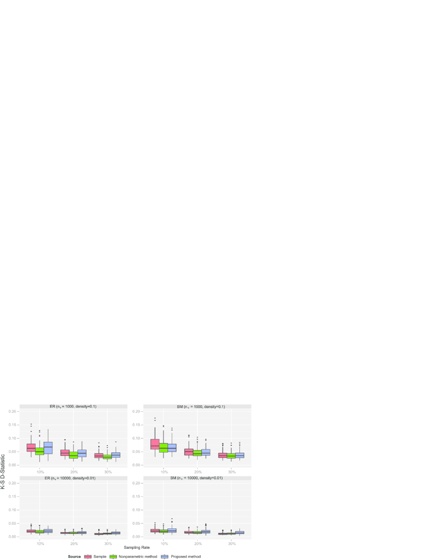
Figure 7: Simulation results for ego-centric sampling. Error measured by K–S D-statistic. For each sampling rate, the three boxes from left to right represent K–S D-statistic comparing the true degree distribution with (left) sample degree distribution, (middle) estimated degree distribution using the nonparametric method and (right) estimated degree distribution using the proposed method. (Online versions of the figure are in color.)

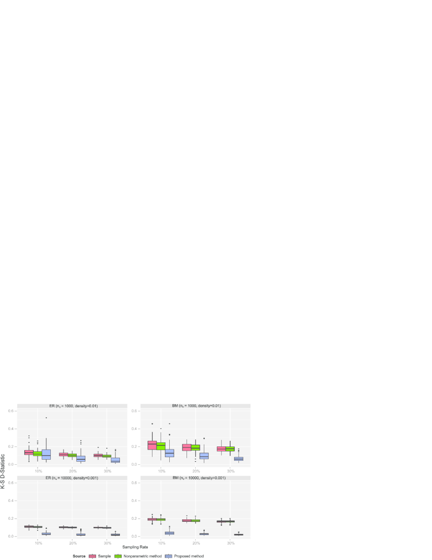
Figure 8: Simulation results for one-wave snowball sampling. Error measured by K–S D-statistic. For each sampling rate, the three boxes from left to right represent K–S D-statistic comparing the true degree distribution with (left) sample degree distribution, (middle) estimated degree distribution using the nonparametric method and (right) estimated degree distribution using the proposed method. (Online versions of the figure are in color.)

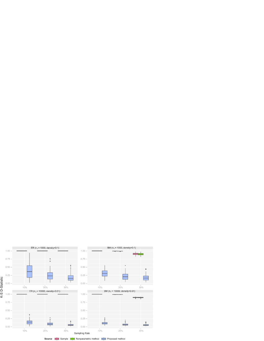
Figure 9: Simulation results for induced subgraph sampling. Error measured by K–S D-statistic. For each sampling rate, the three boxes from left to right represent K–S D-statistic comparing the true degree distribution with (left) sample degree distribution, (middle) estimated degree distribution using the nonparametric method and (right) estimated degree distribution using the proposed method. (Online versions of the figure are in color.) (Note: Only the performance of the proposed estimator $\hat{N}$ avoids the extremes of 1.0 in most cases.)

Notice that the scale of Figure 7 is from $0$ to $0.2$, much smaller than that of Figure 8 which is from $0$ to $0.6$, and Figure 9 which is from $0$ to $1$. The scales of the K–S D-statistics match the difficulty of the inverse problems they come from, with ego-centric sampling yielding an easier problem than one-wave snowball and induced subgraph sampling, as was discussed in Section 2. We compare the estimated degree distributions from our method with the sample degree distributions and the estimates from a standard kernel-smoothing method [Dong and Simonoff (1994)] described in Section 3.3. Only in the case of ego-centric sampling, the sample degree distribution and the kernel-smoothing method are competitive with our method. For one-wave snowball and induced subgraph sampling, our method yields much better results than the sample and kernel-smoothing method. This is to be expected, of course, since the kernel-smoothing method does not account for the underlying inverse problem.

In Figures 7–9, the performance in the second row is better than the performance in the first row in general. That is, performance improves with larger networks of lower density, given fixed average degree. There are three reasons for this phenomenon. First, in the standard Erdös–Rényi model, as $n_{v}$ grows to infinity and the density shrinks to zero, while the average degree is fixed, the degree distribution becomes smoother and reaches a Poisson distribution in the limit. Second, as density shrinks and $n_{v}$ grows, the normal/Poisson approximation of $N_{k}^{*}$, for $k=0,1,\ldots,M$, is better. And, in turn, the approximation of covariance matrix $C$ is more accurate.

Comparing Erdös–Rényi and the block model under the induced subgraph sampling (Figure 9), the block model has a broader range of degrees than the Erdös–Rényi model at any given choice of our other simulation parameters. In (14), for each $k$, the indicator function involving $u\in V$ with higher $d_{u}$ has lower probability of being equal to $1$. Thus, a better Poisson approximation of $N_{k}^{*}$ and a more accurate approximation of $C$ occur under the block model. A power-law network has an even broader degree distribution. For the same reasons, therefore, we expect the estimators for the power-law like networks in the applications of Section 5 to perform similarly well. However, the results for Erdös–Rényi and the block model are quite close in Figures 7 and 8. This is because only the vertex with degree $k$ in the true network can possibly contribute to degree $k$ under ego-centric and one-wave snowball sampling.

Three sampling rates are studied: 10%, 20%, and 30%. Our results show that there is less accuracy for smaller sampling rate, as is to be expected. In the literature on Internet community monitoring, 30% sampling rates have been suggested as reasonable for preserving network properties to a reasonable accuracy [Leskovec and Faloutsos (2006)]. In our results, we see that our estimators of degree distribution perform fairly well based on as low as a 10% sampling rate.

5 Applications

The cost of any sampling strategy varies with the structure of the network and the protocol. As we have remarked, sampling is of particular interest in the context of online social networks. In online social networks where each user is assigned a unique user id, it is a common practice to select a set of users by querying a set of randomly generated user id’s [Ribeiro and Towsley (2010)]. Thus, our induced subgraph sampling can be applied there. In this section, we use our degree distribution estimation method on data from three online social networks: Friendster, Orkut and LiveJournal. These data are available on the SNAP (Stanford Network Analysis Project) website. In the following we present our estimates of various degree distributions from these online social networks. In addition, we show how these degree distributions help us to gain insight about the epidemic thresholds of these networks, which is relevant to the concept of social influence, spread of rumors and viral marketing.

5.1 Estimating degree distributions from online social networks

It is now well understood that large-scale, real-world networks frequently have heavy-tailed degree distributions. Stumpf and Wiuf (2005) proved analytically that for a network with an exact power-law degree distribution, although its sampled network under our sampling method [induced Subgraph sampling with $\operatorname{Bernoulli}(p)$ for selecting vertices] is not an exact power-law network, the degree distribution for large enough degrees is power law and has the same exponent with the true network. In reality, however, most networks with heavy-tailed degree distribution will not have an exact power law. Many, for example, exhibit exponential-like deviation from a power law after some cutoff. As a result, the result of Stumpf and Wiuf (2005) does not hold in such situations and estimation is therefore still of fundamental interest.

In addition, the full Friendster, Orkut and LiveJournal networks arguably are of less interest here, being a rather coarse-grained aggregation of much finer-scale social interactions. Accordingly, we focus instead on the estimation of degree distributions for subnetworks corresponding to certain communities within these networks. In these online social networks, users create functional groups that others can join, based on, for example, topics, shared interests and hobbies, or geographical regions. In our application, we use ground-truth communities established by Yang and Leskovec (2012). For example, these authors found that LiveJournal categorizes social groups into the categories of “culture, entertainment, expression, fandom, gaming, life/style, life/support, sports, student life and technology” [Yang and Leskovec (2012)]. It is the degree distributions for subnetworks corresponding to collections of ground-truth communities such as these that we estimate here.

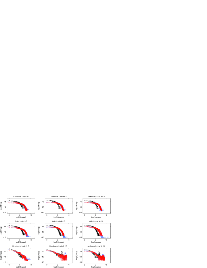
Figure 10: Estimating degree distributions of communities from Friendster, Orkut and LiveJournal. Squares represent the true degree distributions, stars represent the sample degree distributions, and triangles represent the estimated degree distributions. Sampling rate $=$ 30%. Points which correspond to a density${}<10^{-4}$ are eliminated from the plot. (Online versions of the figure are in color.)

1

Figure 10 gives an example of the estimators. The first row is for three subnetworks from Friendster. Communities are ordered according to the number of users in them. In the top left subplot, vertices from the top 5 communities form an induced subnetwork for which the degree distribution is to be estimated. Then Bernoulli sampling of vertices with $30\%$ sampling rate is performed on this subnetwork, and our estimation method is applied. Similarly, the true network in the top middle plot is induced by the top 6–15 communities, and in the top right plot the true network is induced by the top 16–30 communities. The second row and the third row show estimates of Orkut and LiveJournal, respectively. Examination of these plots shows that, while the sampled degree distribution can be quite off from the truth, particularly in the case of the Friendster and Orkut networks, correction for sampling using our proposed methodology results in estimates that are nearly indistinguishable by eye from the true degree distributions.

In Table 1 the median and inter-quartile range are computed based on the application of our estimator to 20 samples. The estimated degree distribution greatly improves over the degree distribution of the sample, as measured by the K–S D-statistic. In fact, the improvement in accuracy is by an order of magnitude, with the values of the D-statistic produced by our estimator being on the same order of magnitude as the best results in our simulation study.

= Sample Estimator Numbers of vertices Numbers of edges D-statistic D-statistic Net cmty dmax Median IQR Median IQR 01–50 0,5748 163,888 0494 0.4242 0.0196 0.0221 0.0080 Friendster 06–15 0,6385 131,875 0383 0.4521 0.0164 0.0187 0.0107 16–30 0,7097 162,616 0357 0.4813 0.0211 0.0143 0.0161 01–50 22,059 689,659 0895 0.4092 0.0145 0.0134 0.0073 Orkut 06–15 29,681 591,448 0578 0.4322 0.0129 0.0099 0.0059 16–30 31,018 619,909 1779 0.4324 0.0068 0.0175 0.0076 01–50 0,5131 085,419 0801 0.3018 0.0285 0.0430 0.0258 LiveJournal 06–15 0,3757 219,193 0547 0.2678 0.0153 0.0558 0.0105 16–30 0,4591 228,633 0512 0.2941 0.0137 0.0643 0.0404

Table 1: Network communities summary. Each median and inter-quartile range is computed based on the application of our estimator to 20 samples

In summary, our method of estimating the degree distribution from sampled networks clearly can offer substantial advantages over raw measured networks in monitoring the degree distribution of the communities in online social networks. This provides a powerful additional motivation for using sampling in these contexts.

5.2 Characterizing epidemic spread

In this subsection we are going to show how recovery of the degree distribution—as a fundamental object—helps for monitoring other socially pertinent questions, for example, characterizing epidemic spread on networks.

As has been shown by various authors [e.g., Bailey et al. (1975), Daley and Gani (1999), Kephart and White (1991), Pastor-Satorras and Vespignani (2001)], an epidemic threshold $\tau_{c}$ exists in a virus spread in networks. Under a standard Susceptible–Infected–Susceptible (SIS) model, let the infection rate be $\beta$ and the curing rate be $\delta$. If the effective spreading rate $\tau=(\beta/\delta)>\tau_{c}$, the virus persists and a nonzero fraction of the nodes are infected, whereas for $\tau\leq\tau_{c}$ the epidemic dies out. This threshold is shown to equal the inverse of the largest eigenvalue $\lambda_{1}$ of the network’s adjacency matrix in Van Mieghem, Omic and Kooij (2009).

The degree distribution of a network can be used to get bounds for the largest eigenvalue $\lambda_{1}$ of the adjacency matrix, and thus bounds for $1/\lambda_{1}$. Let $M_{1}$ be the first raw moment of the degree distribution, that is, the average degree, $M_{2}$ be the second raw moment of the degree distribution, $n_{e}=|E|$ be the number of total edges, and $U=(2*n_{e}(n_{v}-1)/n_{v})^{1/2}$. Then we have the following relationship:

$$M_{1}\leq\sqrt{M_{2}}\leq\lambda_{1}\leq U.$$ (22)

The proof of the first two inequalities can be found in Van Mieghem (2011), and the third (upper bound) can be found in Lovász (1993). Thus, we have the bounds for the epidemic threshold $\tau_{c}$,

$$1/U\leq\tau_{c}\leq\frac{1}{\sqrt{M}_{2}}\leq\frac{1}{M_{1}}.$$ (23)

Figures 11–13 show the bounds obtained from the estimated degree distribution and those obtained from the original sample degree distribution. The networks used are the online social networks described in Section 5.1. It can be seen from Figures 11–13 that our method estimates the bounds with high accuracy, whereas the bounds using the sampled data are way off.

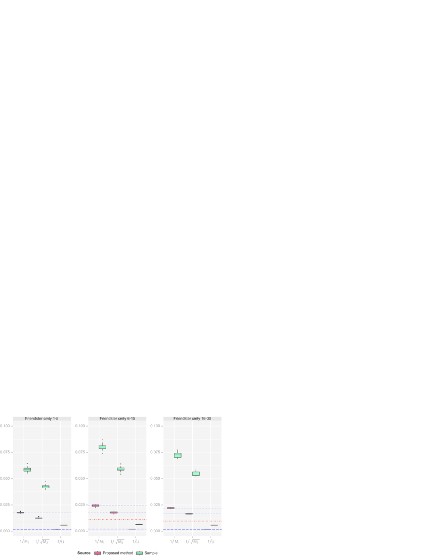
Figure 11: Bounds for the epidemic spreads of Friendster networks, each box is estimated based on 20 samples, four horizontal lines are the true values for $\frac{1}{M_{1}}$, $\frac{1}{\sqrt{M_{2}}}$, $\frac{1}{\lambda_{1}}$ and $\frac{1}{U}$ from top to bottom. For each bound, the two boxes from left to right correspond to the estimated value using (left) the proposed method and (right) the sample degree distribution. (Online versions of the figure are in color.)

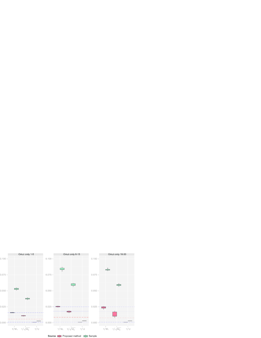
Figure 12: Bounds for the epidemic spreads of Orkut networks, each box is estimated based on 20 samples, four horizontal lines are the true values for $\frac{1}{M_{1}}$, $\frac{1}{\sqrt{M_{2}}}$, $\frac{1}{\lambda_{1}}$ and $\frac{1}{U}$ from top to bottom. For each bound, the two boxes from left to right correspond to the estimated value using (left) the proposed method and (right) the sample degree distribution. (Online versions of the figure are in color.)

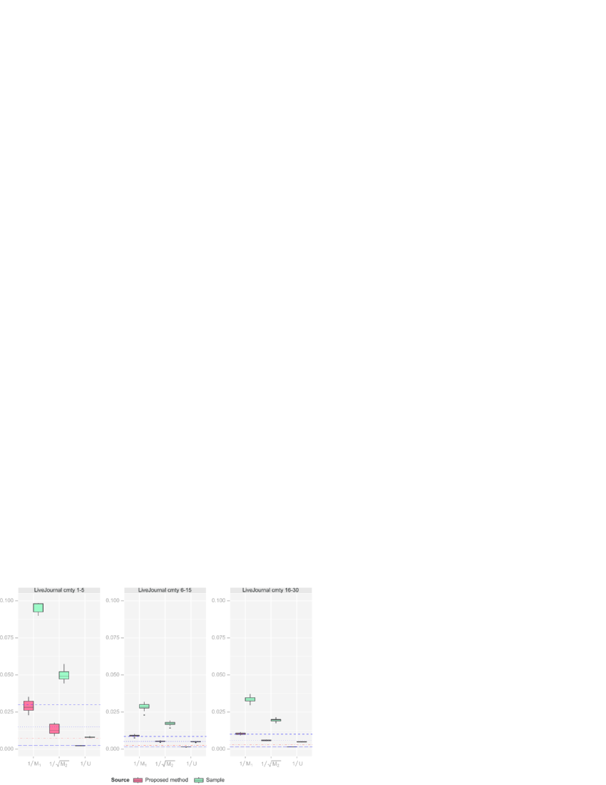
Figure 13: Bounds for the epidemic spreads of LiveJournal networks, each box is estimated based on 20 samples, four horizontal lines are the true values for $\frac{1}{M_{1}}$, $\frac{1}{\sqrt{M_{2}}}$, $\frac{1}{\lambda_{1}}$ and $\frac{1}{U}$ from top to bottom. For each bound, the two boxes from left to right correspond to the estimated value using (left) the proposed method and (right) the sample degree distribution. (Online versions of the figure are in color.)

Since our estimator successfully recovers the degree distribution of the online social networks, the epidemic threshold (the inverse of the spectral radius) of the network can be successfully bounded by functions of our estimates. This has important implications in practical applications. For example, in viral marketing, the epidemic threshold relates to how hard a company’s marketing force needs to work, that is, it is necessary for them to make the effective spreading rate $\tau$ as large as $1/U$, and sufficient to make $\tau$ as large as $\frac{1}{\sqrt{M}_{2}}$, in order to make a product’s advertisement remembered by people in the network.

6 Discussion

The problem of estimating the degree distribution of a network from a sampled subnetwork was first posed by Ove Frank in his 1971 Ph.D. dissertation [Frank (1971)]. In the ensuing years, the problem appears to have received very little attention, likely in no small part to its apparent difficulty. Here we recast the original problem as a linear inverse problem. We have demonstrated that, in so doing, it is possible to obtain substantial insight into the inherent difficulty of the problem—in terms of the operator corresponding to the sampling, the nature of the “noise” induced by the sampling and the manner in which the two interact. Leveraging this insight, we have proposed a penalized, generalized least squares estimator, with positivity constraints, that solves our linear inverse problem. The choice of smoothing parameter is nontrivial in this context and we offer a Monte Carlo approach to optimizing a generalized SURE criterion as an effective option. Finally, our simulations and application to online social media networks show that the methodology can perform quite well under a variety of choices of network topology—even under sampling rates as low as 10%.

There are a number of directions upon which to build from the work we present here. The assumptions discussed in Section 2.4 could be relaxed, for example, to include observation errors, to incorporate estimates of possible unknown parameters in the matrix $P$, or to focus on matrices $P$ which depend on the network $G$ itself. In this case, a model-based framework is likely necessary, and for that it would be natural to try to integrate our framework with the work of Handcock and Gile (2010). Finally, another interesting direction would be developing methods for correcting the sampling bias of the degree distribution under more complex adaptive designs.

Appendix A Eigenvalue decomposition

Theorem 1.

Let $P=P_{\mathrm{ind}}=\tilde{U}\Lambda\tilde{U}^{-1}$, where $\Lambda=\operatorname{diag}(\lambda_{1},\ldots,\lambda_{M+1})$ is a diagonal matrix and $\tilde{U}=(\tilde{\mathbf{u}}_{1},\tilde{\mathbf{u}}_{2},\ldots,\tilde{\mathbf{u}}_{M+1})$ is a nonsingular matrix. Then the $k$th eigenvalue $\lambda_{k}$ and eigenvector $\tilde{u}_{k}$ of $P$ are

$$\lambda_{k} = p^{k},$$ (24)

$$\tilde{\mathbf{u}}_{k}(j) = \cases{\displaystyle(-1)^{k-j}\pmatrix{k-1\cr j-1},&$\quad\mbox{for }1\leq j\leq k$,\vspace*{3pt}\cr 0,&\quad$\mbox{for }k<j\leq M+1$.}$$ (25)

We will prove this theorem by induction. In the case that $P$ is a $2$ by $2$ matrix,

$$P=\left[\matrix{p&pq\vspace*{2pt}\cr 0&p^{2}}\right].$$ (26)

It’s easy to show that

$$\tilde{U}=\left[\matrix{1&0\vspace*{2pt}\cr-1&0}\right].$$ (27)

The theorem is true if $P$ is a $2$ by $2$ matrix. Suppose it is true when $P$ is a $k-1$ by $k-1$ matrix, then in the case that $P$ is $k$ by $k$,

$$\qquad{{P=\left[\matrix{\ddots&&&&\vspace*{3pt}\cr&p^{k-3}&\pmatrix{k-3\cr 1}p^{k-3}q&\pmatrix{k-2\cr 2}p^{k-3}q^{2}&\pmatrix{k-1\cr 3}p^{k-3}q^{3}\vspace*{4pt}\cr&0&p^{k-2}&\pmatrix{k-2\cr 1}p^{k-2}q&\pmatrix{k-1\cr 2}p^{k-2}q^{2}\vspace*{4pt}\cr&0&0&p^{k-1}&\pmatrix{k-1\cr 1}p^{k-1}q\vspace*{4pt}\cr&0&0&0&p^{k}}\right].}}$$ (28)

Because of the upper-triangular nature of the matrix, the first $k-1$ entries in each of the first $k-1$ eigenvectors are the same as in the case that $P$ is $k-1$ by $k-1$, and the $k$th entry is filled with zero.

For eigenvalue $\lambda_{k}=p_{k}$, let $\mathbf{x}=(x_{1},x_{2},\ldots,x_{k})^{T}$ and $x_{k}=1$ be the solution of the eigenvalue equation

$$(P-\lambda_{k}I)\mathbf{x}$$

$$\qquad={{\left[\matrix{\ddots&&&&\vspace*{4pt}\cr&p^{k-3}\bigl{(}1-p^{3}\bigr{)}&\pmatrix{k-3\cr 1}p^{k-3}q&\pmatrix{k-2\cr 2}p^{k-3}q^{2}&\pmatrix{k-1\cr 3}p^{k-3}q^{3}\vspace*{4pt}\cr&0&p^{k-2}\bigl{(}1-p^{2}\bigr{)}&\pmatrix{k-2\cr 1}p^{k-2}q&\pmatrix{k-1\cr 2}p^{k-2}q^{2}\vspace*{4pt}\cr&0&0&p^{k-1}(1-p)&\pmatrix{k-1\cr 1}p^{k-1}q\vspace*{4pt}\cr&0&0&0&0}\right]}}\mathbf{x}$$ (29)

$$\qquad=0.$$

The equation at the $(k-1)$th row is

$$p^{k-1}(1-p)x_{k}+\pmatrix{k-1\cr 1}p^{k-1}qx_{k}=0.$$ (30)

We solve for $x_{k-1}$,

$$x_{k-1}=\frac{{k-1\choose 1}p^{k-1}q}{p^{k-1}(1-p)}=-\pmatrix{k-1\cr 1}.$$ (31)

Assuming $x_{k-i}=(-1)^{i}{k-1\choose i}$, for $i=0,1,\ldots,n-1$, we solve for $x_{k-n}$ from the equation at the ($k-n$)th row:

$$-p^{k-n}\bigl{(}1-p^{n}\bigr{)}x_{k-n} = \pmatrix{k-n\cr 1}p^{k-n}qx_{k-(n-1)}$$

$${}+\pmatrix{k-(n-1)\cr 2}p^{k-n}q^{2}x_{k-(n-1)}+\cdots$$

$${}+\pmatrix{k-2\cr n-1}p^{k-n}q^{n-1}x_{k-1}+\pmatrix{k-1\cr n}p^{k-n}q^{n}x_{k}.$$

Simplifying the above equation, we have

$$-\bigl{(}1-p^{n}\bigr{)}x_{k-n}$$

$$\qquad=\pmatrix{k-n\cr 1}\pmatrix{k-1\cr n-1}(-1)^{n-1}q$$

$$\qquad\quad{}+\pmatrix{k-(n-1)\cr 2}\pmatrix{k-1\cr n-2}(-1)^{n-2}q^{2}+\cdots$$

$$\qquad\quad{}+\pmatrix{k-2\cr n-1}\pmatrix{k-1\cr 1}(-1)^{1}q^{n-1}+\pmatrix{k-1\cr n}(-1)^{0}q^{n}$$

(33)

$$\qquad=(-1)^{n}\pmatrix{k-1\cr n}$$

$$\qquad\quad{}\times\biggl{[}\pmatrix{n\cr 1}(-q)+\pmatrix{n\cr 2}(-q)^{2}+\cdots+\pmatrix{n\cr 1}(-q)^{n-1}+\pmatrix{n\cr 0}(-q)^{n}\biggr{]}$$

$$\qquad=(-1)^{n}\pmatrix{k-1\cr n}\bigl{[}(1-q)^{n}-1\bigr{]}$$

$$\qquad=(-1)^{n}\pmatrix{k-1\cr n}\bigl{(}p^{n}-1\bigr{)}.$$

Finally,

$$x_{k-n}=(-1)^{n}\pmatrix{k-1\cr n}.$$ (34)

Therefore, the entries in the $k$th eigenvector are

$$\tilde{\mathbf{u}}_{k}(j)=\cases{\displaystyle(-1)^{k-j}\pmatrix{k-1\cr j-1},&\quad$\mbox{for }1\leq j\leq k$,\vspace*{3pt}\cr 0,&\quad$\mbox{for }k<j\leq M+1$.}$$ (35)

The theorem is true for $k$ by $k$ matrix $P$.

Appendix B Poisson approximation

Here we give a proof of the Poisson approximation of the cumulative degree vectors, under one-wave snowball sampling and induced subgraph sampling with $\operatorname{Bernoulli}(p)$ for selecting edges. The arguments for both designs are nearly identical, and so we present them together.

Theorem 2.

Assume $G^{*}$ is produced by induced subgraph sampling with Bernoulli sampling to select $S$. Let

$$\tilde{N}_{k}^{*}=\sum_{r=k}^{M}N_{r}^{*}=\sum_{v}I\bigl{\{}v\in S,d_{v}^{*}\geq k\bigr{\}}$$ (36)

be the number of vertices of degree $k$ or larger in $G^{*}$. Let

$$\lambda_{k}=E\bigl{(}\tilde{N}_{k}^{*}\bigr{)}=\sum_{v:d_{v}\geq k}\pi_{k,v},$$ (37)

where

$$\pi_{k,v}=P\bigl{(}v\in S,d_{v}^{*}\geq k\bigr{)}.$$ (38)

Then

$$\hskip 6.0pt\operatorname{dist}_{\mathrm{TV}}\bigl{(}\mathcal{L}\bigl{(}\tilde{N}_{k}^{*}\bigr{)},\operatorname{Po}(\lambda_{k})\bigr{)}\leq\frac{1-e^{-\lambda_{k}}}{\lambda_{k}}\biggl{[}\operatorname{Var}\bigl{(}\tilde{N}_{k}^{*}\bigr{)}-\lambda_{k}+2\sum_{v\dvtx d_{v}\geq k}\pi_{k,v}^{2}\biggr{]},$$ (39)

where $\operatorname{dist}_{\mathrm{TV}}$ indicates the total-variation distance between its arguments, $\mathcal{L}$ means “law of,” and $\operatorname{Po}(\lambda_{k})$ is a Poisson random variable with intensity $\lambda_{k}$.

We sketch the proof briefly here. Without loss of generality, (partially) order the vertices $\{v_{1},\ldots,v_{n_{v}}\}$ by (non)decreasing degree. Associate a binary random vector $(X_{1},\ldots,X_{n_{v}})$ with the vertices, where the elements are independent Bernoulli random variables with parameter $p$. So $\mathbf{X}$ represents the selection of vertices for inclusion in $S$ in the case of induced subgraph sampling and the initial selection of vertices in the case of snowball sampling. Now let $I_{v,k}$ be an indicator random variable, which is one if $v\in S$ and $d_{v}^{*}\geq k$. Then the variables $I_{v,k}$ are so-called “increasing functions” of realizations of $X$. So Corollary 2.E.1, page 28, of Poisson Approximation, by Barbour and colleagues, yields our result.

In more detail, there are two key observations to be made. First, we need the $I_{v,k}$ to be increasing functions. This induces positive correlation among these indicator variables and it makes a general Chen–Stein bound become much cleaner, as in our theorem, in that it can be expressed explicitly in terms of means and variances. Partial ordering means that if we let $\mathbf{x}$ and $\mathbf{y}$ be two possible realizations of $\mathbf{X}$, then $\mathbf{x}\leq\mathbf{y}$ if and only if $x_{i}\leq y_{i}$ for all $i$. And a function $f$ is increasing if $f(\mathbf{x})\leq f(\mathbf{y})$ whenever $\mathbf{x}\leq\mathbf{y}$. For $\mathbf{x}$ to be less than or equal to $\mathbf{y}$, it suffices to think of what happens simply when a new vertex enters the sample $S$. One element of $\mathbf{x}$ will change from a zero to a one, so $\mathbf{x}\leq\mathbf{y}$. What happens to $I_{v,k}$? If $v$ is a vertex that was already in $S$, under $x$, then adding a vertex to the sample under $\mathbf{y}$ can either not change or increase its degree. So $I_{v,k}(\mathbf{x})\leq I_{v,k}(\mathbf{y})$. On the other hand, if $v$ itself was the new vertex to enter $S$ under $y$, the same statement can be made.

Second is the observation that elements of $\mathbf{X}$ are independent in our setting, which is guaranteed by our assumption of Bernoulli sampling. Taken together, these two things mean that Theorem 2.E holds in Barbour et al., that is, positive dependence. And so Corollary 2.E.1 holds and we have our result.

Appendix C Conditions to use generalized SURE

C.1 Weak differentiability of $f_{\lambda}(\mathbf{N}^{*})$

Let’s first ignore the nonnegativity constraints. Then 16 becomes

$$\mathop{\mbox{minimize}}_{N}\qquad\bigl{(}P\mathbf{N}-\mathbf{N}^{*}\bigr{)}^{T}C^{-1}\bigl{(}P\mathbf{N}-\mathbf{N}^{*}\bigr{)}+\lambda\cdot\operatorname{penalty}\bigl{(}\mathbf{N}^{*}\bigr{)}$$

(40)

$$\mbox{subject to}\qquad\sum_{i=0}^{M}{N_{i}}=n_{v}.$$

The Lagrange function is

$$L=\bigl{(}\mathbf{N}^{*}-P\mathbf{N}\bigr{)}^{T}\bigl{(}\mathbf{N}^{*}-P\mathbf{N}\bigr{)}+\lambda\mathbf{N}^{T}\Omega\mathbf{N}+\alpha\bigl{(}\mathbf{1}^{T}\mathbf{N}-n_{v}\bigr{)}.$$ (41)

KKT conditions:

$$\frac{dL}{d\mathbf{N}} = -2\mathbf{N}^{*T}C^{-1}P+2\mathbf{N}^{T}P^{T}C^{-1}P+2\lambda\mathbf{N}^{T}\Omega+\alpha\mathbf{1}^{T}=0,$$ (42)

$$\mathbf{1}^{T}\mathbf{N} = n_{v}.$$ (43)

Then $\hat{N}$ is the solution of the following system:

$$\left[\matrix{P^{T}C^{-1}P+\lambda\Omega&\tfrac{1}{2}\mathbf{1}\vspace*{3pt}\cr\mathbf{1}^{T}&0}\right]\left[\matrix{\mathbf{N}\cr\alpha}\right]=\left[\matrix{2P^{T}C^{-1}\mathbf{N}^{*}\vspace*{2pt}\cr n_{v}}\right].$$ (44)

Let $A=P^{T}C^{-1}P+\lambda\Omega$ and $B=\bigl{[}{{\matrix{A&\tfrac{1}{2}\mathbf{1}\vspace*{-0.5pt}\cr\mathbf{1}^{T}&0}}}\bigr{]}$. Since both $A$ and $\mathbf{1}^{T}A^{-1}\mathbf{1}$ are invertible for sufficiently large $\lambda$, $B$ is invertible:

$$\hat{\mathbf{N}}=B^{-1}P^{T}C^{-1}\mathbf{N}^{*}=\sum_{i=0}^{M}d_{i}\bigl{(}\mathbf{u}_{i}^{T}C^{-1}\mathbf{N}^{*}\bigr{)}B^{-1}\mathbf{v}_{i}.$$ (45)

Thus, $\hat{\mathbf{N}}$ is a linear function of the observed $\mathbf{N}^{*}$. In this case, $f_{\lambda}(\mathbf{N}^{*})$ is differentiable w.r.t. $\mathbf{N}^{*}$.

Adding nonnegativity constraints only gives nondifferentiable points at the boundary, so the set of nondifferentiable points has measure zero. $f_{\lambda}(\mathbf{N}^{*})$ has a derivative almost everywhere. $f_{\lambda}(\mathbf{N}^{*})$ is weakly differentiable.

C.2 $E\{|f_{\lambda}(\mathbf{N}^{*})|\}$ is bounded

Assuming $\mathbf{N}^{*}$ is Gaussian, since $f_{\lambda}(\mathbf{N}^{*})$ is a linear function of $\mathbf{N}^{*}$ within the feasible set of $\hat{\mathbf{N}}$, $f_{\lambda}(\mathbf{N}^{*})$ is also Gaussian, thus $E\{|f_{\lambda}(\mathbf{N}^{*})|\}$ is bounded.

References

- Achlioptas et al. (2005) {bincollection}[mr] \bauthor\bsnmAchlioptas, \bfnmDimitris\binitsD., \bauthor\bsnmClauset, \bfnmAaron\binitsA., \bauthor\bsnmKempe, \bfnmDavid\binitsD. and \bauthor\bsnmMoore, \bfnmCristopher\binitsC. (\byear2005). \btitleOn the bias of traceroute sampling or, power-law degree distributions in regular graphs. In \bbooktitleSTOC’05: Proceedings of the 37th Annual ACM Symposium on Theory of Computing \bpages694–703. \bpublisherACM, \blocationNew York. \biddoi=10.1145/1060590.1060693, mr=2181674 \bptokimsref\endbibitem
- Ahmed, Neville and Kompella (2011) {bmisc}[author] \bauthor\bsnmAhmed, \bfnmNesreen\binitsN., \bauthor\bsnmNeville, \bfnmJennifer\binitsJ. and \bauthor\bsnmKompella, \bfnmRamana Rao\binitsR. R. (\byear2011). \bhowpublishedNetwork sampling via edge-based node selection with graph induction. CSD TR # 11-016 1–10. Purdue Univ., West Lafayette, IN. \bptokimsref\endbibitem
- Ahmed, Neville and Kompella (2012) {binproceedings}[author] \bauthor\bsnmAhmed, \bfnmNesreen K.\binitsN. K., \bauthor\bsnmNeville, \bfnmJennifer\binitsJ. and \bauthor\bsnmKompella, \bfnmRamana Rao\binitsR. R. (\byear2012). \btitleNetwork sampling designs for relational classification. In \bbooktitleICWSM. \bptokimsref\endbibitem
- Ahmed et al. (2010) {binproceedings}[author] \bauthor\bsnmAhmed, \bfnmNesreen K.\binitsN. K., \bauthor\bsnmBerchmans, \bfnmFredrick\binitsF., \bauthor\bsnmNeville, \bfnmJennifer\binitsJ. and \bauthor\bsnmKompella, \bfnmRamana\binitsR. (\byear2010). \btitleTime-based sampling of social network activity graphs. In \bbooktitleProceedings of the Eighth Workshop on Mining and Learning with Graphs \bpages1–9. \bpublisherACM, \blocationNew York. \bptokimsref\endbibitem
- Ahn et al. (2007) {binproceedings}[author] \bauthor\bsnmAhn, \bfnmYong-Yeol\binitsY.-Y., \bauthor\bsnmHan, \bfnmSeungyeop\binitsS., \bauthor\bsnmKwak, \bfnmHaewoon\binitsH., \bauthor\bsnmMoon, \bfnmSue\binitsS. and \bauthor\bsnmJeong, \bfnmHawoong\binitsH. (\byear2007). \btitleAnalysis of topological characteristics of huge online social networking services. In \bbooktitleProceedings of the 16th International Conference on World Wide Web \bpages835–844. \bpublisherACM, \blocationNew York. \bptokimsref\endbibitem
- Bailey et al. (1975) {bbook}[author] \bauthor\bsnmBailey, \bfnmNorman TJ\binitsN. T. \betalet al. (\byear1975). \btitleThe Mathematical Theory of Infectious Diseases and Its Applications. \bpublisherCharles Griffin & Company Ltd., \blocationLondon. \bptokimsref\endbibitem
- Boyd and Vandenberghe (2004) {bbook}[mr] \bauthor\bsnmBoyd, \bfnmStephen\binitsS. and \bauthor\bsnmVandenberghe, \bfnmLieven\binitsL. (\byear2004). \btitleConvex Optimization. \bpublisherCambridge Univ. Press, \blocationCambridge. \biddoi=10.1017/CBO9780511804441, mr=2061575 \bptokimsref\endbibitem
- Cochran (1977) {bbook}[mr] \bauthor\bsnmCochran, \bfnmWilliam G.\binitsW. G. (\byear1977). \btitleSampling Techniques, \bedition3rd ed. \bpublisherWiley, \blocationNew York. \bidmr=0474575 \bptokimsref\endbibitem
- CVX Research (2012) {bmisc}[author] \bauthor\bsnmCVX Research, \bfnmInc.\binitsInc. (\byear2012). \bhowpublishedCVX: Matlab software for disciplined convex programming, version 2.0 beta. Available at: \surlhttp://cvxr.com/cvx. \bptokimsref\endbibitem
- Daley and Gani (1999) {bmisc}[author] \bauthor\bsnmDaley, \bfnmD. J.\binitsD. J. and \bauthor\bsnmGani, \bfnmJ. M.\binitsJ. M. (\byear1999). \bhowpublishedEpidemic Modelling: An Introduction. Cambridge Univ. Press, Cambridge. \bptokimsref\endbibitem
- Dong and Simonoff (1994) {barticle}[author] \bauthor\bsnmDong, \bfnmJianping\binitsJ. and \bauthor\bsnmSimonoff, \bfnmJeffrey S.\binitsJ. S. (\byear1994). \btitleThe construction and properties of boundary kernels for smoothing sparse multinomials. \bjournalJ. Comput. Graph. Statist. \bvolume3 \bpages57–66. \bptokimsref\endbibitem
- Eldar (2009) {barticle}[mr] \bauthor\bsnmEldar, \bfnmYonina C.\binitsY. C. (\byear2009). \btitleGeneralized SURE for exponential families: Applications to regularization. \bjournalIEEE Trans. Signal Process. \bvolume57 \bpages471–481. \biddoi=10.1109/TSP.2008.2008212, issn=1053-587X, mr=2603376 \bptokimsref\endbibitem
- Frank (1971) {bmisc}[author] \bauthor\bsnmFrank, \bfnmOve\binitsO. (\byear1971). \bhowpublishedStatistical inference in graphs. Ph.D. thesis, Foa Repro Stockholm. \bptokimsref\endbibitem
- Frank (1980) {barticle}[mr] \bauthor\bsnmFrank, \bfnmOve\binitsO. (\byear1980). \btitleEstimation of the number of vertices of different degrees in a graph. \bjournalJ. Statist. Plann. Inference \bvolume4 \bpages45–50. \biddoi=10.1016/0378-3758(80)90032-4, issn=0378-3758, mr=0587030 \bptokimsref\endbibitem
- Frank (1981) {barticle}[author] \bauthor\bsnmFrank, \bfnmOve\binitsO. (\byear1981). \btitleA survey of statistical methods for graph analysis. \bjournalSociol. Method. \bvolume12 \bpages110–155. \bptokimsref\endbibitem
- Frank (2005) {binproceedings}[author] \bauthor\bsnmFrank, \bfnmOve\binitsO. (\byear2005). \btitleNetwork sampling and model fitting. In \bbooktitleModels and Methods in Social Network Analysis \bpages31–56. \bpublisherCambridge Univ. Press, \blocationCambridge. \bptokimsref\endbibitem
- Gjoka et al. (2010) {binproceedings}[author] \bauthor\bsnmGjoka, \bfnmMinas\binitsM., \bauthor\bsnmKurant, \bfnmMaciej\binitsM., \bauthor\bsnmButts, \bfnmCarter T.\binitsC. T. and \bauthor\bsnmMarkopoulou, \bfnmAthina\binitsA. (\byear2010). \btitleWalking in Facebook: A case study of unbiased sampling of OSNs. In \bbooktitleINFOCOM, 2010 Proceedings IEEE \bpages1–9. \bpublisherIEEE, \blocationNew York. \bptokimsref\endbibitem
- Gjoka et al. (2011) {barticle}[author] \bauthor\bsnmGjoka, \bfnmMinas\binitsM., \bauthor\bsnmButts, \bfnmCarter T.\binitsC. T., \bauthor\bsnmKurant, \bfnmMaciej\binitsM. and \bauthor\bsnmMarkopoulou, \bfnmAthina\binitsA. (\byear2011). \btitleMultigraph sampling of online social networks. \bjournalIEEE J. Sel. Areas Commun. \bvolume29 \bpages1893–1905. \bptokimsref\endbibitem
- Hall and Titterington (1987) {barticle}[mr] \bauthor\bsnmHall, \bfnmPeter\binitsP. and \bauthor\bsnmTitterington, \bfnmD. M.\binitsD. M. (\byear1987). \btitleOn smoothing sparse multinomial data. \bjournalAust. J. Stat. \bvolume29 \bpages19–37. \bidissn=0004-9581, mr=0899373 \bptokimsref\endbibitem
- Handcock and Gile (2010) {barticle}[mr] \bauthor\bsnmHandcock, \bfnmMark S.\binitsM. S. and \bauthor\bsnmGile, \bfnmKrista J.\binitsK. J. (\byear2010). \btitleModeling social networks from sampled data. \bjournalAnn. Appl. Stat. \bvolume4 \bpages5–25. \biddoi=10.1214/08-AOAS221, issn=1932-6157, mr=2758082 \bptokimsref\endbibitem
- Hubler et al. (2008) {binproceedings}[author] \bauthor\bsnmHubler, \bfnmChristian\binitsC., \bauthor\bsnmKriegel, \bfnmH.-P.\binitsH.-P., \bauthor\bsnmBorgwardt, \bfnmKarsten\binitsK. and \bauthor\bsnmGhahramani, \bfnmZoubin\binitsZ. (\byear2008). \btitleMetropolis algorithms for representative subgraph sampling. In \bbooktitleData Mining, 2008. ICDM’08. Eighth IEEE International Conference on \bpages283–292. \bpublisherIEEE, \blocationNew York. \bptokimsref\endbibitem
- Jin et al. (2011) {binproceedings}[author] \bauthor\bsnmJin, \bfnmLong\binitsL., \bauthor\bsnmChen, \bfnmYang\binitsY., \bauthor\bsnmHui, \bfnmPan\binitsP., \bauthor\bsnmDing, \bfnmCong\binitsC., \bauthor\bsnmWang, \bfnmTianyi\binitsT., \bauthor\bsnmVasilakos, \bfnmAthanasios V.\binitsA. V., \bauthor\bsnmDeng, \bfnmBeixing\binitsB. and \bauthor\bsnmLi, \bfnmXing\binitsX. (\byear2011). \btitleAlbatross sampling: Robust and effective hybrid vertex sampling for social graphs. In \bbooktitleProceedings of the 3rd ACM International Workshop on MobiArch \bpages11–16. \bpublisherACM, \blocationNew York. \bptokimsref\endbibitem
- Kephart and White (1991) {binproceedings}[author] \bauthor\bsnmKephart, \bfnmJeffrey O.\binitsJ. O. and \bauthor\bsnmWhite, \bfnmSteve R.\binitsS. R. (\byear1991). \btitleDirected-graph epidemiological models of computer viruses. In \bbooktitleResearch in Security and Privacy, 1991. Proceedings, 1991 IEEE Computer Society Symposium on \bpages343–359. \bpublisherIEEE, \blocationNew York. \bptokimsref\endbibitem
- Kolaczyk (2009) {bbook}[mr] \bauthor\bsnmKolaczyk, \bfnmEric D.\binitsE. D. (\byear2009). \btitleStatistical Analysis of Network Data: Methods and Models. \bpublisherSpringer, \blocationNew York. \biddoi=10.1007/978-0-387-88146-1, mr=2724362 \bptokimsref\endbibitem
- Kurant, Markopoulou and Thiran (2011) {barticle}[author] \bauthor\bsnmKurant, \bfnmMaciej\binitsM., \bauthor\bsnmMarkopoulou, \bfnmAthina\binitsA. and \bauthor\bsnmThiran, \bfnmPatrick\binitsP. (\byear2011). \btitleTowards unbiased BFS sampling. \bjournalIEEE J. Sel. Areas Commun. \bvolume29 \bpages1799–1809. \bptokimsref\endbibitem
- Kurant et al. (2011) {binproceedings}[author] \bauthor\bsnmKurant, \bfnmMaciej\binitsM., \bauthor\bsnmGjoka, \bfnmMinas\binitsM., \bauthor\bsnmButts, \bfnmCarter T.\binitsC. T. and \bauthor\bsnmMarkopoulou, \bfnmAthina\binitsA. (\byear2011). \btitleWalking on a graph with a magnifying glass: Stratified sampling via weighted random walks. In \bbooktitleProceedings of the ACM SIGMETRICS Joint International Conference on Measurement and Modeling of Computer Systems \bpages281–292. \bpublisherACM, \blocationNew York. \bptokimsref\endbibitem
- Kurant et al. (2012) {binproceedings}[author] \bauthor\bsnmKurant, \bfnmMaciej\binitsM., \bauthor\bsnmGjoka, \bfnmMinas\binitsM., \bauthor\bsnmWang, \bfnmYan\binitsY., \bauthor\bsnmAlmquist, \bfnmZack W.\binitsZ. W., \bauthor\bsnmButts, \bfnmCarter T.\binitsC. T. and \bauthor\bsnmMarkopoulou, \bfnmAthina\binitsA. (\byear2012). \btitleCoarse-grained topology estimation via graph sampling. In \bbooktitleProceedings of the 2012 ACM Workshop on Workshop on Online Social Networks \bpages25–30. \bpublisherACM, \blocationNew York. \bptokimsref\endbibitem
- Lakhina et al. (2003) {binproceedings}[author] \bauthor\bsnmLakhina, \bfnmAnukool\binitsA., \bauthor\bsnmByers, \bfnmJohn W.\binitsJ. W., \bauthor\bsnmCrovella, \bfnmMark\binitsM. and \bauthor\bsnmXie, \bfnmPeng\binitsP. (\byear2003). \btitleSampling biases in IP topology measurements. In \bbooktitleINFOCOM 2003. Twenty-Second Annual Joint Conference of the IEEE Computer and Communications. IEEE Societies \bvolume1 \bpages332–341. \bpublisherIEEE, \blocationNew York. \bptokimsref\endbibitem
- Leskovec and Faloutsos (2006) {binproceedings}[author] \bauthor\bsnmLeskovec, \bfnmJure\binitsJ. and \bauthor\bsnmFaloutsos, \bfnmChristos\binitsC. (\byear2006). \btitleSampling from large graphs. In \bbooktitleProceedings of the 12th ACM SIGKDD International Conference on Knowledge Discovery and Data Mining \bpages631–636. \bpublisherACM, \blocationNew York. \bptokimsref\endbibitem
- Li and Yeh (2011) {bincollection}[author] \bauthor\bsnmLi, \bfnmJhao-Yin\binitsJ.-Y. and \bauthor\bsnmYeh, \bfnmMi-Yen\binitsM.-Y. (\byear2011). \btitleOn sampling type distribution from heterogeneous social networks. In \bbooktitleAdvances in Knowledge Discovery and Data Mining \bpages111–122. \bpublisherSpringer, \blocationBerlin. \bptokimsref\endbibitem
- Lim et al. (2011) {binproceedings}[author] \bauthor\bsnmLim, \bfnmYeon-sup\binitsY.-s., \bauthor\bsnmMenasché, \bfnmDaniel S.\binitsD. S., \bauthor\bsnmRibeiro, \bfnmBruno\binitsB., \bauthor\bsnmTowsley, \bfnmDon\binitsD. and \bauthor\bsnmBasu, \bfnmPrithwish\binitsP. (\byear2011). \btitleOnline estimating the central nodes of a network. In \bbooktitleNetwork Science Workshop (NSW), 2011 IEEE \bpages118–122. \bpublisherIEEE, \blocationNew York. \bptokimsref\endbibitem
- Lovász (1993) {bbook}[author] \bauthor\bsnmLovász, \bfnmLászló\binitsL. (\byear1993). \btitleCombinatorial Problems and Exercises, \bedition2nd ed. \bpublisherNorth-Holland, \blocationAmsterdam. \bptokimsref\endbibitem
- Lu and Bressan (2012) {binproceedings}[author] \bauthor\bsnmLu, \bfnmXuesong\binitsX. and \bauthor\bsnmBressan, \bfnmStéphane\binitsS. (\byear2012). \btitleSampling connected induced subgraphs uniformly at random. In \bbooktitleScientific and Statistical Database Management \bpages195–212. \bpublisherSpringer, \blocationBerlin. \bptokimsref\endbibitem
- Maiya and Berger-Wolf (2010a) {bincollection}[author] \bauthor\bsnmMaiya, \bfnmArun S.\binitsA. S. and \bauthor\bsnmBerger-Wolf, \bfnmTanya Y.\binitsT. Y. (\byear2010a). \btitleOnline sampling of high centrality individuals in social networks. In \bbooktitleAdvances in Knowledge Discovery and Data Mining \bpages91–98. \bpublisherSpringer, \blocationBerlin. \bptokimsref\endbibitem
- Maiya and Berger-Wolf (2010b) {binproceedings}[author] \bauthor\bsnmMaiya, \bfnmArun S.\binitsA. S. and \bauthor\bsnmBerger-Wolf, \bfnmTanya Y.\binitsT. Y. (\byear2010b). \btitleSampling community structure. In \bbooktitleProceedings of the 19th International Conference on World Wide Web \bpages701–710. \bpublisherACM, \blocationNew York. \bptokimsref\endbibitem
- Mislove et al. (2007) {binproceedings}[author] \bauthor\bsnmMislove, \bfnmAlan\binitsA., \bauthor\bsnmMarcon, \bfnmMassimiliano\binitsM., \bauthor\bsnmGummadi, \bfnmKrishna P.\binitsK. P., \bauthor\bsnmDruschel, \bfnmPeter\binitsP. and \bauthor\bsnmBhattacharjee, \bfnmBobby\binitsB. (\byear2007). \btitleMeasurement and analysis of online social networks. In \bbooktitleProceedings of the 7th ACM SIGCOMM Conference on Internet Measurement \bpages29–42. \bpublisherACM, \blocationNew York. \bptokimsref\endbibitem
- Mohaisen et al. (2012) {binproceedings}[author] \bauthor\bsnmMohaisen, \bfnmAbedelaziz\binitsA., \bauthor\bsnmLuo, \bfnmPengkui\binitsP., \bauthor\bsnmLi, \bfnmYanhua\binitsY., \bauthor\bsnmKim, \bfnmYongdae\binitsY. and \bauthor\bsnmZhang, \bfnmZhi-Li\binitsZ.-L. (\byear2012). \btitleMeasuring bias in the mixing time of social graphs due to graph sampling. In \bbooktitleMilitary Communications Conference, 2012-MILCOM 2012 \bpages1–6. \bpublisherIEEE, \blocationNew York. \bptokimsref\endbibitem
- Pastor-Satorras and Vespignani (2001) {barticle}[author] \bauthor\bsnmPastor-Satorras, \bfnmRomualdo\binitsR. and \bauthor\bsnmVespignani, \bfnmAlessandro\binitsA. (\byear2001). \btitleEpidemic spreading in scale-free networks. \bjournalPhys. Rev. Lett. \bvolume86 \bpages3200. \bptokimsref\endbibitem
- Ramani, Blu and Unser (2008) {barticle}[mr] \bauthor\bsnmRamani, \bfnmSathish\binitsS., \bauthor\bsnmBlu, \bfnmThierry\binitsT. and \bauthor\bsnmUnser, \bfnmMichael\binitsM. (\byear2008). \btitleMonte-Carlo SURE: A black-box optimization of regularization parameters for general denoising algorithms. \bjournalIEEE Trans. Image Process. \bvolume17 \bpages1540–1554. \biddoi=10.1109/TIP.2008.2001404, issn=1057-7149, mr=2517100 \bptokimsref\endbibitem
- Ribeiro and Towsley (2010) {binproceedings}[author] \bauthor\bsnmRibeiro, \bfnmBruno\binitsB. and \bauthor\bsnmTowsley, \bfnmDon\binitsD. (\byear2010). \btitleEstimating and sampling graphs with multidimensional random walks. In \bbooktitleProceedings of the 10th ACM SIGCOMM Conference on Internet Measurement \bpages390–403. \bpublisherACM, \blocationNew York. \bptokimsref\endbibitem
- Rolls et al. (2012) {barticle}[mr] \bauthor\bsnmRolls, \bfnmD. A.\binitsD. A., \bauthor\bsnmDaraganova, \bfnmG.\binitsG., \bauthor\bsnmSacks-Davis, \bfnmR.\binitsR., \bauthor\bsnmHellard, \bfnmM.\binitsM., \bauthor\bsnmJenkinson, \bfnmR.\binitsR., \bauthor\bsnmMcBryde, \bfnmE.\binitsE., \bauthor\bsnmPattison, \bfnmP. E.\binitsP. E. and \bauthor\bsnmRobins, \bfnmG. L.\binitsG. L. (\byear2012). \btitleModelling hepatitis C transmission over a social network of injecting drug users. \bjournalJ. Theoret. Biol. \bvolume297 \bpages73–87. \biddoi=10.1016/j.jtbi.2011.12.008, issn=0022-5193, mr=2899019 \bptokimsref\endbibitem
- Salehi et al. (2011) {binproceedings}[author] \bauthor\bsnmSalehi, \bfnmMostafa\binitsM., \bauthor\bsnmRabiee, \bfnmHamid R.\binitsH. R., \bauthor\bsnmNabavi, \bfnmNasim\binitsN. and \bauthor\bsnmPooya, \bfnmShayan\binitsS. (\byear2011). \btitleCharacterizing twitter with respondent-driven sampling. In \bbooktitleDependable, Autonomic and Secure Computing (DASC), 2011 IEEE Ninth International Conference on \bpages1211–1217. \bpublisherIEEE, \blocationNew York. \bptokimsref\endbibitem
- Shi et al. (2008) {binproceedings}[author] \bauthor\bsnmShi, \bfnmXiaolin\binitsX., \bauthor\bsnmBonner, \bfnmMatthew\binitsM., \bauthor\bsnmAdamic, \bfnmLada A.\binitsL. A. and \bauthor\bsnmGilbert, \bfnmAnna C.\binitsA. C. (\byear2008). \btitleThe very small world of the well-connected. In \bbooktitleProceedings of the Nineteenth ACM Conference on Hypertext and Hypermedia \bpages61–70. \bpublisherACM, \blocationNew York. \bptokimsref\endbibitem
- Stumpf and Wiuf (2005) {barticle}[mr] \bauthor\bsnmStumpf, \bfnmMichael P. H.\binitsM. P. H. and \bauthor\bsnmWiuf, \bfnmCarsten\binitsC. (\byear2005). \btitleSampling properties of random graphs: The degree distribution. \bjournalPhys. Rev. E (3) \bvolume72 \bpages036118. \biddoi=10.1103/PhysRevE.72.036118, issn=1539-3755, mr=2179923 \bptokimsref\endbibitem
- Stumpf, Wiuf and May (2005) {barticle}[pbm] \bauthor\bsnmStumpf, \bfnmMichael P. H.\binitsM. P. H., \bauthor\bsnmWiuf, \bfnmCarsten\binitsC. and \bauthor\bsnmMay, \bfnmRobert M.\binitsR. M. (\byear2005). \btitleSubnets of scale-free networks are not scale-free: Sampling properties of networks. \bjournalProc. Natl. Acad. Sci. USA \bvolume102 \bpages4221–4224. \biddoi=10.1073/pnas.0501179102, issn=0027-8424, pii=0501179102, pmcid=555505, pmid=15767579 \bptokimsref\endbibitem
- Van Mieghem (2011) {bbook}[mr] \bauthor\bsnmVan Mieghem, \bfnmPiet\binitsP. (\byear2011). \btitleGraph Spectra for Complex Networks. \bpublisherCambridge Univ. Press, \blocationCambridge. \bidmr=2767173 \bptokimsref\endbibitem
- Van Mieghem, Omic and Kooij (2009) {barticle}[author] \bauthor\bsnmVan Mieghem, \bfnmPiet\binitsP., \bauthor\bsnmOmic, \bfnmJasmina\binitsJ. and \bauthor\bsnmKooij, \bfnmRobert\binitsR. (\byear2009). \btitleVirus spread in networks. \bjournalIEEE/ACM Transactions on Networking \bvolume17 \bpages1–14. \bptokimsref\endbibitem
- Wang et al. (2011) {binproceedings}[author] \bauthor\bsnmWang, \bfnmTianyi\binitsT., \bauthor\bsnmChen, \bfnmYang\binitsY., \bauthor\bsnmZhang, \bfnmZengbin\binitsZ., \bauthor\bsnmXu, \bfnmTianyin\binitsT., \bauthor\bsnmJin, \bfnmLong\binitsL., \bauthor\bsnmHui, \bfnmPan\binitsP., \bauthor\bsnmDeng, \bfnmBeixing\binitsB. and \bauthor\bsnmLi, \bfnmXing\binitsX. (\byear2011). \btitleUnderstanding graph sampling algorithms for social network analysis. In \bbooktitleDistributed Computing Systems Workshops (ICDCSW), 2011 31st International Conference on \bpages123–128. \bpublisherIEEE, \blocationNew York. \bptokimsref\endbibitem
- Yang and Leskovec (2012) {binproceedings}[author] \bauthor\bsnmYang, \bfnmJaewon\binitsJ. and \bauthor\bsnmLeskovec, \bfnmJure\binitsJ. (\byear2012). \btitleDefining and evaluating network communities based on ground-truth. In \bbooktitleProceedings of the ACM SIGKDD Workshop on Mining Data Semantics \bpages3. \bpublisherACM, \blocationNew York. \bptokimsref\endbibitem
- Yoon et al. (2011) {barticle}[author] \bauthor\bsnmYoon, \bfnmSeok-Ho\binitsS.-H., \bauthor\bsnmKim, \bfnmKi-Nam\binitsK.-N., \bauthor\bsnmKim, \bfnmSang-Wook\binitsS.-W. and \bauthor\bsnmPark, \bfnmSunju\binitsS. (\byear2011). \btitleA community-based sampling method using DPL for online social network. \bjournalCoRR \bvolumeabs/1109.1063. \bptokimsref\endbibitem
- Zhou et al. (2011) {binproceedings}[author] \bauthor\bsnmZhou, \bfnmJia\binitsJ., \bauthor\bsnmLi, \bfnmYanhua\binitsY., \bauthor\bsnmAdhikari, \bfnmVijay Kumar\binitsV. K. and \bauthor\bsnmZhang, \bfnmZhi-Li\binitsZ.-L. (\byear2011). \btitleCounting youtube videos via random prefix sampling. In \bbooktitleProceedings of the 2011 ACM SIGCOMM Conference on Internet Measurement Conference \bpages371–380. \bpublisherACM, \blocationNew York. \bptokimsref\endbibitem