On a discrete symmetry of the Bremsstrahlung function in $\mathcal{N}=4$ SYM

Abstract

We consider the quark anti-quark potential on the three sphere in planar $\mathcal{N}=4$ SYM and the associated vacuum potential in the near BPS limit with $L$ units of $R$-charge. The associated Bremsstrahlung function $B_{L}$ has been recently computed analytically by means of the Thermodynamical Bethe Ansatz. We discuss it at strong coupling by computing it at large but finite $L$. We provide strong support to a special symmetry of the Bremsstrahlung function under the formal discrete $\mathbb{Z}_{2}$ symmetry $L\to-1-L$. In this context, it is the counterpart of the reciprocity invariance discovered in the past in the spectrum of various gauge invariant composite operators. The $\mathbb{Z}_{2}$ symmetry has remarkable consequences in the scaling limit where $L$ is taken to be large with fixed ratio to the ’t Hooft coupling. This limit organizes in inverse powers of the coupling and resembles the semiclassical expansion of the dual string theory which is indeed known to capture the leading classical term. We show that the various higher-order contributions to the Bremsstrahlung function obey several constraints and, in particular, the next-to-leading term, formally associated with the string one-loop correction, is completely determined by the classical contribution. The large $L$ limit at strong coupling is also discussed.

1 Introduction and Results

The application of integrability methods to realistic quantum field theories has a long history and started within the QCD context several decades ago Lipatov:1993yb ; Faddeev:1994zg . Due to the paramount importance of AdS/CFT, it has been reconsidered somewhat later in planar $\mathcal{N}=4$ super Yang-Mills theory Minahan:2002ve . From that moment, integrability has become a very common and useful tool to investigate strongly coupled gauge theories and their relation with string theory in the AdS/CFT perspective Beisert:2010jr .

On the gauge theory side of the correspondence, integrability allows a deep understanding of several observables including the spectrum of gauge invariant composite operators, Wilson loops of various sorts, scattering amplitudes and correlation functions. In particular, the spectral problem is essentially solved non perturbatively due to the powerful machinery developed in Beisert:2006ez ; Gromov:2009tv ; Bombardelli:2009ns ; Gromov:2009bc ; Arutyunov:2009ur ; Gromov:2009zb among others. Technically, the spectral problem is reformulated in terms of the Y-system which is an infinite set of functional equations supplemented with definite analytical properties Cavaglia:2010nm ; Gromov:2011cx .

The very same methods that have been developed for the spectrum calculation of $\mathcal{N}=4$ SYM on $S^{3}$ can be applied to a different kind of observables related to the spectrum of the color flux between external quarks on $S^{3}$ Correa:2012hh ; Drukker:2012de . The vacuum energy of that flux is the same as the generalized cusp anomalous dimension $\Gamma_{\text{cusp}}$. This quantity has been introduced by Polyakov in Polyakov:1980ca and is the conformal dimension of a quark and anti-quark Wilson lines meeting at a cusp. Schematically,

$$\langle W\rangle=\left({\Lambda_{\text{IR}}\over\Lambda_{\text{UV}}}\right)^{\Gamma_{\text{cusp}}},$$ (1)

where $W$ is the cusped Wilson loop and $\Lambda_{\text{UV, IR}}$ are short and long distance cutoffs. The generalized cusp anomalous dimension is a close relative of the conventional QCD cusp anomalous dimension Korchemsky:1985xj ; Korchemsky:1988si that governs the scaling behavior of various gauge invariant quantities like logarithmic growth of the anomalous dimensions of high-spin Wilson operators, Sudakov asymptotics of elastic form factors, the gluon Regge trajectory, infrared singularities of on-shell scattering amplitudes and is one of the first observables computed at all orders in perturbation theory using integrability Beisert:2006ez .

The cusp anomalous dimension is a function of two angles, $\phi$ and $\theta$ Drukker:1999zq . The first angle, $\phi$, is the angle between the quark and antiquark lines meeting at the cusp. The second angle, $\theta$, characterizes the coupling to scalar fields in the locally supersymmetric Wilson lines. Indeed, the six real scalars of $\mathcal{N}=4$ SYM involve a coupling which is a unit vector $\vec{n}$ identifying a point of $S^{5}$. Thus, the quark-antiquark lines are associated to two different vectors, $\vec{n}$ and $\vec{n}_{\theta}$, with $\theta$ being the angle between them. Explicitly, we can write the cusped Wilson loop as $W_{0}=W_{q}\,W_{\overline{q}}$, with

$$W_{q}={\rm P}\exp\!\int\limits_{-\infty}^{0}\!dt\left[iA\cdot\dot{x}_{q}+\vec{\Phi}\cdot\vec{n}\,|\dot{x}_{q}|\right],\qquad W_{\overline{q}}={\rm P}\exp\!\int\limits_{0}^{\infty}\!dt\left[iA\cdot\dot{x}_{\bar{q}}+\vec{\Phi}\cdot\vec{n}_{\theta}\,|\dot{x}_{\bar{q}}|\right],$$ (2)

where $\vec{\Phi}$ denotes a vector consisting of the six scalars of $\mathcal{N}=4$ SYM, while $x_{q}(t)$ and $x_{\bar{q}}(t)$ are the quark and antiquark trajectories, i.e. straight lines through the origin, making up the angle $\phi$ at the cusp.

The existence of the two parameters $\phi,\theta$ allows to consider various special limits. For instance, when $\phi^{2}-\theta^{2}\to 0$ and also $\phi^{2}=\theta^{2}$ the cusped Wilson loop is BPS and the energy vanishes as shown in Zarembo:2002an . If instead, $\theta=0$ and $\phi\to 0$, the cusp anomaly behaves as ($g=\frac{\sqrt{\lambda}}{4\pi}$ in terms of the ’t Hooft coupling $\lambda$)

$$\Gamma_{\text{cusp}}(g;\phi,0)=-\phi^{2}B_{0}(g)+{\cal O}\left(\phi^{4}\right)\;.$$ (3)

where the function $B_{0}$ is known as the Bremsstrahlung function Correa:2012at ; Fiol:2012sg and controls the power radiation of an accelerating quark. The Bremsstrahlung function has been computed exactly in Correa:2012at ; Fiol:2012sg using results from localization Bassetto:2008yf ; Bassetto:2009ms ; Bassetto:2009rt ; Erickson:2000af ; Drukker:2000rr ; Drukker:2006ga ; Drukker:2006zk ; Drukker:2007dw ; Drukker:2007yx ; Giombi:2009ms ; Giombi:2009ds ; Pestun:2007rz ; Pestun:2009nn . In the planar limit, it reads

$$B_{0}(g)=g^{2}\left(1-\frac{I_{3}(4\pi g)}{I_{1}(4\pi g)}\right)$$ (4)

where $I_{n}$ are modified Bessel functions of the first kind.

A non-perturbative description of $\Gamma_{\text{cusp}}$ has been obtained in Drukker:2012de ; Correa:2012hh where an infinite system of thermodynamical Bethe Ansatz (TBA) integral equations has been derived to compute $\Gamma_{\text{cusp}}$ at any coupling $g$ and angles $\phi,\theta$. The TBA formulation actually considers a generalization of the described set-up where a local operator with R-charge $L$ is inserted at the cusp

$$W_{L}=W_{q}\cdot Z^{L}\cdot W_{\overline{q}},$$ (5)

where $Z=\Phi_{1}+i\Phi_{2}$, with $\Phi_{1}$ and $\Phi_{2}$ being two scalars independent from $\vec{\Phi}\cdot\vec{n}$ and $\vec{\Phi}\cdot\vec{n}_{\theta}$. The associated anomalous dimension $\Gamma_{L}(g;\phi,\theta)$ is computed as the vacuum energy by the TBA equations exactly at any value of the parameter $L$ which plays the role of the system size in the TBA language. For $L=0$, one recovers the usual quark-antiquark potential, see for instance Drukker:2011za . From $\Gamma_{L}(g;\phi,\theta)$, one can go in the above small angle limits ($\phi\to 0,\theta=0$) and define a generalized Bremsstrahlung function $B_{L}(g)$.

In the remarkable paper Gromov:2012eu , the function $B_{L}(g)$ has been computed analytically for all $g$ and $L$ by exploiting the relevant simplifications that occur in the TBA equations in the small angle limit. Later, in Gromov:2013qga , the method has been extended to cover the case of a non zero $\theta$ angle. This is non trivial and is based on the reduction of the TBA problem to a finite set of equations, known as FiNLIE Gromov:2011cx , as well as the very recent further reduction called ${\bf P}\mu$-system Gromov:2013pga .

In this short paper, we build on the results of Gromov:2012eu ; Gromov:2013qga and analyze a special property of the Bremsstrahlung function at strong coupling that has interesting consequences. Let us first consider the $\theta=0$ case for simplicity. An intriguing remark in Gromov:2012eu is the fact that at strong coupling the Bremsstrahlung function appear to admit the following structure

$$B_{L}(g)=\sum_{p=0}^{\infty}\frac{g^{1-p}}{\pi^{p+1}}P_{p}(L),$$ (6)

where $P_{p}(L)$ are degree $p$ polynomials $P_{p}(L)=\sum_{n=0}^{p}c_{p,n}L^{n}$. This means that it is sensible to consider the scaling limit $g\to\infty$ with fixed ratio $\mathcal{L}=L/g$. The Bremsstrahlung function admits then the following expansion

$$\mathcal{B}(g;\mathcal{L})\equiv\frac{1}{g}\,B_{\mathcal{L}\,g}(g)=\sum_{q=0}^{\infty}\frac{1}{g^{p}}\,b_{p}(\mathcal{L}),$$ (7)

where the functions $b_{p}(\mathcal{L})$ admit a regular expansion around $\mathcal{L}=0$,

$$b_{p}(\mathcal{L})=\sum_{n=0}^{\infty}b_{p,n}\,\mathcal{L}^{n},\qquad b_{p,n}=\frac{1}{\pi^{n+p+1}}c_{n+p,n}.$$ (8)

This kind of expansions reminds the similar semiclassical expansion in the dual string theory in terms of the semiclassical charges that are scaled by $g$ (see for instance the discussion in Beccaria:2012xm ). The classical term $b_{0}(\mathcal{L})$ involves (all) the leading coefficients $c_{n,n}$ and can be computed exactly by solving the equations of the dual classical string theory as in Correa:2012hh with full agreement. Similarly, it is very tempting to associate the functions $b_{p}(\mathcal{L})$ to higher loop corrections in string theory. This approach is definitely non trivial since it compares two different orders of limits (large $L$ and large $g$). It may encounter obstructions and be only partially valid depending on the degree of protection of the involved coefficients Beccaria:2012kp . With these remarks being understood, we shall be calling $b_{p}(\mathcal{L})$ a $p$-th loop semiclassical contribution although its precise relation with the would be $b^{\rm string}_{p}(\mathcal{L})$ function requires a detailed comparison.

The simplest hint that some non-renormalization properties are at work is provided by the one-loop term $b_{1}(\mathcal{L})$ that involves all subleading coefficients $c_{n,n-1}$. Its leading term at small $\mathcal{L}$ is $b_{1,0}$ and this coefficient turns out to be in agreement with the world-sheet explicit one-loop string calculation of Drukker:2011za . In principle, the complete determination of $b_{1}(\mathcal{L})$ could be attempted by extending the methods of that paper. Here, we stay in the gauge theory and show that $b_{1}(\mathcal{L})$ is indeed fully determined by the classical term. Actually, there is a full set of constraints that allow to express all odd functions $b_{2n+1}(\mathcal{L})$ in terms of the even ones $b_{2n}(\mathcal{L})$. The constraints read

$$b_{1}(\mathcal{L}) = \frac{1}{2}\frac{d}{d\mathcal{L}}b_{0}(\mathcal{L}),$$

$$b_{3}(\mathcal{L}) = \frac{1}{2}\frac{d}{d\mathcal{L}}b_{2}(\mathcal{L})-\frac{1}{24}\frac{d^{3}}{d\mathcal{L}^{3}}b_{0}(\mathcal{L}),$$ (9)

$$b_{5}(\mathcal{L}) = \frac{1}{2}\frac{d}{d\mathcal{L}}b_{4}(\mathcal{L})-\frac{1}{24}\frac{d^{3}}{d\mathcal{L}^{3}}b_{2}(\mathcal{L})+\frac{1}{240}\frac{d^{5}}{d\mathcal{L}^{5}}b_{0}(\mathcal{L}),$$

and so on. In particular, the one-loop function is trivially computable from the classical $b_{0}(\mathcal{L})$. This surprising result is a consequence of a strong coupling $\mathbb{Z}_{2}$ symmetry of $B_{L}(g)$ that can be written 

$$\phantom{\frac{1}{1}}B_{L}(g)=-B_{-1-L}(-g)\;.$$ (10)

In principle, the parameter $L$ is a non negative integer, but it is clear that the structure (6) allows for a non ambiguous continuation to negative integers. This relation loosely reminds an analogous invariance known as reciprocity invariance. It appears in the spectrum calculation of various anomalous dimensions of gauge invariant composite operators of $\mathcal{N}=4$ SYM Basso:2006nk (see also Beccaria:2010tb and references therein). At weak coupling, the leading term of $B_{L}(g)$ is the leading Lüscher correction computed in Correa:2012at . After some manipulations, it can be written as $2g^{2L+2}(2^{2L}-2)\zeta_{2L}$. This form allows for analytic continuation in $L$, but no special symmetry is apparent.

The plan of the paper is the following. In Sec. (2), we give some preliminary definitions. In Sec. (3), we show how to efficiently compute $B_{L}$ at strong coupling. In Sec. (4), we present our main results, including a discussion of the $\mathbb{Z}_{2}$ symmetry. Finally, in Sec. (5), we discuss the relations (1).

2 Preliminary definitions

According to the results in Gromov:2012eu , the Bremsstrahlung function $B_{L}(g)$ is

$$B_{L}=g^{2}(-R_{L+1}+2R_{L}-R_{L-1})\;,$$ (11)

where $R_{L}$ is the following ratio of determinants

$$R_{L}\equiv\left|\begin{array}[]{ccccc}I_{1}&I_{3}&\dots&I_{2L-1}&I_{2L+1}\\ \hdashline I_{-3}&I_{-1}&\dots&I_{2L-5}&I_{2L-3}\\ \vdots&\vdots&\ddots&\vdots&\vdots\\ I_{1-2L}&I_{3-2L}&\dots&I_{-1}&I_{1}\\ I_{-1-2L}&I_{1-2L}&\dots&I_{-3}&I_{-1}\end{array}\right|/\left|\begin{array}[]{ccccc}I_{-1}&I_{1}&\dots&I_{2L-3}&I_{2L-1}\\ I_{-3}&I_{-1}&\dots&I_{2L-5}&I_{2L-3}\\ \vdots&\vdots&\ddots&\vdots&\vdots\\ I_{1-2L}&I_{3-2L}&\dots&I_{-1}&I_{1}\\ I_{-1-2L}&I_{1-2L}&\dots&I_{-3}&I_{-1}\end{array}\right|\;,$$ (12)

with $I_{n}\equiv I_{n}(4\pi g)$. In particular, at $L=0$, we immediately recover the result from localization (4). The large $g$ expansion of $B_{L}$ takes the form (6) with the following polynomials reported in Gromov:2012eu

$$P_{0}(L) = 1,$$ (13)

$$P_{1}(L) = -\frac{1}{8}(6L+3),$$ (14)

$$P_{2}(L) = \frac{3}{128}(6L^{2}+6L+1),$$ (15)

$$P_{3}(L) = \frac{1}{512}(10L^{3}+15L^{2}+11L+3),$$ (16)

$$P_{4}(L) = -\frac{9}{32768}(10L^{4}+20L^{3}-22L^{2}-32L-7).$$ (17)

Setting $\mathcal{L}=L/g$, the large $g$ expansion of $B_{g\,\mathcal{L}}(g)$ takes the form (7). The classical function $b_{0}(\mathcal{L})$ can be found by eliminating $q$ between the two equations

$$b_{0} = \frac{1-q}{2\,\mathbb{E}(q)},$$

$$\mathcal{L} = 4\,(\mathbb{K}(q)-\mathbb{E}(q)).$$ (18)

This leads to 

$$b_{0}(\mathcal{L})=\frac{1}{\pi}-\frac{3\mathcal{L}}{4\pi^{2}}+\frac{9\mathcal{L}^{2}}{64\pi^{3}}+\frac{5\mathcal{L}^{3}}{256\pi^{4}}-\frac{45\mathcal{L}^{4}}{16384\pi^{5}}-\frac{63\mathcal{L}^{5}}{32768\pi^{6}}-\frac{245\mathcal{L}^{6}}{1048576\pi^{7}}+\frac{459\mathcal{L}^{7}}{4194304\pi^{8}}+\cdots.$$ (20)

The higher loop contributions $b_{n}(\mathcal{L})$ with $n>0$ can be computed by re-expanding the expression of $B_{L}$ and in particular, one finds in Gromov:2012eu the one-loop term

$$b_{1}(\mathcal{L})=-\frac{3}{8\pi^{2}}+\frac{9}{64\pi^{3}}\mathcal{L}+\frac{15}{512\pi^{4}}\mathcal{L}^{2}-\frac{45}{8192\pi^{5}}\mathcal{L}^{3}+\mathcal{O}(\mathcal{L}^{4}),$$ (21)

whose first term agrees with the string calculation of Drukker:2011za .

3 Efficient calculation of $B_{L}$ at strong coupling

An efficient algorithm to compute $B_{L}$ at strong coupling is based on the following three elementary but useful steps.

1. Reduction to a linear problem. Let $A$ be an invertible matrix $A=(a_{ij})$. Let $\widehat{A}$ be a matrix with the same dimension such that $\widehat{A}_{ij}=a_{ij}$ for $i\neq 1$ and $\widehat{A}_{1j}=\widehat{a}_{j}$. So, we changed the first row. Then,

   $$\frac{\det\widehat{A}}{\det A}=v_{1},$$ (22)

   where $v_{i}$ is the solution to

   $$A^{T}\,v=\widehat{a}.$$ (23)

2. Identification of the non exponentially suppressed terms at large $g$. At large $g$, we can replace up to exponentially depressed terms

   $$I_{n}(4\pi g)\longrightarrow\frac{1}{2\,\pi\,\sqrt{2g}}\,{}_{2}F_{0}\left(n+\frac{1}{2},\frac{1}{2}-n;\frac{1}{8\,\pi\,g}\right).$$ (24)

   The meaning of the r.h.s for positive integer $n$ is just that of a bookkeeping for the expansion around $g=\infty$.

3. Iterative expansion of the linear problem in inverse powers of $g$. The large $g$ expansion can be worked out systematically by the standard methods used in quantum mechanical degenerate perturbation theory. Let us denote for simplicity $A^{T}=S$ (standing for singular) , $x=4\,\pi\,g$, and $\varepsilon=\frac{1}{\sqrt{x}}$. Also, let us make the replacement (24) everywhere. The linear problem

   $$S(\varepsilon)\,v(\varepsilon)=\widehat{a}(\varepsilon),$$ (25)

   can be formally expanded in powers of $\varepsilon$. The expansion takes the form

   $$\left[\varepsilon\,S^{(1)}+\varepsilon^{3}\,S^{(3)}+\varepsilon^{5}\,S^{(5)}+\cdots\right]\,\left[v^{(0)}+\varepsilon^{2}\,v^{(2)}+\varepsilon^{4}\,v^{(4)}+\cdots\right]=$$

   $$\qquad\qquad=\varepsilon\,\widehat{a}^{(1)}+\varepsilon^{3}\,\widehat{a}^{(3)}+\varepsilon^{5}\,\widehat{a}^{(5)}+\cdots\,.$$ (26)

   This means

   $$S^{(1)}\,v^{(0)} = \widehat{a}^{(1)},$$ (27)

   $$S^{(1)}\,v^{(2)} = \widehat{a}^{(3)}-S^{(3)}\,v^{(0)},$$ (28)

   $$S^{(1)}\,v^{(4)} = \widehat{a}^{(5)}-S^{(5)}\,v^{(0)}-S^{(3)}\,v^{(2)},$$

   $$\cdots$$

   The matrix $S^{(1)}$ is a $(L+1)\times(L+1)$ matrix with constant coefficients $S^{(1)}_{ij}=\frac{1}{\sqrt{2\pi}}$. Its eigenvectors are $(1,\dots,1)^{T}$ with eigenvalue $\frac{L+1}{\sqrt{2\pi}}$ and a $L$ dimensional null space $\mathbb{V}_{0}$ with eigenvectors

   $$\nu_{i}=(1,0,\dots,0,-1,0,\dots 0),\quad i=2,\dots,L+1,$$ (30)

   where $-1$ is in the $i$-th position. Let us denote by $P_{0}$ the projector onto $\mathbb{V}_{0}$. The first equation can be solved iff $P_{0}\widehat{a}^{(1)}=0$ and this turns out to be true. Then,

   $$v^{(0)}=\frac{\sqrt{2\pi}}{L+1}\,\widehat{a}^{(1)}+\nu^{(0)},$$ (31)

   where $\nu^{(0)}$ is a generic vector in $\mathbb{V}_{0}$. It is partially fixed by the necessary (linear) condition

   $$P_{0}(\widehat{a}^{(3)}-S^{(3)}\,v^{(0)})=0.$$ (32)

   Imposing this condition, one can solve $v^{(2)}$ as

   $$v^{(2)}=\frac{\sqrt{2\pi}}{L+1}\,(\widehat{a}^{(3)}-S^{(3)}\,v^{(0)})+\nu^{(2)},$$ (33)

   where, again, $\nu^{(2)}\in\mathbb{V}_{0}$. Going on in this way, one efficiently determines the expansion vectors $v^{(n)}$ and extracts in the end its first component $v(\varepsilon)_{1}$.

4 Results and $\mathbb{Z}_{2}$ invariance

By means of the methods that we have presented it is easy to compute the polynomials $P_{p}(L)$ at strong coupling for increasing $L$. In this way, we have confirmed the general structure in (6) by computing explicitly the polynomials for several values of $L$. The first cases, extending the results of Gromov:2012eu , are:

$$P_{5}(L) = -\frac{9}{2^{16}}(14L^{5}+35L^{4}+20L^{3}-5L^{2}-16L-6),$$ (34)

$$P_{6}(L) = -\frac{1}{2^{22}}(980L^{6}+2940L^{5}+11570L^{4}+18240L^{3}+1436L^{2}-7194L-1899)$$ (35)

$$P_{7}(L) = \frac{27}{2^{23}}(34L^{7}+119L^{6}-189L^{5}-770L^{4}-679L^{3}-189L^{2}+186L+96)$$ (36)

$$P_{8}(L) = \frac{3}{2^{31}}(35010L^{8}+140040L^{7}+212660L^{6}+147840L^{5}-1024690L^{4}-2132400L^{3}-447484L^{2}$$ (37)

$$+620016L+181161),$$

$$P_{9}(L) = \frac{(2L+1)}{2^{32}}(4565L^{8}+18260L^{7}+479258L^{6}+1373864L^{5}-526555L^{4}$$ (38)

$$-3321580L^{3}-2279988L^{2}-393264L+1037664),$$

$$P_{10}(L) = -\frac{9}{2^{38}}(129052L^{10}+645260L^{9}-991470L^{8}-7837440L^{7}-17720024L^{6}$$ (39)

$$-23018940L^{5}+34384350L^{4}+96699400L^{3}+24449206L^{2}-26237166L-8027901),$$

$$P_{11}(L) = -\frac{3(2L+1)}{2^{36}}(15132L^{10}+75660L^{9}+267035L^{8}+614180L^{7}-3483880L^{6}$$ (40)

$$-12283498L^{5}+215495L^{4}+21468710L^{3}+16676658L^{2}+3815388L-7340328),$$

$$P_{12}(L) = \frac{3}{2^{46}}(1836380L^{12}+11018280L^{11}-344159948L^{10}-1821800640L^{9}-816960390L^{8}$$ (41)

$$+7784163360L^{7}+24854488456L^{6}+39546129840L^{5}-34325714980L^{4}$$

$$-121775920620L^{3}-33316523250L^{2}+32309376048L+10137685113),$$

$$P_{13}(L) = \frac{9(2L+1)}{2^{45}}(305725L^{12}+1834350L^{11}-2587441L^{10}-29752080L^{9}-161161525L^{8}$$ (42)

$$-445955770L^{7}+1028773081L^{6}+4502027852L^{5}+561988080L^{4}-6830092240L^{3}$$

$$-5716882080L^{2}-1487626272L+2495860992),$$

$$P_{14}(L) = \frac{9}{2^{53}}(33816600L^{14}+236716200L^{13}+1978360748L^{12}+8792853888L^{11}$$ (43)

$$-30911443640L^{10}-229516642740L^{9}-224256476166L^{8}+567123796944L^{7}$$

$$+2535219437800L^{6}+4570188856800L^{5}-2901336130672L^{4}-12255744128712L^{3}$$

$$-3504907996632L^{2}+3214738115658L+1025393923683),$$

and so on. From these expressions, we derive the various $b_{p}(\mathcal{L})$ functions that read

$$b_{0}(\mathcal{L}) = \frac{1}{\pi}-\frac{3\mathcal{L}}{4\pi^{2}}+\frac{9\mathcal{L}^{2}}{64\pi^{3}}+\frac{5\mathcal{L}^{3}}{256\pi^{4}}-\frac{45\mathcal{L}^{4}}{16384\pi^{5}}-\frac{63\mathcal{L}^{5}}{32768\pi^{6}}$$ (44)

$$-\frac{245\mathcal{L}^{6}}{1048576\pi^{7}}+\frac{459\mathcal{L}^{7}}{4194304\pi^{8}}+\frac{52515\mathcal{L}^{8}}{1073741824\pi^{9}}+O\left(\mathcal{L}^{9}\right),$$

$$b_{1}(\mathcal{L}) = -\frac{3}{8\pi^{2}}+\frac{9\mathcal{L}}{64\pi^{3}}+\frac{15\mathcal{L}^{2}}{512\pi^{4}}-\frac{45\mathcal{L}^{3}}{8192\pi^{5}}-\frac{315\mathcal{L}^{4}}{65536\pi^{6}}-\frac{735\mathcal{L}^{5}}{1048576\pi^{7}}+\frac{3213\mathcal{L}^{6}}{8388608\pi^{8}}$$ (45)

$$+\frac{52515\mathcal{L}^{7}}{268435456\pi^{9}}+\frac{41085\mathcal{L}^{8}}{4294967296\pi^{10}}+O\left(\mathcal{L}^{9}\right),$$

$$b_{2}(\mathcal{L}) = \frac{3}{128\pi^{3}}+\frac{11\mathcal{L}}{512\pi^{4}}+\frac{99\mathcal{L}^{2}}{16384\pi^{5}}-\frac{45\mathcal{L}^{3}}{16384\pi^{6}}-\frac{5785\mathcal{L}^{4}}{2097152\pi^{7}}-\frac{5103\mathcal{L}^{5}}{8388608\pi^{8}}+\frac{159495\mathcal{L}^{6}}{536870912\pi^{9}}$$ (46)

$$+\frac{122097\mathcal{L}^{7}}{536870912\pi^{10}}+\frac{4461615\mathcal{L}^{8}}{137438953472\pi^{11}}+O\left(\mathcal{L}^{9}\right),$$

$$b_{3}(\mathcal{L}) = \frac{3}{512\pi^{4}}+\frac{9\mathcal{L}}{1024\pi^{5}}+\frac{45\mathcal{L}^{2}}{65536\pi^{6}}-\frac{285\mathcal{L}^{3}}{65536\pi^{7}}-\frac{10395\mathcal{L}^{4}}{4194304\pi^{8}}+\frac{3465\mathcal{L}^{5}}{16777216\pi^{9}}+\frac{1613493\mathcal{L}^{6}}{2147483648\pi^{10}}$$ (47)

$$+\frac{275535\mathcal{L}^{7}}{1073741824\pi^{11}}-\frac{4486185\mathcal{L}^{8}}{68719476736\pi^{12}}+O\left(\mathcal{L}^{9}\right),$$

$$b_{4}(\mathcal{L}) = \frac{63}{32768\pi^{5}}+\frac{9\mathcal{L}}{4096\pi^{6}}-\frac{359\mathcal{L}^{2}}{1048576\pi^{7}}-\frac{18333\mathcal{L}^{3}}{8388608\pi^{8}}-\frac{1537035\mathcal{L}^{4}}{1073741824\pi^{9}}+\frac{160377\mathcal{L}^{5}}{2147483648\pi^{10}}$$ (48)

$$+\frac{19935027\mathcal{L}^{6}}{34359738368\pi^{11}}+\frac{4765185\mathcal{L}^{7}}{17179869184\pi^{12}}-\frac{1225440585\mathcal{L}^{8}}{35184372088832\pi^{13}}+O\left(\mathcal{L}^{9}\right),$$

$$b_{5}(\mathcal{L}) = \frac{27}{32768\pi^{6}}+\frac{3597\mathcal{L}}{2097152\pi^{7}}-\frac{5103\mathcal{L}^{2}}{8388608\pi^{8}}-\frac{399825\mathcal{L}^{3}}{134217728\pi^{9}}-\frac{7169715\mathcal{L}^{4}}{4294967296\pi^{10}}+\frac{51792615\mathcal{L}^{5}}{68719476736\pi^{11}}$$ (49)

$$+\frac{21038157\mathcal{L}^{6}}{17179869184\pi^{12}}+\frac{729765315\mathcal{L}^{7}}{2199023255552\pi^{13}}-\frac{9477657585\mathcal{L}^{8}}{35184372088832\pi^{14}}+O\left(\mathcal{L}^{9}\right).$$

From these long expansions, we immediately observe an intriguing relation between the one-loop term and the classical one, namely

$$b_{1}(\mathcal{L})=\frac{1}{2}\,\frac{d}{d\mathcal{L}}b_{0}(\mathcal{L}).$$ (50)

This is definitely non trivial. For instance, it implies that the complicated string calculation in Drukker:2011za determining $b_{1}(0)$ could be simply replaced by the classical term $b_{0}^{\prime}(0)$. The question is then: Is there any reason behind (50) or is it an accident ? To answer this question, we analyzed the polynomials $P_{p}(L)$ and found in all cases the following remarkable property

$$P_{p}(L)=(-1)^{p}\,P_{p}(-1-L)\;,$$ (51)

which is a non trivial discrete symmetry of the Bremsstrahlung function. Of course, this is the same as the compact relation (10) to be meant in the large $g$ expansion. The relation between (51) and (50) is elucidated in the next section.

5 Simple application: Constraints on the $b_{p}(\mathcal{L})$ functions

The $\mathbb{Z}_{2}$ symmetry (51) implies the following structure of the polynomials $P_{p}(L)$. Let us define the shifted polynomials $\widetilde{P}_{p}(U)=P_{p}(U-\frac{1}{2})$. Then

$$\widetilde{P}_{p}(-U)=P_{p}(-U-\frac{1}{2})=P_{p}(-1-(U-\frac{1}{2}))=(-1)^{p}P_{p}(U-\frac{1}{2})=(-1)^{p}\,\widetilde{P}_{p}(U).$$ (52)

In other words, $\widetilde{P}_{p}(U)$ contains only even or odd powers of $U$. In terms of $L$ this means that half of the coefficients of $P_{p}(L)$ are determined by the other ones because $P_{p}(L)$ can be written as a polynomial in $L+1/2$ with only even or odd coefficients

$$P_{p}(L)=c_{p}\bigg{(}L+\frac{1}{2}\bigg{)}^{p}+c_{p-2}\bigg{(}L+\frac{1}{2}\bigg{)}^{p-2}+c_{p-4}\bigg{(}L+\frac{1}{2}\bigg{)}^{p-4}+\cdots.$$ (53)

Expanding the various monomials, we immediately deduce the relations (1) that can be checked on the results (44-49).

5.1 Large $\mathcal{L}$ limit

The parametric form of $b_{0}(\mathcal{L})$ given in (2) allows to explore the large $\mathcal{L}$ limit by going to $q\to 1$. One finds the following expansion

$$b_{0}(\mathcal{L})=\frac{\xi}{2}+\xi^{2}\left(-\frac{\mathcal{L}}{8}-\frac{3}{8}\right)+\frac{1}{256}\xi^{3}\left(9\mathcal{L}^{2}+39\mathcal{L}+56\right)+\frac{\xi^{4}\left(-16\mathcal{L}^{3}-84\mathcal{L}^{2}-198\mathcal{L}-183\right)}{1536}+\cdots,$$ (54)

in terms of the exponentially small parameter

$$\xi=16\,e^{-\frac{1}{2}\mathcal{L}-2}.$$ (55)

The first term of the expansion reproduces the result of Correa:2012hh for the leading Lüscher correction at strong coupling. The same expansion can be computed for the one-loop function $b_{1}(\mathcal{L})$ since its series expansion at $\mathcal{L}=0$ can be resummed using (10). The result is

$$b_{1}=\frac{(q-1)\left[(q-1)\,\mathbb{K}(q)+(q+1)\,\mathbb{E}(q)\right]}{16\,q\,\mathbb{E}(q)^{3}},$$ (56)

where, again $q$ is related to $\mathcal{L}$ by means of the second of (2). Expanding around $q=1$ or simply using $b_{1}(\mathcal{L})=\frac{1}{2}b_{0}^{\prime}(\mathcal{L})$ we find

$$b_{1}(\mathcal{L})=-\frac{\xi}{8}+\frac{1}{16}\xi^{2}(\mathcal{L}+2)-\frac{9\xi^{3}\left(3\mathcal{L}^{2}+9\mathcal{L}+10\right)}{1024}+\frac{1}{768}\xi^{4}\left(8\mathcal{L}^{3}+30\mathcal{L}^{2}+57\mathcal{L}+42\right)+\cdots.$$ (57)

In Figure (1) we show the large and small $\mathcal{L}$ expansions for the $b_{0,1}(\mathcal{L})$ functions. We remark that for intermediate values of $\mathcal{L}$ the two expansions nicely overlap.

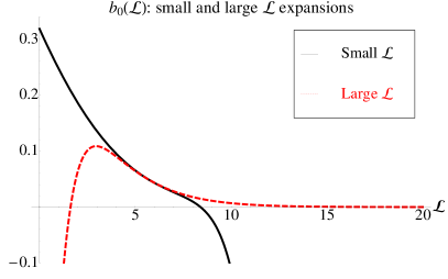
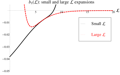
Figure 1: Large and small $\mathcal{L}$ expansions for the $b_{0}(\mathcal{L})$ and $b_{1}(\mathcal{L})$ functions. The weak coupling curve is the expansion up to $\mathcal{O}(\mathcal{L}^{12})$.

For the next function $b_{p\geq 2}(\mathcal{L})$ we could not find a closed expression and $\mathcal{L}$ dependence away from $\mathcal{L}=0$ would seem unavailable. Nevertheless, a numerical analysis shows that, in terms of $q(\mathcal{L})$, the functions

$$\widetilde{b}_{p}(q)=\frac{\mathbb{E}(q)^{2p+1}}{1-q}\,b_{p}(q),$$ (58)

appears to be rather smooth for all $0\leq q\leq 1$. This remark suggests to re-define the following functions

$$b_{p}^{[N,M]}(q)=\frac{1-q}{\mathbb{E}(q)^{2p+1}}\,{\rm Pade}[N,M,\widetilde{b}_{p}(q)],$$ (59)

where ${\rm Pade}[N,M,\widetilde{b}_{p}(q)]$ is the $[N,M]$ Padé rational approximation of $\widetilde{b}_{p}(q)$ around $q=0$. In $b_{p}^{[N,M]}(q)$, $q$ is finally substituted by the exact solution of the second equation in (2). Figure (2) shows the analysis of $b_{2}$ and $b_{3}$ which turns out to be quite robust with respect to the degrees of the Padé approximants . Thus, this method provides a simple way to obtain the complete numerical profile of all the functions $b_{p}(\mathcal{L})$.

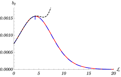
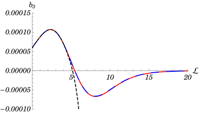
Figure 2: Padé resummation of the functions $b_{2,3}(\mathcal{L})$ as described in the main text. The dashed black line is the weak coupling expansion. The solid red line is obtained with $[N,M]=[5,4]$. The dashed blue line with $[N,M]=[6,5]$ and is numerically coincident with the previous one.

5.2 Turning on the sphere angle

The case of a non zero $\theta$ angle is discussed in Gromov:2013qga . Again the large coupling expansion of the Bremsstrahlung function can be arranged in the form:

$$\frac{1}{\theta\cot\theta}B_{L} = \frac{g}{\sqrt{\pi^{2}-\theta^{2}}}-\frac{6L+3}{8\left(\pi^{2}-\theta^{2}\right)}+\frac{3\left(\pi^{2}\left(6L^{2}+6L+1\right)-2\theta^{2}L(L+1)\right)}{128\pi^{2}g\left(\pi^{2}-\theta^{2}\right)^{3/2}}+$$ (60)

$$\frac{f_{1}}{512\pi^{4}g^{2}\left(\pi^{2}-\theta^{2}\right)^{2}}-\frac{f_{2}}{32768g^{3}\left(\pi^{6}\left(\pi^{2}-\theta^{2}\right)^{5/2}\right)}+O\left(\frac{1}{g}\right)^{4}$$

where $f_{1,2}$ are given by:

$$f_{1} = -3\theta^{4}L\left(2L^{2}+3L+1\right)+6\pi^{2}\theta^{2}L\left(2L^{2}+3L+1\right)+\pi^{4}\left(10L^{3}+15L^{2}+11L+3\right)$$

$$f_{2} = 18\theta^{6}L\left(5L^{3}+10L^{2}+7L+2\right)-18\pi^{2}\theta^{4}L\left(5L^{3}+10L^{2}+11L+6\right)-$$ (61)

$$6\pi^{4}\theta^{2}L\left(55L^{3}+110L^{2}+47L-8\right)+9\pi^{6}\left(10L^{4}+20L^{3}-22L^{2}-32L-7\right).$$

It is straightforward to check that even in this more general case all the involved polynomials satisfy (51) order by order in the small $\theta$ expansion. We can therefore apply the same argument as in the $\theta=0$ case, and derive constraints like (1).

6 Conclusions

The main results of this short paper is the $\mathbb{Z}_{2}$ symmetry (10) and its consequence (1) relating the functions $b_{2n+1}(\mathcal{L})$ to the even ones. Qualitatively, this is similar to what is found in the study of reciprocity invariance of various twist operators in $\mathcal{N}=4$ SYM. There, the anomalous dimension is a function of the operator spin $\gamma=\gamma(S)$. Under a non-linear change of variable, one introduces a related function whose large $S$ expansion involves only integer inverse powers of $S(S+1)$ at any order in the coupling constant. This means that roughly half of the terms in the $1/S$ expansion can be expressed by the other half. The relations (1) are claimed to be valid in the gauge theory and it would be very interesting to prove them by matrix model techniques as discussed in Gromov:2012eu in the case of the classical term. In principle, the discrete symmetry could also be investigated in the ${\bf P}\mu$-system Gromov:2013pga with the hope of being able to generalize it. Of course, the important open question is whether the functions $b_{p}(\mathcal{L})$ do indeed reproduce the various higher-loop semiclassical string computations. The formal equivalence of the expansion (7) with a semiclassical loop expansion in the string theory is intriguing, but only some terms could match the correspondence, beyond $b_{1}(0)$ that indeed passes the check. The simplicity of (1) holding in the gauge theory is remarkable and somewhat unexpected. An extension of the calculation in Drukker:2011za could reveal whether it remains true in the dual string theory too.

References

- (1) L. Lipatov, High-energy asymptotics of multicolor QCD and exactly solvable lattice models, hep-th/9311037.
- (2) L. Faddeev and G. Korchemsky, High-energy QCD as a completely integrable model, Phys.Lett. B342 (1995) 311–322, [hep-th/9404173].
- (3) J. Minahan and K. Zarembo, The Bethe ansatz for N=4 superYang-Mills, JHEP 0303 (2003) 013, [hep-th/0212208].
- (4) N. Beisert, C. Ahn, L. F. Alday, Z. Bajnok, J. M. Drummond, et. al., Review of AdS/CFT Integrability: An Overview, Lett.Math.Phys. 99 (2012) 3–32, [arXiv:1012.3982].
- (5) N. Beisert, B. Eden, and M. Staudacher, Transcendentality and Crossing, J.Stat.Mech. 0701 (2007) P01021, [hep-th/0610251].
- (6) N. Gromov, V. Kazakov, and P. Vieira, Exact Spectrum of Anomalous Dimensions of Planar N=4 Supersymmetric Yang-Mills Theory, Phys.Rev.Lett. 103 (2009) 131601, [arXiv:0901.3753].
- (7) D. Bombardelli, D. Fioravanti, and R. Tateo, Thermodynamic Bethe Ansatz for planar AdS/CFT: A Proposal, J.Phys.A A42 (2009) 375401, [arXiv:0902.3930].
- (8) N. Gromov, V. Kazakov, A. Kozak, and P. Vieira, Exact Spectrum of Anomalous Dimensions of Planar N = 4 Supersymmetric Yang-Mills Theory: TBA and excited states, Lett.Math.Phys. 91 (2010) 265–287, [arXiv:0902.4458].
- (9) G. Arutyunov and S. Frolov, Thermodynamic Bethe Ansatz for the Mirror Model, JHEP 0905 (2009) 068, [arXiv:0903.0141].
- (10) N. Gromov, V. Kazakov, and P. Vieira, Exact Spectrum of Planar Supersymmetric Yang-Mills Theory: Konishi Dimension at Any Coupling, Phys.Rev.Lett. 104 (2010) 211601, [arXiv:0906.4240].
- (11) A. Cavaglia, D. Fioravanti, and R. Tateo, Extended Y-system for the correspondence, Nucl.Phys. B843 (2011) 302–343, [arXiv:1005.3016].
- (12) N. Gromov, V. Kazakov, S. Leurent, and D. Volin, Solving the AdS/CFT Y-system, JHEP 1207 (2012) 023, [arXiv:1110.0562].
- (13) D. Correa, J. Maldacena, and A. Sever, The quark anti-quark potential and the cusp anomalous dimension from a TBA equation, JHEP 1208 (2012) 134, [arXiv:1203.1913].
- (14) N. Drukker, Integrable Wilson loops, arXiv:1203.1617.
- (15) A. M. Polyakov, Gauge Fields as Rings of Glue, Nucl.Phys. B164 (1980) 171–188.
- (16) G. Korchemsky and A. Radyushkin, loop space formalism and renormalization group for the infrared asymptotics of QCD, Phys.Lett. B171 (1986) 459–467.
- (17) G. Korchemsky, Asymptotics of the Altarelli-Parisi-Lipatov Evolution Kernels of Parton Distributions, Mod.Phys.Lett. A4 (1989) 1257–1276.
- (18) N. Drukker, D. J. Gross, and H. Ooguri, Wilson loops and minimal surfaces, Phys.Rev. D60 (1999) 125006, [hep-th/9904191].
- (19) K. Zarembo, Supersymmetric Wilson loops, Nucl.Phys. B643 (2002) 157–171, [hep-th/0205160].
- (20) D. Correa, J. Henn, J. Maldacena, and A. Sever, An exact formula for the radiation of a moving quark in N=4 super Yang Mills, JHEP 1206 (2012) 048, [arXiv:1202.4455].
- (21) B. Fiol, B. Garolera, and A. Lewkowycz, Exact results for static and radiative fields of a quark in N=4 super Yang-Mills, JHEP 1205 (2012) 093, [arXiv:1202.5292].
- (22) A. Bassetto, L. Griguolo, F. Pucci, and D. Seminara, Supersymmetric Wilson loops at two loops, JHEP 0806 (2008) 083, [arXiv:0804.3973].
- (23) A. Bassetto, L. Griguolo, F. Pucci, D. Seminara, S. Thambyahpillai, et. al., Correlators of supersymmetric Wilson loops at weak and strong coupling, JHEP 1003 (2010) 038, [arXiv:0912.5440].
- (24) A. Bassetto, L. Griguolo, F. Pucci, D. Seminara, S. Thambyahpillai, et. al., Correlators of supersymmetric Wilson-loops, protected operators and matrix models in N=4 SYM, JHEP 0908 (2009) 061, [arXiv:0905.1943].
- (25) J. Erickson, G. Semenoff, and K. Zarembo, Wilson loops in N=4 supersymmetric Yang-Mills theory, Nucl.Phys. B582 (2000) 155–175, [hep-th/0003055].
- (26) N. Drukker and D. J. Gross, An Exact prediction of N=4 SUSYM theory for string theory, J.Math.Phys. 42 (2001) 2896–2914, [hep-th/0010274].
- (27) N. Drukker, 1/4 BPS circular loops, unstable world-sheet instantons and the matrix model, JHEP 0609 (2006) 004, [hep-th/0605151].
- (28) N. Drukker, S. Giombi, R. Ricci, and D. Trancanelli, On the D3-brane description of some 1/4 BPS Wilson loops, JHEP 0704 (2007) 008, [hep-th/0612168].
- (29) N. Drukker, S. Giombi, R. Ricci, and D. Trancanelli, More supersymmetric Wilson loops, Phys.Rev. D76 (2007) 107703, [arXiv:0704.2237].
- (30) N. Drukker, S. Giombi, R. Ricci, and D. Trancanelli, Wilson loops: From four-dimensional SYM to two-dimensional YM, Phys.Rev. D77 (2008) 047901, [arXiv:0707.2699].
- (31) S. Giombi, V. Pestun, and R. Ricci, Notes on supersymmetric Wilson loops on a two-sphere, JHEP 1007 (2010) 088, [arXiv:0905.0665].
- (32) S. Giombi and V. Pestun, Correlators of local operators and 1/8 BPS Wilson loops on S**2 from 2d YM and matrix models, JHEP 1010 (2010) 033, [arXiv:0906.1572].
- (33) V. Pestun, Localization of gauge theory on a four-sphere and supersymmetric Wilson loops, Commun.Math.Phys. 313 (2012) 71–129, [arXiv:0712.2824].
- (34) V. Pestun, Localization of the four-dimensional N=4 SYM to a two-sphere and 1/8 BPS Wilson loops, JHEP 1212 (2012) 067, [arXiv:0906.0638].
- (35) N. Drukker and V. Forini, Generalized quark-antiquark potential at weak and strong coupling, JHEP 1106 (2011) 131, [arXiv:1105.5144].
- (36) N. Gromov and A. Sever, Analytic Solution of Bremsstrahlung TBA, JHEP 1211 (2012) 075, [arXiv:1207.5489].
- (37) N. Gromov, F. Levkovich-Maslyuk, and G. Sizov, Analytic Solution of Bremsstrahlung TBA II: Turning on the Sphere Angle, arXiv:1305.1944.
- (38) N. Gromov, V. Kazakov, S. Leurent, and D. Volin, Quantum spectral curve for , arXiv:1305.1939.
- (39) M. Beccaria, S. Giombi, G. Macorini, R. Roiban, and A. Tseytlin, ’Short’ spinning strings and structure of quantum spectrum, Phys.Rev. D86 (2012) 066006, [arXiv:1203.5710].
- (40) M. Beccaria and A. A. Tseytlin, More about ’short’ spinning quantum strings, JHEP 1207 (2012) 089, [arXiv:1205.3656].
- (41) B. Basso, An exact slope for AdS/CFT, arXiv:1109.3154.
- (42) B. Basso, Scaling dimensions at small spin in N=4 SYM theory, arXiv:1205.0054.
- (43) N. Gromov, On the Derivation of the Exact Slope Function, JHEP 1302 (2013) 055, [arXiv:1205.0018].
- (44) B. Basso and G. Korchemsky, Anomalous dimensions of high-spin operators beyond the leading order, Nucl.Phys. B775 (2007) 1–30, [hep-th/0612247].
- (45) M. Beccaria, V. Forini, and G. Macorini, Generalized Gribov-Lipatov Reciprocity and AdS/CFT, Adv.High Energy Phys. 2010 (2010) 753248, [arXiv:1002.2363].
- (46) M. Pawellek, Semiclassical Strings in AdS and Automorphic Functions, Phys.Rev.Lett. 106 (2011) 241601, [arXiv:1103.2819].