Lattice points counting via Einstein metrics

Abstract

We obtain a growth estimate for the number of lattice points inside any $\mathbb{Q}$-Gorenstein cone. Our proof uses the result of Futaki-Ono-Wang on Sasaki-Einstein metric for the toric Sasakian manifold associated to the cone, a Yau’s inequality, and the Kawasaki-Riemann-Roch formula for orbifolds.

1. Introduction

The Ehrhart polynomial $p_{P}:\mathbb{Z}\rightarrow\mathbb{Z}$ associated to a lattice polytope $P$ inside an $n$-dimensional latticed vector space $\mathbb{Z}^{n}\subset\mathbb{R}^{n}$ is given by

$$p_{P}(k)=\#(kP\cap\mathbb{Z}^{n})=\sum_{i=0}^{n}a_{i}k^{i}.$$

Lots of work has been done to get estimates of the polynomial, using either combinatorial or geometric methods (see for example [4]). In this paper, we are interested in obtaining a lower estimate of $p_{P}(k)$ for large $k$ using toric geometry and Einstein metrics.

When the polytope is Delzánt, the Ehrhart polynomial has an expression via toric geometry, by associating to $P$ a toric manifold $X_{P}$ and using the Riemann-Roch formula. It is well known that the leading coefficient $a_{n}$ is $Vol(P)$ and $a_{n-1}$ is determined by $Vol(P)$ if $P$ is reflexive. A lower estimate is obtained by considering $a_{n-2}$, which is an integral of the second Chern class of $X_{P}$, besides terms involving volume. When the polytope is balanced (i.e. the center of mass agrees with the origin), we can obtain an estimate

$$a_{n-2}\geq\frac{(3n+2)(n-1)n}{24(n+1)}Vol(P),$$

using the existence of the Kähler-Einstein metric (see [13] and [11]) and a Yau’s inequality (see appendix 4.1).

In this paper, we want to generalize this result to reflexive polytopes which may not be balanced. Given any polytope $P$, we can form its cone $C^{\lor}(P)=cone(P\times\{1\})\subset\mathbb{R}^{n}\times\mathbb{R}$ and let $\xi=(\vec{0},1)$. We count the number of lattice points up to level $k$ defined by $\xi$, that is, $n_{\xi}(k)=\#\{x\in C^{\lor}(P)\cap\mathbb{Z}^{n+1}|(x,\xi)\leq k\}$. The two counting functions are related by

$$n_{\xi}(k)=\sum_{i=0}^{k}p_{P}(i).$$

We will reformulate the counting problem by considering $n_{\xi}(k)$.

From now on, instead of using the standard lattice $\mathbb{Z}^{n}\times\mathbb{Z}$, we let $N$ be any rank $n+1$ lattice and $M$ be its dual. Let $C^{\lor}\subset M_{\mathbb{R}}$ be a cone. We can choose an affine hyperplane $H_{\xi}=\{x\in M_{\mathbb{R}}|(x,\xi)=1\}$ by picking a dual vector $\xi\in N_{\mathbb{R}}$. The hyperplane is moved toward infinity by changing $\xi$ to $\xi/k$ and letting $k\rightarrow\infty$. We consider the function

$$\begin{array}[]{rl}n_{\xi}(k)&=\#\{x\in C^{\lor}\cap M|(x,\xi)\leq k\}\\ \\ &=b_{n+1}k^{n+1}+b_{n}k^{n}+b_{n-1}k^{n-1}+\mathcal{O}(k^{n-2})\end{array}$$

which counts the number of lattice points inside the cone $C^{\lor}$ below the affine hyperplane $H_{\xi/k}$ (see §2, Figure 1). Similar to the polytope case, the first two coefficients, $b_{n+1}$ and $b_{n}$, are related to the volume of a certain polytope $\Delta_{\xi}$ determined by the $\xi$. Therefore, we focus on the first non-trivial coefficient $b_{n-1}$.

The advantage of this formulation is that we have the freedom to rotate the hyperplane by changing $\xi$. If the cone is $\mathbb{Q}$-Gorenstein (see Definition 2.1), we always have a balancing direction $\xi_{c}$ (see appendix 4.3), which satisfies

$$n_{\xi}(k)\geq n_{\xi_{c}}(k)\;\;for\;\;k\gg 0,$$

for any other normalized vector $\xi$ in the interior of the cone $C$. $\xi_{c}$ will play the role of a balancing direction for the cone $C^{\lor}$. For $\xi$ close enough to $\xi_{c}$, the coefficient $b_{n-1}$ of $n_{\xi}(k)$ will have a lower estimate.

In the case that $\xi_{c}$ is a rational vector and the polytope $\{x\in C^{\lor}|(x,\xi_{c})=1\}$ is Delzánt, our result gives

$$\begin{array}[]{rl}\frac{n_{\xi}(k)}{Vol_{n+1}(\Delta_{\xi})}\geq&k^{n+1}+\frac{(n+1)(n+2)}{2}k^{n}+\frac{n(n+1)(n+2)(3n+5)}{24}k^{n-1}+\mathcal{O}(k^{n-2}).\end{array}$$

In general, we have the following main theorem:

Main Theorem 1.

Given an $(n+1)$-dimensional $\mathbb{Q}$-Gorenstein cone $C^{\lor}\subset M_{\mathbb{R}}^{n+1}$, with its canonical Reeb vector $\xi_{c}\in C\subset N_{\mathbb{R}}$, if $\xi_{c}$ is rational, let $\xi\in N$ be a primitive vector parallel to it; otherwise, choose $\xi$ having its direction close enough to $\xi_{c}$. Then

$$\begin{array}[]{rl}b_{n+1}=&\displaystyle Vol_{n+1}(\Delta_{\xi})\\ \\ b_{n}=&\displaystyle\frac{1+q}{2}(n+1)Vol_{n+1}(\Delta_{\xi})\\ \\ b_{n-1}\geq&\displaystyle c_{q,n}Vol_{n+1}(\Delta_{\xi})\\ \\ &\displaystyle+\sum_{\rho\in C(1)}c_{\rho,n}Vol_{n}(H_{\rho})\par\par\end{array}$$

Here $\Delta_{\xi}=\{(\xi,y)\leq 1\}\subset M_{\mathbb{R}}$ is the polytope cut out by $\xi$ and $H_{\rho}=\{(\xi,y)\leq 1\}\;\cap\;\rho^{\perp}\cap C^{\lor}\subset\Delta_{\xi}$ is the corresponding facet associated to each ray $\rho\in C(1)$. $Vol_{n}$ refers to the $n$-dimensional volume of subspaces in $M_{\mathbb{R}}$.

Remark 1.

$q$ is defined in Definition 2.2. The constants $c_{q,n}$ and $c_{\rho,n}$ are given in §3 Theorem 2.

Remark 2.

The sum $\sum_{\rho\in C(1)}c_{\rho,n}Vol_{n}(H_{\rho})$ in the expansion, with $Vol_{n}(H_{\rho})$ being the volume of various facets, comes from the orbifold structures of related toric spaces.

Remark 3.

The above result can be considered purely as a problem concerning the cone $C^{\lor}$: When the direction is close enough to the canonical one minimizing the volume, we can have an estimate of the first nontrivial term in terms of the volume.

Remark 4.

In [5], Chan and the first author have studied a family of Yau’s inequalities on Fano toric manifolds and their implications in the lattice points counting problem.

We give the proof of the theorem in §2, omitting the computations that arise from the presence of orbifold singularities. The orbifold computations will be handled in §3.

2. Proof of theorem

Before giving the proof of our main theorem, we give a proof of the statement $a_{n-2}\geq\frac{(3n+2)(n-1)n}{24(n+1)}Vol(P)$ for the balanced reflexive Delzánt polytope $P$ mentioned in the introduction. Recall (see e.g. [6]) that $P$ determines a Fano toric manifold $X=X_{P}$ and $p_{P}(k)=dim_{\mathbb{C}}\Gamma(X,(K_{X}^{-1})^{\otimes k})=\chi(X,(K_{X}^{-1})^{\otimes k})$. Using the Riemann-Roch formula, we have

$$\begin{array}[]{rl}p_{P}(k)=&\int_{X}ch((K_{X}^{-1})^{\otimes k})Td(X)\\ =&(\int_{X}c_{1}^{n})\frac{k^{n}}{n!}+(\frac{1}{2}\int_{X}c_{1}^{n})\frac{k^{n-1}}{(n-1)!}+\frac{1}{12}[\int_{X}c_{1}^{n}+\int_{X}c_{1}^{n-2}c_{2}]\frac{k^{n-2}}{(n-2)!}\\ &+\mathcal{O}(k^{n-3}),\end{array}$$

where $c_{i}=c_{i}(X)$ is the $i$th Chern class of $X$. Since $P$ is balanced, $X$ has a Kähler-Einstein metric by the result of Wang-Zhu in [11]. Then we can use the Yau’s inequality,

$$\int_{X}c_{2}c_{1}^{n-2}\geq\frac{n}{2n+2}\int_{X}c_{1}^{n}$$

(see appendix 4.1), and

$$\int_{X}c_{1}^{n}=n!Vol(P)$$

to get estimate

$$a_{n-2}\geq\frac{(3n+2)(n-1)n}{24(n+1)}Vol(P).$$

Remark 5.

The Yau’s inequality and its consequences for algebraic geometry was studied by S.-T. Yau in [12], as a consequence of the existence of Kähler-Einstein metrics. The existence of such metrics was proved for the negative first Chern class case independently by T. Aubin in [3] and S.-T. Yau in [13]. The zero first Chern class case was proven by S.-T. Yau in [13].

The proof given below is in a similar flavour. We have to construct some spaces and a line bundle that count the number of lattice points. Extra difficulties arise from the orbifold structure.

As mentioned in the introduction, we consider the counting problem for a cone $C^{\lor}$. Let $C^{\lor}\subset M_{\mathbb{R}}$ be a cone; we choose an affine hyperplane $H_{\xi}=\{x\in M_{\mathbb{R}}|(x,\xi)=1\}$ by choosing a $\xi\in C\subset N_{\mathbb{R}}$ such that it cuts the cone cleanly. Move the hyperplane toward infinity by changing $\xi$ to $\xi/k$ and count the number of lattice points bounded below the hyperplane. We want to study the effect of turning the hyperplane to a different angle.

In order to make this comparison, we need to have a good parameter space of the hyperplanes with respect to the cone. This is possible if we have a $\mathbb{Q}$-Gorenstein cone.

Let $C^{\lor}\subset M_{\mathbb{R}}$ be a top dimensional rational cone, $C$ be its dual, $int(C)$ be the interior of $C$, and $C(1)$ be the set of rays in $C$ inward normal to facets in $C^{\lor}$. For each $\rho\in C(1)$, we let $v_{\rho}$ be the primitive vector in $\rho$.

Definition 2.1.

$C^{\lor}$ is said to be a $\mathbb{Q}$-Gorenstein cone if it satisfies the following two conditions.

i:

(smoothness) For each face $F\subset C^{\lor}$, the subset of $C(1)$ normal to $F$ can be extended to the $\mathbb{Z}$-basis of $N$.

ii:

($\mathbb{Q}$-Gorenstein) There exists $\lambda\in M$ and some $l\in\mathbb{Z}_{>0}$ such that $(\lambda,v_{\rho})=-l$ holds for all $\rho\in C(1)$.

Definition 2.2.

Fixing a primitive vector $\xi\in int(C)\cap M$, let $\Delta_{\xi}=\{x\in C^{\lor}|(x,\xi)\leq 1\}$ and define the lattice points counting function as

$$n_{\xi}(k)=\#(k\Delta_{\xi}\cap M).$$

For every chosen $\xi$, a ratio $q$ is defined by the equality $(\lambda,\xi)=-ql$.

The above notations and definitions are summarized in the following figure.

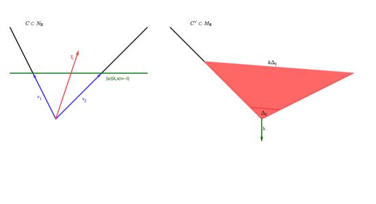
Figure 1.

$n_{\xi}(k)$ is the counting function we are interested in; we associate a non-compact toric manifold $Y_{C}$ with a $\mathbb{C}^{*}$-action to each chosen $\xi$ and relate the counting function to some geometric invariants of $Y_{C}$. We can define $\mathcal{W}$ as $Y_{C}/\mathbb{C}^{*}$, and compactify $Y_{C}\rightarrow\mathcal{W}$ as a $\mathbb{P}^{1}$ bundle $\pi:\mathcal{X}\rightarrow\mathcal{W}$. It turns out that

$$n_{\xi}(k)=\chi(\mathcal{X},\mathcal{L}^{\otimes k})$$

for some toric line bundle $\mathcal{L}$ on $\mathcal{X}$.

Remark 6.

$Y_{C}$ is related to Sasakian geometry. A quick review is given in the appendix.

For example, if $C=cone(e_{1},\dots,e_{n+1})\subset\mathbb{R}^{n+1}$ is the standard cone and $\xi$ is chosen to be $e_{1}+\dots+e_{n+1}$, then we have $Y_{C}=\mathbb{C}^{n+1}-\{0\}$, $\mathcal{W}=\mathbb{P}^{n}$, and $\mathcal{X}=\mathbb{P}_{\mathcal{W}}(\mathcal{O}(-1)\oplus\mathcal{O})$. $\mathcal{L}$ is the relative $\mathcal{O}(1)$ bundle for the map $\mathcal{X}\rightarrow\mathcal{W}.$

When $\mathcal{X}$, $\mathcal{W}$ are smooth, we have

$$\chi(\mathcal{X},\mathcal{L}^{\otimes k})=\int_{\mathcal{X}}ch(\mathcal{L}^{\otimes k})Td(\mathcal{X})$$

and we get an expression of $b_{i}$’s in terms of integrals of Chern classes on $\mathcal{W}$. In particular, $b_{n-1}$ is expressed as a combination of $Vol(\Delta_{\xi})$ and

$$\int_{\mathcal{W}}c_{2}(\mathcal{W})c_{1}(\mathcal{W})^{n-2}.$$

Furthermore, if we are lucky enough that $\xi$ is parallel to $\xi_{c}$, the above term will have a lower estimate in terms of $Vol(\Delta_{\xi})$. We indeed have a Kähler structure on $Y_{C}$ that is transversal Kähler-Einstein (appendix 4.2). In that case, this Kähler structure will induce a Kähler-Einstein structure on $\mathcal{W}$. So we can use the Yau’s inequality (appendix 4.1) to estimate it in terms of $Vol(\Delta_{\xi})$.

In general, $\xi_{c}$ may not even be rational. However, transversal Chern classes are defined and the inequality still holds. In that case, we know the transversal Yau’s inequality is strict from Lemma 2.2. For a primitive vector $\xi$ such that its direction is close enough to $\xi_{c}$, we still have our lower estimate by continuity.

Remark 7.

$\mathcal{X}$ and $\mathcal{W}$ are orbifolds in most cases.

Let us begin by giving some notations and definitions concerning the spaces mentioned above. We define a Kähler manifold $Y_{C}$ as follows: There is a map

$$\mathbb{Z}^{C(1)}\rightarrow N$$

given by the assignment

$$e_{\rho}\mapsto v_{\rho}.$$

Tensoring with $\mathbb{C}$ and taking the quotient gives rise to a group homomorphism

$$(\mathbb{C}^{*})^{C(1)}\rightarrow T_{N}^{\mathbb{C}},$$

and let $\kappa_{C}$ be the kernel. Then $Y_{C}$ is given by the G.I.T. quotient of $\mathbb{C}^{C(1)}-\{0\}$ by $\kappa_{C}$ via the natural action of $(\mathbb{C}^{*})^{C(1)}$ (see e.g. [1]).

A similar construction using the symplectic quotient gives a symplectic structure on $Y_{C}$. In general, any $\xi\in N_{\mathbb{R}}$ gives a vector field $\xi^{\#}$ on $Y_{C}$ by the real torus action. We also denote $\xi^{1,0}=\sqrt{-1}\xi^{\#}-J\xi^{\#}$ to be the corresponding holomorphic vector field. If $\xi$ is primitive, we have a $\mathbb{C}^{*}$-action on $Y_{C}$ given by the holomorphic vector field.

We define $\mathcal{W}=Y_{C}/\mathbb{C}^{*}$. Hence $Y_{C}$ can be viewed as a $\mathbb{C}^{*}$-bundle over $\mathcal{W}$. Using the standard action of $\mathbb{C}^{*}$ on $\mathbb{C}$, we can associate a line bundle $L_{\mathcal{W}}$ over $\mathcal{W}$. We let $\mathcal{X}=\mathbb{P}_{\mathcal{W}}(L_{\mathcal{W}}\oplus\mathcal{O})$ be the $\mathbb{P}^{1}$-bundle over $\mathcal{W}$. There is a relative $\mathcal{O}(1)$ bundle on $\mathcal{X}$, denoted by $\mathcal{L}$, associating to the natural projection map $\pi:\mathcal{X}\rightarrow\mathcal{W}$.

From the symplectic perspective, the space $Y_{C}$ is related to another compact odd dimensional space. If we let $r:Y_{C}\rightarrow\mathbb{R}$ be a smooth function such that $\frac{1}{2}r^{2}$ is the moment map of the induced $\mathbb{S}^{1}$-action, then $S:=\{r=1\}\subset Y_{C}$ is a principal $\mathbb{S}^{1}$-bundle over $\mathcal{W}$. $\mathcal{W}$ can be viewed as the symplectic quotient of $Y_{C}$ via the $\mathbb{S}^{1}$-action. This gives $\mathcal{W}$ a structure of Kähler orbifold.

$(S,\xi^{\#}|_{S})$ is indeed a Sasakian manifold and $(Y_{C},\xi^{\#},\omega,J)$ can be viewed as its (Kähler) cone manifold. The relationship between $(S,\xi^{\#}|_{S})$ and $(Y_{C},\xi^{\#},\omega,J)$ is a one to one correspondence. Furthermore, $(S,\xi^{\#}|_{S})$ is still defined even when $\xi$ is an irrational vector. The transversal Yau’s inequality still holds when $(S,\xi^{\#}|_{S})$ admits a transversal Kähler-Einstein metric. For details, we refer readers to [2] and [7].

From the toric perspective, in case $\xi$ is primitive, we can complete the cone $C\subset N_{\mathbb{R}}$ to a complete fan $\Sigma$ by adding $\xi$ and $-\xi$ to it. We can also define a quotient lattice $N^{\prime}=N/\mathbb{Z}\xi$ and $p:N_{\mathbb{R}}\rightarrow N_{\mathbb{R}}^{\prime}$. The image of $C$ together with its faces form a fan $\Sigma^{\prime}\subset N_{\mathbb{R}}^{\prime}$. Then we have two complete fans $\Sigma$ and $\Sigma^{\prime}$, having $|C(1)|+2$ and $|C(1)|$ rays respectively. The spaces $\mathcal{X}$ and $\mathcal{W}$ are the toric orbifolds associated to the fans $\Sigma$ and $\Sigma^{\prime}$ respectively, using the G.I.T. quotient construction (see [1]). The line bundle $\mathcal{L}$ is identified with the divisor bundle of $D_{-\xi}$.

Using the toric perspective, we have (see e.g. [6])

$$n_{\xi}(k)=dimH^{0}(\mathcal{X},\mathcal{L}^{\otimes k}).$$

In order to get

$$n_{\xi}(k)=\chi(\mathcal{X},\mathcal{L}^{\otimes k}),$$

we use the convexity of the supporting function corresponding to the line bundle $\mathcal{L}$ and the Demazure vanishing theorem [6].

Using the Kawasaki-Riemann-Roch formula in [9], we get the expansion

$$\begin{array}[]{rl}n_{\xi}(k)=&\int_{\mathcal{X}}ch(\mathcal{L}^{\otimes k})Td(\mathcal{X})+R_{orb}\\ \\ =&b_{n+1}k^{n+1}+b_{n}k^{n}+b_{n-1}k^{n-1}+\cdots.\\ \end{array}$$

Here $R_{orb}$ is the contribution from orbifold singular strata (starting from codimension 2). Presence of $R_{orb}$ results in periodicity of $b_{i}$’s in $k$ (for $i\leq n-1$); more explicitly, $b_{i}(k)$’s are composition of rational functions with functions of the form $e^{\frac{2\pi\sqrt{-1}ck}{N}}$. The contribution of $\int_{\mathcal{X}}ch(\mathcal{L}^{\otimes k})Td(\mathcal{X})$ to the coefficient $b_{n-1}$ only involves integrals of products of $c_{1}(\mathcal{W})$, $c_{1}(L_{\mathcal{W}})$, and $c_{2}(\mathcal{W})$.

First, there is an equality relating $c_{1}(\mathcal{W})$ and $c_{1}(L_{\mathcal{W}})$. Let $\xi^{1,0}$ be the holomorphic vector field on $Y_{C}$ associated to $\xi$, and let $L=\mathbb{C}\xi^{1,0}$ be the trivial line bundle over $Y_{C}$ with a Hermitian metric $\frac{1}{2}r^{2}$. Its quotient by $\mathbb{C}^{*}$ gives a Hermitian metric on $L_{\mathcal{W}}\rightarrow\mathcal{W}$ with $c_{1}(L_{\mathcal{W}}^{*})=\frac{1}{2\pi}[d\eta]$ on $\mathcal{W}$, where $\eta=d^{c}log(r)$. Here $\eta$ is the contact $1$-form of the Sasakian manifold $S$, and $d\eta$ descends to $\mathcal{W}$ (see e.g. [7]). $c_{1}(\mathcal{W})$ is also related to the class $[d\eta]$, and there is a equality

$$c_{1}(\mathcal{W})=\frac{q}{2\pi}[d\eta]=qc_{1}(L_{\mathcal{W}}^{*}),$$

where $q$ is the ratio defined in Definition 2.2.

The integral involving only the first Chern class is given in [10] by

$$\int_{\mathcal{W}}c_{1}(L_{\mathcal{W}}^{*})^{n}=(\frac{1}{2\pi})^{n+1}\int_{S}(d\eta)^{n}\wedge\eta=(n+1)!Vol(\Delta_{\xi}).$$

Second, there is a term

(1) $$\int_{\mathcal{W}}c_{2}(\mathcal{W})c_{1}(\mathcal{W})^{n-2}=\int_{S}c_{2}^{B}(S)c_{1}^{B}(S)^{n-2}\eta$$

in the expression of $b_{n-1}$. Here $c_{k}^{B}(S)$’s are basic Chern classes of $S$ defined in [7].

A key observation is that this term can be controlled if $\xi$ is suitably chosen: for our cone $C^{\lor}$, there is a canonical direction $\xi_{c}$ associated to it. (It is the unique minimizer of the volume function $F(\xi)=Vol(\{y\in C^{\lor}|(\xi,y)\leq 1\})$ restricting to $I=\{x\in int(C)|(x,\lambda)=-(n+1)l\}$.) For a general $\xi$ (may not be rational), $Y_{C}$ and $S$ are still defined and we can discuss the transversal Kähler geometry of $S$, even though the quotient $\mathcal{W}$ may not exist. Those $\xi$’s parallel to $\xi_{c}$ are exactly those with $S$ having a transversal Kähler-Einstein metric. In that case, we can obtain a lower bound of (1) by the following transversal Yau’s inequality.

Lemma 2.1 (Transversal Yau’s inequality).

Let $(S,g,J)$ be a Sasakian manifold of dimension $2n+1$ such that its transversal Ricci form satisfies

$$Ric^{T}=\tau(\frac{1}{2}d\eta)$$

for some $\tau\in\mathbb{R}$. Then

(2) $$\int_{S}[c_{2}^{B}(S)-\frac{n}{2(n+1)}(c_{1}^{B}(S))^{2}]\wedge(\frac{1}{2}d\eta)^{n-2}\wedge\eta\geq 0.$$

If the equality sign holds, then the Einstein metric has constant transversal holomorphic bisectional curvature.

As basic Chern classes depend only on the Reeb vector field $\xi^{\#}$ (or equivalently, the transversal complex structure) and not on the metric, the inequality holds whenever the Reeb vector field is given by $\xi_{c}$. It can be argued that it also holds for those $\xi$’s parallel to $\xi_{c}$. For details, readers may consult the appendix.

In the case that $\xi_{c}$ is not a rational vector, the following uniformization lemma (Lemma 2.2) tells us that we must have a strict inequality for those $\xi$’s parallel to $\xi_{c}$. Hence, for primitive $\xi$ having its direction close enough to $\xi_{c}$, we still have the same estimate.

The remainder of this section is devoted to prove Lemma 2.2. It is a statement about toric Sasakian geometry. Readers may skip the proof and progress to the next section, where we will deal with the orbifold’s contribution $R_{orb}$.

As mentioned in the appendix, given a $\mathbb{Q}$-Gorenstein cone $C^{\lor}$, we can associate to it a unique toric Sasaki-Einstein manifold $(S,g,J_{c})$ with the Reeb vector field given by $\xi_{c}$. For this space, the Yau’s inequality holds and there is a uniformization result:

Lemma 2.2.

If equality holds in (6) for the space $(S,g,J_{c})$, then $|C^{\lor}(1)|=n+1$ and $\xi_{c}$ is a rational vector.

Proof.

Step 1:

Since $C(S)=:Y$ is Ricci flat, we have a pointwise Yau’s inequality for $Y$:

$$c_{2}(Y)\wedge\omega^{n}\geq 0.$$

From the fact that $S$ has constant transversal holomorphic bisectional curvature, we have that

$$[c_{2}^{B}-\frac{n}{2(n+1)}(c_{1}^{B})^{2}]\wedge(\frac{1}{2}d\eta)^{n-2}\wedge\eta=0.$$

A second fundamental form computation implies $c_{2}(Y)\wedge\omega^{n}=0$. This further says $Y$ is flat and $S$ has positive constant sectional curvature.

Step 2:

Let $\tilde{S}$ be the universal cover of $S$ and $\tilde{Y}=C(\tilde{S})$, which is a finite covering of degree $N=|\pi_{1}(Y)|=|\pi_{1}(S)|$ as $S$ is Ricci positive. We lift the Sasakian structure to $\tilde{S}$ and hence the Kähler structure to $\tilde{Y}$. We let $p:\tilde{Y}\rightarrow Y$ be the covering map.

The torus action can be lifted to $\tilde{Y}$ (may be non-effective), and we have

$$\begin{array}[]{ccc}\mathbb{T}^{n+1}&\curvearrowright&\tilde{Y}\\ \phi\downarrow&&\downarrow\\ \mathbb{T}^{n+1}&\curvearrowright&Y,\end{array}$$

where $\phi$ is multiplication by $N$. We define $\tilde{\xi}_{c}\in\tilde{\mathfrak{t}}$ by letting $\phi_{*}(\tilde{\xi}_{c})=\xi_{c}$.

Step 3:

We may assume $Y$ is simply connected with constant holomorphic bisectional curvature by considering $\tilde{Y}$ instead. $S$, as a Riemannian manifold, is identified with the $2n+1$ dimensional sphere $\mathbb{S}^{2n+1}$. To identify the Sasakian structure, it suffices to identify the Killing vector field $K_{c}$ with $K_{std}$, generated by $\xi_{c}$ and $\xi_{std}$ respectively. Fixing a point $p_{0}\in S$, we can choose isometry between $S$ and $\mathbb{S}^{2n+1}$, which identify $(T_{p_{0}}S,K_{c}(p_{0}),\nabla K_{c}(p_{0}))$ with $(T_{1}\mathbb{S}^{2n+1},K_{std}(1),\nabla K_{std}(1))$, for some point $1\in\mathbb{S}^{2n+1}$. This identifies $K_{c}$ with $K_{std}$.

Step 4:

We have a possibly non-standard action $\mathbb{T}^{n+1}\curvearrowright\mathbb{S}^{2n+1}$. The flow line of $K_{c}$ closes up, this shows the rationality of $\xi_{c}$. Taking the quotient, we have $\mathbb{T}^{n}\curvearrowright(\mathbb{C}\mathbb{P}^{n},\omega_{std})$ being a toric Kähler manifold. Hence conjugation by automorphism of $(\mathbb{C}\mathbb{P}^{n},\omega_{std})$ gives the standard action. In particular, the moment map image is a cone with $n+1$ rays.

∎

3. Riemann-Roch for orbifolds

This section is devoted to the Riemann-Roch computation for orbifolds.

For each face $\tau\subset C$, we define

$$\tau^{1}=cone(\tau\cup\{\xi\}),\tau^{-1}=cone(\tau\cup\{-\xi\}).$$

Here $cone(F):=\{\sum_{i}a_{i}v_{i}|v_{i}\in F,a_{i}\geq 0\}$ is the cone generated by the vectors in $F$, where $F$ is a subset of a vector space. We let $\Sigma$ be the fan consisting of all $\tau$, $\tau^{1}$, $\tau^{-1}$ for all faces $\tau\subset C$. $\Sigma$ is the normal fan for the polytope $\{y\in C^{\lor}|r_{1}\leq(\xi,y)\leq r_{2}\}$ for any $r_{2}>r_{1}>0$.

As in the previous section, we have an orbifold $\mathcal{X}$, together with an orbi-line bundle $\mathcal{L}$, which compute the function $n_{\xi}(k)$:

(3) $$n_{\xi}(k)=\chi(\mathcal{X},\mathcal{L}^{\otimes k})=\int_{\mathcal{X}}ch(\mathcal{L}^{\otimes k})Td(\mathcal{X})+R_{orb}.$$

The formula for $R_{orb}$ is given in [8]. We will concentrate on the contribution of $R_{orb}$ to the coefficient $b_{n-1}$. For that purpose, we consider the codimension two singular stratum of $\mathcal{X}$ (since there is no singular stratum of codimension one).

The space $\mathcal{X}$ is a quotient of affine space $\mathbb{C}^{\Sigma(1)}$ ($\Sigma(1)$ stands for the set of all rays in the fan $\Sigma$) by some subgroup $\kappa_{\Sigma}$ of $(\mathbb{C}^{*})^{\Sigma(1)}$ via the quotient construction mentioned in [1]. Each ray in the fan corresponds to a coordinate of the affine space $\mathbb{C}^{\Sigma(1)}$ before taking the quotient. Hence vanishing of some of the coordinate functions defines a closed sub-orbifold (may be non-effective) of the quotient. For example, codimension one sub-orbifolds that correspond to rays in $\Sigma(1)$ are the toric divisors.

Codimension two closed toric sub-orbifolds are defined by two rays. For each $\rho\in C(1)$ and $\alpha$ ($\alpha=\pm 1$), we have a closed sub-orbifold $F^{\alpha}_{\rho}$ given by vanishing of the coordinate functions corresponding to the rays $\rho$ and $\alpha\xi$. These give all the singular strata necessary for the computation of the coefficient $b_{n-1}$.

To obtain a coordinate chart, we can choose an orbifold chart by taking any maximal cone $\tau\supset\rho$. By the smoothness assumption of the cone $C^{\lor}$, we can take a $\mu\in N$ together with the primitive vectors of the rays $\{v_{\rho^{\prime}}|\rho^{\prime}\in\tau(1)\}$ to be a $\mathbb{Z}$-basis of $N$ and write $\xi$ as $\xi=\sum c_{\rho^{\prime}}v_{\rho^{\prime}}+d\mu$, for some $c_{\rho^{\prime}},d\in\mathbb{Z}$. The cone $\tau^{\alpha}$ gives an orbifold chart $\mathbb{Z}_{d}\curvearrowright\mathbb{C}^{\tau(1)}\times\mathbb{C}$ of $\mathcal{X}$. $\mathbb{C}^{\tau(1)}\times\mathbb{C}\hookrightarrow\mathbb{C}^{\Sigma(1)}$ (the last coordinate corresponds to $\alpha\xi$) is a subset given by letting the coordinate functions corresponding to the rays other than $\{\alpha\xi\}\cup\tau(1)$ be $1$. The group $\mathbb{Z}_{d}$ is the subgroup of $\kappa_{\Sigma}$ which preserve the subset $\mathbb{C}^{\tau(1)}\times\mathbb{C}$. Then $\mathbb{C}^{\tau(1)}\times\mathbb{C}$ cover a dense open subset of $\mathcal{X}$. A local chart of $F^{\alpha}_{\rho}$ is given by vanishing of coordinate functions that correspond to $\rho$ and $\alpha\xi$.

If we let $\hat{d}=d/[g.c.d.(\{c_{\rho^{\prime}}\}_{\rho^{\prime}\neq\rho},d)]$ and $\Gamma_{\rho}^{\alpha}=\mathbb{Z}_{\hat{d}}\leq\mathbb{Z}_{d}$, then $\Gamma_{\rho}^{\alpha}$ acts trivially on $F^{\alpha}_{\rho}$. Let $\theta$ be the induced action of $\Gamma_{\rho}^{\alpha}$ on $\mathcal{L}|_{F_{\rho}^{\alpha}}$ ($\eta\in\Gamma_{\rho}^{\alpha}$ acts by multiplication by $\theta(\eta)$). These are the combinatorial data we needed for our computations.

According to the Kawasaki-Riemann-Roch formula in [8], we have $R_{orb}=\sum_{\rho\in C(1)}\sum_{\alpha}KRR(\rho,\alpha,\mathcal{L}^{k})+\mathcal{O}(k^{n-2}),$ where

$$\begin{array}[]{ll}&KRR(\rho,\alpha,\mathcal{L}^{\otimes k})\\ =&\displaystyle\sum_{\eta\in\Gamma_{\rho}^{\alpha}-\{0\}}\frac{\theta(\eta)^{k}}{(1-\eta^{-c_{\rho}})(1-\eta^{\alpha})}\int_{F_{\rho}^{\alpha}}\frac{c_{1}(\mathcal{L})^{n-1}}{(n-1)!}k^{n-1}+\mathcal{O}(k^{n-2}).\\ \end{array}$$

Recall that $q\in\mathbb{Q}$ is the ratio such that $(\xi,\lambda)=-ql$ ($\lambda$ as in definition (2.1)). For $n\geq 2$, we have

$$\begin{array}[]{rl}b_{n+1}=&\displaystyle\frac{1}{(n+1)!}\int_{\mathcal{W}}c_{1}(L_{\mathcal{W}}^{*})^{n}\\ \\ =&\displaystyle Vol_{M_{\mathbb{R}}}(\Delta_{\xi})\\ \\ b_{n}=&\displaystyle\frac{1}{2n!}\int_{\mathcal{W}}\{c_{1}(L_{\mathcal{W}}^{*})^{n}+c_{1}(L_{\mathcal{W}}^{*})^{n-1}c_{1}(\mathcal{W})\}\\ \\ =&\displaystyle\frac{1+q}{2}(n+1)Vol_{M_{\mathbb{R}}}(\Delta_{\xi})\\ \\ b_{n-1}=&\displaystyle\frac{(q^{2}+3q+1)}{12(n-1)!}\int_{\mathcal{W}}c_{1}(L_{\mathcal{W}}^{*})^{n}+\frac{1}{12(n-1)!}\int_{\mathcal{W}}c_{2}(\mathcal{W})c_{1}(L_{\mathcal{W}}^{*})^{n-2}\\ \\ &\displaystyle+\frac{1}{(n-1)!}\sum_{\rho,\alpha}\sum_{\eta\in\Gamma_{\rho}^{\alpha}-\{0\}}\frac{\chi(\eta)^{k}}{(1-\eta^{-c_{\rho}})(1-\eta^{\alpha})}\int_{F_{\rho}}c_{1}(L_{\mathcal{W}}^{*})^{n-1}\\ \\ =&\displaystyle\frac{(q^{2}+3q+1)}{12n(n+1)}Vol_{M_{\mathbb{R}}}(\Delta_{\xi})+\frac{1}{12(n-1)!}\int_{\mathcal{W}}c_{2}(\mathcal{W})c_{1}(L_{\mathcal{W}}^{*})^{n-2}\\ \\ &\displaystyle+\sum_{\rho\in C(1)}\frac{n}{|v_{\rho}|}\sum_{\eta\in\Gamma_{\rho}^{\alpha}-\{0\}}\frac{1-\eta^{k+1}}{(1-\eta^{-c_{\rho}})(1-\eta)}Vol_{n}(H_{\rho})\par\end{array}$$

Remark 8.

1. The equality

   $$\int_{F_{\rho}}c_{1}(L_{\mathcal{W}}^{*})^{n-1}=\frac{n!}{|v_{\rho}|}Vol_{n}(H_{\rho})$$

   is similar to that in the previous section.

2. For the case $n=1$, the formula reads

   $$\begin{array}[]{ll}\chi(\mathcal{X},\mathcal{L}^{\otimes k})\par=&\displaystyle(k^{2}+(1+q)k+q)Vol(\Delta_{\xi})\\ \\ &\displaystyle+\sum_{\rho=\{\rho_{1},\rho_{2}\}}\frac{1}{|v_{\rho}|}[\sum_{\eta\in\Gamma_{\rho}^{\alpha}-\{0\}}\frac{1-\eta^{k+1}}{(1-\eta^{-c_{\rho}})(1-\eta)}]Vol_{1}(H_{\rho})\end{array}$$

We give a $2$-dimensional example to illustrate the contribution from orbifold singularities.

Example 1.

Letting $N_{\mathbb{R}}=\mathbb{R}^{2}$, $C=cone(e_{1},-e_{1}+3e_{2})$, and $\xi=(1,1)\in\mathbb{R}^{2}$, we have $\lambda=(-3,-2)\in(\mathbb{R}^{2})^{*}$ and $q=\frac{5}{3}$. This gives $\Delta_{\xi}=cone\{(0,0),(0,1),(\frac{3}{4},\frac{1}{4})\}$, $Vol(\Delta_{\xi})=\frac{3}{8}$, $H_{e_{1}}=cone\{(0,0),(0,1)\}$, and $H_{-e_{1}+3e_{2}}=cone\{(0,0),(\frac{3}{4},\frac{1}{4})\}$ .

In this case, the lattice points counting function is

$$\eta_{\xi}(k)=\frac{1}{16}\{6k^{2}+16k+2(\sqrt{-1})^{k}[1+(-1)^{k}]+(-1)^{k}+11\}.$$

Combining with the above sections, we have our main theorem:

Main Theorem 2.

Given an $(n+1)$-dimensional $\mathbb{Q}$-Gorenstein cone $C^{\lor}\subset M_{\mathbb{R}}$, with its canonical Reeb vector $\xi_{c}\in C\subset N_{\mathbb{R}}$, if $\xi_{c}$ is rational, let $\xi\in N$ be the primitive vector parallel to $\xi_{c}$; otherwise, choose $\xi$ having its direction close enough to $\xi_{c}$. If we write

$$n_{\xi}(k)=b_{n+1}k^{n+1}+b_{n}k^{n}+b_{n-1}k^{n-1}+\mathcal{O}(k^{n-2}),$$

then we have

$$\begin{array}[]{rl}b_{n+1}=&\displaystyle Vol_{n+1}(\Delta_{\xi})\\ \\ b_{n}=&\displaystyle\frac{1+q}{2}(n+1)Vol_{n+1}(\Delta_{\xi})\\ \\ b_{n-1}\geq&\displaystyle\frac{n}{24}[q^{2}(3n+2)+2(3q+1)(n+1)]Vol_{n+1}(\Delta_{\xi})\\ \\ &\displaystyle+\sum_{\rho\in C(1)}\frac{n}{|v_{\rho}|}[\sum_{\eta\in\Gamma_{\rho}^{\alpha}-\{0\}}\frac{1-\eta^{k+1}}{(1-\eta^{-c_{\rho}})(1-\eta)}]Vol_{n}(H_{\rho})\par\par\end{array}$$

4. Appendix: Sasakian Geometry

4.1. Basic results and notations from Sasakian geometry

We recall some definitions in Sasakian geometry, following [7] and [10].

Definition 4.1.

A Sasakian manifold is a Riemannian manifold $(S,g)$ of real dimension $2n+1$, together with a choice of $\mathbb{R}$-invariant complex structure $J$ on its cone manifold $(C(S),g^{C(S)}):=(S\times\mathbb{R}_{+},dr^{2}+r^{2}g)$, such that it is Kähler.

Given a Sasakian manifold, we let $V=r\frac{\partial}{\partial r}$ be the Euler vector field and $K=JV$ be the Reeb vector field. There is an equivalent definition of Sasakian manifold from the symplectic aspect given in [2], which works better with toric geometry. We will freely interchange between the two definitions.

We follow the notations of transversal Kähler geometry of a Sasakian manifold introduced in [7].

Definition 4.2.

A Sasakian manifold $(S,g,J)$ is said to be transversal Kähler-Einstein if there is a real constant $\tau$ such that

(4) $$Ric^{T}=\tau(\frac{1}{2}d\eta)$$

where $\eta$ is the contact $1$-form on $S$.

Remark 9.

A Sasakian manifold is transversal Kähler-Einstein (with constant $\tau=2n+2$) if and only if its cone manifold $C(S)$ is Ricci flat.

To obtain a Yau’s inequality for transversal Kähler-Einstein manifolds, we recall

Theorem 4.1 (Yau’s inequality for Kähler-Einstein manifolds).

Let $(M,\omega,J,g)$ be a connected Kähler-Einstein manifold of complex dimension $n$. Then

(5) $$[c_{2}(\nabla^{l.c.})-\frac{n}{2(n+1)}c_{1}(\nabla^{l.c.})^{2}]\wedge\omega^{n-2}=\delta\omega^{n}$$

for some positive function $\delta$. $\delta\equiv 0$ if and only if $M$ has constant holomorphic bisectional curvature, where $\nabla^{l.c.}$ is the Levi-Civita connection on $M$ and $c_{i}(\nabla^{l.c.})$ is the corresponding $i$-th Chern form.

We can have the following lemma, generalizing the above to the transversal Kähler-Einstein case.

Lemma 4.1 (Transversal Yau’s inequality for Sasaki-Einstein manifolds).

Let $(S,g,J)$ be a Sasakian manifold of real dimension $2n+1$, which satisfies

$$Ric^{T}=\tau(\frac{1}{2}d\eta)$$

for some $\tau$. Then

(6) $$\int_{S}[c_{2}^{B}(S)-\frac{n}{2(n+1)}(c_{1}^{B}(S))^{2}]\wedge(\frac{1}{2}d\eta)^{n-2}\wedge\eta\geq 0,$$

where $c_{i}^{B}(S)$’s are the basic Chern classes of $S$ defined in [7]. If equality holds, then the Einstein metric has constant transversal holomorphic bisectional curvature.

Remark 10.

The above integral is independent of basic deformations of Sasakian structures described in [7].

The existence of such a metric in the case $\tau>0$ is what we are interested in. First, we normalized the constant $\tau$ by $D$-homothetic transformation to get a new Kähler metric $g^{\prime}$ with Einstein constant $2n+2$.

Given a Sasakian manifold $(S,g,J)$ and $\alpha\in\mathbb{R}_{>0}$, define $K^{\prime}=\frac{1}{\alpha}K$ and $g^{\prime}=\alpha g+\alpha(\alpha-1)\eta\otimes\eta$. The complex structure on $C(S)$, $J^{\prime}$, is given by

$$\begin{array}[]{lll}J^{\prime}(V)&=&K^{\prime}\\ J^{\prime}(Y)&=&J(Y)\;\;\;for\;\;Y\in\Gamma(T_{S})^{K^{\perp}}\\ \end{array}$$

Then we have the new Kähler form $\omega^{\prime}=\alpha\omega$ and the transversal Kähler form $\frac{1}{2}d\eta^{\prime}=\alpha(\frac{1}{2}d\eta)$.

Notice that $g^{\prime}$ has constant transversal holomorphic bisectional curvature if and only if $g$ does (with different constants).

The existence of transversal Kähler-Einstein structures is proven in the toric case by Futaki-Ono-Wang in [7].

4.2. Toric Sasakian geometry and existence of transversal Einstein metrics

For notations of toric Sasakian geometry, we refer readers to [2].

Theorem 4.2 (Futaki-Ono-Wang [7]).

For a toric Sasakian manifold with $C^{\lor}$ being its moment cone, if $C^{\lor}$ is a $\mathbb{Q}$-Gorenstein cone, then there exists a unique $J_{c}$, which is a torus invariant complex structure, such that the corresponding cone manifold is Ricci flat (or equivalently, the corresponding Sasakian manifold is transversal Kähler-Einstein).

The Reeb vector of such a Ricci flat metric is characterized by a volume minimization. Given a $\mathbb{Q}$-Gorenstein cone $C^{\lor}$, we let $F:int(C)\rightarrow\mathbb{R}$ defined by $F(\xi)=Vol_{M_{\mathbb{R}}}(\{y\in C^{\lor}|(\xi,y)\leq 1\})$, and $I=\{x\in C|(x,\lambda)=-(n+1)l\}$. Then there are the following two theorems:

Theorem 4.3 (Martelli-Sparks-Yau [10]).

$F|_{I}$ is strictly convex with a unique minimum point $\xi_{c}$.

Theorem 4.4 (Futaki-Ono-Wang [7]).

The Sasaki complex structure $J_{c}$, which admits transversal Kähler-Einstein Sasakian metric, has its Reeb vector $K_{c}$ equal to the vector field generated by $\xi_{c}$ via the torus action.

For a toric $(2n+1)$-dimensional Sasakian manifold $(S,g,J)$, by taking a $D$-homothetic transformation with constant $\alpha$, we have the new moment map and Reeb vector given by $\mu^{\prime}=\alpha\mu$ and $K^{\prime}=\frac{1}{\alpha}K$, respectively.

Hence for each $\xi\in C^{o}$ parallel to $\xi_{c}$, there is a unique $J$ having its Reeb vector field generated by $\xi$, which is transversal Kähler-Einstein.

As a consequence, for any such $J$, we have

$$\int_{S}[c_{2}^{B}-\frac{n}{2(n+1)}(c_{1}^{B})^{2}]\wedge(\frac{1}{2}d\eta)^{n-2}\wedge\eta\geq 0$$

and equality holds if and only if $J$ has constant transversal holomorphic bisectional curvature.

5. Acknowledgements

The authors thank Akito Futaki for useful discussions. The work described in this paper was substantially supported by a grant from the Research Grants Council of the Hong Kong Special Administrative Region, China (Project No. CUHK403709).

References

- [1] M. Abreu, Kähler metrics on toric orbifolds, J. Differential Geometry 58 (2001), 151–187., MR1895351, Zbl 1035.53055.
- [2] by same author, Kähler-Sasaki geometry of toric symplectic cones in action-angle coordinates, Port. Math. 67, no. 2 (2010), 121–153, MR2662864, Zbl 1193.53109.
- [3] T. Aubin, Equations du type de Monge Amp re sur les variétés kähleriennes compactes, C.R. Acad. Sci. Paris 283 (1976), 119–121., MR0433520, Zbl 0333.53040.
- [4] M. Beck and S. Robins, Computing the Continuous Discretely, Integer-point enumeration in polyhedra, Springer-Verlag, 2007, MR2271992, Zbl 1147.52300.
- [5] K. W. Chan and N. C. Leung, Miyaoka-Yau-type inequalities for Kähler-Einstein manifolds, Comm. Anal. Geom. 15 (2007), 359–379., MR2344327, Zbl 1129.14054.
- [6] D. Cox, J. Little, and H. Schenck, Toric Variety, Department of Mathematics, Amherst College, Amherst, 2010, MR2810322, Zbl 1223.14001.
- [7] A. Futaki, H. Ono, and G. Wang, Transverse Kähler geometry of Sasaki manifolds and toric Sasaki-Einstein manifolds, J. Differential Geometry 83, no. 3 (2009), 585–636., MR2581358, Zbl 1188.53042.
- [8] V. Guillemin, Riemann-Roch for toric orbifolds, J. Differential Geometry 45 (1997), 53–73., MR1443331, Zbl 0932.37039.
- [9] T. Kawasaki, The Riemann-Roch theorem for complex V-manifolds, Osaka J. Math. 16 (1979), 151–159., MR0527023, Zbl 0405.32010.
- [10] D. Martelli, J. Sparks, and S.-T. Yau, The geometric dual of -maximisation for toric Sasaki-Einstein manifolds, Comm. Math. Physics 268, no. 1 (2006), 39–65., MR2249795, Zbl 1190.53041.
- [11] X-J Wang and X. H. Zhu, Kähler-Ricci solitons on toric manifolds with positive first Chern class, Advances in Math. 188 (2004), 87–103., MR2084775, Zbl 1086.53067.
- [12] S.-T. Yau, Calabi’s conjecture and some new results in algebraic geometry, Proc. Nat. Acad. Sci. USA 74 (1977), 1798–1799., MR0451180, Zbl 0355.32028.
- [13] by same author, On the Ricci curvature of a compact Kähler manifold and the complex Monge-Ampére equation I, Comm. Pure Appl. Math. 31 (1978), 339–411., MR0480350, Zbl 0369.53059.