Nature of the epidemic threshold for the susceptible-infected-susceptible dynamics in networks

Abstract

We develop an analytical approach to the susceptible-infected-susceptible (SIS) epidemic model that allows us to unravel the true origin of the absence of an epidemic threshold in heterogeneous networks. We find that a delicate balance between the number of high degree nodes in the network and the topological distance between them dictates the existence or absence of such a threshold. In particular, small-world random networks with a degree distribution decaying slower than an exponential have a vanishing epidemic threshold in the thermodynamic limit.

The accurate theoretical understanding of epidemic thresholds on complex networks is a pressing challenge in the field of network science Albert and Barabási (2002); Dorogovtsev and Mendes (2003); Newman (2010). Indeed, such a knowledge has potential practical applications in the design of optimal immunization programs Pastor-Satorras and Vespignani (2002); Cohen et al. (2003) and may shed light on the behavior of the viral spreading of rumors, fads and beliefs Goffman and Newill (1964); Leskovec et al. (2007). In this respect, a large research effort has been recently devoted to the study of the susceptible-infected-susceptible (SIS) epidemic model Anderson and May (1992), the simplest model of epidemic spreading showing an absorbing state phase transition between a healthy and an endemic phase at a critical value of the effective infective rate $\lambda$ Marro and Dickman (1999). The behavior of the SIS model is particularly relevant in the case of highly heterogeneous networks, for which a vanishing epidemic threshold in the thermodynamic limit has been pointed out Pastor-Satorras and Vespignani (2001). Recently, a scientific controversy has arisen concerning the location and the real nature of the epidemic threshold in this kind of networks Castellano and Pastor-Satorras (2010, 2012); Goltsev et al. (2012); Lee et al. (2012). In this paper, we provide strong analytical and numerical arguments showing that the threshold asymptotically vanishes in any network with a degree distribution decaying slower than exponentially, thus clarifying the physical origin of this behavior.

In the SIS model, individuals can be in one of two states, either susceptible or infected. Susceptible individuals become infected by contact with infected individuals at rate $\lambda$ times the number of infected contacts. Infected individuals, on the other hand, become spontaneously healthy again at rate $\mu$ that, without loss of generality, is set to unity. The original approach to the dynamics of the SIS model Pastor-Satorras and Vespignani (2001) was based on the so-called heterogeneous mean-field (HMF) theory Dorogovtsev et al. (2008); Barrat et al. (2008), which neglects both dynamical and topological correlations. To do so, the actual quenched structure of the network—given by its adjacency matrix $A_{ij}$ Newman (2010)—is replaced by an annealed version, in which edges are constantly rewired at a rate much faster than that of the epidemics, while preserving the degree distribution $P(k)$. According to HMF theory, the epidemic threshold of the SIS model takes the form $\lambda_{c}^{\mathrm{HMF}}=\langle{k}\rangle/\langle{k^{2}}\rangle$ Pastor-Satorras and Vespignani (2001), where $\langle{k}\rangle$ and $\langle{k^{2}}\rangle$ are the first and second moments of $P(k)$ Newman (2010). Many real networks have a heterogeneous degree distribution, often scaling as a power-law (PL), $P(k)\sim k^{-\gamma}$ Albert and Barabási (2002); Dorogovtsev and Mendes (2003); Newman (2010). This implies that the second moment diverges with the maximum degree $k_{max}$ for a degree exponent $\gamma<3$, leading to a threshold scaling $\lambda_{c}^{\mathrm{HMF}}\sim k_{max}^{\gamma-3}$, which vanishes in the thermodynamic limit. On the other hand, for $\gamma>3$, the second moment is finite and consequently so the epidemic threshold.

While HMF theory represents an exact result in the case of annealed networks Boguñá et al. (2009); Ferreira et al. (2012), its validity for real (quenched) networks is limited. Indeed, an important improvement over HMF theory is given by the quenched mean-field theory (QMF) Chakrabarti et al. (2008); Van Mieghem et al. (2009); Gomez et al. (2010) which, while still neglecting dynamical correlations, takes into account the full form of $A_{ij}$. Within this framework, the epidemic threshold is predicted to be $\lambda_{c}^{\mathrm{QMF}}=1/\Lambda_{N}$, where $\Lambda_{N}$ is the largest eigenvalue of the adjacency matrix. Given the scaling of $\Lambda_{N}$ with the maximum degree, $\Lambda_{N}\sim\max\{\sqrt{k_{max}},\langle{k^{2}}\rangle/\langle{k}\rangle\}$ Chung et al. (2003), QMF theory predicts the same result as HMF theory for $\gamma<5/2$, while for $\gamma>5/2$ it leads to $\lambda_{c}^{\mathrm{QMF}}\sim 1/\sqrt{k_{max}}$, that is, to a vanishing threshold for any value of $\gamma$ (even for $\gamma>3$) in the thermodynamic limit Castellano and Pastor-Satorras (2010). The prediction of QMF theory has been validated for $\gamma<3$ by means of large scale numerical simulations based on the quasi-stationary state method Ferreira et al. (2012). Numerical evidence for $\gamma>3$ is, however, less convincing and has led to the following two criticisms.

Goltsev et al. Goltsev et al. (2012) have considered, within the QMF framework, the effects of eigenvector localization on the steady state of the SIS model. According to their observations, in PL networks with $\gamma<5/2$, the principal eigenvector is delocalized, which implies that the density of infected nodes is finite above $\lambda_{c}^{\mathrm{QMF}}$. However, for $\gamma>5/2$, the principal eigenvector is localized, meaning that above $\lambda_{c}^{\mathrm{QMF}}$ the system is active but activity is concentrated around the hubs and their neighbors, leading to a number of infected nodes that scales sub-linearly with system size and, therefore, does not constitute a true endemic state. The endemic state should, instead, appear at a different threshold, inversely proportional to the eigenvalue of the upper delocalized state, and approximately corresponding to the HMF value Goltsev et al. (2012). Therefore, the true threshold to the endemic state would have a finite value for $\gamma>3$, at odds with the interpretation of QMF theory made in Castellano and Pastor-Satorras (2010).

This view is further pursued by Lee et al. Lee et al. (2012) by partly taking into account dynamical correlations. Their argument is as follows: Slightly above the QMF threshold, hubs in a PL network become active but their activity is restricted to their immediate neighborhood. This activity has a characteristic lifetime $\tau(k,\lambda)$ depending on the degree and the value of the spreading rate $\lambda$. When hubs are directly connected to each other (the case of a clustered network, in the nomenclature of Ref. Lee et al. (2012)), activity can be transferred between hubs if the lifetime $\tau(k,\lambda)$ is sufficiently large. In this case, above $\lambda_{c}^{\mathrm{QMF}}$ the network is able to support an endemic state, characterized by the mutual reinfection of connected hubs. In the case of unclustered networks, however, hubs are not directly connected and the reinfection mechanism does not work. Thus, the authors of Ref. Lee et al. (2012) claim that the state above $\lambda_{c}^{\mathrm{QMF}}$ is just a Griffiths phase Vojta (2006), where the density of infected nodes decays with time more slowly than exponentially (logarithmically indeed), while the actual epidemic threshold is located at a higher, finite value of $\lambda$. Within this picture a true zero epidemic threshold in the thermodynamic limit occurs only for $\gamma<3$.

While the arguments presented in Refs. Goltsev et al. (2012); Lee et al. (2012) are appealing and, apparently, leading to the conclusion that the threshold is finite in random PL networks with $\gamma>3$, here we reconsider the problem and provide analytical and numerical evidence pointing in the opposite direction, namely, a vanishing epidemic threshold for any small-world network with a degree distribution decaying slower than exponentially, in particular power-law networks with any $\gamma$. To confirm this prediction, we propose a numerical approach, based on the scaling analysis of the survival time of the infection process, which is able to provide very accurate estimates of the epidemic threshold even in the regime where the quasi-stationary state method is unreliable.

Our analytical approach is based on the consideration of dynamical correlations, as in Lee et al. (2012), but not restricted to direct neighbors. The argument of Lee et al. (2012) assumes that a zero epidemic threshold can only occur in clustered networks, when hubs are directly connected to each other and can reinfect each other within a time smaller that the characteristic healing time $\tau$. However, as already pointed out in Ref. Chatterjee and Durrett (2009), a direct connection is not a necessary condition for the possibility of hub reinfection. Instead, we should properly consider the possibility of reinfection between two vertices $i$ and $j$, separated by a topological distance $d_{ij}$, possibly larger than $1$. Indeed, the epidemic threshold predicted by the HMF theory is actually based on the local properties of the network alone, assuming that the local structure will replicate in a tree like fashion forever, preserving only the statistical properties of the network. Then, above $\lambda_{c}^{\mathrm{HMF}}$, we expect that a perturbation originated in a node will be able to propagate as a supercritical branching process forever. Below this threshold, this process is not possible. Still, as we show below, the epidemics can sustain itself, due to perturbations which propagate up to distances of order $\ln(N)$, where $N$ is the network size.

To take into account dynamical correlations over distant neighbors, we replace the original SIS dynamics by a modified description of the SIS process valid over coarse-grained time scales. On such longer temporal intervals, it is possible that a given infected node $i$ propagates the the infection to any other node $j$ in the network via a sequence of microscopic infection events of intermediate, nearest neighbors nodes. The infective rate $\lambda$ is then replaced by the effective rate $\bar{\lambda}(d_{ij},\lambda)$ at which the infected node $i$ infects any other node $j$ in the network when the process is mediated by a chain of $d_{ij}-1$ intermediate nodes. On the coarse-grained time scale also the recovery rate $\delta$ of node $i$ is replaced by an effective rate $\bar{\delta}(k_{i},\lambda)$. Overall, the evolution of the SIS dynamics over the coarse-grained time scale is then given by

$$\frac{d\rho_{i}(t)}{dt}=-\bar{\delta}(k_{i},\lambda)\rho_{i}(t)+\sum_{j\neq i}\bar{\lambda}(d_{ij},\lambda)\rho_{j}(t)[1-\rho_{i}(t)],$$ (1)

which is defined on a fully connected graph. The parameters $\bar{\delta}$ and $\bar{\lambda}$ reflect in this description the structure of the original network. On long time scales node $i$ is considered as susceptible only when the node and all of its nearest neighbors in the original graph are susceptible: hence its recovery rate is $\bar{\delta}(k_{i},\lambda)=\tau^{-1}(k_{i},\lambda)\approx e^{-a(\lambda)k_{i}}$ (see SI for numerical results and an analytical argument sup ), where $a(\lambda)$ is a smooth growing function of $\lambda$. To evaluate the effective infective rate it is convenient to assume that paths connecting nodes are independent and made of nodes of degree $2$. This leads to the expression $\bar{\lambda}(d_{ij},\lambda)\approx\lambda e^{-b(\lambda)(d_{ij}-1)}$, with $b(\lambda)=\ln(1+1/\lambda)$ (see SI for an analytical derivation and a numerical validation sup ). The assumptions made for determining $\bar{\lambda}$ are clearly not true in a real network because there are many paths connecting the same pair of nodes and intermediate nodes have, in general, degrees larger than 2. This implies that the infective rate between two nodes that we use in the coarse-grained SIS dynamics is smaller than the real one. Therefore, Eq. (1) will provide an upper bound for the true epidemic threshold of the original SIS dynamics and, thus, the absence of an epidemic threshold of the former will imply also its absence in the latter.

Eq. (1) can be applied to any network. We can, however, get deeper insights in the case of small-world random graphs, in which the the average internode topological distance takes the form Hołyst et al. (2005)

$$d_{kk^{\prime}}=1+\frac{\ln{\left(\frac{N\langle k\rangle}{kk^{\prime}}\right)}}{\ln{\kappa}}$$ (2)

where $\kappa=\langle{k^{2}}\rangle/\langle{k}\rangle-1$ is the average branching factor of the network. Using the approximation Eq. (12) allows us to coarse grain Eq. (1) for degree classes. After defining $\rho_{k}(t)\equiv\sum_{deg(i)=k}\rho_{i}(t)/NP(k)$ and plugging Eq. (12) into Eq. (1), we obtain

$$\frac{d\rho_{k}(t)}{dt}=-\bar{\delta}(k,\lambda)\rho_{k}(t)$$

$$+ \lambda N\left[\frac{k}{N\langle k\rangle}\right]^{\frac{b(\lambda)}{\ln{\kappa}}}\sum_{k^{\prime}}k^{\prime\frac{b(\lambda)}{\ln{\kappa}}}P(k^{\prime})\rho_{k^{\prime}}(t)[1-\rho_{k}(t)].$$

Notice that the use of Eq. (12) implies that the local propagation of the infection among directly connected nodes is neglected; only reinfections between distant ($\sim\ln N$) nodes are taken into account. By performing a linear stability analysis of this equation, we can see that the critical epidemic threshold of the coarse-grained SIS dynamics, $\lambda_{c}$, is the solution of the transcendental equation (see SI for a detailed derivation sup )

$$1=\lambda N\sum_{k=k_{min}}^{k_{max}}P(k)\tau(k,\lambda)\left[\frac{k^{2}}{N\langle k\rangle}\right]^{\frac{b(\lambda)}{\ln{\kappa}}}.$$ (4)

In general, the maximum degree of the network, $k_{max}$, is a growing function of $N$. If we further assume that the degree distribution decays slower than an exponential, Eq. (4) can be approximated as the integral near the upper bound $k_{max}$, i.e.

$$1=\frac{\lambda}{a(\lambda)}e^{a(\lambda)k_{max}-\frac{b(\lambda)}{\ln{\kappa}}\ln\left[\frac{N\langle k\rangle}{k_{max}^{2}}\right]-\ln\left[\frac{1}{NP(k_{max})}\right]}.$$ (5)

When $P(k)$ decays slower than an exponential, $k_{max}$ grows faster than $\ln{N}$. Therefore, as the system size grows while keeping $\lambda$ fixed, there is a point where the first term in the exponential becomes larger than the other two (negative) terms and, eventually, the right hand side of Eq. (4) becomes larger than $1$. As a consequence, the epidemic threshold of the coarse-grained SIS dynamics starts decreasing as $N$ increases, thus going to zero in the thermodynamic limit. Making the additional assumption that $a(\lambda)\approx a\lambda^{2}$ for $\lambda\ll 1$ (which is compatible with numerical simulations, see SI sup ), we conclude that the upper bound of the epidemic threshold decreases as $1/\sqrt{k_{max}}$, with additional logarithmic corrections to scaling. Interestingly, this scaling is similar to the one predicted by the QMF theory. However, in our case, the threshold marks the onset of a true endemic state where a finite fraction of all nodes of the system are active.

The case of non small-world networks can be considered along the same lines. Unfortunately, a general formula for the average topological distance as a function of nodes’ degrees is not known. Nevertheless, the absence of long range connections in non small-world networks suggests that node degree is not as determinant as in the case of small-world ones. Thus, to get some understanding, we assume an internode distance independent of the degree and scaling as a power-law with system size, i.e. $d=1+\alpha N^{\beta}$. An analysis similar to the case of small-world networks (see SI sup ) concludes that non small-world networks have a vanishing epidemic threshold only if $k_{max}$ grows faster than $N^{\beta}$. This result explains the finite epidemic threshold in the $(3,3)$-flower model Rozenfeld et al. (2007) found in Ref. Lee et al. (2012), even if the model generates a PL network with $\gamma=1+\ln{6}/\ln{2}\approx 3.58$. Indeed, this model generates a non small-world network with $\beta=\ln{3}/\ln{6}$ whereas $k_{max}\sim N^{\ln{2}/\ln{6}}$ Rozenfeld et al. (2007).

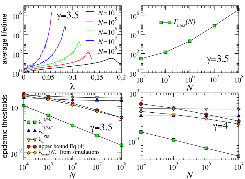
Figure 1: (color online) Top plots (single network realization): (left) Average lifetime of finite realizations for PL random graphs with $\gamma=3.5$, $k_{min}=3$ and different sizes; (right) divergence of the height of the peak in $\bar{T}(\lambda)$ as a function of the network size. Bottom plots (averages over 5 network realizations): Epidemic thresholds as measured in numerical simulations in PL networks of different sizes, $\gamma=3.5$, $k_{min}=3$ and $\gamma=4$, $k_{min}=2$. It is also shown the upper bound predicted by our theory as found from a numerical solution of Eq. (4) with $\tau(k,\lambda)$ measured in numerical simulations. For the sake of comparison, we also show the QMF, HMF, and SIR thresholds.

To check the accuracy of our theory, we propose a method to estimate the critical point of absorbing state phase transitions. The method is based on the analysis of individual realizations of the process starting with a single infected node. Each realization is characterized by its lifetime $T$ and coverage $C$, where the latter is defined as the fraction of distinct nodes ever infected during the realization. In the thermodynamic limit, realizations can be of two types: finite or endemic. Finite realizations have a finite lifetime and, therefore, a vanishing coverage in the thermodynamic limit. Endemic realizations, on the other hand, have an infinite lifetime and their coverage is equal to 1. Below the epidemic threshold, all realizations are trivially finite. Above the threshold, there is a non null probability, $P_{end}(\lambda)$, that a realization that starts at a single node becomes endemic, making $P_{end}$ a good order parameter of the phase transition. Akin to the role of the average size of finite clusters in standard percolation Stauffer and Aharony (1994), in our approach the role of susceptibility is played by the average lifetime of finite realizations $\bar{T}(\lambda)$, which diverges at $\lambda_{c}$ both from below and above.

In finite systems, the major problem is to determine when a realization is endemic or not. One possibility is to declare a realization as endemic whenever its coverage reaches 1. However, from a computational point of view, this option is too costly. We therefore take advantage of the following fact: In an infinite size system, whenever the coverage of a realization reaches a finite fraction (even small), the probability of the realization being endemic is 1. Then, in finite systems, we declare a realization as endemic whenever its coverage reaches a predefined value (in our case $C=0.5$, see SI for tests with other values sup ) and stop the realization at this point. Then, we can measure the average lifetime of finite realizations $\bar{T}(\lambda,N)$ and the position of its peak, which we take as the estimate of the epidemic threshold for finite systems. Finally, we note that the method can be applied starting from any node of the network with identical results as far as the position of the threshold is concerned. Here, to minimize the fluctuations of $\bar{T}(\lambda,N)$ close to the critical point, we start our simulations always from the node with highest degree.

Figure 1 shows the result of this program in random PL networks generated with the uncorrelated configuration model Catanzaro et al. (2005). The average lifetime $\bar{T}(\lambda,N)$ behaves as an effective susceptibility and, thus, we estimate the epidemic threshold for a finite network as the position of its peak, $\lambda_{max}(N)$. These estimates are shown in the bottom plots and compared with the upper bound given by a numerical solution of Eq. (4) and where $\tau(k,\lambda)$ is obtained from numerical simulations. As it can be clearly seen, the upper bound predicted by our theory is in very good agreement with numerical simulations, even for $\gamma=4$, a network clearly “unclustered” according to Lee et al. (2012).

Notice that, due to the approximation made in Eq. (12), our theory neglects the propagation of the epidemic mediated only by connected nodes, which is the approach taken in the HMF theory. Therefore, one should expect that the true upper bound for the real epidemic threshold is the minimum between the estimation given by Eq. (4) and $\lambda_{c}^{\mathrm{HMF}}$. From this perspective, it is surprising that the epidemic threshold measured from simulations is higher than $\lambda_{c}^{\mathrm{HMF}}$ for small system sizes. Notice, however, that the HMF theory of the SIS dynamics completely neglects dynamical correlations. These correlations account for the fact that, whenever a node is infected, there is a high probability for the node that infected it to be still infected. Therefore, the number of neighbors available to an infected node to further propagate the epidemics is, in most cases, its degree minus 1. Consequently, a better upper bound for the local propagation of the dynamics is given by the HMF theory of the SIR model, that is $\lambda_{c}^{SIR}=\langle k\rangle/\langle k(k-1)\rangle$. Bottom plots of Fig. 1 show the estimation of $\lambda_{c}^{SIR}$, which is always above the real threshold.

To sum up, the behavior of the SIS epidemic threshold in networks depends on a delicate balance between their local and global properties. Both HMF and QMF theories are constructed by considering only the local dynamics of infections among nearest neighbors, and thus fail to provide a correct description. Here we have presented a theoretical approach to epidemics in networks, built upon previously sketched concepts, that takes into account the full network structure, and that considers reinfection events among nodes not directly connected, i.e. mediated by chains of other nodes. Our theoretical analysis, while based in some (reasonable) approximations, is well backed up by means of reliable numerical evidence. The main conclusion of both approaches is that the epidemic threshold in SIS model is effectively null in the thermodynamic limit in all random small-world networks with a degree distribution decaying slower than exponentially. Beyond this remarkable result, our work highlights the subtle role that dynamical correlations might play in non-equilibrium heterogeneous systems near criticality.

I Supplementary Information

Appendix A Numerical simulations

The SIS dynamics is simulated with a continuous time dynamics as follows: During the course of the simulation, we keep track of the number of infected nodes $N_{I}(t)$ and the number of active links $E_{A}(t)$, where an active link is defined as a link emanating from an infected node (notice that links connecting two infected nodes will appear twice in this list). At each step, with probability $p_{r}=N_{I}(t)/[N_{I}(t)+\lambda E_{A}(t)]$, a randomly chosen infected node is turned susceptible whereas, with probability $1-p_{r}$, an active link is chosen at random and if one of the two nodes attached to the link is susceptible, then this node is turned infected. After this procedure, time is updated as $t\rightarrow t+1/[N_{I}(t)+\lambda E_{A}(t)]$ and the list of infected nodes and active links recomputed. An equivalent algorithm keeps a list of active links as those connecting one infected node and one susceptible. The advantage of this latter method is that infectious attempts always end up with a susceptible node being infected, which is not the case with the first method. In this work, all simulations are backed up independently with the two methods.

Appendix B Estimation of the infective rate $\bar{\lambda}(d_{ij},\lambda)$

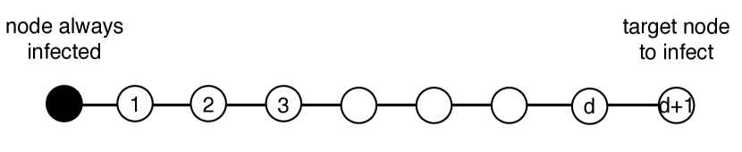
Figure 2: Scheme of the infectious events mediated by chains of nodes.

This rate is the inverse of the average time infected node $i$ takes to infect node $j$ when they are separated by a distance $d_{ij}$ in the original graph. We consider the process of transmission of the infection between the two nodes mediated by a one dimensional chain of length $d_{ij}$. Consider a one dimensional chain of $d+2$ nodes with the leftmost node always infected, as indicated in Fig. 2. Let $T(d+1)$ the average time the node at the rightmost position takes to get infected for the first time. Let $\tilde{T}(d)$ the average time between two consecutive infectious events (after the first one) of the node at distance $d$. Because we are in a chain and the source of the infection is the leftmost node, the node at distance $d+1$ can only get infected for the first time by its left neighbor. Once this node is infected, the probability that the target node gets the infection before its left neighbor recovers is simply given by

$$p=\frac{\lambda}{1+\lambda}$$ (6)

the node at distance $d+1$ can get infected right after its left node gets infected for the first time or after the second time, and so on. The probability that the node gets infected right after its left neighbor gets infected for the $n-$th time is

$$\mbox{Prob}(n)=p(1-p)^{n-1}$$ (7)

On the other hand, the average time elapsed in this case $T_{n}(d+1)$ is

$$T_{n}(d+1)=T_{n}(d)+(n-1)(1+\tilde{T}(d))+\lambda^{-1}.$$ (8)

Combining these two results, we get the equation for the average infection time, $T(d)=\sum_{n}\mbox{Prob}(n)T_{n}(d)$,

$$T(d+1)=T(d)+\frac{2}{\lambda}+\frac{1}{\lambda}\tilde{T}(d)$$ (9)

with the initial conditions $T(1)=\tilde{T}(1)=\lambda^{-1}$. In the limit of low infectious rate, that is, $\lambda\ll 1$, we can approximate $\tilde{T}(d)\approx T(d)$ and we get a closed recursive equation for $T(d)$, whose solution is

$$T(d)=\frac{1}{\lambda}\left[\left(1+2\lambda\right)\left(1+\frac{1}{\lambda}\right)^{d-1}-2\lambda\right]\approx\frac{1}{\lambda}e^{(d-1)\ln{\left(1+\frac{1}{\lambda}\right)}}$$ (10)

We then conclude that the infective rate is

$$\bar{\lambda}(d_{ij},\lambda)\approx\lambda e^{-b(\lambda)(d_{ij}-1)},\mbox{ with }b(\lambda)=\ln{\left(1+\frac{1}{\lambda}\right)}$$ (11)

In the case of small-world random graphs, the average internode topological distance depends only on the degree of the nodes as Hołyst et al. (2005)

$$d_{k,k^{\prime}}=1+\frac{\ln{\left(\frac{N\langle k\rangle}{kk^{\prime}}\right)}}{\ln{\kappa}}.$$ (12)

Inserting this expression into the effective infective rate we get

$$\lambda_{k,k^{\prime}}=\lambda\left[\frac{kk^{\prime}}{\langle{k}\rangle N}\right]^{\frac{b(\lambda)}{\ln{\kappa}}}.$$ (13)

We test numerically this relationship by keeping a single node of degree $k$ always infected and computing the time it takes to infect for the first time any other node in the network. The rate $\lambda_{k,k^{\prime}}$ is obtained by inverting the value of this time for the first infectious event, averaged over all nodes of degree $k^{\prime}$. Equation (13) predicts that plotting $\left[\lambda_{k,k^{\prime}}/\lambda\right]^{\ln{\kappa}/b(\lambda)}$ vs $k^{\prime}$ a linear behavior must be found, and this turns out to agree with the outcome of simulations in a network with $\gamma=3.5$ (see Fig. 3).

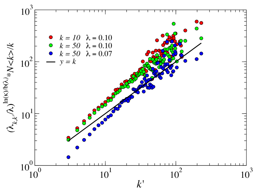
Figure 3: Plot of $\left[\lambda_{k,k^{\prime}}/\lambda\right]^{\ln{\kappa}/b(\lambda)}\cdot N\langle{k}\rangle/k$ vs $k^{\prime}$ for various values of $\lambda$ and $k$. The prediction of Eq. (13) is the straight solid line.

Appendix C Estimation of the recovery rate $\delta(k,\lambda)$

This rate can be estimated as the inverse of the survival time of an infection starting at the center of a star of degree $k$. Unfortunately, the exact solution to this problem is rather involved (see Cator and Van Mieghem (2013) for an exact treatment). Here, we present an approximation based on the discretization of the process in time units of $\mu^{-1}=1$. Consider the following cycle: initially, the center of the star –the hub– is infected whereas leaf nodes are susceptible. The probability that a leaf node is infected when the hub recovers is

$$p_{in}=\frac{\lambda}{2+\lambda}.$$ (14)

Then, by the time the hub recovers, there are $n$ infected leaf nodes with probability

$$\mbox{Prob}(n|k)=\left(\begin{array}[]{c}k\\ n\end{array}\right)p_{in}^{n}(1-p_{in})^{k-n}$$ (15)

the probability that at least one of these $n$ infected nodes infects the hub again before they recover is

$$\sum_{n=1}^{k}\mbox{Prob}(n|k)[1-(1-p_{in})^{n}]=1-(1-p_{in}^{2})^{k}.$$ (16)

The average time to complete the cycle is $2$. The probability that the outbreak goes through a sequence of $m$ complete cycles and then dies is

$$(1-p_{in})^{k}\left[1-(1-p_{in}^{2})^{k}\right]^{m};m=0,1,\cdots$$ (17)

and the time elapsed $(2m+1)$. However, an outbreak can also die in the middle of the cycle, that is, when infected leaves recover before infecting the hub again. The probability that the outbreak goes through a sequence of $m$ complete cycles and dies in the middle of the $m+1$ cycle is

$$\left[(1-p_{in}^{2})^{k}-(1-p_{in})^{k}\right]\left[1-(1-p_{in}^{2})^{k}\right]^{m};m=0,1,\cdots$$ (18)

The average elapsed time is in this case $(2m+2)$. Putting these pieces together, the effective recovery rate can be approximated as

$$\delta^{-1}(k,\lambda)=\frac{2}{(1-p_{in}^{2})^{k}}-\frac{1}{(1+p_{in})^{k}}.$$ (19)

For low infectious rates $p_{in}\ll 1$, this can be approximated as

$$\delta^{-1}(k,\lambda)\approx 2e^{-\lambda^{2}k/4}.$$ (20)

As we have mentioned at the beginning of this section, the previous calculations provide only an approximation to the true recovery rate. This is so because we have considered the process as discretized in time whereas the real process takes place at continuous time. Nevertheless, we expect that Eq. (20) captures the correct functional dependence. To check this result, we have performed simulations of the SIS model on star graphs, starting from a state with only the hub infected and computed the average time needed to reach the absorbing healthy state. Fig. 4 shows the average lifetime for fixed values of $\lambda$ as a function of the degree $k$, where the exponential trend predicted by our calculations is clearly visible.

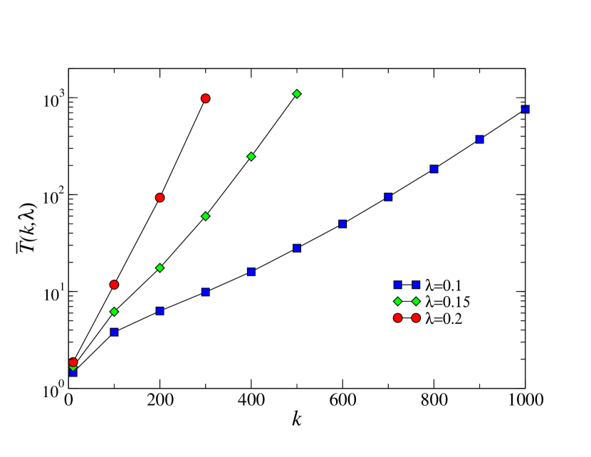
Figure 4: Average lifetime of star graphs with the hub originally infected as a function of the star degree and different values of $\lambda$.

Appendix D Derivation of Eq. (4)

Let us consider Eq. (3) in the main paper, namely

$$\frac{d\rho_{k}(t)}{dt}=-\bar{\delta}(k,\lambda)\rho_{k}(t)+\lambda N\left[\frac{k}{N\langle k\rangle}\right]^{\frac{b(\lambda)}{\ln{\kappa}}}\sum_{k^{\prime}}k^{\prime\frac{b(\lambda)}{\ln{\kappa}}}P(k^{\prime})\rho_{k^{\prime}}(t)[1-\rho_{k}(t)].$$ (21)

It is obvious that the absorbing state $\rho_{k}(t)=0$ is a fixed point of the dynamics. Therefore, we conclude that an endemic state exists whenever the solution $\rho_{k}=0$ is dynamically unstable. Following this idea, we linearize Eq. (21) around $\rho_{k}=0$, i.e.,

$$\frac{d\rho_{k}(t)}{dt}\approx-\bar{\delta}(k,\lambda)\rho_{k}(t)+\lambda N\left[\frac{k}{N\langle k\rangle}\right]^{\frac{b(\lambda)}{\ln{\kappa}}}\sum_{k^{\prime}}k^{\prime\frac{b(\lambda)}{\ln{\kappa}}}P(k^{\prime})\rho_{k^{\prime}}(t).$$ (22)

This equation can be written in matrix form as

$$\frac{d\rho_{k}(t)}{dt}\approx\sum_{k^{\prime}}\mathbb{M}_{kk^{\prime}}\rho_{k^{\prime}}(t),$$ (23)

where

$$\mathbb{M}_{kk^{\prime}}=-\bar{\delta}(k,\lambda)\delta_{kk^{\prime}}+\lambda N\left[\frac{k}{N\langle k\rangle}\right]^{\frac{b(\lambda)}{\ln{\kappa}}}k^{\prime\frac{b(\lambda)}{\ln{\kappa}}}P(k^{\prime}).$$ (24)

The stability of the absorbing state is then controlled by the maximum eigenvalue of matrix $\mathbb{M}$, that is, the maximum $\Lambda_{m}$ solution of the eigenvalue problem $\mathbb{M}\vec{u}=\Lambda\vec{u}$. In this way, $\Lambda_{m}=0$ defines the threshold between the absorbing and endemic phases. The eigenvalue problem can be rewritten as

$$\frac{\lambda N}{\Lambda+\bar{\delta}(k,\lambda)}\left[\frac{k}{N\langle k\rangle}\right]^{\frac{b(\lambda)}{\ln{\kappa}}}\sum_{k^{\prime}}k^{\prime\frac{b(\lambda)}{\ln{\kappa}}}P(k^{\prime})u_{k^{\prime}}=u_{k},$$ (25)

which gives us the explicit dependence of $u_{k}$ on $k$. Using this result, the eigenvalues satisfy the equation

$$\sum_{k}P(k)\frac{\lambda N}{\Lambda+\bar{\delta}(k,\lambda)}\left[\frac{k^{2}}{N\langle k\rangle}\right]^{\frac{b(\lambda)}{\ln{\kappa}}}=1.$$ (26)

By setting $\Lambda=0$ and recalling that $\tau(k,\lambda)=\bar{\delta}(k,\lambda)^{-1}$, we recover Eq. (4) in the main paper.

Appendix E Non small-world networks

Let us assume that the average distance is given by

$$d=1+\alpha N^{\beta}.$$ (27)

Plugging this expression in Eq. (1) in the main paper, we obtain a coarse description of the dynamics as

$$\frac{d\rho_{k}(t)}{dt}=-\bar{\delta}(k,\lambda)\rho_{k}(t)+\lambda Ne^{-\alpha N^{\beta}\frac{b(\lambda)}{\ln{\kappa}}}\sum_{k^{\prime}}P(k^{\prime})\rho_{k^{\prime}}(t)[1-\rho_{k}(t)].$$ (28)

By repeating the same analysis performed in the previous section, we conclude that the critical infection rate satisfies the equation

$$1=\lambda Ne^{-\alpha N^{\beta}\frac{b(\lambda)}{\ln{\kappa}}}\sum_{k}P(k)\tau(k,\lambda).$$ (29)

Assuming again that $P(k)$ decays slower than an exponential, this equation can be approximated as

$$1=\frac{\lambda}{a(\lambda)}e^{a(\lambda)k_{max}-\alpha N^{\beta}\frac{b(\lambda)}{\ln{\kappa}}-\ln\left[\frac{1}{NP(k_{max})}\right]}.$$ (30)

From this equation it is easy to see that for any fixed value of $\lambda$, if $k_{max}$ grows faster than $N^{\beta}$, there exists a size $N$ such that the exponent in this equation starts growing with the system size and, therefore, the right hand side in this equation will eventually grow above 1. The logical consequence is that, in this case, the epidemic threshold goes to zero as $N$ goes to infinity.

Appendix F Robustness with respect to the coverage threshold $C$

To determine whether a given realization of the SIS process is endemic, we have used the condition that the coverage is larger than a fixed threshold value $C=0.5$. To check that different assumptions do not qualitatively change the results, we performed some numerical tests. In Fig. 5, we consider the effect of changing $C$ for an Erdös-Rényi graph of average degree $\langle{k}\rangle=5$ and different sizes $N$. The numerical estimate of the threshold rapidly converges to the expected value $\lambda_{c}=1/5$ for both values of $C$ considered, while the height of the peak grows with an exponent independent of $C$.

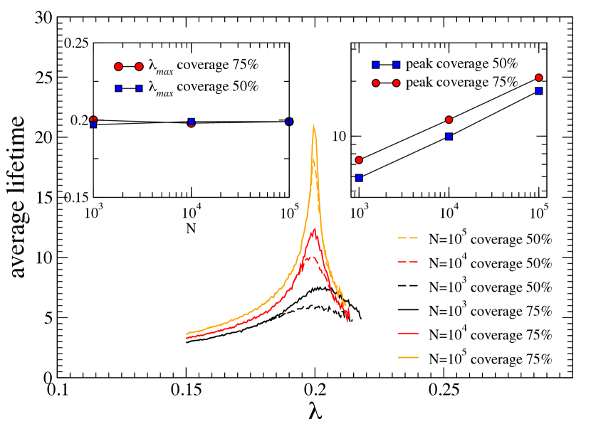
Figure 5: Main: average lifetime $\bar{T}(\lambda,N)$ for finite realizations as a function of $\lambda$ for the SIS model on an Erdös-Rényi graph of average degree $\langle{k}\rangle=5$. Left inset: position of the peak marking the estimate of the numerical threshold as a function of the system size $N$. Right inset: height of the peak as a function of $N$.

In Fig. 6, we perform the same analysis for a UCM graph with $\gamma=3.5$ and $k_{min}=3$, obtaining similar results. As the system size $N$ is increased, the estimated thresholds decrease and the peak heights increase in a perfectly analogous way.

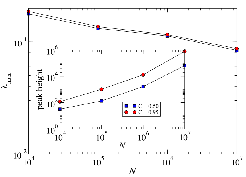
Figure 6: Main: value of the epidemic threshold $\lambda_{max}$ estimated numerically as the position of the peak of $\bar{T}(\lambda,N)$ as a function of $N$ for a UCM network with $\gamma=3.5$ and $k_{min}=3$. Inset: height of the peak of $\bar{T}(\lambda,N)$ for the same system.

Both figures confirm that the behavior of the model is robust with respect to the arbitrary choice of the coverage threshold $C$.

Appendix G Further characterization of the epidemic transition

In this section we provide some additional insight into the transition marked by the peak of the average lifetime of finite realizations $\bar{T}(\lambda,N)$. In Fig. 7, we compare the curves already plotted in the top left of Fig. 1 of the main paper with the analogous curves computed for a star graph with $k_{max}$ leaves.

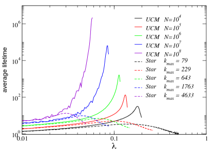
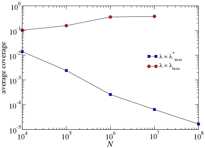
Figure 7: Left: Plot of the average lifetime of finite realizations $\bar{T}(\lambda,N)$ for UCM networks with $\gamma=3.5$ and $k_{min}=3$ and increasing values (bottom to top) of the system size $N$ (solid lines). Dashed lines are the same quantity computed for a star graph made of $k_{max}+1$ nodes, where the values of $k_{max}$ are equal to the largest degree in the UCM networks. Right: Plot of the average coverage for a UCM network with $\gamma=3.5$ and $k_{min}=3$ for two different values of $\lambda$, corresponding to the thresholds for the whole network ($\lambda_{max}$) and for the star graph centered around the largest hub ($\lambda^{*}_{max}$).

It is clear that the occurrence of the peak in the full network is not due only to the star graph centered around its hub. The latter sustains alone the activity only for small $\lambda$. The transition occurs at higher values of $\lambda$, for which the lifetime is exceedingly larger.

In Fig. 7 we plot, as a function of $N$, the value of the average coverage of the whole network at the critical value $\lambda_{max}(N)$ and at the critical value $\lambda_{max}^{*}(N)$ for the star graph centered around the hub of degree $k_{max}$. It turns clearly out that at the critical point $\lambda_{max}$ the coverage assumes a finite value in the thermodynamical limit, while it vanishes for $\lambda=\lambda_{max}^{*}$. For $\lambda=\lambda_{max}^{*}$ the hub and its neighbors are fully covered, yet the epidemics does not escape from the hub and its neighbors and it is thus localized. At the transition point $\lambda_{max}$ instead the epidemics leaves the hub and affects the whole population, leading to a truly endemic state.

References

- Albert and Barabási (2002) R. Albert and A.-L. Barabási, Rev. Mod. Phys. 74, 47 (2002).
- Dorogovtsev and Mendes (2003) S. N. Dorogovtsev and J. F. F. Mendes, Evolution of networks: From biological nets to the Internet and WWW (Oxford University Press, Oxford, 2003).
- Newman (2010) M. E. J. Newman, Networks: An introduction (Oxford University Press, Oxford, 2010).
- Pastor-Satorras and Vespignani (2002) R. Pastor-Satorras and A. Vespignani, Phys. Rev. E 65, 036104 (2002).
- Cohen et al. (2003) R. Cohen, S. Havlin, and D. ben Avraham, Phys. Rev. Lett. 91, 247901 (2003).
- Goffman and Newill (1964) W. Goffman and V. A. Newill, Nature 204, 225 (1964).
- Leskovec et al. (2007) J. Leskovec, L. A. Adamic, and B. A. Huberman, ACM Trans. Web 1, 5 (2007).
- Anderson and May (1992) R. M. Anderson and R. M. May, Infectious diseases in humans (Oxford University Press, Oxford, 1992).
- Marro and Dickman (1999) J. Marro and R. Dickman, Nonequilibrium Phase Transitions in Lattice Models (Cambridge University Press, Cambridge, 1999).
- Pastor-Satorras and Vespignani (2001) R. Pastor-Satorras and A. Vespignani, Phys. Rev. Lett. 86, 3200 (2001).
- Castellano and Pastor-Satorras (2010) C. Castellano and R. Pastor-Satorras, Phys. Rev. Lett. 105, 218701 (2010).
- Castellano and Pastor-Satorras (2012) C. Castellano and R. Pastor-Satorras, Nature Scientific Reports 2, 371 (2012).
- Goltsev et al. (2012) A. V. Goltsev, S. N. Dorogovtsev, J. G. Oliveira, and J. F. F. Mendes, Phys. Rev. Lett. 109, 128702 (2012).
- Lee et al. (2012) H. K. Lee, P.-S. Shim, and J. D. Noh, e-print arXiv:1211.2519 (2012).
- Dorogovtsev et al. (2008) S. N. Dorogovtsev, A. V. Goltsev, and J. F. F. Mendes, Rev. Mod. Phys. 80, 1275 (2008).
- Barrat et al. (2008) A. Barrat, M. Barthélemy, and A. Vespignani, Dynamical Processes on Complex Networks (Cambridge University Press, Cambridge, 2008).
- Boguñá et al. (2009) M. Boguñá, C. Castellano, and R. Pastor-Satorras, Phys. Rev. E 79, 036110 (2009).
- Ferreira et al. (2012) S. C. Ferreira, C. Castellano, and R. Pastor-Satorras, Phys. Rev. E 86, 041125 (2012).
- Chakrabarti et al. (2008) D. Chakrabarti, Y. Wang, C. Wang, J. Leskovec, and C. Faloutsos, ACM Trans. Inf. Syst. Secur. 10, 1 (2008).
- Van Mieghem et al. (2009) P. Van Mieghem, J. Omic, and R. Kooij, IEEE ACM T. Network. 17, 1 (2009).
- Gomez et al. (2010) S. Gómez, A. Arenas, J. Borge-Holthoefer, S. Meloni, and Y. Moreno, Europhysics Letters 89, 38009 (2010).
- Chung et al. (2003) F. Chung, L. Lu, and V. Vu, Proc. Natl. Acad. Sci. USA 100, 6313 (2003).
- Vojta (2006) T. Vojta, Journal of Physics A: Mathematical and General 39, R143 (2006).
- Chatterjee and Durrett (2009) S. Chatterjee and R. Durrett, Annals of Probability 37, 2332 (2009).
- (25) See Supplementary Information for additional details, numerical results, and theoretical methods.
- Hołyst et al. (2005) J. A. Hołyst, J. Sienkiewicz, A. Fronczak, P. Fronczak, and K. Suchecki, Phys. Rev. E 72, 026108 (2005).
- Rozenfeld et al. (2007) H. D. Rozenfeld, S. Havlin, and D. ben Avraham, New Journal of Physics 9, 175 (2007).
- Stauffer and Aharony (1994) D. Stauffer and A. Aharony, Introduction to Percolation Theory (Taylor & Francis, London, 1994), 2nd ed.
- Catanzaro et al. (2005) M. Catanzaro, M. Boguñá, and R. Pastor-Satorras, Phys. Rev. E 71, 027103 (2005).
- Cator and Van Mieghem (2013) E. Cator and P. Van Mieghem, Phys. Rev. E 87, 012811 (2013).