Are the ’weak measurements’ really measurements?

Abstract

’Weak measurements’ can be seen as an attempt at answering the ’Which way?’ question without destroying interference between the pathways involved. Unusual mean values obtained in such measurements represent the response of a quantum system to this ’forbidden’ question, in which the ’true’ composition of virtual pathways is hidden from the observer. Such values indicate a failure of a measurement where the uncertainty principle says it must fail, rather than provide an additional insight into physical reality.

Q. What time is it when the clock strikes 13?

A. Time to buy a new clock.

(A joke)

I Introduction

Twenty five years ago Aharonov, Albert and Vaidman published a paper entitled ”How the Result of a Measurement of a Component of the Spin of a Spin-1/ 2 Particle Can Turn Out to be 100?” W1 . The authors’ idea was further developed a large volume of work on the so-called ’weak measurements’ (see, for example, W2 -W10 ), culminating in a somewhat bizarre the BBC report BBC suggesting that ”Pioneering experiments have cast doubt on a founding idea of the branch of physics called quantum mechanics”. There seems to be room for discussion about what actually happens in a ’weak measurement’, and this is the subject of this paper. Some of the early and more recent criticisms of the original approach used in Ref. W1 can be found in Refs. C1 -C5 .
There appear to be only two possible answers to the original question posed by the authors of Ref.W1 : (I) there is a new counter-intuitive aspect to quantum measurement theory, or (II) the proposed measurement is flawed. In this paper we will follow Ref. C3 in advocating the second point of view. The argument is subtle. There is no error in the simple mathematics of the Ref. W1 . It is the interpretation of the result which is at stake. Below we will argue that a ’weak measurement’ attempts to answer the ’Which way?’ question without destroying interference between the pathways of interest. Such an attempt must be defeated by the Uncertainty Principle Feyn , Bohm and the unusual ’weak values’ are just the evidence of the defeat.

II Probabilities and ’negative probabilities’

A random variable $f$ is fully described by its probability distribution $\rho(f)$. Often it is sufficient to know only the typical value of $f$, and the range over which the values are likely to be spread. To get an estimate for the centre and the width of the range, one usually evaluates the mean value of $f$,

$${\langle}f{\rangle}=\int f\rho(f)df/\int\rho(f)df$$

and the standard mean deviation $\sigma=\sqrt{{\langle}f^{2}{\rangle}-{\langle}f{\rangle}^{2}}$.
Suppose $f$ can only take the values $1$ and $2$, and its unnormalised probability distribution is $\rho(1)=1.1$ and $\rho(2)=1$. We, therefore, have

$${\langle}f{\rangle}=[1\times\rho(1)+2\times\rho(2)]/[\rho(1)+\rho(2)]\approx 1.4761,$$ (1)

$$\sigma\approx 0.4994,$$

which reasonably well represent the centre and width of the interval $[1,2]$ containing the values of $f$.
Suppose next that, for whatever reason, the unnormalised probabilities were allowed to take negative values, e.g.

$$\rho(1)=-1.1,{\quad}\rho(2)=1.$$ (2)

Using the same formulas, we find

$${\langle}f{\rangle}=-9,{\quad}{\quad}\sigma\approx 10.49i.$$ (3)

which, clearly, no longer describe the range $[1,2]$, - $|{\langle}f{\rangle}|$ is too large, and $\sigma$ is purely imaginary. The reason for obtaining such an ’anomalous’ mean value is that the denominator in Eq.(1) is small, while the numerator is not - hence the large negative ’expectation value’ in Eq.(3).
In general, the mean and the standard mean deviation of an alternating distribution do not have to represent the region of its support. These useful properties of ${\langle}f{\rangle}$ and $\sigma$ are lost, once a distribution is allowed to change its sign.

III Complex valued distributions

To make things worse, let us assume that the unnormalised ’probabilities’ $\rho(f)$ are also allowed to take complex values,

$$\rho(f)=\rho_{1}(f)+i\rho_{2}(f),$$ (4)

while $f$ may take any value inside an interval $[a,b]$. As before, we will construct a normalised distribution $w(f)\equiv\rho(f)/\int_{a}^{b}\rho(f^{\prime})df^{\prime}$, which can now be written as a sum of its real and imaginary parts,

$$w(f)\equiv w_{1}(f)+iw_{2}(f)=\quad\quad\quad\quad\quad\quad\quad\quad\quad\quad\quad\quad\quad\quad\quad\quad$$ (5)

$$\frac{A_{1}^{2}(\rho_{1}(f)/A_{1})+A_{2}^{2}(\rho_{2}(f)/A_{2})}{A_{1}^{2}+A_{2}^{2}}+iA_{1}A_{2}\frac{\rho_{2}(f)/A_{2}-\rho_{1}(f)/A_{1}}{A_{1}^{2}+A_{2}^{2}},$$

where $\int_{a}^{b}\rho(f)df=A_{1}+iA_{2}$.
Now we may wonder whether the value of $Re{\langle}f{\rangle}=\int_{a}^{b}fw_{1}(f)df$ would give us an idea about the location of the interval $[a,b]$. From Eq.(5) we note that if both $\rho_{1}(f)$ and $\rho_{2}(f)$ do not change sign, $w_{1}(f)$ is a proper probability distribution, and its mean certainly lies within the region of its support. If, on the other hand, both $\rho_{1}(f)$ and $\rho_{2}(f)$ alternate, the mean $Re{\langle}f{\rangle}$ is allowed to lie anywhere, and is not obliged to tell us anything about the actual range of values of $f$.
So here is how a confusion might arise: suppose one needs to evaluate the average of a variable known to take values between $1$ and $2$ indirectly, i.e., without checking whether the distribution alternates, or is a proper probabilistic one. Obtaining a result of $-9$ may seem unusual, until it is realised that the employed distribution changes sign, and ’scrambles’ the information about the actual range values involved.
One remaining question is why was it necessary to employ such a tricky distribution in the first place?

IV Feynman’s Uncertainty Principle and the ’Which way?’ question

A chance to employ oscillatory complex valued distribution is offered by quantum mechanics, and for a good reason. Consider a kind of double-slit experiment in which a quantum system, initially in a state $|I{\rangle}$, may reach a given final state $|F{\rangle}$ via two pathways, the corresponding probability amplitudes being $A(1)$ and $A(2)$. There are two possibilities.
(I) The pathways interfere, and the probability to reach $|F{\rangle}$ is given by

$$P^{F\leftarrow I}=|A(1)+A(2)|^{2}.$$ (6)

(II) Interference between the pathways has been completely destroyed by bringing the system in contact with another system, or an environment. Now the probability to reach $|F{\rangle}$ is

$$P^{F\leftarrow I}=|A(1)|^{2}+|A(2)|^{2}.$$ (7)

The two cases are physically different, as are the two probabilities. In the second case the two pathways are ${\it real}$. One can make an experiment which would confirm by multiple trials that the system travels either the first or the second route with frequencies proportional to $|A(1)|^{2}$ and $|A(2)|^{2}$, respectively. In the first case the pathways remain ${\it virtual}$. Together they form a single real pathway travelled with probability $|A(1)+A(2)|^{2}$, and there is no way of saying, even statistically, which of the two virtual paths the system has actually travelled.

The above leads to a loose formulation of the Uncertainty Principle Feyn : several interfering pathways or states should be considered as a single unit. Quantum interference erases detailed information about a system. This information can only be obtained if interference is destroyed, usually at the cost of perturbing the system’s evolution, thus destroying also the very studied phenomenon, e.g., an interference pattern in Young’s double-slit experiment.

V Feynman paths and pathways

Let us go about the pathways in a slightly more formal way. By slicing the time interval into $N$ subintervals, and sending $N$ to infinity, we can write the transition amplitude for a system with a Hamiltonian $\hat{H}$ as a sum over paths traced by a variable $\hat{A}$,

$${\langle}F|\exp(-i\hat{H}t/\hbar)|I{\rangle}=lim_{N\rightarrow\infty}\sum_{k_{1},k_{2},...k_{N+1}}\times$$ (8)

$${\langle}F|a_{k_{N+1}}{\rangle}{\langle}a_{k_{N+1}}|exp(-i\hat{H}t/\hbar N)|a_{k_{N}}{\rangle}{\langle}a_{k_{N}}|...|a_{k_{2}}{\rangle}{\langle}a_{k_{2}}|exp(-i\hat{H}t/\hbar N)|a_{k_{1}}{\rangle}{\langle}a_{k_{1}}|I{\rangle}$$

$$\equiv\sum_{paths}A^{F\leftarrow I}[path]$$

where $a_{k}$ and $|a_{k}{\rangle}$ are the eigenvalues and eigenvectors of the variable of interest $\hat{A}$, $\hat{A}|a_{k}{\rangle}=a_{k}|a_{k}{\rangle}$. We also introduced Feynman paths - functions which take the values $a_{k}$ from the spectrum of $\hat{A}$ at each discrete time. In the limit $N\to\infty$ we will denote such a path by $a(t)$. The paths are virtual pathways, each contributing a probability amplitude $A^{F\leftarrow I}[path]$ defined in Eq.(8). In the chosen representation they form the most detailed complete set of histories available to the quantum system.
We may be interested not in every detail of the particle’s past, but only in the value of a certain variable, a functional defined for a Feynman path $a(t)$ as an integral

$$\mathcal{F}[path]=\int_{0}^{t}\beta(t^{\prime})a(t^{\prime})dt^{\prime},$$ (9)

where $\beta(t)$ is a known function of our choice. We can define a less detailed set of virtual pathways by grouping together those paths for which the value of $\mathcal{F}[a]$ equals some $f$. Each pathway now contributes the amplitude

$$\Phi^{F\leftarrow I}(t|f)=\sum_{paths}\delta(f-\mathcal{F}[path])A^{F\leftarrow I}[path],$$ (10)

where $\delta(z)$ is the Dirac delta. The new pathways contain the most detailed information about the variable $\mathcal{F}$, while information about other variables has been lost to interference in the sum (10).
Next we can define a coarse grained amplitude distribution for $\mathcal{F}$ by smearing $\Phi^{F\leftarrow I}(t|f)$ with a ’window’ function $G(f)$ :

$$\Psi^{F\leftarrow I}(t|f)=\int G(f-f^{\prime})\Phi^{F\leftarrow I}(t|f^{\prime})df^{\prime}.$$ (11)

With $G(f)$ chosen, for example, to be a Gaussian of a width $\Delta f$ we are unable to distinguish the values $f_{1}$ and $f_{2}$ less than $\Delta f$ apart, $|f_{1}-f_{2}|\lesssim\Delta f$, since the corresponding pathways may now interfere.
The coarse graining does, however, have a physical meaning. Consider a basis $\{F\}$ containing our final state $|F{\rangle}$, and construct a state $|\Psi^{I}(t|f){\rangle}\equiv\sum_{F}|F{\rangle}\Psi^{F\leftarrow I}(t|f)$ so that $\Psi^{F\leftarrow I}(t|f)={\langle}F|\Psi^{I}(t|f){\rangle}$. It is easy to check DS2013 that $\Psi^{I}(t|f){\rangle}$ satisfies a differential equation,

$$i\partial_{t}|\Psi^{I}(t|f){\rangle}=[\hat{H}-i\hbar\partial_{f}\beta(t)\hat{A}|\Psi^{I}(t|f){\rangle}$$ (12)

with the initial condition

$$|\Psi^{I}(t=0|f){\rangle}=G(f)|I{\rangle},$$ (13)

This can also be seen as a Schroedinger equation describing a system interacting with a von Neumann pointer vN whose position is $f$. With it we have the recipe for measuring the the quantity $\mathcal{F}[path]$: first prepare the system in the initial state $|I{\rangle}$ and the pointer in the state $\int G(f)|f{\rangle}df$. Switch on the coupling, and at a time $t$ measure the pointer position accurately. Interference between paths with different values of $\mathcal{F}[path]$ will be destroyed, since they lead do different outcomes for the pointer.

VI The accuracy and the back action

Our measurement scheme has an important parameter, the width of the window $G(f)$, $\Delta f$, which determines the extent to which we can ascertain the value of $\mathcal{F}[path]$, once the pointer has been found in $f$. This accuracy parameter also determines the perturbation a measurement exerts on the measured system. This, in turn, can be judged by how much the probability to arrive in a final state $|F{\rangle}$ with the meter on differs from that with the meter off. The former is given by

$$P^{F\leftarrow I}(t)=\int df|\Psi^{F\leftarrow I}(t|f)|^{2},$$ (14)

and, in general, is not equal to $|{\langle}F|\exp(-i\hat{H}t/\hbar)|I{\rangle}|^{2}$ since

$$\int G(f-f^{\prime})\Phi^{F\leftarrow I}(t|f^{\prime})df^{\prime}\neq G(f){\langle}F|\exp(-i\hat{H}t/\hbar)|I{\rangle}=G(f)\int\Phi^{F\leftarrow I}(t|f^{\prime})df^{\prime},$$ (15)

where the last equality is obtained by integrating Eq.(10).
The perturbation can be minimised by choosing $G(f)$ to be very broad. By construction, the value of $\mathcal{F}$ typically lies within a finite interval, say, $a\leq\mathcal{F}[path]\leq b$, outside of which $\Phi^{F\leftarrow I}(t|f^{\prime})$ vansihes. A very broad $G(f-f^{\prime})$ can, therefore be replaced by $G(f)$, making the l.h.s. of Eq.(15) proportional to ${\langle}F|\exp(-i\hat{H}t/\hbar)|\Psi_{0}{\rangle}$.
Thus, in order to study the system with the interference between the pathways intact, we must make a highly inaccurate ’weak’ measurement. This can be achieved by introducing a high degree of uncertainty in the pointer’s initial position. The following classical example may give us some encouragement.

VII Inaccurate classical measurements

Consider a classical system which can reach a final state by several different routes. Let us say, a ball can roll from a hole $I$ to a hole $F$ down the first groove with the probability $w_{1}>0$, or down the second groove, with the probability $w_{2}>0$, and so on. It is easy to imagine a (purely classical) pointer which moves one unit to the right if the ball travels the first route, or two units to the right, if the second route is travelled, and so on. The meter is imperfect: we can accurately determine its final position, while we cannot be sure that it has been set exactly at zero. Rather, its initial position is distributed around $0$ with a probability density $G(f)$ of a zero mean and a known variance. Let there be just two routes. Now the final meter readings are also uncertain, with the probability to find it in $f$ given by

$$P^{F\leftarrow I}(f)=\int G(f-f^{\prime})w(f^{\prime})df^{\prime}$$ (16)

$$w(f)\equiv w_{1}\delta(f-1)+w_{2}\delta(f-2).$$

If the meter is accurate, i.e., if $G(f)$ is very narrowly peaked around $f=0$, we will have just two possible readings, $f=1$, in approximately $w_{1}N$ out of $N$ trials, or $f=2$, in approximately $w_{2}N$ out of all cases.
Suppose next that the meter is highly inaccurate, and the width of $G$, $\Delta f$ is much larger than $1$. A simple calculation shows C3 that the first two moments of the final distribution are given by

$${\langle}f{\rangle}=\int fw(f)df,\quad\quad\quad\quad\quad\quad\quad\quad\quad\quad\quad\quad$$ (17)

$${\langle}f^{2}{\rangle}=\int f^{2}w(f)df+\int f^{2}G(f)df/\int G(f)df.$$

We have, therefore, a very broad distribution, whose mean coincides with the mean of the $w(f)$. Since the second moment of $G$ is known, by performing a large number of trials we can extract from the data also the variance $\sigma$ of $w(f)$. For instance, if the two routes are travelled with equal probabilities, $w_{1}=w_{2}=1/2$, we have

$${\langle}f{\rangle}=1.5,{\quad}\sigma=0.5.$$ (18)

From this we can correctly deduce that there are just two, and not three or four, routes available to the system, and that they are travelled with roughly equal probabilities. This simple example shows that, classically, even a highly inaccurate meter can yield limited information about the alternatives available to a stochastic system. It is just a matter of performing a large number of trials required to gather the necessary statistics. Next we will see whether this remains true in the quantum case.

VIII Inaccurate, or ’weak’, quantum measurements,

In the quantum case, employing an inaccurate meter has a practical advantage - we minimise the back action of the meter on the measured system, and may hope to learn something without destroying the interference. As discussed in Sect. VI, we can make a measurement non-invasive by giving the initial meter’s position a large quantum uncertainty (that is to say, we choose a pure meter state broad in the coordinate space). We prepare the system and the pointer in a product state (13), turn on the interaction, check the system’s final state, and sample the meter’s reading provided this final state is $|F{\rangle}$. From (12) the moments of the distribution of the meter’s readings are given by

$${\langle}f^{n}{\rangle}\equiv\int f^{n}|\Psi^{F\leftarrow I}(t|f)|^{2}df/\int|\Psi^{F\leftarrow I}(t|f)|^{2}df.$$ (19)

As the width of the initial meter’s state $\Delta f$ tends to infinity, assuming $ImG(f)=0$ we have C3

$${\langle}f{\rangle}=Re\bar{f}+O(1/\Delta f),$$ (20)

and

$${\langle}f^{2}{\rangle}=\frac{\int f^{2}G(f)^{2}df}{\int G(f)^{2}df}+C(Re\bar{f^{2}}-|\bar{f}|^{2})+|\bar{f}|^{2}+O(1/\Delta f).$$ (21)

where $C$ is a factor of order of unity, which depends only on the shape of $G(f)$ C3 . and we have introduced the notation $\bar{f^{n}}$ for the $n$-th moment of the complex valued amplitude distribution $\Phi(f)$ defined in Eq.(10),

$$\bar{f^{n}}\equiv\int f^{n}\Phi^{F\leftarrow I}(t|f)df/\int\Phi(t|f)df.$$ (22)

It is at this point that ’improper’ averages (22) evaluated with oscillatory distributions enter our calculation, originally set to evaluate ’proper’ probabilistic averages (20). Expressions similar to Eq.(20) have been obtained earlier in W1 ; W4 for a weak von Neumann measurement and in SB for the quantum traversal time. They are the quantum analogues of the classical Eqs.(17).
We see that the quantum case turned out to be different in one important aspect. Where the inaccurate classical calculation of the previous Section yielded the mean of the probability distribution, its quantum counterpart gives us the mean evaluated with the probability amplitude $\Phi^{F\leftarrow I}(t|f)$. There is no apriori reason to expect that either its real or imaginary part does not change sign. As discussed in Sects. II and III, such averages are not obliged to tell us anything about the actual range of a random variable. Thus, our attempt to answer the ’Which way?’ (’Which $f$?’) question is likely to fail, as we are not able to extract the information about the alternatives available to a quantum system. But we have been warned: the Uncertainty Principle suggests that, for as long as the pathways remain interfering alternatives, the question we ask has no meaning.

IX A double slit experiment

To give our approach a concrete example, we return to the double slit experiment. Consider a two-level system, e.g., a spin-1/2 precessing in a magnetic field. The Hamiltonian is given by

$$\hat{H}=\hbar\omega_{L}\sigma_{x}$$ (23)

where $\omega_{L}$ is the Larmor frequency, and $\sigma_{x}$ is the Pauli matrix. We assume that the spin is pre-selected in a state polarised along the $z$-axis at $t=0$, and then post-selected in the same state at $t=T$. We also wish to know the state of the spin half-way through the transition, at $t=T/2$. We follow the steps outlines in Sect. V. At any given time, and in the given representation, the spin can point up or down the $z$-axis. We label these two sates $|1{\rangle}$ and $|2{\rangle}$, respectively. Feynman paths are, therefore, irregular curves shown in Fig. 1.

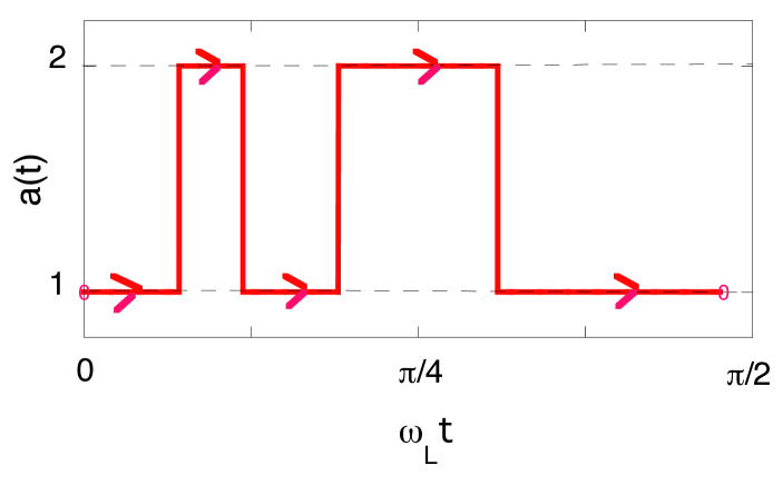
Figure 1:
Schematic diagram showing a Feynman path $a(t)$ for a spin-1/2 precessing in a magnetic field. The path connects the state $|1{\rangle}$ at $t=0$ with the same state at $t=2/\omega_{L}$. Between these times the path jumps between $1$ and $2$, passing through $|2{\rangle}$ at $t=1/\omega_{L}$.

The functional $\mathcal{F}(path)$ is given by Eq.(9) with $\beta(t^{\prime})=\delta(t^{\prime}-T/2)$,

$$\mathcal{F}(path)=\int_{0}^{t}\delta(t^{\prime}-T/2)a(t^{\prime})dt^{\prime}=a(T/2).$$ (24)

Thus, we combined the Feynman paths ending in the state $|1{\rangle}$ at $t=T$ into two virtual pathways, one containing the paths passing at $t=T/2$ through the state $|1{\rangle}$, and the other - the paths passing through the state $|2{\rangle}$. The corresponding probability amplitudes are those for evolving the spin freely from its initial state to $|1{\rangle}$ or $|2{\rangle}$ at $t=T/2$, and then to the final state $|1{\rangle}$ at $t=T$,

$$A(1)=\cos^{2}(\omega_{L}T/2){\quad}$$ (25)

$$A(2)=-\sin^{2}(\omega_{L}T/2).$$

We will need a meter. The interaction $-i\partial_{f}\delta(t-T/2)\hat{A}$ corresponds to a von Neumann measurement vN of the operator $\hat{A}=1\times|1{\rangle}{\langle}1|+2\times|2{\rangle}{\langle}2|$ performed at $t=T/2$. The accuracy of the measurement depends on the width $\Delta f$ of the initial meter’s state, which we will choose to be a Gaussian,

$$G(f)=(2/\pi\Delta f^{2})^{1/4}\exp(-f^{2}/\Delta f^{2}),{\quad}\int|G(f)|^{2}df=1.$$ (26)

It is easy to check that the average meter reading ${\langle}f{\rangle}$ in Eqs.(17) is given by

$${\langle}f{\rangle}=\frac{A(1)^{2}+2A(2)^{2}+3A(1)A(2)\exp(-0.5/\Delta f^{2})}{A(1)^{2}+A(2)^{2}+2A(1)A(2)\exp(-0.5/\Delta f^{2})},$$ (27)

its dependence on $\Delta f$ shown in Fig.2.

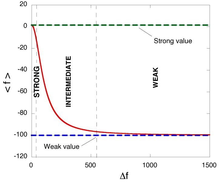
Figure 2: The mean meter reading as the function of the accuracy of the measurement in the double-slit case of the Sect. IX. In the strong measurement regime the meter destroys coherence between the pathways passing through different slits, but also destroys the interference pattern. In the weak regime the interference is intact, but the measured mean slit number is $-100$. In the intermediate regime the mean slit number changes smoothly from $1.5$ to $-100$.

This is, of course, an oversimplified version of the Young’s double slit experiment: the states at $t=T/2$ play the role of the two slits, and the states at $t=T$ - the role of the positions on the screen where an ’interference pattern’ is observed.
Consider first a ’strong’ measurement of the slit number. Choose the final time such that finding the freely precessing spin in the state $|1{\rangle}$ is unlikely (our ’interference pattern’ has there a minimum, or a ’dark fringe’), say $T=\arccos(1/203)/\omega_{L}\approx 1.5659/\omega_{L}$. Sending $\Delta f\to 0$, for the probability distribution of the meter’s readings we have [cf. Eq.(14)]

$$P^{1\leftarrow 1}(T|f)=\cos^{4}(\omega_{L}T/2)\delta(f-1)+\sin^{4}(\omega_{L}T/2)\delta(f-2)$$ (28)

$$\approx 0.252\delta(f-1)+0.248\delta(f-2).$$

We observe that the two pathways are travelled with almost equal probability, and Eq.(27) gives us the mean slit number

$${\langle}f{\rangle}_{strong}\approx 1.5.$$

However, this is not the original spin precession we set out to study. The interference pattern has been destroyed and the probability to arrive at the final position $|1{\rangle}$, which without a meter was

$$|A(1)+A(2)|^{2}\approx 0.000024,$$ (29)

is now close to $0.5$. This is a textbook example which illustrates the Uncertainty Principle: converting virtual paths into real ones comes at the cost of loosing the interference pattern.

Not satisfied, we try to minimise the perturbation in the hope to learn something about the route chosen by the system with the interference intact. We send $\Delta f$ to infinity, and after many trials obtain the answer: the mean number of the slit used is

$${\langle}f{\rangle}_{weak}=Re\frac{1\times A(1)+2\times A(2)}{A(1)+A(2)}=-100.$$ (30)

Which brings us back to our original question, to rephrase the title of Ref.W1 , ”How the result of measuring the number of the slit in a double slit experiment can turn out to be $-100$?”

X Conclusions and discussion

We have tried to evaluate the mean number of the slit a particle goes through in a double slit experiment, and came up with the number $-100$. The mathematics is straightforward, and we need to understand the meaning of this result before employing the ’weak measurements’ elsewhere. There are just two slits, numbered $1$ and $2$, so the result looks a bit strange. Has our measurement gone wrong, or is the quantum world so strange that there are slits we are not aware of? We opt for the first choice.

Wrong measurements are common in classical physics. They can be made and repeated, but only have meaning within the narrow context of the wrong experiment itself. A broken speedometer will read $50$ m.p.h each time the car goes at $100$ m.p.h, and might convince the driver, but not the traffic policemen who stops him for speeding. The slit number $-100$ may come up in a weak measurement, but cannot be used for any other purpose, such as convincing a potential user that the screen he is about to buy has more than two holes drilled in it.
There is, however, one important distinction. Classically, one can always find the right answer and correct, or re-calibrate the errant speedometer. Quantally, it is not so. According to the Uncertainty Principle, there is no correct answer to the question asked. The nearest classical analogy might be this. Suppose a (purely classical) charge can be transferred across one of the two lead wires, and an observer can measure, which one has been chosen. Then the wires are heated up and melted into one. Which of the two wires has the charge gone through now? This is what interference does, it ’melts’ the pathways through the two slits into a single one, thus depriving the ’Which way?’ question of its meaning.
Having started to use analogies it is difficult to stop. Here is the last one: one asks a manager a question the said manager is unable or unwilling to answer properly. Yet an answer he/she must give. The answer (or no-answer) given will have little to do with what one wants to know. It will be repeated should the question be asked again. It shouldn’t, however, be used to draw further conclusions about the matter of interest.
The ’weak measurements’ rely on an interesting interference effect which has applications beyond measurement theory HART , LAM . They can be made, and have been made in practice W2 . They have useful applications in interferometry W7 ; W8 . However, their results should not be over-interpreted. Bizarre weak values indicate the failure of a measurement procedure under the conditions where, according to the Uncertainty Principle, it must fail. Seen like this, the ’ weak measurements’ loose much of their original appeal, and the calculation of ’weak values’ reduces to a simple exercise in first order perturbation theory.
Finally, throughout the paper we appealed to the Uncertainty Principle, seen as one of the basic axioms of quantum theory. It is possible that the Principle itself will be explained in simpler terms within a yet unknown general theory. However, we argue, that the weak measurements have not yet given such an explanation, nor provided any deeper insight into physical reality.

- (1) Aharonov Y, Albert DZ, Vaidman L. How the result of a measurement of a component of the spin of a spin- particle can turn out to be 100. Physical Review Letters 1988; 60 (14): 1351–1354. http://dx.doi.org/10.1103/PhysRevLett.60.1351
- (2) Duck IM, Stevenson PM, Sudarshan ECG. The sense in which a “weak measurement” of a spin- particle’s spin component yields a value 100. Physical Review D 1989; 40 (6): 2112–2117. http://dx.doi.org/10.1103/PhysRevD.40.2112
- (3) Ritchie NWM, Story JG, Hulet RG. Realization of a measurement of a “weak value”. Physical Review Letters 1991; 66 (9): 1107–1110. http://dx.doi.org/10.1103/PhysRevLett.66.1107
- (4) Aharonov Y, Vaidman L. The two-state vector formalism of quantum mechanics. In: Time in Quantum Mechanics, Muga G, Mayato RS, Egusquiza I (editors), Springer, 2002, pp.369–412. http://arxiv.org/abs/quant-ph/0105101
- (5) Aharonov Y, Botero A, Popescu S, Reznik B, Tollaksen J. Revisiting Hardy’s paradox: counterfactual statements, real measurements, entanglement and weak values. Physics Letters A 2002; 301: 130–138. http://arxiv.org/abs/quant-ph/0104062
- (6) Jozsa R. Complex weak values in quantum measurement. Physical Review A 2007; 76 (4): 044103. http://arxiv.org/abs/0706.4207
- (7) Dixon PB, Starling DJ, Jordan AN, Howell JC. Ultrasensitive beam deflection measurement via interferometric weak value amplification. Physical Review Letters 2009; 102 (17): 173601. http://arxiv.org/abs/0906.4828
- (8) Popescu S. Weak measurements just got stronger. Physics 2009; 2: 32. http://dx.doi.org/10.1103/Physics.2.32
- (9) Dressel J, Jordan AN. Sufficient conditions for uniqueness of the weak value. Journal of Physics A: Mathematical and Theoretical 2012; 45 (1): 015304. http://arxiv.org/abs/1106.1871
- (10) Rozema LA, Darabi A, Mahler DH, Hayat A, Soudagar Y, Steinberg AM. Violation of Heisenberg’s measurement-disturbance relationship by weak measurements. Physical Review Letters 2012; 109 (10): 100404. http://dx.doi.org/10.1103/PhysRevLett.109.100404
- (11) Palmer J. Heisenberg uncertainty principle stressed in new test. BBC News: Science & Environment. Publication date: 7 September 2012; http://www.bbc.co.uk/news/science-environment-19489385
- (12) Leggett AJ. Comment on “How the result of a measurement of a component of the spin of a spin- particle can turn out to be 100”. Physical Review Letters 1989; 62 (19): 2325–2325. http://dx.doi.org/10.1103/PhysRevLett.62.2325
- (13) Peres A. Quantum measurements with postselection. Physical Review Letters 1989; 62 (19): 2326–2326. http://dx.doi.org/10.1103/PhysRevLett.62.2326
- (14) Sokolovski D. Weak values, “negative probability,” and the uncertainty principle. Physical Review A 2007; 76 (4): 042125. http://arxiv.org/abs/0905.3810
- (15) Sokolovski D, Puerto Giménez I, Sala Mayato R. Feynman-path analysis of Hardy’s paradox: Measurements and the uncertainty principle. Physics Letters A 2008; 372 (21): 3784–3791. http://arxiv.org/abs/0903.4795
- (16) Sokolovski D, Puerto Giménez I, Sala Mayato R. Path integrals, the ABL rule and the three-box paradox. Physics Letters A 2008; 372 (44): 6578–6583. http://arxiv.org/abs/0903.4600
- (17) Parrott S. Quantum weak values are not unique. What do they actually measure? 2009; http://arxiv.org/abs/0909.0295
- (18) Feynman RP, Leighton RB, Sands M. The Feynman Lectures on Physics, Volume 3. Reading, Massachusetts: Addison-Wesley, 1965.
- (19) Bohm D. Quantum Theory. New York: Dover Publications, 1989., p. 600.
- (20) Sokolovski D. Path integral approach to space-time probabilities: A theory without pitfalls but with strict rules. Physical Review D 2013; 87 (7): 076001. http://arxiv.org/abs/1301.1244
- (21) von Neumann J. Mathematical Foundations of Quantum Mechanics. Investigations In Physics, Beyer RT (translator), Princeton: Princeton University Press, 1955, pp.183–217.
- (22) Sokolovski D, Baskin LM. Traversal time in quantum scattering. Physical Review A 1987; 36 (10): 4604–4611. http://dx.doi.org/10.1103/PhysRevA.36.4604
- (23) Sokolovski D, Akhmatskaya E. Hartman effect and weak measurements that are not really weak. Physical Review A 2011; 84 (2): 022104. http://arxiv.org/abs/1103.5620
- (24) Monks PDD, Xiahou C, Connor JNL. Local angular momentum-local impact parameter analysis: Derivation and properties of the fundamental identity, with applications to the F + H2, H + D2, and Cl + HCl chemical reactions. Journal of Chemical Physics 2006; 125 (13): 133504-133513. http://dx.doi.org/10.1063/1.2210480