Symmetric and asymmetric solitons in dual-core couplers with competing quadratic and cubic nonlinearities

Abstract

We consider the model of a dual-core spatial-domain coupler with $\chi^{(2)}$ and $\chi^{(3)}$ nonlinearities acting in two parallel cores. We construct families of symmetric and asymmetric solitons in the system with self-defocusing $\chi^{(3)}$ terms, and test their stability. The transition from symmetric to asymmetric soliton branches, and back to the symmetric ones proceeds via a bifurcation loop. A pair of stable asymmetric branches emerge from the symmetric family via a supercritical bifurcation; eventually, the asymmetric branches merge back into the symmetric one through a reverse bifurcation. The existence of the loop is explained by means of an extended version of the cascading approximation for the $\chi^{(2)}$ interaction, which takes into regard the XPM par of the $\chi^{(3)}$ interaction. When the inter-core coupling is weak, the bifurcation loop features a concave shape, with the asymmetric branches losing their stability at the turning points. In addition to the two-color solitons, which are built of the fundamental-frequency (FF) and second-harmonic (SH) components, in the case of the self-focusing $\chi^{(3)}$ nonlinearity we also consider single-color solitons, which contain only the SH component but may be subject to the instability against FF perturbations. Asymmetric single-color solitons are always unstable, whereas the symmetric ones are stable, provided that they do not coexist with two-color counterparts. Collisions between tilted solitons are studied too.

OCIS numbers: 190.6135; 190.2620; 230.4320

I Introduction

The effect of the second-harmonic (SH) generation by monochromatic light was first demonstrated in 1961 Franken , and has been a topic of great interest ever since Torner ; New . The work on this theme includes many studies dealing with solitons supported by the quadratic ($\chi^{(2)}$) nonlinearity review1 ; review2 . While the $\chi^{(2)}$ interactions between the fundamental-frequency (FF) and SH fields are sufficient for the creation of solitons, the competition between the $\chi^{(2)}$ nonlinearity and its cubic ($\chi^{(3)}$) counterpart, either self-focusing or defocusing, may be an essential factor affecting the efficiency of the FF $\rightleftarrows$ SH conversion. In addition to the material Kerr effect, it was predicted A ; F and experimentally demonstrated E ; Ady that $\chi^{(3)}$ nonlinearity can be engineered by means of the quasi-phase-matching (QPM) technique, which makes it possible to control the modulational instability C and pulse compression H in the medium. The $\chi^{(3)}$ nonlinearity may also be induced by semiconductor dopants implanted into the $\chi^{(2)}$ material semi1 -semi3 .

Effects of competing $\chi^{(2)}:\chi^{(3)}$ nonlinearities on spatial solitons were analyzed in detail Komissarova -B . It was predicted that stable two-color solitons, built of the FF and SH components, exist in media with the self-defocusing sign of the cubic nonlinearity, where the solitons do not exist in the absence of the $\chi^{(2)}$ interactions Buryak-Kivshar-Trillo-95 . It has also been shown that the self-focusing $\chi^{(3)}$ term supports single-color solitary waves built solely of the SH component, but they are prone to destabilization by the $\chi^{(2)}$ interactions. In fact, the single-color solitons are always unstable when they coexist with the two-color ones Bang-Kivshar-Buryak-98 .

The soliton dynamics in symmetric dual-core systems, alias couplers, has also drawn a great deal of attention, starting from the analysis of solitons and their bifurcations in the model of twin-core optical fibers with the intra-core Kerr nonlinearity fibers1 -fibers6 , which was recently followed by the consideration of the soliton stability in the coupler combining the Kerr terms with the parity-time ($\mathcal{PT}$) symmetry, represented by equal gain and loss coefficients in the coupled cores PT1 ; PT2 . A similar analysis was reported for spatial solitons in planar dual-core symmetric waveguides with intrinsic $\chi^{(2)}$ nonlinearity Mak-Malomed-Chu-97 ,Mak-Malomed-Chu-98 . In all the cases, the increase of the total energy or power of the soliton (in the temporal or spatial domain, respectively) leads to the symmetry-breaking bifurcation (SBB), the difference being that the bifurcation is subcritical or supercritical in the couplers with the $\chi^{(3)}$ and $\chi^{(2)}$ nonlinear terms, respectively. These bifurcations are important examples of the phenomenology of the spontaneous symmetry breaking of localized modes in nonlinear media Springer .

These findings suggest one to consider dual-core systems with competing self-focusing and self-defocusing nonlinearities, where the increase of the total power may, at first, convert symmetric solitons into asymmetric ones through the SBB, which is followed, at larger powers, by an inverse symmetry-restoring bifurcation (SRB), if the self-defocusing dominates at high powers. A natural model of this type is based on the coupler with a combination of self-focusing cubic and self-defocusing quintic intra-core nonlinear terms Albuch-Malomed-07 . The analysis has demonstrated the existence of the corresponding bifurcation loops. A similar effect was demonstrated in an allied model, based on the nonlinear Schrödinger equation including the combination of the cubic-quintic (CQ) terms and a double-well potential, which represents a double-channel trapping structure built into the single waveguide Zeev . Dynamical switching between channels in the latter system was studied too Radik . These results suggest that couplers with competing nonlinearities have a potential for applications to all-optical data processing.

Saturable nonlinearity is somewhat similar to the combination of the competing CQ terms. In this context, it is relevant to refer to earlier works which analyzed the SBB and dynamical switching of solitons in the coupler with the saturable intra-core nonlinearity sat1 -sat4 . However, that system does not give rise to bifurcation loops, as it does not feature a switch between the self-focusing and defocusing with the increase of power.

The above-mentioned $\chi^{(2)}:\chi^{(3)}$ combination of interactions is another natural setting for the realization of the coupler with competing intra-core nonlinearities. In fact, this setting is more realistic for experimental realization, as it is not easy to find photonic materials demonstrating a dominant quintic term without conspicuous losses, while the self-defocusing $\chi^{(3)}$ terms may be induced by means of the above-mentioned techniques. The study of both two- and single-color solitons, their stability, bifurcations, and interactions in such a system is the subject of the present work. The model is formulated in Section II. The main results, in the form of bifurcation diagrams (which feature the loops) for two-color solitons in the model with the self-defocusing $\chi^{(3)}$ nonlinearity, are reported in Section III. In addition to systematic numerical results, we also propose a qualitative explanation of the existence of the loop, and its collapse which occurs with the increase of the strength of the linear coupling between the cores, based on the cascading approximation for the $\chi^{(2)}$ interaction, to which the $\chi^{(3)}$-induced XPM (cross-phase-modulation) interaction is added. In Section III, we also consider spontaneous transformation of unstable solitons into breathers, and collisions between moving (spatially tilted) stable ones. Results for single-color (SH) solitons in the system with the self-focusing $\chi^{(3)}$ terms are produced in Section IV. The paper is concluded by Section V.

II The model

We consider the co-propagation of the FF and SH fields, $u_{1,2}(x,z)$ and $w_{1,2}(x,z)$, in the symmetric coupler (subscripts $1$ and $2$ pertain to its two cores), with the combined $\chi^{(2)}:\chi^{(3)}$ nonlinearity in its cores. The setting, that does not include losses and spatial walkoff (which are negligible for relatively short propagation distances available to the experiment), is described by the system of linearly-coupled propagation equations in the spatial domain, which can be readily derived as a combination of those introduced earlier in Refs. Buryak-Kivshar-Trillo-95 ; G ; Bang-Kivshar-Buryak-98 ; Ady and Mak-Malomed-Chu-97 ; Mak-Malomed-Chu-98 :

$$iu_{1z}+u_{1xx}+u_{1}^{\ast}w_{1}+\sigma\left(\frac{1}{4}\left|u_{1}\right|^{2}+2\left|w_{1}\right|^{2}\right)u_{1}+Qu_{2} = 0,$$

$$2iw_{1z}+w_{1xx}-\alpha w_{1}+\frac{1}{2}u_{1}^{2}+\sigma\left(4\left|w_{1}\right|^{2}+2\left|u_{1}\right|^{2}\right)w_{1}+Kw_{2} = 0,$$

$$iu_{2z}+u_{2xx}+u_{2}^{\ast}w_{2}+\sigma\left(\frac{1}{4}\left|u_{2}\right|^{2}+2\left|w_{2}\right|^{2}\right)u_{2}+Qu_{1} = 0,$$

$$2iw_{2z}+w_{2xx}-\alpha w_{2}+\frac{1}{2}u_{2}^{2}+\sigma\left(4\left|w_{2}\right|^{2}+2\left|u_{2}\right|^{2}\right)w_{2}+Kw_{1} = 0,$$

Here $\alpha$ represents the phase mismatch between the FF and SH waves, $\sigma=+1$ or $-1$ determines, respectively, the self-focusing or defocusing sign of the $\chi^{(3)}$ nonlinearity ($|\sigma|=1$ can be fixed by scaling), while $Q$ and $K$ are inter-core coupling constants for the FF and SH fields. The total power (norm) of the fields in each core is

$$P_{1,2}=\int_{-\infty}^{+\infty}\left[\left|u_{1,2}(x)\right|^{2}+4\left|w_{1,2}(x)\right|^{2}\right]dx,$$ (2)

the conserved power being $P\equiv P_{1}+P_{2}$.

Stationary soliton solutions with propagation constant $\lambda$ are looked for as

$$\left\{u_{1}\left(x,z\right),w_{1}\left(x,z\right)\right\} = \left\{U_{1}\left(x\right),W_{1}\left(x\right)\right\}e^{i\lambda z},$$

$$\left\{u_{2}\left(x,z\right),w_{2}\left(x,z\right)\right\} = \left\{U_{2}\left(x\right),W_{2}\left(x\right)\right\}e^{2i\lambda z},$$

where real functions $U_{1,2}(x)$ and $W_{1,2}(x)$ satisfy the following equations:

$$-\lambda U_{1}+U_{1}^{\prime\prime}+U_{1}^{\ast}W_{1}+\sigma\left(\frac{1}{4}\left|U_{1}\right|^{2}+2\left|W_{1}\right|^{2}\right)U_{1}+QU_{2} = 0,$$

$$-\left(4\lambda+\alpha\right)W_{1}+W_{1}^{\prime\prime}+\frac{1}{2}U_{1}^{2}+\sigma\left(4\left|W_{1}\right|^{2}+2\left|U_{1}\right|^{2}\right)W_{1}+KW_{2} = 0,$$

$$-\lambda U_{2}+U_{2}^{\prime\prime}+U_{2}^{\ast}W_{2}+\sigma\left(\frac{1}{4}\left|U_{2}\right|^{2}+2\left|W_{2}\right|^{2}\right)U_{2}+QU_{1} = 0,$$

$$-\left(4\lambda+\alpha\right)W_{2}+W_{2}^{\prime\prime}+\frac{1}{2}U_{2}^{2}+\sigma\left(4\left|W_{2}\right|^{2}+2\left|U_{2}\right|^{2}\right)W_{2}+KW_{1} = 0,$$

with the prime standing for $d/dx$. These equations were solved numerically by means of the Newton-Raphson method based on a finite-difference scheme. The asymmetry of solitons with unequal amplitudes in the two cores, $\left(U_{1,2}\right)_{\max}$ and $\left(V_{1,2}\right)_{\max}$, is measured by

$$\mathrm{\Theta}_{\mathrm{F}}=\frac{\left(U_{1}\right)_{\max}^{2}-\left(U_{2}\right)_{\max}^{2}}{\left(U_{1}\right)_{\max}^{2}+\left(U_{2}\right)_{\max}^{2}}.$$ (5)

This parameter is defined in terms of the FF component only, as its amplitudes in the two-color solitons are always essentially larger than the SH amplitudes.

The stability of the soliton solutions was investigated by means of direct simulations of the perturbed evolution within the framework of Eqs. (LABEL:eqs). The simulations were carried out using the fourth-order Runge-Kutta algorithm.

The bifurcation loops are produced in the next section for $\sigma=-1,$ i.e., the self-defocusing sign of the $\chi^{(3)}$ nonlinearity. This choice is necessary, once we aim to consider the competing nonlinear interactions, $\chi^{(2)}$ (effectively self-focusing, in the cascading limit Torner ) and $\chi^{(3)}$. Most results will be presented for $\alpha=0.5$, as this value of the mismatch adequately represents the generic situation. However, some essential findings (the critical size of the coupling, $Q_{\mathrm{cr}}$, at which the bifurcation loop shrinks to zero) are included too for other values of $\alpha$.

The parameters are different in Section IV dealing with single-color solitons. In particular, $\sigma=+1$ is fixed in that case, as such solitons exist only for the self-focusing $\chi^{(3)}$ nonlinearity.

III Bifurcation diagrams and dynamics of two-color solitons

III.1 The bifurcation loops

Because the asymmetry of the solitons produced by the SBB, defined as per Eq. (5), is their most important characteristic, the bifurcation diagrams were generated by varying propagation constant $\lambda$ and plotting the respective results in the form of $\mathrm{\Theta}_{\mathrm{F}}$ [see Eq. (5)] vs. the total power, $P$, at fixed values of the FF coupling constant, $Q$, and for $K=0$. The latter assumption is relevant, as the evanescent field, which accounts for the inter-core coupling, decays faster in the SH component. In fact, results were also obtained for $K\neq 0,$ showing slight additional shrinkage of the bifurcation loops displayed in Figs. 1 and 2. For instance, for the same values of $Q=0.0054$ and $\alpha=0.5$, which correspond to Fig. 1(b), the increase of $K$ from zero to $0.0040$ leads to a decrease of the largest power at which the asymmetric solitons exist by $\approx 9\%$.

Figures 1 and 2 demonstrate the bifurcation loops of two different types: concave and convex, at smaller and larger values of $Q$, respectively. The increase of $Q$ leads to the shrinkage of the loop, which vanishes (“collapses”), for $\alpha=0.5$, at $Q_{\mathrm{cr}}\approx 0.0117$.

Figure 1: (Color online) Concave bifurcation loops for solitons, obtained at different values of the FF inter-core coupling coefficient $Q$, are displayed by means of the dependence of asymmetry measure (5) on the total power (norm), $P$: (a) $Q=0.0047$, (b) $Q=0.0054$, (c) $Q=0.0065$, (d) $Q=0.0085$. Here and in the next figure, as well in Fig. 11 below, stable and unstable portions of the solution branches are shown by solid and dashed-dotted segments, respectively. The dot on the unstable asymmetric branch indicates a solution whose spontaneous transformation into a symmetric breather is displayed below in Fig. 4. This figure and ones following below are drawn for $\alpha=0.5$.

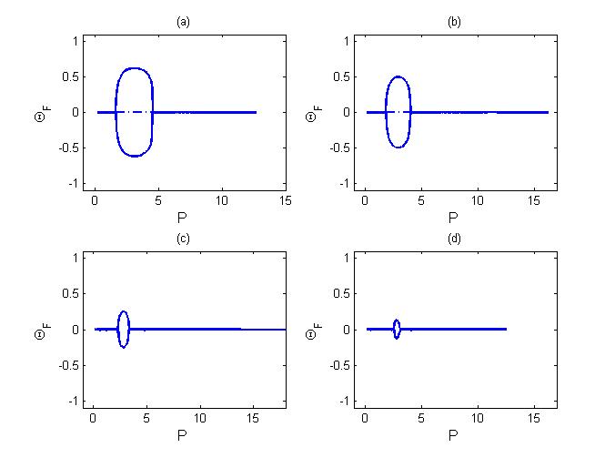
Figure 2: (Color online) The continuation of Fig. (1) – convex bifurcation loops obtained at larger values of the FF coupling constant: (a) $Q=0.0098$, (b) $Q=0.0106$, (c) $Q=0.0115$, (d) $Q=0.0117$. In panels (c) and (d), the short unstable segment of the symmetric solitons inside the loops is not plotted.

We have also performed the analysis for other values of the mismatch. The results are summarized in Fig. 3, in the form of curve $Q_{\mathrm{cr}}(\alpha)$, which is displayed along with qualitative estimate (10) derived below.

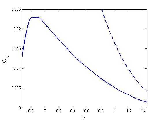
Figure 3: (Color online) The solid curve shows the numerically found critical value of the FF coupling constant, $Q_{\mathrm{cr}}$, at which the bifurcation loop collapses, versus the phase mismatch, $\alpha$. The dashed-dotted curve represents the crude analytical approximation for $Q_{\mathrm{cr}}$ given by Eq. (10).

The concave bifurcation loop connects the symmetry-breaking and restoring bifurcations of the super- and subcritical types, respectively, while both bifurcations are supercritical if they are connected by a convex loop. In agreement with the general principles of the bifurcation theory book ; Springer , segments of the branches of asymmetric solitons in the concave loop, which connect the point of the supercritical SBB with the turning points, are stable, while the segments which link the turning points to the point of the subcritical SRB are unstable. As might be expected too, the branches of the symmetric solitons, corresponding to $\mathrm{\Theta}_{\mathrm{F}}\equiv 0$ in Figs. 1 and 2, are unstable inside the loop, and stable outside.

III.2 The analytical approximation

Basic properties of the bifurcation loop can be qualitatively explained by means of an extended form of the well-known cascading approximation, which is used to eliminate (“enslave”) the SH field in favor of the FF, when the mismatch is large and the diffraction term may be neglected in the equations for the SH Torner ; review1 ; review2 (a more sophisticated version of the cascading approximation, which makes use of the Fourier decomposition of periodic structures, was developed in Refs. A ; F ; C for systems based on QPM gratings). This approximation implies that the amplitude of the SH field is much smaller than its FF counterpart, hence, applying the approximation to the SH equations in system (LABEL:eqs-stationary-substitution), it is necessary to take the XPM term into account. Thus, the cascading limit yields, in the present case,

$$W_{n}(x)\approx\frac{\left(U_{n}(x)\right)^{2}}{2\left[\alpha+2\left|U_{n}(x)\right|^{2}\right]},~{}n=1,2,$$ (6)

where, as said above, we set $\sigma=-1$. Then, the substitution of this expression into the FF equations of system (LABEL:eqs-stationary-substitution) yields a pair of linearly coupled equations with an effective saturable nonlinearity:

$$-\lambda U_{1}+U_{1xx}+\frac{\left|U_{1}\right|^{2}}{2\left(\alpha+2\left|U_{1}\right|^{2}\right)}U_{1}-\frac{1}{4}\left|U_{1}\right|^{2}U_{1}+QU_{2} = 0,$$

$$-\lambda U_{2}+U_{2xx}+\frac{\left|U_{2}\right|^{2}}{2\left(\alpha+2\left|U_{2}\right|^{2}\right)}U_{2}-\frac{1}{4}\left|U_{2}\right|^{2}U_{2}+QU_{1} = 0.$$

Unlike the system of coupled equations with the cubic nonlinearity fibers1 -fibers6 , the SBB point cannot be found in an exact form in this model. However, for a crude estimate one may treat it as cubic system with effective coefficients

$$\left(\chi_{1,2}^{(3)}\right)_{\mathrm{eff}}=\frac{1}{2}\left[\frac{1}{\alpha+2\left(U_{1,2}\right)_{\max}^{2}}-\frac{1}{2}\right],$$ (8)

taken at the soliton’s center. After that, the application of the well-known exact result for the SBB point in the cubic system fibers1 to the system with coefficients (8) yields and equation which predicts the peak power of the symmetric solitons at the bifurcation points, $P_{\max}\equiv U_{\max}^{2}$:

$$P_{\max}^{2}+\left(\frac{16Q}{3}-1+\frac{\alpha}{2}\right)P_{\max}+\frac{8}{3}\alpha Q=0.$$ (9)

Obviously, too roots of this quadratic equation correspond to the SBB and SRB points bounding the bifurcation loop. Further, in the framework of the present approximation, the above-mentioned critical value of the coupling constant, $Q_{\mathrm{cr}}$, at which the loop collapses, i.e., the SBB and SRB points merge into one, is identified as a value of $Q$ at which the discriminant of Eq. (9) vanishes. The latter condition readily leads to the following result:

$$Q_{\mathrm{cr}}=\frac{3}{32}\left(\sqrt{2}-\sqrt{\alpha}\right)^{2}.$$ (10)

As seen in Fig. 3, the analytical result strongly overestimates the actual values of $Q_{\mathrm{cr}}$ (which is not surprising, as the analysis is quite coarse), but, nevertheless, the approximation provides an explanation of the existence of the bifurcation loop, as well as the trend of $Q_{\mathrm{cr}}$ to decrease with the increases of $\alpha$ at $\alpha>0$. The decrease of the discrepancy with the increase of the mismatch, $\alpha$, is a natural feature of the cascading approximation.

III.3 Transformations of unstable solitons

Direct numerical simulations demonstrate that the unstable symmetric solitons evolve towards breathers oscillating around either of the stable asymmetric soliton existing at the same total power (not shown here in detail, as the picture is similar to that observed in previously studied models). This transition gives rise to very little radiation loss, i.e., the dynamical symmetry breaking practically keeps the initial total power.

More interesting is the spontaneous transformation of asymmetric solitons belonging to the unstable segments of the concave loop, which is a specific feature of the present setting, see Fig. 1. An example, displayed in Fig. 4, demonstrates that these unstable solitons spontaneously evolve into breathers, which are symmetric on the average, with the fields in the two cores oscillating out of phase, as shown in Fig. 5. Overall, this effect may be considered as dynamical resymmetrization of the solitons. This transition also conserves the initial power of the unstable soliton almost exactly, and the emerging breathers emit virtually no radiation waves.

Figure 4: (Color online) The evolution, initiated by small perturbations, of the FF and SH components in cores 1 and 2 (left and right panels, respectively) of the unstable asymmetric soliton marked by the dot in Fig. 1(a), with $Q=0.0047$, propagation constant $\lambda=0.0255$, and total power $P=15.77$. In each panel, the plots of the FF and SH components are juxtaposed with a shift, for the purpose of clearer presentation.

Figure 5: (Color online) Periodic out-of-phase oscillations of amplitudes of the FF fields in the two cores, corresponding to the situation displayed in Fig. 4.

III.4 Collisions between two-color solitons

Equations (LABEL:eqs) are obviously invariant with respect to the spatial tilt, which is a counterpart of the Galilean boost in the temporal domain:

$$u_{1,2}(x,z) \rightarrow u_{1,2}\left(x-cz,z\right)\exp\left(\frac{i}{2}cx-\frac{i}{4}c^{2}z\right),$$

$$w_{1,2}(x,z) \rightarrow w_{1,2}\left(x-cz,z\right)\exp\left(icx-\frac{i}{2}c^{2}z\right),$$ (11)

where $c$ is an arbitrary real tilt constant. This invariance makes it natural to consider collisions between spatial solitons tilted in opposite directions. Direct simulations of the collisions make it possible to draw the following conclusions.

At low powers, the collisions are, as might be expected, nearly elastic, and do not affect tracks of the two beams, see an example in Fig. 6 for a pair of identical stable symmetric solitons. At higher powers, the collisions are inelastic. An example, this time for asymmetric solitons, is shown in Fig. 7, where larger components in both solitons belong to the same core. In this case, the collision leads to splitting of the two solitons into multiple pulses. In addition, Fig. 8 displays an example of the inelastic collision between strongly asymmetric solitons which are specular counterparts to each other, with the larger components belonging to different cores. In the latter case, the collision tends to transform the solitons into more symmetric ones.

Figure 6: (Color online) The elastic collision between low-power solitons, for $Q=0.003$ and $\lambda=0.0046$ (which corresponds to total power $P=0.5162$). In this figure and similar ones which display collisions, the left and right plots represent, respectively, the FF fields in cores 1 and 2. The picture of the SH component is quite similar.

Figure 7: (Color online) The inelastic collision between identical high-power asymmetric solitons, at $Q=0.003$ and $\lambda=0.0248$ (which corresponds to total power $P=10.43$).

Figure 8: (Color online) The inelastic collision between strongly asymmetric solitons, one being a mirror image of the other (i.e., the larger component of one soliton collides with the smaller component of the other), for $Q=0.003$ and $\lambda=0.0245$, which corresponds to total power $P=5.63$.

Lastly, collisions between high-power symmetric solitons, which are located to the right of the bifurcation loops, in terms of Figs. 1 and 2, are strongly inelastic too. An example, displayed in Fig. 9, may be roughly interpreted as transformation of the two colliding solitons into three, which emerge in strongly excited states, while the spatial symmetry of the configuration persists after the collision.

Figure 9: (Color online) The inelastic collision between identical symmetric solitons whose power exceeds the largest power of asymmetric ones, i.e., they are located to the right of the bifurcation loop, in terms of Figs. 1 and 2. The parameters are $Q=0.003$, $\lambda=0.0267$, and $P=10.99$.

IV Single-color (second-harmonic) solitons

To allow the existence of single-color SH solitons in the model with the self-focusing $\chi^{\left(3\right)}$ terms, i.e., $\sigma=+1$ in Eqs. (LABEL:eqs), it is necessary to include the inter-core coupling of the SH fields, $K$. Therefore, we here fix $Q=0.2$ and $K=0.5$. In fact, the particular value of $Q$ is not crucially important in the present context, where the FF fields are essential for the destabilization of the SH solitons. This instability is not strongly affected by the linear coupling between the FF fields in the two cores.

Figure 10 demonstrates a set of soliton shapes obtained from Eqs. (LABEL:eqs-stationary-substitution), which illustrate the transition from (asymmetric) two-color solitons [panels (a,b) and (c,d)] to the single-color symmetric one [panels(e,f)] with the decrease of the total power. The numerical investigation demonstrates that this transition occurs at $\alpha>\alpha_{\min}$ $\approx$ $-1.8$. It has been inferred that the single-color solitons are stable precisely at those values of the propagation constant, $\lambda$ [see Eq. (LABEL:eqs-stationary)], at which neither symmetric nor asymmetric two-color solitons exist, which implies the absence of the drive for the parametric instability of the SH mode against excitation of FF perturbations.

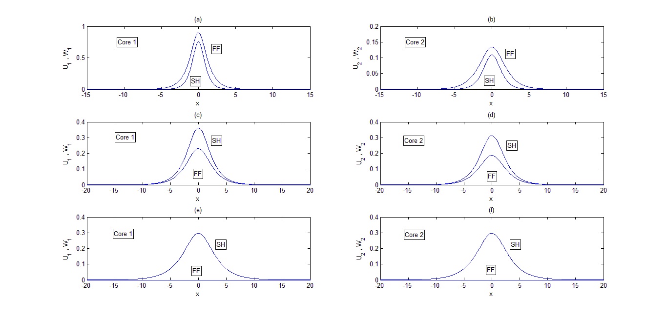
Figure 10: (Color online) The transition from two-color solitons in (a,b) and (c,d), with the dominant FF or SH components, respectively, the to the single-color (SH) soliton in panels (e,f), in the system with the self-focusing $\chi^{(3)}$ nonlinearity ($\sigma=+1$), relatively strong inter-core coupling in the SH field ($Q=0.2$, $K=0.5$), and mismatch $\alpha=-1.3$. The propagation constants of the solitons and powers of their components are: $\lambda=0.1$,$~{}\left(P_{u}\right)_{1}=1.5688$, $\left(P_{w}\right)_{1}=0.3328$, $\left(P_{u}\right)_{2}=0.0523$, $\left(P_{w}\right)_{2}=0.0956$ in (a,b); $\lambda=0.531$, $\left(P_{u}\right)_{1}=0.2027$, $\left(P_{w}\right)_{1}=1.8684$, $\left(P_{u}\right)_{2}=0.1413$, $\left(P_{w}\right)_{2}=1.4836$ in (c,d); and $\lambda=0.494$, $\left(P_{u}\right)_{1,2}=0$, $\left(P_{w}\right)_{1,2}=1.678$ in (e,f). The two-color asymmetric soliton is stable in (a,b) and unstable in (c,d). The single-color symmetric soliton in (e,f) is located at a boundary between stable and unstable subfamilies.

At $\alpha<\alpha_{\min}$, single-color solitons appear in an asymmetric form from their two-color counterparts, also with the decrease of the total power. All the asymmetric single-color solitons are unstable. With the further decrease of the total power, they turn symmetric and, simultaneously, become stable. For example, at $\alpha=-2.32$, the FF component of the two-color soliton vanishes at $\lambda=0.847$, while the powers of the SH components in the two cores are $3.742$ and $0.8792$. With the subsequent decrease of $\lambda$ to $0.7881$, the single-color soliton becomes symmetric and stable. The latter transformation is illustrated by the SBB bifurcation for the single-color solitons, which is displayed in Fig. 11, with the corresponding asymmetry parameter defined as

$$\mathrm{\Theta}_{\mathrm{S}}=\frac{\left(W_{1}\right)_{\max}^{2}-\left(W_{2}\right)_{\max}^{2}}{\left(W_{1}\right)_{\max}^{2}+\left(W_{2}\right)_{\max}^{2}},$$ (12)

cf. definition (5) for the two-color solitons.

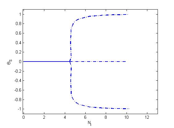
Figure 11: (Color online) The symmetry-breaking bifurcation of the single-color (SH) solitons. Asymmetry $\mathrm{\Theta}_{\mathrm{S}}$ is defined as per Eq. (12). The bifurcation takes place at $P\approx 4.47$.

An example of the evolution of unstable asymmetric single-color solitons is displayed in Fig. 12. The instability results in a very fast transformation of the soliton into its stable two-color counterpart, practically without radiative loss of the total power.

Figure 12: (Color online) The evolution of an unstable asymmetric single-color soliton at $\alpha=-2.32$, with $\lambda=0.8$ and powers in the two cores $\left(P_{w}\right)_{1}=3.0056$, $\left(P_{w}\right)_{2}=1.5616$. The left and right panels represent the fields in cores 1 and core 2, respectively. In each panel, the FF and SH components are shifted to left and right for clearer presentation.

Thus, there are two possible causes for the destabilization of the single-color SH solitons. One is the coexistence with two-color ones, which triggers the parametric instability against excitation of FF perturbations. The other instability is caused by the SBB which transforms the symmetric single-color solitons into asymmetric ones (which themselves are unstable, as shown in Fig. 11). A combined stability boundary for the single-core solitons is displayed in Fig. 13, in which the stability area is $P<P_{\max}(\alpha)$. The horizontal segment of the boundary corresponds to the SBB at $P\approx 4.47$, at which the destabilizing bifurcation happens (see Fig. 11). Obviously, this critical power does not depend on $\alpha$, as the phase mismatch amounts to a trivial shift of the SH propagation constant when the FF field is absent. On the other hand, the slanted segment with a nearly constant slope accounts for the parametric instability against the generation of the FF field, when the single-color soliton coexists with a two-color one. In all the cases, the evolution of unstable single-color solitons is quite similar to the example presented in Fig. 12.

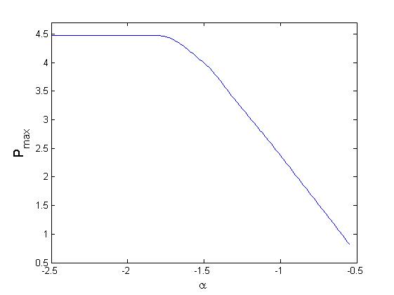
Figure 13: (Color online) The SH single-component symmetric solitons are stable with the power taking values below the maximum value shown here, $P<P_{\max}$, which depends on the phase mismatch, $\alpha$.

V Conclusion

We have introduced the model of the dual-core waveguide with the combined $\chi^{(2)}:\chi^{(3)}$ nonlinearity acting in the coupled cores. The main objective was to study the SBB-SRB (symmetry-breaking-bifurcation—symmetry-restoring-bifurcation) sequence for two-color solitons in the coupler with the competing $\chi^{(2)}$ and defocusing $\chi^{(3)}$ nonlinearities, which gives rise to the bifurcation loop. For weaker and stronger inter-core coupling, the loops feature concave and convex shapes, respectively. They shrink and disappear with the increase of the coupling constant. The existence and eventual collapse of the loop can be explained with the help of the cascading approximation for the $\chi^{(2)}$ interaction, taking into regard the $\chi^{(3)}$-induced XPM interaction. The stability of the symmetric and asymmetric solitons follows general principles of the bifurcation theory. Collisions between tilted solitons show a trend to the transition from quasi-elastic to inelastic collisions with the increase of the solitons’ power. Further, single-color SH solitons were investigated in the model with the self-focusing $\chi^{(3)}$ nonlinearity. Symmetric single-color solitons are stable, provided that they do not coexist with two-color ones, up to the SBB point of the single-color solitons.

It may be interesting to extend the analysis for the coupler carrying the three-wave system, with the Type-II $\chi^{(2)}$ interaction between two FF and one SH components, competing with the $\chi^{(3)}$ nonlinearity. A challenging problem is to extend the analysis for spatiotemporal solitons in the planar dual-core waveguide with the combined quadratic and cubic nonlinearities acting in each core.

References

- (1) P. Franken, A. E. Hill, C. W. Peters, and G. Weinreich, “Generation of Optical Harmonics”, Phys. Rev. E 7, 118-120 (1961).
- (2) G. I. Stegeman, D. J. Hagan, and L. Torner, “ cascading phenomena and their applications to all-optical signal processing, mode-locking, pulse compression and solitons”, Opt. Quant. Elect. 28, 1691-1740 (1996).
- (3) G. New, Introduction to Nonlinear Optics (Cambridge University Press: Cambridge, UK, 2011).
- (4) C. Etrich, F. Lederer, B. A. Malomed, T. Peschel, and U. Peschel, “Optical solitons in media with a quadratic nonlinearity”, Prog. Opt. 41, 483-568 (2000).
- (5) A. V. Buryak, P. Di Trapani, D. V. Skryabin, and S. Trillo, “Optical solitons due to quadratic nonlinearities: from basic physics to futuristic applications”, Phys. Rep. 370, 63-235 (2002).
- (6) C. B. Clausen, O. Bang, and Y.S. Kivshar, “Spatial solitons and induced Kerr effects in quasi-phase-matched quadratic media”, Phys. Rev. Lett. 78, 4749-4752 (1997).
- (7) O. Bang, C. B. Clausen, P. L. Christiansen, and L. Torner, “Engineering competing nonlinearities”, Opt. Lett. 24, 1413-1415 (1999).
- (8) P. Di Trapani, A. Bramati, S. Minardi, W. Chinaglia, C. Conti, S. Trillo, J. Kilius, and G. Valiulis, Focusing versus defocusing nonlinearities due to parametric wave mixing, Phys. Rev. Lett. 87, 183902 (2001).
- (9) T. Ellenbogen, A. Arie, and M. Solomon, “Noncollinear double quasi phase matching in one-dimensional poled crystal”, Opt. Lett. 32, 262-264 (2007).
- (10) M. Bache, O. Bang, W. Królikowski, J. Moses, and F. W. Wise, “Limits to compression with cascaded quadratic soliton compressors”, Opt. Express 16, 3273-3287 (2008).
- (11) J. M. Hickmann, A. S. L. Gomes, and C. B. de Araújo, “Observation of spatial cross-phase modulation effects in a self-defocusing nonlinear medium”, Phys. Rev. Lett. 68, 3547-3550 (1992).
- (12) H. Lee, W. R. Cho, J. H. Park, J. S. Kim, S. H. Park, and U. Kim, “Measurement of free-carrier nonlinearities in ZnSe based on the Z-scan technique with a nanosecond laser”, Opt. Lett. 19, 1116-1118 (1994).
- (13) M. Brambilla, L. A. Lugiato, F. Prati, L. Spinelli, and W. J. Firth, Phys. Rev. Lett. “Spatial soliton pixels in semiconductor devices79, 2042-2045 (1997).
- (14) J. F. Corney and O. Bang, “Modulational instability in periodic quadratic nonlinear materials, Phys. Rev. Lett. 87, 133901 (2001).
- (15) M. V. Komissarova and A. P. Sukhorukov, “Optical solitons in media with quadratic and cubic nonlinearities”, Bull. Russian Acad. Sci. Phys. 56, 1995-1999 (1992).
- (16) A. V. Buryak, Yu. S. Kivshar and S. Trillo, “Optical solitons supported by competing nonlinearities”, Opt. Lett. 20, 1961-1963 (1995).
- (17) O. Bang, Yu. S. Kivshar, and A. V. Buryak, “Bright spatial solitons in defocusing Kerr media supported by cascaded nonlinearities”, Opt. Lett. 22, 1680-1682 (1997).
- (18) O. Bang, “Dynamical equations for wave packets in materials with both quadratic and cubic response”, J. Opt. Soc. Am. B 14, 51 (1997).
- (19) O. Bang, Yu. S. Kivshar, A. V. Buryak, A. De Rossi and S. Trillo “Two-dimensional solitary waves in media with quadratic and cubic nonlinearity”, Phys. Rev. E 58, 5057-5069 (1998).
- (20) J. F. Corney and O. Bang, “Solitons in quadratic nonlinear photonic crystals”, Phys. Rev. E 64, 047601 (2001).
- (21) E. M. Wright, G. I. Stegeman, and S. Wabnitz, “Solitary-wave decay and symmetry-breaking instabilities in two-mode fibers”, Phys. Rev. A 40, 4455-4466 (1989).
- (22) C. Paré and M. Fłorjańczyk, “Approximate model of soliton dynamics in all-optical couplers, Phys. Rev. A 41, 6287-6295 (1990).
- (23) A. I. Maimistov, “Propagation of a light pulse in nonlinear tunnel-coupled optical waveguides”, Kvant. Elektron. 18, 758-761 [Sov. J. Quantum Electron. 21, 687-690 (1991)].
- (24) M. Romagnoli, S. Trillo, and S. Wabnitz, “Soliton switching in nonlinear couplers”, Opt. and Quant. Elect. 24, S1237-S1267 (1992).
- (25) N. Akhmediev and A. Ankiewicz, “Novel soliton states and bifurcation phenomena in nonlinear fiber couplers”, Phys. Rev. Lett. 70, 2395-2398 (1993).
- (26) P. L. Chu, B. A. Malomed, and G. D. Peng, “Soliton switching and propagation in nonlinear fiber couplers: analytical results”, J. Opt. Soc. Am. B 10, 1379-1385 (1993).
- (27) J. M. Soto-Crespo and N. Akhmediev, “Stability of the soliton states in a nonlinear fiber coupler”, Phys. Rev. E 48, 4710-4715 (1993).
- (28) B. A. Malomed, I. Skinner, P. L. Chu, and G. D. Peng, Symmetric and asymmetric solitons in twin-core nonlinear optical fibers, Phys. Rev. E 53, 4084 (1996).
- (29) R. Driben and B. A. Malomed, “Stability of solitons in parity-time-symmetric couplers”, Opt. Lett. 36, 4323-4325 (2011).
- (30) N. V. Alexeeva, I. V. Barashenkov, A. A. Sukhorukov, and Y. S. Kivshar, “Optical solitons in -symmetric nonlinear couplers with gain and loss”, Phys. Rev. A 85, 063837 (2012)
- (31) William C. K. Mak, B. A. Malomed and P. L. Chu “Solitons in coupled waveguides with quadratic nonlinearity”, Phys. Rev. E 55, 6134-6140 (1997).
- (32) William C. K. Mak, B. A. Malomed and P. L. Chu “Asymmetric solitons in coupled second-harmonic-generating waveguides”, Phys. Rev. E 57, 1092-1103 (1997).
- (33) B. A, Malomed (editor), Spontaneous Symmetry Breaking, Self-trapping, and Josephson Oscillations (Springer, 2013).
- (34) L. Albuch and B. A. Malomed “Transitions between symmetric and asymmetric solitons in dual-core systems with cubic-quintic nonlinearity”, Mathematics and Computers in Simulation, 74 (2007) 312-322.
- (35) Z. Birnbaum and B. A. Malomed, “Families of spatial solitons in a two-channel waveguide with the cubic-quintic nonlinearity”, Physica D 237, 3252-3262 (2008).
- (36) R. Driben, B. A Malomed, and P. L. Chu, “All-optical switching in a two-channel waveguide with cubic–quintic nonlinearity”, J. Phys. B: At. Mol. Opt. Phys. 39, 2455-2466 (2006).
- (37) G. D. Peng, P. L. Chu, and A. Ankiewicz, “Soliton propagation in saturable nonlinear fiber couplers – variational and numerical results”, Int. J. Nonlin. Opt. Phys. 3, 69-87 (1994).
- (38) H. Hatami-Hanza, P. L. Chu, and G. D. Peng, “Optical switching in a coupler with saturable nonlinearity”, Opt. Quant. Electr. 26, S365-S372 (1994).
- (39) A. Ankiewicz, N. Akhmediev, and G. P. Peng, “Stationary soliton states in couplers with saturable nonlinearity”, Opt. Quant. Electr. 27, 193-200 (1995).
- (40) A. Ankiewicz, N. Akhmediev, and J. M. Soto-Crespo, “Novel bifurcation phenomena for solitons in nonlinear saturable couplers”, Opt. Commun. 116, 411-415 (1995).
- (41) G. Iooss and D. D. Joseph, Elementary Stability and Bifurcation Theory (Springer: New York, 1980).