Magnetohydrostatic equilibrium. I: Three-dimensional open magnetic flux tube in the stratified solar atmosphere

Abstract

A single open magnetic flux tube spanning the solar photosphere (solar radius $\simeq R_{\odot}$) and the lower corona ($R_{\odot}+10\,{\rm Mm}$) is modelled in magnetohydrostatic equilibrium within a realistic stratified atmosphere subject to solar gravity. Such flux tubes are observed to remain relatively stable for up to a day or more, and it is our aim to apply the model as the background condition for numerical studies of energy transport mechanisms from the surface to the corona. We solve analytically an axially symmetric 3D structure for the model, with magnetic field strength, plasma density, pressure and temperature all consistent with observational and theoretical estimates. The self similar construction ensures the magnetic field is divergence free. The equation of pressure balance for this particular set of flux tubes can be integrated analytically to find the pressure and density corrections required to preserve the magnetohydrostatic equilibrium. The model includes a number of free parameters, which makes the solution applicable to a variety of other physical problems and it may therefore be of more general interest.

1 Introduction

At a radius $R_{\odot}\simeq 696\,{\rm Mm}$ from the Sun’s core its luminous surface, the photosphere, has a temperature of about $6500\,{\rm K}$. At $h\simeq 0.35-0.65\,{\rm Mm}$ above this surface the temperature falls to a minimum $T\simeq 4200\,{\rm K}$. The temperature then rises with height and experiences rapid jumps to $10^{5}\,{\rm K}$ just above $h\simeq 2\,{\rm Mm}$ and to $10^{6}\,{\rm K}$ beyond $h\simeq 2.5\,{\rm Mm}$ (Priest, 1987; Aschwanden, 2005, Ch.1, and references therein). The mechanism for the heating of the solar corona is not well understood. The atmosphere is highly active. Jets, flares, prominences and spicules carry mass and energy from the surface into the atmosphere. Although frequent and powerful, these solar accumulated events do not appear to have sufficient energy to explain the consistently high coronal temperatures.

Coronal loops, comprising strongly magnetized flux tubes, also permeate the atmosphere. Given the very low thermal pressure that resides in the solar corona the magnetic pressure can become dynamically dominant. The magnetic field may be considered as a wave guide for carrying energy from the lower solar atmosphere and releasing it as heat high in the corona. We seek to investigate such transport mechanisms with a series of numerical simulations (Shelyag et al., 2008; Fedun et al., 2009; Shelyag et al., 2009; Fedun et al., 2011; Vigeesh et al., 2012). Although transient features, these loops may persist in relative pressure equilibrium with the ambient atmosphere for many minutes, days or longer.

In this paper a magnetic flux tube is modelled in pressure balance with the surrounding atmosphere typical of the quiet Sun. Modelling a realistic magnetic flux tube in magnetohydrostatic equilibrium is challenging, particularly because of the exponential expansion in the radius of the flux tube between the photosphere and the transition region due to the drop in plasma pressure, and the additional constraint that the magnetic field should be strong enough everywhere in the corona to provide the dominant pressure. Footpoint strengths of $100\,{\rm mT}~{}(1000\,{\rm G})$ are typically observed (Zwaan, 1978; Priest, 1987; Aschwanden, 2005, and references therein, Ch.8.7, Ch.5) and models with such strong fields in pressure equilibrium are often prone to inducing unphysical negative thermal pressure (Low, 1980; Gibson & Low, 1998; Manchester et al., 2004; Gascoyne & Jain, 2009). Magnetic flux tubes appear to exhibit over-dense cores in the corona (Aschwanden et al., 2001; Winebarger et al., 2003), which would appear to conflict with hydrostatic equilibrium (Aschwanden et al., 2001; Winebarger et al., 2003). We derive an analytic expression for a set of solutions to the 3D MHD equation for pressure balance with a single open magnetic flux tube. The physical constraints on the plasma pressure, density and temperature are reasonably satisfied.

Against this background in magnetohydrostatic equilibrium, it is our intention with future work to study numerically the propagation of MHD waves through the transition region to the corona due to various physical drivers in the photosphere, with the aim of identifying the primary energy transport mechanisms. Here we describe the analytic construction of the flux tube, spanning the photosphere and about $10\,{\rm Mm}$ above the photosphere. The paper is organised as follows. Section 2.1 details the ambient atmosphere in which the magnetic flux tube will be embedded, Section 2.2 defines the structure of the magnetic flux tube, Section 2.3 outlines how the atmosphere is adjusted to balance the pressure terms, Section 2.4 considers the necessary physical constraints and in Section 3 we discuss the conclusions and opportunities presented by the model. In addition we include Appendix A, tabulating the units we use to scale the dimensionless equations, and Appendix B, containing further details of the calculations to determine the changes to the pressure and density.

2 The single open magnetic flux tube

2.1 The stratified atmosphere

Subject to many local fluctuations, eruptions and various events on different scales, and varying in time depending on the stage of the solar cycle, the atmosphere around the solar surface may nevertheless be regarded as predominantly in global hydrostatic equilibrium between solar gravity and the total pressure gradient.

Although accurate measurement of the atmospheric parameters is challenging, due to the relatively weak intensity of the emissions from the low density plasma, a number of attempts to model its structure from the observational data have been recorded. For our model we combine the results of Vernazza et al. (1981, Table 12,VALIIIC) and McWhirter et al. (1975, Table 3) for the chromosphere and lower solar corona respectively, assuming parameters for the quiet Sun. The interpolation of these profiles as function of height above the surface of the photosphere are shown in Fig. 1.

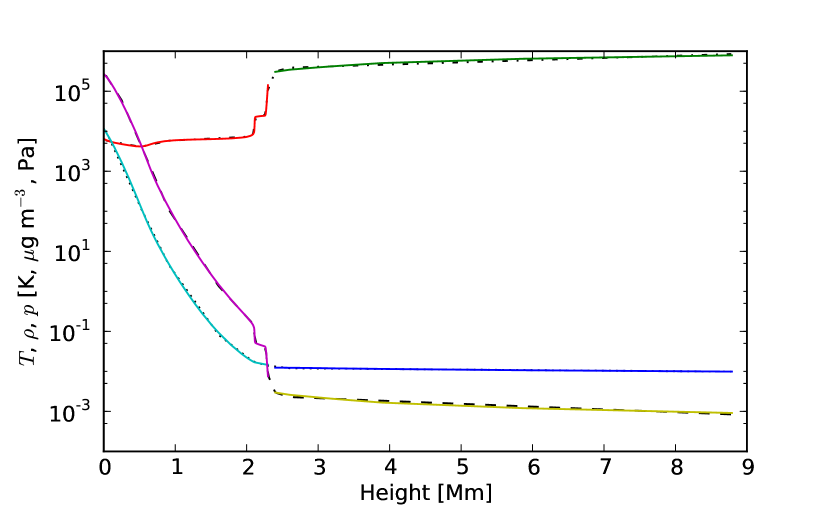
Figure 1: Interpolated 1D fits to vertical hydrostatic atmospheric profiles (Vernazza et al., 1981; McWhirter et al., 1975, former up to 2.3 Mm; latter above 2.4 Mm): thermal pressure $p$ [Pa] (dotted, light blue to blue), plasma density $\rho\,[\,\mu{\rm g}\,{\rm m^{-3}}]$ (dashed, purple to yellow) and temperature $T\,[\,{\rm K}]$ (dash-dotted, red to green).

In the reference data there are pronounced steps in temperature and density, corresponding to the transition region around $2.2\,{\rm Mm}$. The steady rise in temperature from the minimum $T\simeq 4200\,{\rm K}$ for $h\simeq 500\,{\rm km}$ reaches the critical temperature range $T>10^{4}\,{\rm K}$ over which full ionization of hydrogen occurs, followed subsequently by increases to the critical temperatures first for single and then double ionization of the helium to occur almost completely. To preserve the pressure equilibrium the density gradient must decrease and consequently the temperature gradient also accelerate in this region until the plasma is almost entirely ionized. Thereafter temperature and density resume more steady gradients. The pressure gradient, however, remains relatively smooth, preserving the hydrostatic equilibrium.

The pressure profiles described by Vernazza et al. (1981) and McWhirter et al. (1975) do not include any magnetic pressure , although a magnetic field is present and therefore the total pressure is in global magnetohydrostatic equilibrium. For our approach we require ambient conditions, in the absence of any magnetic forces, to be in hydrostatic equilibrium, which these profiles are not. We therefore need to construct such equilibrium vertical profiles from the reference data for density, pressure and temperature, which will recover the reference data profiles after we add the magnetic flux tube while preserving magnetohydrostatic equilibrium.

The vertical pressure balance in the absence of magnetic field may be expressed by

$$\frac{\,{\rm d}p{{}_{\rm v}}}{\,{\rm d}z}=\rho{{}_{\rm v}}g\Rightarrow\quad p{{}_{\rm v}}(z)=p_{\rm ref}({z_{\min}})+\int_{z_{\min}}^{z}\rho{{}_{\rm v}}(z^{*})g\,{\rm d}z^{*},$$ (1)

in which $p{{}_{\rm v}}$ and $\rho{{}_{\rm v}}$ represent the purely hydrothermal plasma pressure and density respectively. Coordinate $\hat{{{\mbox{\boldmath$z$}}}}$ is the projection along the solar radial direction $\hat{{{\mbox{\boldmath$R$}}}}$ and $z=0$ corresponds to $R=R_{\odot}$. The gravitational acceleration $g$ varies only slightly over the range of interest. Here it is assumed constant, $-274\,{\rm m\,s^{-2}}$, but $g$ varying with $z$ is also applicable. $p_{\rm ref}({z_{\min}})\simeq 10245\,{\rm Pa}$ is interpolated from Vernazza et al. (1981) at ${z_{\min}}=30\,{\rm km}$.

From the equation of state the temperature profile is

$$T{{}_{\rm v}}(z)=\frac{p{{}_{\rm v}}}{R_{\rm gas}\rho{{}_{\rm v}}},$$ (2)

with the gas constant $R_{\rm gas}$. The resulting pressure and temperature profiles are significiantly higher than the reference profiles. An ambient average magnetic field strength of up to $50\,{\rm mT}$ at the photosphere and $1\,{\rm mT}$ in the corona (Aschwanden, 2005, Ch. 1.8) account for the additional pressure. With the magnetic field and requisite corrections to plasma pressure, the reference profiles are recovered. To do so we also require modest enhancement of the reference density profile $\rho_{\rm ref}$ to obtain

$$\rho{{}_{\rm v}}=\rho_{\rm ref}(z)+\rho_{0}\exp\left(-\frac{z}{z_{\alpha}}\right),$$ (3)

with $\rho_{0}\simeq 0.01\,{\rm g}\,{\rm m^{-3}}$ and $z_{\alpha}\simeq 98\,{\rm km}$. This compares to $\rho_{\rm ref}(0)\simeq 0.27\,{\rm g}\,{\rm m^{-3}}$. So the hydrostatic atmosphere, absent any magnetic field, is specified by $p{{}_{\rm v}},\,\rho{{}_{\rm v}}$ and $T{{}_{\rm v}}$.

Here the particular choice of hydrothermal background is prescribed by the solar atmosphere. In general other backgrounds can be applied, subject to the requirement that the pressure gradient be parallel to the flux tube.

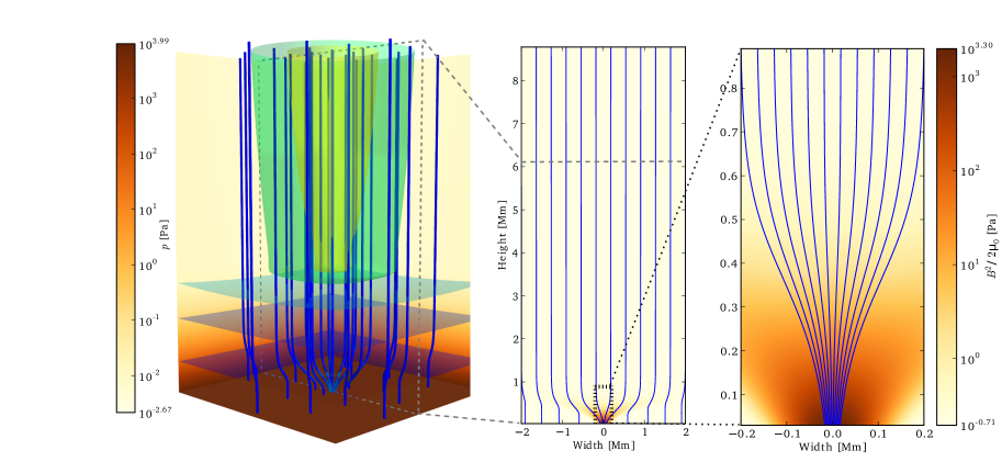
Figure 2: On the left a 3D rendition of the magnetic flux tube includes the magnetic field lines (reducing field strength, turquoise – blue). The rear and bottom surfaces display the thermal pressure (reducing, brown – yellow) and the isosurfaces depict the plasma-$\beta$ (purple – green $\simeq 277,1,0.08,0.025,0.016$). A vertical 2D-slice of the magnetohydrostatic background magnetic pressure is illustrated in the middle image. Some representative field lines are overplotted in blue. The box (black, dotted) encloses the region magnified for display in the image on the right.

2.2 Magnetic Field Construction

Embedded within this hydrostatic background we model a vertical open magnetic flux tube, representing one footpoint of a coronal loop. The other footpoint is presumed to be at a distance beyond the horizontal extent of our numerical domain. The arch of the loop occurs much higher in the corona than the vertical extent of our model, such that the flux tube may be regarded as vertically aligned. The region enclosing our model may reasonably be approximated either in cylindrical polar coordinates, with radius measured from the axis of the flux tube, or in Cartesian coordinates, with $x,y$ the local analogue of the longitudinal and latitudinal surface coordinates.

We elaborate the method of a self-similar expanding magnetic flux tube developed by Schlüter & Temesváry (1958) and applied variously for 2D (e.g. Deinzer, 1965; Low, 1980; Schüssler & Rempel, 2005; Gordovskyy & Jain, 2007; Fedun et al., 2011; Shelyag et al., 2011).

Alternative approaches may be considered, such as the thin flux tube approximation (e.g. Roberts & Webb, 1978). To first order the effects of magnetic tension and horizontal inhomgeneity on the global pressure balance may be neglected. In our model we anticipate these effects may be significant given the strong curvature of the magnetic field lines approaching the transtion region, and given how density inhomogeneity within each layer varies with height.

Another approach is to apply a potential field to the prescribed atmosphere and allow the system to relax numerically (e.g. Solanki & Steiner, 1990; Khomenko et al., 2008). Simulations of non-potential perturbations may then be applied to this equilibrium. For models utilising very large data arrays there may be considerable numerical overheads before the simulations can proceed. An advantage of our approach, is that the pressure balance is specified analytically, and altering the background atmosphere, perhaps to represent different regions of the solar atmosphere, or to investigate alternative field configurations does not require lengthy preliminary numerical calculations.

For a three-dimensional magnetic field describing the vertical flux tube and a weak ambient field, we define its components by the relations

$$B_{r}=-\frac{\partial f}{\partial z}{B_{0z}}{G}-r\frac{\partial{B_{bz}}}{\partial z},~{}~{}B_{\phi}=0,~{}~{}B_{z}=\frac{\partial f}{\partial r}{B_{0z}}{G}+2{B_{bz}},$$ (4)

in which ${B_{bz}}$ represents a vertically diminishing background term, and ${B_{0z}},\,f$ and ${G}$ prescribe the self-similar expanding axially symmetric magnetic flux tube. By construction $\nabla\cdot{{\mbox{\boldmath$B$}}}=0$ is preserved. Here $f$, ${B_{0z}}$, and ${B_{bz}}$ are defined by

$$f= {r}{B_{0z}}\quad\quad\quad\, [LB],$$ (5)

$${B_{0z}}= {b_{01}}\exp\left({-\frac{z}{{z_{1}}}}\right)+{b_{02}}\exp\left({-\frac{z}{{z_{2}}}}\right) [B],$$ (6)

$${B_{bz}}= {b_{00}}\exp\left(-\frac{z}{{z_{b}}}\right) [B],$$ (7)

where the dimensional units for each are shown in []. ${b_{01}}$, ${b_{02}}$ and ${b_{00}}$ are constants, controlling the strength of the vertical component of the magnetic field along and around the axis of the flux tube. ${z_{1}}$ and ${z_{2}}$ are included to scale the magnetic field strength along the axis with the plasma pressure above and below the transition region. The ratio of thermal (and kinetic) to magnetic pressure is denoted plasma-$\beta$. ${z_{b}}$ scales the ambient magnetic field with the pressure in the corona, thus ensuring plasma-$\beta<1$ outside the flux tube and maintaining thermal pressure greater than zero at large $z$.

We set the function ${B_{0z}}{G}$ to be the normalised gaussian with respect to $r$ over $0\leq r<\infty$. The inclusion of ${B_{0z}}$ in the coefficient of the gaussian is necessary to ensure the shape of the flux tube is consistent as it expands to balance the external pressure with increasing height.

$${G}= \frac{2{\ell}}{\sqrt{\pi}{f_{0}}}\exp\left[-\left(\frac{f}{{f_{0}}}\right)^{2}\right]\quad\quad\, [B^{-1}].$$ (8)

This arrangement ensures a purely vertical magnetic field along the axis of the flux tube and a diminishing field strength with increasing radius and height. The argument of the gaussian function must be dimensionless so the dimension of the horizontal scaling length ${f_{0}}$ is $[LB]$. For the definition of the magnetic field in Eq. (4) to be physically consistent ${G}$ must have dimension $[B^{-1}]$ and so ${\ell}$, an appropriate normalising length scale, is included in the coefficient.

Explicitly the components of the magnetic field for a flux tube centred around $r=0$ are

$$B_{r} =-f{G}\frac{\partial{B_{0z}}}{\partial z}-r\frac{\partial{B_{bz}}}{\partial z},$$ (9)

$$B_{z} ={{B_{0z}}^{2}{G}}+2{B_{bz}}.$$ (10)

A 3D view of the flux tube is represented in the left panel of Fig. 2 with representative magnetic field lines plotted against the backdrop of thermal pressure and through sample isosurfaces of the plasma-$\beta$. Projected from this is a vertical 2D-slice along the axis of magnetic pressure overplotted with such field lines. These diverge radially due to the negative pressure gradient below the transition region, but then are approximately vertical into the lower corona. For closer inspection a 2D-cut near the footpoint of the flux tube is magnified in the right-hand panel of Fig. 2.

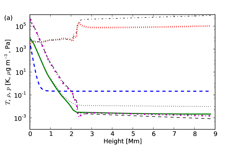
Figure 3: (a) 1D-slices along the model magnetic flux tube axis of $p\,[Pa]$ thermal (green, solid) and magnetic (blue, dashed) pressures, $\rho\,[\,\mu{\rm g}\,{\rm m^{-3}}]$ plasma density (purple, dash-dotted), and $T\,[\,{\rm K}]$ temperature (red, dotted) all superimposed on the referenced profiles (black) of Fig. 1. (b) The same 1D-slices as (a), but now at radius from the flux tube axis $r\simeq 2\sqrt{2}\,{\rm Mm}$.

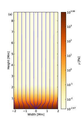
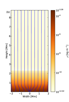
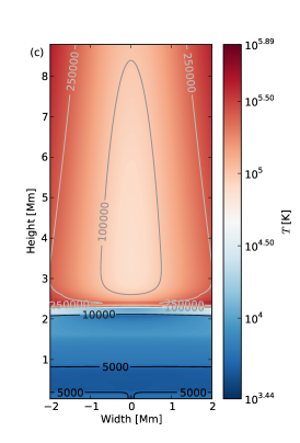
Figure 4: Vertical 2D-slice log profile of the magnetohydrostatic background (a) thermal pressure $p$, (b) density $\rho$ and (c) temperature $T$. Magnetic field lines (solid, blue) are overplotted in (a) and (b).

$f$ and ${G}$ may be expressed in Cartesian or cylindrical polar coordinates, without affecting the resulting relations for pressure. In Cartesian coordinates the components of the magnetic field may be recast as

$$B_{x} =\cos\phi B_{r}=-x\left(\frac{\partial{B_{bz}}}{\partial z}+{{B_{0z}}{G}}\frac{\partial{B_{0z}}}{\partial z}\right),$$ (11)

$$B_{y} =\sin\phi B_{r}=-y\left(\frac{\partial{B_{bz}}}{\partial z}+{{B_{0z}}{G}}\frac{\partial{B_{0z}}}{\partial z}\right),$$ (12)

$$B_{z} ={{B_{0z}}^{2}{G}}+2{B_{bz}}.$$ (13)

Note the complexity of the magnetic field construction in this example is again imposed by the structure of the lower atmosphere, incorporating the transition region. A magnetic flux tube structure with only one exponential may be adequate for modelling below the photosphere, or only in either the chromosphere or the corona. If plasma-$\beta>1$ outside the flux is not required, the terms including ${B_{bz}}$ may be neglected. Conversely a more complex construction may be considered. Providing the terms ${B_{0z}}$ and ${B_{bz}}$ have suitable dependence only on $z$, the approach for finding the magnetohydrostatic corrections to $p$ and $\rho$ described in this paper will apply. In this respect the model may have more general application.

2.3 Total pressure and density

For a background atmosphere supporting a magnetic flux tube in static equilibrium the total pressure $P$ must satisfy the equation of pressure balance:

$$\nabla P=\nabla p+\nabla\frac{|{{\mbox{\boldmath$B$}}}|^{2}}{2\mu_{0}}+({{\mbox{\boldmath$B$}}}\cdot\nabla){\color[rgb]{0,0,0}{\frac{{{\mbox{\boldmath$B$}}}}{\mu_{0}}}}=\rho{{\mbox{\boldmath$g$}}},$$ (14)

where the three inner terms are, respectively, the thermal/kinetic pressure gradient, the magnetic pressure gradient and the magnetic tension force. The latter is non-zero due to the curvature of the field lines. $\mu_{0}$ is the vacuum magnetic permeability coefficient.

Eq. (14) can be solved by integrating for each vector component (see Appendix B for details). First, it is convenient to separate the pressure and density into parts depending only on the hydrostatic pressure gradient $p_{{}_{\rm v}}$ and $\rho_{{}_{\rm v}}$, and the horizontal corrections in the global background pressure and density $p_{{}_{\rm h}}$ and $\rho_{{}_{\rm h}}$, required to restore the pressure balance arising from the presence of local magnetic pressure and tension forces due to the magnetic flux tube. Thus the total pressure gradient is

$${\color[rgb]{0,0,0}{\nabla P}}=\nabla p_{{}_{\rm v}}+\nabla p_{{}_{\rm h}}+\nabla\frac{|{{\mbox{\boldmath$B$}}}|^{2}}{2}+({{\mbox{\boldmath$B$}}}\cdot\nabla){{\mbox{\boldmath$B$}}}=(\rho_{h}+\rho_{v}){{\mbox{\boldmath$g$}}},$$ (15)

where for convenience, the unit of magnetic field is chosen such that $\mu_{0}=1$. $p_{{}_{\rm v}}$ and $\rho{{}_{\rm v}}$, specified by Eqs. (1) and (3) respectively, are constant on the horizontal plane and independent of magnetic effects, so can be excluded from the determination of the magnetohydrostatic terms.

The remaining terms in Eq. (15) are related independently of $p{{}_{\rm v}}$ and $\rho{{}_{\rm v}}$. The $r$-component,

$$\frac{\partial p_{{}_{\rm h}}}{\partial r}+\frac{\partial}{\partial r}\left(\frac{|{{\mbox{\boldmath$B$}}}|^{2}}{2}\right)+B_{r}\frac{\partial B_{r}}{\partial r}+B_{z}\frac{\partial B_{r}}{\partial z}=0,$$ (16)

can be integrated directly for the flux tube specified in Section 2.2 to obtain the thermal pressure $p{{}_{\rm h}}(r,z)$ as

$$p_{{}_{\rm h}}={\color[rgb]{0,0,0}{B^{\dagger}}},$$ (17)

in which $B^{\dagger}$ is an expression dependent on $r,z$ as detailed in Eq. (B.4) of Appendix B.

Integrating the $z$-component remaining from Eq. (15),

$$\frac{\partial p_{{}_{\rm h}}}{\partial z}+\frac{\partial}{\partial z}\left(\frac{|{{\mbox{\boldmath$B$}}}|^{2}}{2}\right)+B_{r}\frac{\partial B_{z}}{\partial r}+B_{z}\frac{\partial B_{z}}{\partial z}=\rho{{}_{\rm h}}g,$$ (18)

yields a solution of the form

$$p{{}_{\rm h}}={\color[rgb]{0,0,0}{B^{\dagger}}}+\int\rho{{}_{\rm h}}g+B^{*}\,{\rm d}z,$$ (19)

in which $B^{*}$ comprises the residual terms after subtracting $\partial B^{\dagger}/\partial z$ from under the integral. Eq. (19) must equal Eq. (17), requiring

$$\int\rho{{}_{\rm h}}g+B^{*}\,{\rm d}z=0.$$

This can be satisfied by setting $\rho{{}_{\rm h}}=-g^{-1}B^{*}$, for which $B^{*}$ is specified in Eq. (29) of Appendix B. The thermal pressure and the density are now fully specified by

$$p=p_{{}_{\rm v}}+p_{{}_{\rm h}},\quad\rho=\rho_{{}_{\rm v}}+\rho_{{}_{\rm h}}.$$

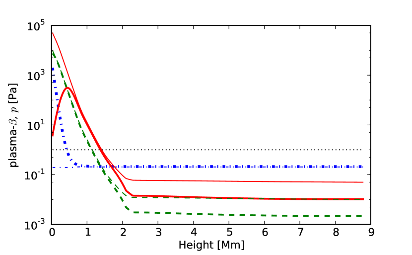
Figure 5: 1D-slices of thermal (green, dashed) and magnetic (blue, dash-dotted) pressures $p\,[Pa]$, and the plasma-$\beta$ (red, solid) along the magnetic flux tube axis (thick lines) and at axial radius $r\simeq 2\sqrt{2}\,{\rm Mm}$ (thin lines). The position of plasma-$\beta=1$ is included (black, dotted) for comparison.

The vertical profiles of the pressure, density and temperature thus derived are illustrated as 1D-slices in Fig. 3a along the axis of the magnetic flux tube and in Fig. 3b outside the flux tube (at radius $r=2\sqrt{2}\,{\rm Mm}$). The axis of the flux tube is slightly over-dense in the corona, and the temperature is consequently up to an order of magnitude lower than the reference data. At the edge of the model the density and temperature profiles tend to those of the hydrostatic background.

The vertical 2D-slices of the pressure, density and temperature are also displayed in Fig. 4. While a simulation might not extend to a radius exceeding $2\,{\rm Mm}$, it is included here to confirm that the flux tube remains physically valid beyond the numerical domain. The model has also been checked horizontally to $\pm 5\,{\rm Mm}$ and retains the features consistent with the reference data. The horizontal stratification is much weaker than the vertical, so is most apparent in Fig. 4c, because temperature exhibits less vertical stratification than plasma pressure or density. The flux tube plasma is cooler than the ambient plasma.

In Fig. 5 the variation in plasma-$\beta$ along the flux tube axis is plotted for the model magnetohydrostatic background along with the magnetic and thermal pressure profiles. Note, in the corona the magnetic pressure inside and outside the flux tube is similar, but plasma-$\beta\lesssim 0.01$ along the axis and plasma-$\beta\simeq 0.05$ outside differ significantly.

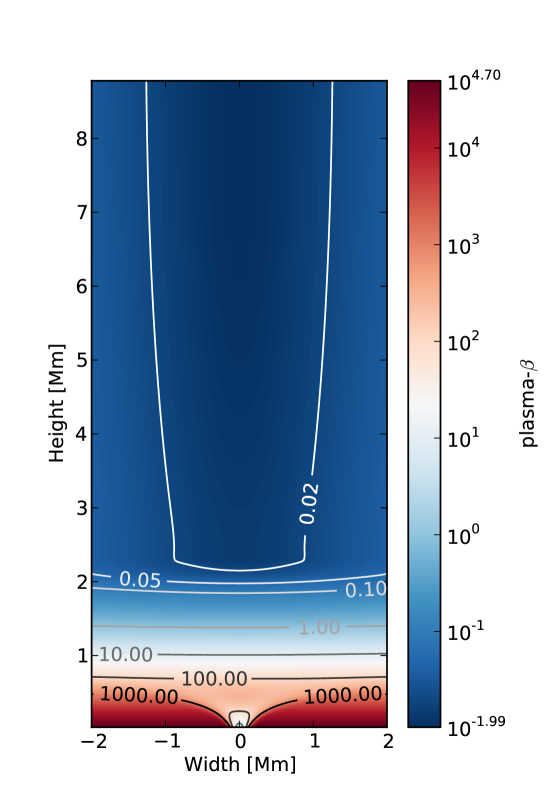
Figure 6: Vertical 2D-slice of the log magnetohydrostatic background plasma-$\beta$; the ratio of thermal to magnetic pressure.

The vertical 2D-slice of the log of plasma-$\beta$ is also depicted in Fig. 6. Note in both illustrations plasma-$\beta>1$ everywhere below $1.5\,{\rm Mm}$, indicating the dominance of thermal pressure, and $\beta<1$ everywhere above, indicating the dominance of magnetic pressure even below the transition region. There is a pronounced kink in the structure of the plasma-$\beta$ about $z=2.2\,{\rm Mm}$, corresponding to the step in plasma density and temperature at the transition region. Inclusion of these features may help to identify critical transport processes in simulations as propagating waves reach the transition region.

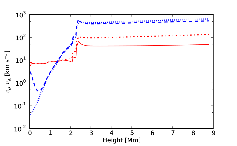
Figure 7: Vertical 1D-slices of the magnetohydrostatic background sound speed $c{{}_{\mathrm{s}}}$ (red) and the Alfvén speed $v_{\rm A}$ (blue). Profiles are plotted along the magnetic flux tube axis (solid, dashed) and at axial radius $r\simeq 2\sqrt{2}\,{\rm Mm}$ (dash-dotted, dotted).

The 1D-slices of the sound speed $c{{}_{\mathrm{s}}}$ and Alfvén speed $v_{\rm A}$ of the magnetohydrostatic background are displayed in Fig. 7. Inside and outside the magnetic flux tube $c{{}_{\mathrm{s}}}$ is similar below the transition region, but diverges significantly above. $v_{\rm A}$ inside and outside the flux tube is quite different below the temperature minimum at $z\simeq 500\,{\rm km}$ but then is similar after that. In the transition region the stepped gradients of $c{{}_{\mathrm{s}}}$ and $v_{\rm A}$ are very similar to each other, which may mean Alfvén waves could be subject to reflective effects analogous to those of sound waves.

2.4 Avoiding negative density and unphysical effects

For our model the axial footpoint strength is $100\,{\rm mT}\,(1000\,{\rm G})$ at the photosphere, yielding a full width half maximum (FWHM) of about $100\,{\rm km}$. This is illustrated in Fig. 8 for $z=3\,{\rm km}$ with a horizontal 1D-slice of the magnetic field strength (maximum $70\,{\rm mT}$) through the flux tube axis. The FWHM of $120\,{\rm km}$ at $z=3\,{\rm km}$ is indicated by vertical dotted lines and the half maximum by the horizontal dotted line. This is large enough to adequately resolve the profile with a practicable numerical resolution.

The chosen parameters in SI units as identified in this paper are ${b_{01}}\simeq 0.7\,{\rm mT}$, ${b_{02}}\simeq 0.01\,{\rm mT}$, ${f_{0}}\simeq 40\,{\rm mT}\,{\rm Mm}$, ${z_{1}}\simeq 0.17\,{\rm Mm}$, ${z_{2}}\simeq 175\,{\rm Mm}$, ${z_{b}}\simeq 5\cdot 10^{4}\,{\rm Mm}$ and ${b_{00}}\simeq 0.35\,{\rm mT}$. The scaling length ${\ell}\simeq 8\,{\rm Mm}$. These parameters must be chosen to adequately track the total pressure gradient, while generating a plasma-$\beta$ profile consistent with the physical model.

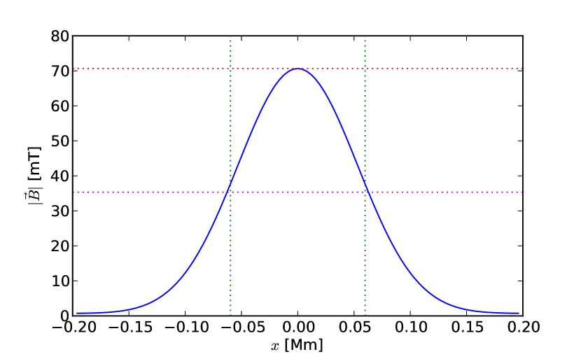
Figure 8: Horizontal 1D-slice of the magnetic field strength $|{{\mbox{\boldmath$B$}}}|$ (solid, blue) through the axis of the magnetic flux tube at $z=3\,{\rm km}$. Also indicated are the FWHM, $160\,{\rm km}$ (vertical, dotted) and the half maximum (magenta, dotted).

Our method requires an increase in plasma density inside the magnetic flux tube to balance the magnetic pressure and tension forces and so the temperature is lower than outside. The mean footpoint temperature (at $z=3\,{\rm km}$) within a radius of $50\,{\rm km}$ is $T\simeq 3600\,{\rm K}$. This is low compared to observational estimates nearer to $4000\,{\rm K}$, however the model is static, while in the solar atmosphere, turbulence may effect the observed temperatures and also influence the overall pressure balance.

It is important to recognise that $p_{{}_{\rm h}}$ and $\rho_{{}_{\rm h}}$ may take negative as well as positive values, subject to the constraints that the sums $p_{{}_{\rm v}}+p_{{}_{\rm h}}>0$, $\rho_{{}_{\rm v}}+\rho_{{}_{\rm h}}>0$ for any location in the domain. It is also important that they are sufficiently greater than zero, such that they remain positive and physically consistent even when the dynamical fluctuations are included during simulations. Note the thermal pressure gradient at the transition region exhibits some of the stepped structure evident in the temperature and density gradients, although the total pressure gradient is relatively smooth.

Within this transition region the plasma-$\beta$ falls substantially so that magnetic pressures predominate. This is where the density is low and rather sensitive to the strongest perturbations, so it is essential to ensure the background $\rho$ is adequate to contain any large negative perturbations.

3 Summary and Discussion

We have solved analytically the MHD pressure balance equation for a set of single open vertical magnetic flux tube configurations in magnetohydrostatic equilibrium within a realistic solar atmosphere, stratified in pressure, plasma density, temperature and magnetic field strength. The solutions are necessarily not inherently simplified, comprising a sum of multiple terms defining the pressure and plasma density functions, and include in this example ten parameters. They can, however, be easily coded and visualised. For high performance computing the functions can also be conveniently parallelized within numerical simulations.

The arrangement makes it possible to include the challenging stepped gradients in the transition region, rather than a smooth approximation to this profile. The free parameters in the model make it feasible to adjust the design for numerics in order to handle strong dynamical fluctuations without obtaining unphysical negativity for pressure or plasma density.

For mathematical transparency the flux tube is an idealised model, without torsion or any axial asymmetry, and the solar atmosphere is simplified to exclude local turbulence and fluctuations. However, we have endeavoured to embed the flux tube in a realistic gravitationally stratified background atmosphere, matching closely the better estimates available from theory and observation. Our model does not critically depend on the prescription of the ambient magnetic pressure gradient or the precise parametarization of the magnetic flux tube, so should data become available this would constrain the model more accurately, but would not invalidate it.

Exploring the magnetohydrostatic states of the model gives an indication for the physical constraints on magnetic field configuration, pressure, density and temperature, for which equilibrium is valid. It appears from this result, that the over-dense features of magnetic flux tubes in the solar corona, may be a natural prerequisite to balance the internal and external pressures. With this configuration a footpoint strength in excess of $100\,{\rm mT}$ or FWHM for this footpoint strength in excess of $100\,{\rm km}$ tend towards inducing regions of negative plasma density or pressure.

Our future work will include applying this analytic flux tube solution as the background for numerical studies of the energy transport mechanisms between the photosphere and the solar corona. We expect it to form the basis of a broad suite of such numerical models. It is worth explaining the derivation independently, which might otherwise be subsumed in a more general article also relating an array of numerical results. The aim of the present paper is to make the analytical result available for more general applications, further analysis and to promote the development of the model. The interactions between multiple flux tubes and alternative flux tube geometry might be considered, such as torsional or arched tubes.

Appendix A Dimensional quantities

Table 1: Dimensions of physical quantities used to non-dimensionalise the numerical equations.

Physics	Symbol	Dimension	Units
Length	$L$	$[L]$	$2\times 10^{3}$	$\,{\rm m}$
Velocity	$u$	$[u]$	$10^{3}$	$\,{\rm m}\,{\rm s}^{-1}$
Density	$\rho$	$[\rho]$	$10^{-6}$	$\,{\rm kg}\,{\rm m^{-3}}$
Time	$t$	$[L]/[u]$	$2$	$\,{\rm s}$
Temperature	$T$	$[T]$	$1$	$\,{\rm K}$
Energy Density	$e$	$[\rho][u]^{2}$	$1$	J$\,{\rm m^{-3}}$
Magnetic Field	$B$	$\sqrt{\mu_{0}}[\rho]^{\frac{1}{2}}[u]$	$1.12..\times 10^{-3}$	T †
Pressure	$p$	$[\rho][u]^{2}$	$1$	Pa

${}^{\dagger}\,\mu_{0}=4\pi\times 10^{-7}$ N A^-2

These equations can be non-dimensionalised by dividing the variables with typical units, as detailed in Table 1.

Appendix B Solution to background static equilibrium

In this Appendix we explicitly outline the solution to Eqs. (16) and (18).

B.1 Basic quantities and derivatives

Listed here are the form of the magnetic field components and the various derivatives of the expressions which will be required in the calculations.

$${\color[rgb]{0,0,0}{B_{r}=-f{G}\frac{\partial{B_{0z}}}{\partial z}-r\frac{\partial{B_{bz}}}{\partial z},\quad B_{z}={{B_{0z}}^{2}{G}}+2{B_{bz}}}},$$

$$\frac{\partial f}{\partial r}={{B_{0z}}}{},\quad\frac{\partial f}{\partial z}={r}{}\frac{\partial{B_{0z}}}{\partial z},\quad\frac{\partial{G}}{\partial f}=-\frac{2f{G}}{{f_{0}}^{2}},\quad$$

$$\frac{\partial{G}}{\partial r}=\frac{\partial{G}}{\partial f}\frac{\partial f}{\partial r}=-\frac{2{B_{0z}}f{G}}{{f_{0}}^{2}},\quad\frac{\partial{G}}{\partial z}=-\frac{2f{G}r}{{f_{0}}^{2}}\frac{\partial{B_{0z}}}{\partial z}.$$

B.2 Magnetic pressure terms

The magnetic pressure terms will integrate directly in Eq. (14) and so we shall not require the derivatives. They are noted here for inclusion in the final result.

$$\frac{|{{\mbox{\boldmath$B$}}}|^{2}}{2} = \frac{B_{r}^{2}}{2}+\frac{B_{z}^{2}}{2}$$

$$= {\color[rgb]{0,0,0}{\frac{1}{2}\left({f{G}}\frac{\partial{B_{0z}}}{\partial z}+r\frac{\partial{B_{bz}}}{\partial z}\right)^{2}+\frac{1}{2}\left({{B_{0z}}^{2}{G}}+2{B_{bz}}\right)^{2}}}.$$

B.3 Magnetic tension force

The components of the magnetic tension force are given by the general expressions by components $\hat{{{\mbox{\boldmath$r$}}}}$ and $\hat{{{\mbox{\boldmath$z$}}}}$, respectively,

$$B_{r}\frac{\partial B_{r}}{\partial r}+B_{z}\frac{\partial B_{r}}{\partial z},$$ (20)

$$B_{r}\frac{\partial B_{z}}{\partial r}+B_{z}\frac{\partial B_{z}}{\partial z}.$$ (21)

We will require the derivatives in these expressions as follows:

$$\frac{\partial B_{r}}{\partial r} = -\left({{B_{0z}}{G}}+{f}\frac{\partial{G}}{\partial r}\right)\frac{\partial{B_{0z}}}{\partial z}-\frac{\partial{B_{bz}}}{\partial z}$$ (22)

$$= {{B_{0z}}{G}}\left(\frac{2f^{2}}{{f_{0}}^{2}}-1\right)\frac{\partial{B_{0z}}}{\partial z}-\frac{\partial{B_{bz}}}{\partial z}$$

$$\frac{\partial B_{r}}{\partial z} = -\left({{G}}\frac{\partial f}{\partial z}+{f}\frac{\partial{G}}{\partial z}\right)\frac{\partial{B_{0z}}}{\partial z}$$

$$-f{G}\frac{\partial}{\partial z}\left(\frac{\partial{B_{0z}}}{\partial z}\right)-r\frac{\partial^{2}{B_{bz}}}{\partial z^{2}}$$

$$= {{G}r}\left(\frac{2f^{2}}{{f_{0}}^{2}}-1\right)\frac{\partial{B_{0z}}}{\partial z}^{2}-f{G}\frac{\partial^{2}{B_{0z}}}{\partial z^{2}}-r\frac{\partial^{2}{B_{bz}}}{\partial z^{2}}$$

$$\frac{\partial B_{z}}{\partial r} = {{B_{0z}}^{2}}\frac{\partial{G}}{\partial r}=-\frac{2{B_{0z}}^{3}f{G}}{{f_{0}}^{2}},$$ (24)

$$\frac{\partial B_{z}}{\partial z} = {2{B_{0z}}{G}}\frac{\partial{B_{0z}}}{\partial z}+{{B_{0z}}^{2}}\frac{\partial{G}}{\partial z}+2\frac{\partial{B_{bz}}}{\partial z}$$ (25)

$$= {2{B_{0z}}{G}}\left(1-\frac{f^{2}}{{f_{0}}^{2}}\right)\frac{\partial{B_{0z}}}{\partial z}+2\frac{\partial{B_{bz}}}{\partial z}$$

B.4 Thermal pressure balancing magnetic field

Having prescribed the magnetic field we now seek to satisfy the pressure balance, first by solving Eq. (16) for the $r$-components. The first term of the right-hand side below is magnetic pressure. Subsequent terms yield the expression Eq. (20) by multiplying $B_{r}$ with (22) and $B_{z}$ with (B.3).

$$\frac{\partial p_{{}_{\rm h}}}{\partial r} = -\frac{\partial}{\partial r}\left(\frac{|{{\mbox{\boldmath$B$}}}|^{2}}{2}\right)+\cancel{{f{G}}\cdot{{B_{0z}}{G}}\left(\frac{2f^{2}}{{f_{0}}^{2}}-1\right)\frac{\partial{B_{0z}}}{\partial z}^{2}}$$

$$-f{G}\frac{\partial{B_{0z}}}{\partial z}\cdot\frac{\partial{B_{bz}}}{\partial z}+r\frac{\partial{B_{bz}}}{\partial z}\cdot{{B_{0z}}{G}}\left(\frac{2f^{2}}{{f_{0}}^{2}}-1\right)\frac{\partial{B_{0z}}}{\partial z}$$

$$-{r\frac{\partial{B_{bz}}}{\partial z}\cdot\frac{\partial{B_{bz}}}{\partial z}}-\cancel{{B_{0z}}^{2}{G}\cdot{{G}r}\left(\frac{2f^{2}}{{f_{0}}^{2}}-1\right)\frac{\partial{B_{0z}}}{\partial z}^{2}}$$

$$+{B_{0z}}^{2}{G}\cdot f{G}\frac{\partial^{2}{B_{0z}}}{\partial z^{2}}-2{B_{bz}}\cdot{{G}r}\left(\frac{2f^{2}}{{f_{0}}^{2}}-1\right)\frac{\partial{B_{0z}}}{\partial z}^{2}$$

$$+{B_{0z}}^{2}{G}\cdot r\frac{\partial^{2}{B_{bz}}}{\partial z^{2}}+{2{B_{bz}}\cdot r\frac{\partial^{2}{B_{bz}}}{\partial z^{2}}}+2{B_{bz}}\cdot f{G}\frac{\partial^{2}{B_{0z}}}{\partial z^{2}}$$

$$\ldots = -\frac{\partial}{\partial r}\left(\frac{|{{\mbox{\boldmath$B$}}}|^{2}}{2}\right)+\frac{\partial}{\partial r}\left(\frac{2{B_{bz}}f^{2}{G}}{{B_{0z}}^{2}}+\frac{{B_{bz}}{f_{0}}^{2}{G}}{{B_{0z}}^{2}}\right)\frac{\partial{B_{0z}}}{\partial z}^{2}$$

$$-\frac{{B_{bz}}{f_{0}}^{2}}{{B_{0z}}}\frac{\partial{G}}{\partial r}\frac{\partial^{2}{B_{0z}}}{\partial z^{2}}-\frac{{B_{0z}}{f_{0}}^{2}}{4}\frac{\partial{G}^{2}}{\partial r}\frac{\partial^{2}{B_{0z}}}{\partial z^{2}}$$

$$-\frac{\partial}{\partial r}\left(\frac{f^{2}{G}}{{B_{0z}}}+\cancel{\frac{{f_{0}}^{2}{G}}{2{B_{0z}}}}\right)\frac{\partial{B_{bz}}}{\partial z}\frac{\partial{B_{0z}}}{\partial z}+2r{B_{bz}}\frac{\partial^{2}{B_{bz}}}{\partial z^{2}}$$

$$+\cancel{\frac{{f_{0}}^{2}}{2{B_{0z}}}\frac{\partial{G}}{\partial r}\frac{\partial{B_{bz}}}{\partial z}\frac{\partial{B_{0z}}}{\partial z}}-\frac{{f_{0}}^{2}}{2}\frac{\partial{G}}{\partial r}\frac{\partial^{2}{B_{bz}}}{\partial z^{2}}-r\frac{\partial{B_{bz}}}{\partial z}^{2}$$

$$p_{{}_{\rm h}} = -\frac{|{{\mbox{\boldmath$B$}}}|^{2}}{2}+\left({\frac{2{B_{bz}}f^{2}{G}}{{B_{0z}}^{2}}}+{\frac{{B_{bz}}{f_{0}}^{2}{G}}{{B_{0z}}^{2}}}\right)\frac{\partial{B_{0z}}}{\partial z}^{2}$$

$$-\frac{{B_{bz}}{f_{0}}^{2}{G}}{{B_{0z}}}\frac{\partial^{2}{B_{0z}}}{\partial z^{2}}-\frac{{B_{0z}}{f_{0}}^{2}{G}^{2}}{4}\frac{\partial^{2}{B_{0z}}}{\partial z^{2}}-\frac{r^{2}}{2}\frac{\partial{B_{bz}}}{\partial z}^{2}$$

$$-\frac{f^{2}{G}}{{B_{0z}}}\frac{\partial{B_{bz}}}{\partial z}\frac{\partial{B_{0z}}}{\partial z}-\frac{{f_{0}}^{2}{G}}{2}\frac{\partial^{2}{B_{bz}}}{\partial z^{2}}+r^{2}{B_{bz}}\frac{\partial^{2}{B_{bz}}}{\partial z^{2}}.$$

The solution is constrained by $p=p{{}_{\rm v}}+p{{}_{\rm h}}$ such that any constant of integration, a function of $z$, may be expressed within $p{{}_{\rm v}}$. Note that this solution can be simplified if our model can neglect the ambient magnetic field ${B_{bz}}$, which outside the flux tube would result in plasma-$\beta>1$ in the corona and the chromosphere. Then

$$p_{{}_{\rm h}}=-\frac{|{{\mbox{\boldmath$B$}}}|^{2}}{2}-\frac{{B_{0z}}{f_{0}}^{2}{G}^{2}}{4}\frac{\partial^{2}{B_{0z}}}{\partial z^{2}}$$ (27)

B.5 Plasma density balancing magnetic field

To determine $\rho{{}_{\rm h}}$ it is also necessary to integrate $\partial p_{{}_{\rm h}}/\partial z$ in Eq. (18). For the magnetic tension terms of Eq. (21), $B_{r}$ is multiplied with the expression (24) and $B_{z}$ with (25).

$$\frac{\partial p_{{}_{\rm h}}}{\partial z} = \rho_{{}_{\rm h}}g-\frac{\partial}{\partial z}\left(\frac{|{{\mbox{\boldmath$B$}}}|^{2}}{2}\right)-r\frac{\partial{B_{bz}}}{\partial z}\cdot\frac{2{B_{0z}}^{3}f{G}}{{f_{0}}^{2}}$$

$$-\cancel{f{G}\frac{\partial{B_{0z}}}{\partial z}\cdot\frac{2{B_{0z}}^{3}f{G}}{{f_{0}}^{2}}}-{B_{0z}}^{2}{G}\cdot{\color[rgb]{0,0,0}{2\frac{\partial{B_{bz}}}{\partial z}}}$$

$$-{B_{0z}}^{2}{G}\cdot 2{B_{0z}}{G}\left(1-\cancel{\frac{f^{2}}{{f_{0}}^{2}}}\right)\frac{\partial{B_{0z}}}{\partial z}$$

$$-{\color[rgb]{0,0,0}{2{B_{bz}}\cdot 2{B_{0z}}{G}\left(1-\frac{f^{2}}{{f_{0}}^{2}}\right)\frac{\partial{B_{0z}}}{\partial z}+2{B_{bz}}\cdot 2\frac{\partial{B_{bz}}}{\partial z}}}$$

The solution to this must match that of Eq. (B.4). The match can be more easily identified if we add to this the following list of terms, each equating to zero:

$$+\frac{\partial}{\partial z}\left({2{G}r^{2}}{B_{bz}}\frac{\partial{B_{0z}}}{\partial z}^{2}\right)-\cancel{2}{{G}r^{2}\frac{\partial{B_{bz}}}{\partial z}\frac{\partial{B_{0z}}}{\partial z}^{2}}-{4{G}r^{2}}{B_{bz}}\frac{\partial{B_{0z}}}{\partial z}\frac{\partial^{2}{B_{0z}}}{\partial z^{2}}$$

$$+\frac{4f{G}r^{3}}{{f_{0}}^{2}}{B_{bz}}\frac{\partial{B_{0z}}}{\partial z}^{3},$$

$$+\frac{\partial}{\partial z}\left(\frac{{B_{bz}}{f_{0}}^{2}{G}}{{B_{0z}}^{2}}\frac{\partial{B_{0z}}}{\partial z}^{2}\right)+\frac{2{B_{bz}}{G}r^{2}}{{B_{0z}}}\frac{\partial{B_{0z}}}{\partial z}^{3}-\frac{2{B_{bz}}{f_{0}}^{2}{G}}{{B_{0z}}^{2}}\frac{\partial{B_{0z}}}{\partial z}\frac{\partial^{2}{B_{0z}}}{\partial z^{2}}$$

$$-{\frac{{f_{0}}^{2}{G}}{{B_{0z}}^{2}}\frac{\partial{B_{bz}}}{\partial z}\frac{\partial{B_{0z}}}{\partial z}^{2}}+\frac{2{B_{bz}}{f_{0}}^{2}{G}}{{B_{0z}}^{3}}\frac{\partial{B_{0z}}}{\partial z}^{3},$$

$$-\frac{\partial}{\partial z}\left(\frac{{B_{0z}}{f_{0}}^{2}{G}^{2}}{4}\frac{\partial^{2}{B_{0z}}}{\partial z^{2}}\right)+\left(\frac{{f_{0}}^{2}{G}^{2}}{4}-f^{2}{G}^{2}\right)\frac{\partial{B_{0z}}}{\partial z}\frac{\partial^{2}{B_{0z}}}{\partial z^{2}}$$

$$+\frac{{B_{0z}}{f_{0}}^{2}{G}^{2}}{4}\frac{\partial^{3}{B_{0z}}}{\partial z^{3}},$$

$$-\frac{\partial}{\partial z}\left(\frac{{B_{bz}}{f_{0}}^{2}{G}}{{B_{0z}}}\frac{\partial^{2}{B_{0z}}}{\partial z^{2}}\right)-\left({\frac{{f_{0}}^{2}{G}}{{B_{0z}}^{2}}}+{{2{G}r^{2}}}\right){B_{bz}}\frac{\partial{B_{0z}}}{\partial z}\frac{\partial^{2}{B_{0z}}}{\partial z^{2}}$$

$$+{{\frac{{B_{bz}}{f_{0}}^{2}{G}}{{B_{0z}}}}\frac{\partial^{3}{B_{0z}}}{\partial z^{3}}}+{\frac{{f_{0}}^{2}{G}}{{B_{0z}}}\frac{\partial{B_{bz}}}{\partial z}\frac{\partial^{2}{B_{0z}}}{\partial z^{2}}},$$

$$-\frac{\partial}{\partial z}\left({f{G}r}{}\frac{\partial{B_{bz}}}{\partial z}\frac{\partial{B_{0z}}}{\partial z}\right)+{f{G}r}{}\frac{\partial{B_{bz}}}{\partial z}\frac{\partial^{2}{B_{0z}}}{\partial z^{2}}+\bcancel{{f{G}r}{}\frac{\partial^{2}{B_{bz}}}{\partial z^{2}}\frac{\partial{B_{0z}}}{\partial z}}$$

$$+\left(\cancel{{{G}r^{2}}{}}-\frac{2f^{2}{G}r^{2}}{{f_{0}}^{2}}\right)\frac{\partial{B_{bz}}}{\partial z}\frac{\partial{B_{0z}}}{\partial z}^{2},$$

$$-\frac{\partial}{\partial z}\left(\frac{{f_{0}}^{2}{G}}{2}\frac{\partial^{2}{B_{bz}}}{\partial z^{2}}\right)+\frac{{f_{0}}^{2}{G}}{2}\frac{\partial^{3}{B_{bz}}}{\partial z^{3}}-\bcancel{{f{G}r}{}\frac{\partial^{2}{B_{bz}}}{\partial z^{2}}\frac{\partial{B_{0z}}}{\partial z}},$$

$$+\frac{\partial}{\partial z}\left({B_{bz}}r^{2}\frac{\partial^{2}{B_{bz}}}{\partial z^{2}}-\frac{r^{2}}{2}\frac{\partial{B_{bz}}}{\partial z}^{2}\right)+{B_{bz}}r^{2}\frac{\partial^{3}{B_{bz}}}{\partial z^{3}}.$$

If we filter out all of the derivative expressions, which can be integrated directly to return the same result as Eq. (B.4) any residual terms must disappear and hence we require

$$\int\,{\rm d}z\rho_{{}_{\rm h}}g - \left[\frac{2{B_{0z}}^{4}{G}r^{2}}{{f_{0}}^{2}}+{2{B_{0z}}^{2}{G}}-4{B_{bz}}\right]\frac{\partial{B_{bz}}}{\partial z}$$ (29)

$$+ \frac{{f_{0}}^{2}{G}}{2}\frac{\partial^{3}{B_{bz}}}{\partial z^{3}}+{B_{bz}}r^{2}\frac{\partial^{3}{B_{bz}}}{\partial z^{3}}-2{B_{0z}}^{3}{G}^{2}\frac{\partial{B_{0z}}}{\partial z}$$

$$- {{4{B_{bz}}{B_{0z}}{G}}}\left[1-\frac{f^{2}}{{f_{0}}^{2}}\right]\frac{\partial{B_{0z}}}{\partial z}+\frac{{f_{0}}^{2}{G}}{{B_{0z}}}\frac{\partial{B_{bz}}}{\partial z}\frac{\partial^{2}{B_{0z}}}{\partial z^{2}}$$

$$+ {f{G}r}{}\frac{\partial{B_{bz}}}{\partial z}\frac{\partial^{2}{B_{0z}}}{\partial z^{2}}-\frac{3{B_{bz}}{f_{0}}^{2}{G}}{{B_{0z}}^{2}}\frac{\partial{B_{0z}}}{\partial z}\frac{\partial^{2}{B_{0z}}}{\partial z^{2}}$$

$$+ \left[\frac{{f_{0}}^{2}{G}^{2}}{4}-{f^{2}{G}^{2}}-6{B_{bz}}{G}r^{2}\right]\frac{\partial{B_{0z}}}{\partial z}\frac{\partial^{2}{B_{0z}}}{\partial z^{2}}$$

$$- \left[\frac{2f^{2}{G}r^{2}}{{f_{0}}^{2}}+\frac{{f_{0}}^{2}{G}}{{B_{0z}}^{2}}+{{G}r^{2}}\right]\frac{\partial{B_{bz}}}{\partial z}\frac{\partial{B_{0z}}}{\partial z}^{2}$$

$$+ {B_{bz}}{G}\left[\frac{r^{2}}{{B_{0z}}}+\frac{2{f_{0}}^{2}}{{B_{0z}}^{3}}+\frac{4fr^{3}}{{f_{0}}^{2}}\right]\frac{\partial{B_{0z}}}{\partial z}^{3}$$

$$+ \frac{{B_{0z}}{f_{0}}^{2}{G}^{2}}{4}\frac{\partial^{3}{B_{0z}}}{\partial z^{3}}+\frac{{B_{bz}}{f_{0}}^{2}{G}}{{B_{0z}}}\frac{\partial^{3}{B_{0z}}}{\partial z^{3}}=0.$$

B.6 Divergence and pressure balance precision

In cylindrical polar coordinates the divergence of the magnetic field is given by

$$\nabla\cdot{{\mbox{\boldmath$B$}}} = \frac{1}{r}\frac{\partial}{\partial r}(rB_{r})+\cancel{\frac{1}{r}\frac{\partial B_{\phi}}{\partial\phi}}+\frac{\partial B_{z}}{\partial z}$$

$$= -\frac{1}{r}\left[\frac{\partial f}{\partial z}{B_{0z}}{G}+r\frac{\partial^{2}f}{\partial r\partial z}{B_{0z}}{G}+r\frac{\partial f}{\partial z}{B_{0z}}\frac{\partial{G}}{\partial f}\frac{\partial f}{\partial r}\right]$$

$$+ \frac{\partial f}{\partial r}\frac{\partial{B_{0z}}}{\partial z}{G}+\frac{\partial^{2}f}{\partial r\partial z}{B_{0z}}{G}+\frac{\partial f}{\partial r}{B_{0z}}\frac{\partial{G}}{\partial f}\frac{\partial f}{\partial z}$$

$$- \frac{1}{r}2r\frac{\partial{B_{bz}}}{z}+2\frac{\partial{B_{bz}}}{z}=0.$$

The resulting magnetic field configuration has been checked numerically with a mesh resolution $\delta x=10\,{\rm km}$ to verify

$$\nabla\cdot{{\mbox{\boldmath$B$}}}=\frac{\partial B_{x}}{\partial x}+\frac{\partial B_{y}}{\partial y}+\frac{\partial B_{z}}{\partial z}=0.$$

The resulting error scaled by the local strength of the field has mean of order $10^{-7}$, with peak of order $10^{-4}$.

The horizontal pressure balance

$$\frac{\partial p}{\partial x}+\frac{\partial}{\partial x}\frac{|{{\mbox{\boldmath$B$}}}|^{2}}{2}+B_{x}\frac{\partial B_{x}}{\partial x}+B_{y}\frac{\partial B_{x}}{\partial y}+B_{z}\frac{\partial B_{x}}{\partial z}=0$$

and vertical pressure balance

$$\frac{\partial p}{\partial z}+\frac{\partial}{\partial z}\frac{|{{\mbox{\boldmath$B$}}}|^{2}}{2}+B_{x}\frac{\partial B_{z}}{\partial x}+B_{y}\frac{\partial B_{z}}{\partial y}+B_{z}\frac{\partial B_{z}}{\partial z}-\rho g=0$$

have been verified numerically with $\delta x=10\,{\rm km}$ for the derived thermal pressure, density and specified magnetic field configuration. For the horizontal pressure balance $\epsilon<10^{-13}$ and for the vertical mean relative error $\epsilon\simeq 10^{-7}$ with peak of order $10^{-4}$. As $\delta x\rightarrow 0$ the relative error $\epsilon\rightarrow 0$.

For these and we use the same derivative scheme as applied in the Versatile Advection Code (Tóth, 1996) and the Sheffield Advanced Code for MHD (Shelyag et al., 2008), which we plan to employ for future simulations.

References

• Aschwanden (2005) Aschwanden M. J., 2005, Physics of the Solar Corona. An Introduction with Problems and Solutions (2nd edition)
• Aschwanden et al. (2001) Aschwanden M. J., Schrijver C. J., Alexander D., 2001, ApJ, 550, 1036
• Deinzer (1965) Deinzer W., 1965, ApJ, 141, 548
• Fedun et al. (2009) Fedun V., Erdélyi R., Shelyag S., 2009, SoPh, 258, 219
• Fedun et al. (2011) Fedun V., Shelyag S., Erdélyi R., 2011, ApJ, 727, 17
• Gascoyne & Jain (2009) Gascoyne A., Jain R., 2009, A&A, 501, 1131
• Gibson & Low (1998) Gibson S. E., Low B. C., 1998, ApJ, 493, 460
• Gordovskyy & Jain (2007) Gordovskyy M., Jain R., 2007, ApJ, 661, 586
• Hunter (2007) Hunter J. D., 2007, Computing In Science & Engineering, 9, 90
• Jones et al. (2001) Jones E., Oliphant T., Peterson P., Others, 2001, SciPy: Open source scientific tools for Python
• Khomenko et al. (2008) Khomenko E., Collados M., Felipe T., 2008, SoPh, 251, 589
• Low (1980) Low B. C., 1980, SoPh, 67, 57
• Manchester et al. (2004) Manchester W. B., Gombosi T. I., Roussev I., de Zeeuw D. L., Sokolov I. V., Powell K. G., Tóth G., Opher M., 2004, Journal of Geophysical Research (Space Physics), 109, 1102
• McWhirter et al. (1975) McWhirter R. W. P., Thonemann P. C., Wilson R., 1975, A&A, 40, 63
• Priest (1987) Priest E. R., 1987, Solar magneto-hydrodynamics.
• Ramachandran & Varoquaux (2011) Ramachandran P., Varoquaux G., 2011, Computing in Science & Engineering, 13, 40
• Roberts & Webb (1978) Roberts B., Webb A. R., 1978, SoPh, 56, 5
• Schlüter & Temesváry (1958) Schlüter A., Temesváry S., 1958, in Lehnert B., ed., Electromagnetic Phenomena in Cosmical Physics Vol. 6 of IAU Symposium, The Internal Constitution of Sunspots. p. 263
• Schüssler & Rempel (2005) Schüssler M., Rempel M., 2005, A&A, 441, 337
• Shelyag et al. (2008) Shelyag S., Fedun V., Erdélyi R., 2008, A&A, 486, 655
• Shelyag et al. (2011) Shelyag S., Fedun V., Keenan F. P., Erdélyi R., Mathioudakis M., 2011, Annales Geophysicae, 29, 883
• Shelyag et al. (2009) Shelyag S., Zharkov S., Fedun V., Erdélyi R., Thompson M. J., 2009, A&A, 501, 735
• Solanki & Steiner (1990) Solanki S. K., Steiner O., 1990, A&A, 234, 519
• Tóth (1996) Tóth G., 1996, Astrophys. Lett. & Commun., 34, 245
• Vernazza et al. (1981) Vernazza J. E., Avrett E. H., Loeser R., 1981, ApJS, 45, 635
• Vigeesh et al. (2012) Vigeesh G., Fedun V., Hasan S. S., Erdélyi R., 2012, ApJ, 755, 18
• Winebarger et al. (2003) Winebarger A. R., Warren H. P., Mariska J. T., 2003, ApJ, 587, 439
• Zwaan (1978) Zwaan C., 1978, SoPh, 60, 213