On Weingarten transformations of hyperbolic nets

Abstract.

Weingarten transformations which, by definition, preserve the asymptotic lines on smooth surfaces have been studied extensively in classical differential geometry and also play an important role in connection with the modern geometric theory of integrable systems. Their natural discrete analogues have been investigated in great detail in the area of (integrable) discrete differential geometry and can be traced back at least to the early 1950s. Here, we propose a canonical analogue of (discrete) Weingarten transformations for hyperbolic nets, that is, $C^{1}$-surfaces which constitute hybrids of smooth and discrete surfaces “parametrized” in terms of asymptotic coordinates. We prove the existence of Weingarten pairs and analyse their geometric and algebraic properties.

1. Introduction

The subject of the present paper is the determination and analysis of a canoncial class of transformations associated with so-called hyperbolic nets. The latter have been introduced recently in [HVR13] and constitute a discretization of surfaces in 3-space that are parametrized along asymptotic lines. A parametrization of a surface is called an asymptotic line parametrization if, at each point of the surface, parameter lines follow the distinguished directions of vanishing normal curvature. For smooth surfaces, one has unique asymptotic line parametrizations (up to reparametrization of parameter lines) around hyperbolic points, that is, around points of negative Gaussian curvature [Eis60]. It is natural to discretize parametrized surfaces by quadrilateral nets, also called quadrilateral meshes. Compared with, e.g., discrete triangulated surfaces, quadrilateral nets do not only discretize continuous surfaces understood as topological objects (point sets), but also reflect the combinatorial structure of parameter lines. While unspecified quadrilateral nets discretize arbitrary parametrizations, the discretization of distinguished types of parametrizations yields quadrilateral nets with special geometric properties. One of the most fundamental examples is the discretization of conjugate parametrizations by quadrilateral nets with planar faces. Discretizing more specific conjugate parametrizations then yields planar quadrilateral nets with additional properties. However, as asymptotic line parametrizations are not conjugate parametrizations, they are not modelled by quadrilateral nets with planar faces. Instead, asymptotic line parametrizations are properly discretized by quadrilateral nets with planar vertex stars, that is, nets for which every vertex is coplanar with its nearest neighbours. We use the terminology of [BS08], calling discrete nets with planar quadrilaterals Q-nets and (skew) quadrilateral nets with planar vertex stars A-nets. Q-nets and A-nets as discretizations of conjugate and asymptotic line parametrizations were already introduced in [Sau37].

Various aspects of continuous asymptotic line parametrizations have been discretized using A-nets. For example, the discretization of surfaces of constant negative Gaussian curvature as special A-nets, nowadays often called K-surfaces, can be found in [Sau50, Wun51]. In the context of the connections between geometry and integrability, the relation between discrete K-surfaces and Hirota’s [Hir77] algebraic discretization of the sine-Gordon equation was established much later [BP96]. For a special instance of this relation, see, for example, [Hof99] on discrete Amsler-surfaces. Discrete indefinite affine spheres [BS99b] are an example for the discretization of a certain class of smooth A-nets within affine differential geometry. The discrete Lelieuvre representation of A-nets and the related discrete Moutard equations are, for instance, treated in [NS97, BS99a, KP00, Dol01, DNS01, Nie02].

Based on the discretization of asymptotic line parametrizations by A-nets, hyperbolic nets arise as an extension of A-nets in the sense that elementary quadrilaterals of A-nets become extended to hyperbolic surface patches. More precisely, a hyperbolic net is a piecewise smooth surface composed of hyperboloid patches, where the latter refers to surface patches that are taken from doubly ruled quadrics, i.e., one-sheeted hyperboloids and hyperbolic paraboloids, by “cutting along asymptotic lines”. In order to obtain a hyperbolic net, hyperboloid patches are inserted into the skew quadrilaterals of a supporting discrete A-surface such that the tangent planes of edge-adjacent patches coincide along the common boundary edge (cf. Fig. 1). Hence, hyperbolic nets are $C^{1}$-surfaces which may be regarded as “hybrids” of smooth surfaces parametrized in terms of asymptotic coordinates and their discrete counterparts.

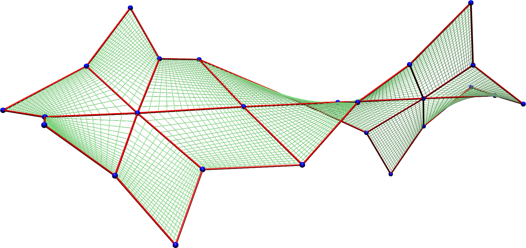
Figure 1. A hyperbolic net. The red segments are the edges of the supporting discrete A-surface, bounding the individual hyperboloid patches.

A specific subclass of hyperbolic nets, that is, hyperbolic nets that comprise only surface patches taken from hyperbolic paraboloids, have already appeared implicitly as discrete affine minimal surfaces in [CAL10]. This relation is discussed in detail in [KP13]. Aiming at the application in the context of architectural geometry, a parametric description of hyperbolic nets in terms of rational bilinear patches has been given recently in [SWP13], wherein also the approximation of a given negatively curved surface by hyperbolic nets is investigated. The rational bilinear description is closely related to the elementary geometric characterization of hyperbolic nets on which we rely in the present paper. While hyperbolic nets were introduced originally in the more abstract setting of Plücker line geometry, the elementary description we use here is formulated in terms of crisscrossed quadrilaterals. The latter are skew quadrilaterals that are equipped with a pair of crossing lines, which uniquely describes the extension of the supporting quadrilateral to a hyperboloid patch that is bounded by the quadrilateral (cf. Fig. 2). Indeed, a crisscrossed quadrilateral is a natural representative of a rational bilinear patch, the latter being a rational bilinear parametrization of a hyperboloid patch over $[0,1]^{2}$ such that the crossing line segments are the $\tfrac{1}{2}$-parameter lines. Hyperbolic nets are then described as crisscrossed A-surfaces, for which crosses associated with edge-adjacent quadrilaterals have to satisfy an incidence relation which guarantees that the corresponding hyperboloid patches join smoothly along the common boundary edge.

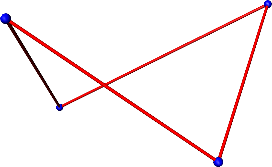
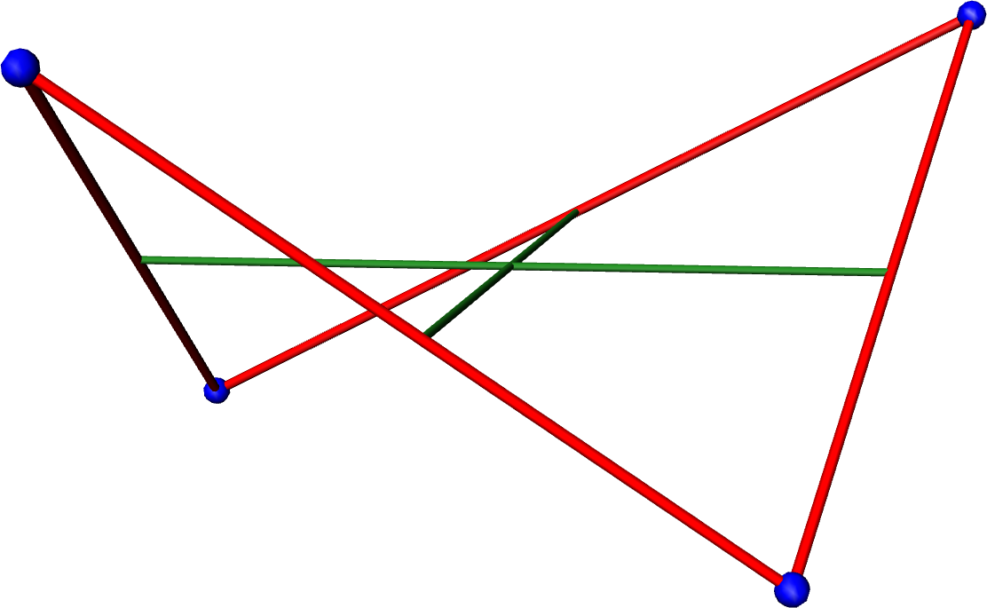
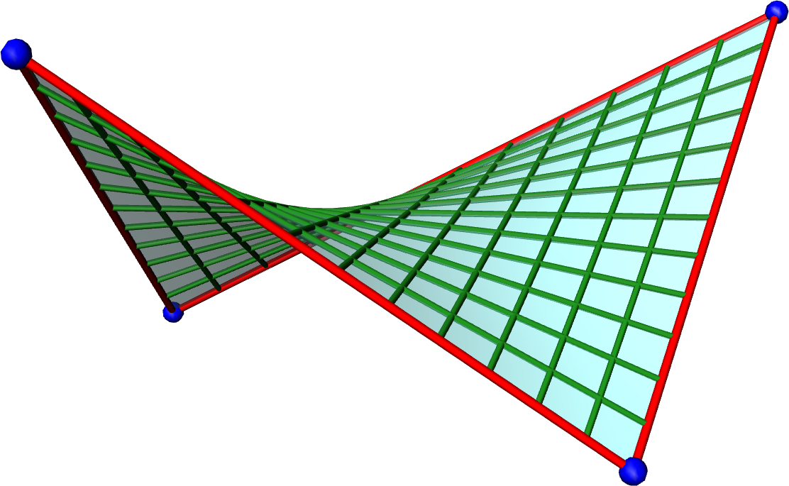
Figure 2. For a crisscrossed quadrilateral, there exists a unique doubly ruled quadric that contains the two crossing lines and the four edges of the supporting quadrilateral.

Going beyond the discretization of individual surfaces, another issue is the discretization of the class of transformations that is associated with classical A-surfaces. In general, the class of associated transformations and related permutability theorems are an essential aspect of specific “integrable” surface parametrizations, that is, surface parametrizations which admit underlying integrable structure [RS02]. In the case of A-nets, the associated transformations are called Weingarten transformations [Eis60, RS02]. Two continuous surfaces parametrized along asymptotic lines over the same domain are said to be Weingarten transforms of each other if the line connecting corresponding points is the intersection of the tangent planes to the two surfaces at these points. This relation carries over naturally to the setting of discrete A-nets in the following way (see, e.g., [Dol01, DNS01, Nie02]). For a discrete A-surface $f$ and a vertex $x$ of $f$, the plane containing the vertex star of $x$ is conveniently understood as the tangent plane to $f$ at $x$. Now let $\tilde{f}$ be another discrete A-surface with the same combinatorics as $f$. The A-surfaces $f$ and $\tilde{f}$ are said to form a discrete Weingarten pair if the line connecting corresponding vertices $x$ and $\tilde{x}$ is the intersection of the corresponding discrete tangent planes. Equivalently, this relation may be described as follows. Connecting corresponding vertices of $f$ and $\tilde{f}$, one obtains a 3-dimensional quadrilateral net $F$ that is composed of the two 2-dimensional layers $f$ and $\tilde{f}$. The surfaces $f$ and $\tilde{f}$ form a discrete Weingarten pair if and only if the net $F$ has planar vertex stars, which means that $F$ is a 3-dimensional A-net itself. This illustrates a well established discretization principle within discrete differential geometry, i.e., on the discrete level, surfaces and their transformations should be described by the same geometric or algebraic conditions. This approach reflects a deep and unifying understanding of the classical relations between parametrized surfaces and their transformations in the context of discrete integrability (see, e.g., [BS08]). It is worth mentioning that, analogous to the classical theory, two A-nets are discrete Weingarten transforms of each other if and only if their discrete Lelieuvre normals are related by a discrete Moutard transformation (see, e.g., [Dol01, DNS01, Nie02]).

The aim of the present article is to develop, in the context of hyperbolic nets, a canonical analogue of the classical and modern theories of Weingarten transformations for smooth and discrete A-surfaces respectively. Since hyperbolic nets possess the key features of both smooth and discrete A-surfaces, it is natural to demand that the same be true for their transformations. Thus, we here propose that two hyperbolic nets form a Weingarten pair if the supporting A-surfaces form a discrete Weingarten pair and, additionally, the hyperboloid patches associated with corresponding quadrilaterals are related by a classical Weingarten transformation. It turns out that this definition is indeed admissible but that the proof of this assertion is significantly more involved than the proof of the existence of both classical and discrete Weingarten transformations. Accordingly, we here confine ourselves to the investigation of single applications of Weingarten transformations and address the permutability properties (Bianchi diagram) of Weingarten transformations of hyperbolic nets and related aspects in a separate publication.

Structure and results of the present paper.

We begin in Section 2 with an overview of the aspects of the theory of discrete A-surfaces and their transformations which are relevant for our purposes. Subsequently, in Section 3, the description of hyperbolic nets recorded in [HVR13] is briefly reviewed and reformulated in terms of crisscrossed quadrilaterals. Particular attention is given to a scalar function $\rho$ defined at the vertices of a supporting A-net that describes crosses adapted to quadrilaterals of the support structure. In the case that the crosses encapsulate a hyperbolic net, the relation between this function $\rho$ and algebraic invariants composed of the discrete Moutard coefficients of the A-net is revealed. In Section 4, we develop the concept of Weingarten transformations of hyperbolic nets which constitute a subclass of more general Bäcklund transformations, the anlogues of which do not exist in the classical and discrete cases. We show how these may be characterized both geometrically in terms of crosses and algebraically in terms of the function $\rho$. It turns out that in the case of the generic Bäcklund transformation, the latter key function is governed by a non-autonomous version of the master discrete BKP (Miwa) equation of integrable systems theory [Miw82]. Moreover, it is demonstrated that, in the particular case of a Weingarten pair, $\rho$ may be identified with a potential for a particular choice of Moutard coefficients of a Lelieuvre representation associated with the underlying 2-layer 3D A-net. Accordingly, the above-mentioned BKP-type equation reduces to the standard discrete BKP equation which, in turn, gives rise to a novel geometric interpretation of Miwa’s fundamental equation.

It is important to note that a discrete A-surface may be extended to a hyperbolic net if and only if a certain condition on the twist of quadrilateral strips is satisfied. However, any A-surface with $\mathbb{Z}^{2}$ combinatorics is extendable in an analogous sense if the elementary quadrilaterals are equipped with whole hyperboloids rather than hyperboloid patches. Such nets, which still obey the tangency condition along edges, are termed pre-hyperbolic nets. Accordingly, our general approach is to introduce first Bäcklund and Weingarten transformations for pre-hyperbolic nets and then derive the theory for hyperbolic nets by taking into account the additional constraint on the quadrilateral strips. Here, the global existence of Weingarten pairs is proven by converting this constraint into a condition on the aforementioned algebraic invariants.

2. Discrete A-nets

In the following, we introduce the notion of discrete A-nets [Sau37, BS08] and summarize different aspects of the related theory that are important for our purpose. We start with the 2-dimensional case, i.e., discrete A-surfaces, and then move on to the higher-dimensional case, which is conveniently understood as the (integrable) theory of discrete A-surfaces and their associated transformations. This approach provides us with a structure which will be used as a guide when developing the analogous theory of hyperbolic nets and their transformations.

Notation.

For a discrete map defined on $\mathbb{Z}^{m}$, it is convenient to represent shifts in lattice directions by lower indices. Accordingly, for $z=(z_{1},\dots,z_{m})\in\mathbb{Z}^{m}$ and a map $\varphi$ on $\mathbb{Z}^{m}$, we write

$$\varphi_{1}(z):=\varphi(z_{1}+1,z_{2},\dots,z_{m}),\quad\varphi_{11}(z):=\varphi(z_{1}+2,z_{2},\dots,z_{m}),$$

$$\varphi_{2}(z):=\varphi(z_{1},z_{2}+1,z_{3},\dots,z_{m}),\quad\text{etc.}$$

Usually, we omit the argument for discrete maps and write

$$\varphi=\varphi(z),\quad\varphi_{1}=\varphi_{1}(z)\quad\text{etc.}$$

For $k\in\left\{1,\dots,m\right\}$ denote by $\mathcal{S}^{i_{1}\dots i_{k}}$ the $k$-dimensional subspace of $\mathbb{Z}^{m}$ that is spanned by directions $i_{1},\dots,i_{k}$,

$$\mathcal{S}^{i_{1}\dots i_{k}}=\operatorname{span}_{\mathbb{Z}}(e_{i_{1}},\dots,e_{i_{k}}),$$

where $e_{i}$ is the $i$-th unit vector in $\mathbb{Z}^{m}$. Finally, for $x_{1},\dots,x_{n}\in\mathbb{R}^{m}$ we denote by

$$\operatorname{inc}[x_{1},\dots,x_{n}]=\left\{\sum_{i=1}^{n}\alpha_{i}x_{i}\mid\sum_{i=1}^{n}\alpha_{i}=1\right\}$$

the affine subspace spanned by $x_{1},\dots,x_{n}$.

2.1. Discrete A-surfaces.

Definition 1 (Discrete A-surface).

A map $x:\mathbb{Z}^{2}\to\mathbb{R}^{3}$ is a called a 2-dimensional discrete A-net or discrete A-surface if for each $z\in\mathbb{Z}^{2}$ the point $x(z)$ is coplanar with all its neighbours. The points $x(\mathbb{Z}^{2})$ are synonymously called lattice points or vertices of $x$. The line segments connecting adjacent lattice points $x(z)$ and $x(\tilde{z})$ are called edges of $x$. A vertex together with all its neighbours is called a vertex star and we call a plane supporting a vertex star a vertex plane.

Remark 2.

In order to describe an A-surface $x$ with more general combinatorics than $\mathbb{Z}^{2}$, one uses quad-graphs, i.e., strongly regular cell decompositions of topological surfaces with all 2-cells being quadrilaterals, as domain for $x$.

Genericity assumption.

We assume that the A-nets are generic, i.e., elementary quadrilaterals are skew and each vertex star defines a unique vertex plane.

Lelieuvre representation of A-surfaces.

Let $m$ be any normal field to the vertex planes of a discrete A-surface $x:\mathbb{Z}^{2}\to\mathbb{R}^{3}$. Planarity of vertex stars implies that the edges of $x$ can be described as

(1) $$x_{i}-x=\alpha^{i}\ m_{i}\times m,\quad i=1,2.$$

The compatibility condition of (1) implies that

$$\alpha^{1}\alpha^{1}_{2}=\alpha^{2}\alpha^{2}_{1},$$

which guarantees the existence of a potential $\xi$ such that

$$\alpha^{i}=\xi_{i}\xi.$$

Introducing $n=\xi m$, the description (1) of edges simplifies to

(2) $$x_{i}-x=n_{i}\times n,\quad i=1,2.$$

The map $n:\mathbb{Z}^{2}\to\mathbb{R}^{3}$ is called a discrete Lelieuvre normal field and (2) are called discrete Lelieuvre formulae. The corresponding simplified compatibiliy condition is the discrete Moutard-type equation

(3) $$n_{12}-n=a^{12}(n_{2}-n_{1}),$$

with scalars $a^{12}$ that are called (discrete) Moutard coefficients (see, e.g., [NS97, BS99a, Dol01, DNS01, Nie02]).

Lelieuvre normals are unique up to black-white rescaling. This means that given a Lelieuvre representation $n$ of an A-net $x:\mathbb{Z}^{2}\to\mathbb{R}^{3}$, one can colour the vertices of $\mathbb{Z}^{2}$ black and white such that adjacent vertices are of different colour and for arbitrary $\alpha\neq 0$ define

(4) $$\tilde{n}=\begin{cases}\alpha n&\text{on black vertices},\\ \frac{1}{\alpha}n&\text{on white vertices}.\end{cases}$$

Then $\tilde{n}$ is another Lelieuvre representation of the same A-net $x$. Solutions of the Moutard equation (3) are in one-to-one correspondence with discrete A-nets modulo global translation of $x$ and black-white rescaling of $n$.

In a fixed Lelieuvre representation $n$, there are four related Moutard coefficients associated with each elementary quadrilateral. They correspond to different equivalent reformulations of (3). We identify those coefficients with combinatorial pictures as shown in Fig. 3.

Figure 3. Identification of Moutard coefficients with combinatorial pictures. The long oriented diagonal represents the vector which is written as a scalar multiple of the short oriented diagonal. Changing the orientation of one vector corresponds to a sign change of the Moutard coefficient, $a\to-a$. Interchanging the long and the short diagonal results in the reciprocal value, $a\to\frac{1}{a}$.

Invariants associated with pairs of edge-adjacent quadrilaterals of an A-net.

Changing the Lelieuvre representation of an A-net, i.e., performing a black-white rescaling (4) of a given Lelieuvre normal field $n$, changes the Moutard coefficients as indicated in Fig. 4. Note that the sign of the Moutard coefficient is preserved.

Figure 4. Rescaling of Moutard coefficients induced by a b/w-rescaling of Lelieuvre normals.

A Moutard coefficient becomes rescaled by $\alpha^{2}$ or $\frac{1}{\alpha^{2}}$, depending on the type (black-black or white-white) of the associated long diagonal. This yields algebraic invariants associated with edge-adjacent quadrilaterals of a discrete A-net as certain products of Moutard coefficients. One type of invariant that turns out to be crucial for our purpose is characterized by the following

Definition 3 (Parallel invariants).

Let $a$ and $\tilde{a}$ be Moutard coefficients associated with edge-adjacent quadrilaterals of an A-net. If, in the symbolic representation of Fig. 3, the coefficients $a$ and $\tilde{a}$ are related by a “parallel transport” then the algebraic invariant $a\tilde{a}$ of the A-net is called a parallel invariant (cf. Fig. 5).

Figure 5. Products $a\tilde{a}$ of Moutard coefficients that are related by a parallel transport are algebraic invariants associated with pairs of edge-adjacent quadrilaterals of an A-net.

Remark 4.

Moutard coefficients $a^{12}$ and $a^{12}_{i},i=1,2$ associated with edge-adjacent quadrilaterals of an A-surface $x:\mathbb{Z}^{2}\to\mathbb{R}^{3}$ yield parallel invariants $a^{12}a^{12}_{i}$.

Cauchy problem for A-surfaces.

The Lelieuvre representation provides a very convenient description of Cauchy problems for A-surfaces. Admissible Cauchy data for an A-surface $x:\mathbb{Z}^{2}\to\mathbb{R}^{3}$ are, for example,

(5) $$n(\mathcal{S}^{i}),\ i=1,2;\quad a^{12}(\mathbb{Z}^{2});\quad x_{0}.$$

Thus, Moutard coefficients $a^{12}$ may be prescribed for the whole surface. This allows to determine the entire Lelieuvre normal field from initial values of $n$ along the coordinate axes $\mathcal{S}^{1}$ and $\mathcal{S}^{2}$, using (3). Due to (2), the A-surface $x$ is then determined up to translation so that only one vertex $x_{0}$ of $x$ is needed to complete the Cauchy data.

Continuum limit.

According to the classical theory, a surface $x:\mathbb{R}^{2}\to\mathbb{R}^{3}$ parametrized along asymptotic lines can be described by its Lelieuvre normal $n:\mathbb{R}^{2}\to\mathbb{R}^{3}$ as stated by the Lelieuvre formulae

(6) $$\partial_{1}x=\partial_{1}n\times n,\quad\partial_{2}x=n\times\partial_{2}n.$$

In the continuous case, the Lelieuvre normal is unique up to sign and does not allow a rescaling as in the discrete case. The compatibility condition of (6) is the classical Moutard equation

(7) $$\partial_{1}\partial_{2}n=q^{12}n.$$

To obtain (6),(7) as a continuum limit of (2),(3), one first has to change the orientation of the discrete Lelieuvre normals according to, for example, $n\to(-1)^{z_{2}}n.$ This converts (2) and (3) into

(8) $$x_{1}-x=n_{1}\times n,\quad x_{2}-x=n\times n_{2},\quad n_{12}+n=a^{12}(n_{2}+n_{1}),$$

which leads to (6) and (7) by expressing equations (8) in terms of difference quotients and then taking the limit. Indeed, it is easily verified that without suitable flipping of Lelieuvre normals, the system (2) does not possess a simultaneous continuum limit.

2.2. Higher-dimensional A-nets

There are two philosophically different approaches to introducing higher-dimensional A-nets. The first approach generalizes the incidence geometric structure, i.e., it generalizes the idea of planar vertex stars to an $m$-dimensional lattice with $m\geq 3$. The second approach emphasizes the relation between A-surfaces and their transformations. Starting with the notion of 2-dimensional discrete A-surfaces, one imposes planarity of vertex stars only on 2-dimensional layers of an $m$-dimensional lattice. A multidimensional A-net is then understood as a family of A-surfaces which are interrelated according to the same geometric property that characterizes the surfaces themselves.

However, it is not difficult to see that the seemingly weaker condition of planar vertex stars in every 2-dimensional layer is equivalent to planarity of the whole vertex stars. Indeed, it is noted that, for a generic net, three consecutive points along a discrete coordinate line are not collinear. Therefore, three such vertices already span the vertex plane at the middle vertex for all 2-dimensional sublattices that contain this coordinate line. Applying this argument repeatedly, one finds that, at a fixed vertex, all vertex planes associated with different 2-dimensional coordinate planes through that vertex coincide.

It is easy to verify that for a higher-dimensional lattice with all 2-cells being quadrilaterals, planarity of vertex stars implies that the whole lattice is contained in the 3-dimensional space that is spanned by the vertices of one arbitrary elementary quadrilateral. Therefore, it is no restriction do define A-nets of arbitrary dimension as maps $x:\mathbb{Z}^{m}\to\mathbb{R}^{3}$ with planar vertex stars. Verifying the existence of 2-dimensional A-nets is straight forward since it is not difficult to perform an iterative geometric construction of A-surfaces which contains sufficiently many degrees of freedom at each step. But, in the higher-dimensional case, it is not obvious that the condition of planar vertex stars can be imposed consistently even on a 3D lattice. Already for a single hexahedron of a 3D lattice one obtains a closure condition. While it is clear that one can choose 7 points associated with 7 vertices of a 3D cube such that all 7 vertex stars are planar, the 7 points determine 4 planes that have to intersect in a single point, i.e., the missing eighth vertex. The existence of this unique intersection point is guaranteed by

Theorem 5 (Cox’ theorem).

Let $P_{1},P_{2},P_{3},P_{4}$ be four planes in $\mathbb{R}\textup{P}^{3}$ which intersect in a point $x$. Let $x_{ij}\in P_{i}\cap P_{j},i\neq j$, be six points on the lines of intersection of these planes and define four new planes $P_{ijk}=\operatorname{inc}[x_{ij},x_{jk},x_{ik}]$. Then, the four planes $P_{123},P_{124},P_{134},P_{234}$ intersect in one point $x_{1234}$ (cf. Fig. 6).

For a proof of Theorem 5, see, e.g., [BS08].

Figure 6. A Cox configuration of points $x$ and planes $P$ that are associated with vertices of a 4D cube. An edge connecting a point and a plane represents incidence. There are four planes passing through each point and each plane contains four points. There are four ways of interpreting a 4D Cox configuration as an elementary hexahedron of an A-net, each corresponding to the contraction of all edges of one coordinate direction.

According to the previous considerations, we say that A-nets are governed by a 3D system in the following sense: feasible data at seven vertices of an elementary hexahedron determine the data at the remaining vertex uniquely, where “feasible data” refers to lattice points that satisfy the condition of planar vertex stars. As a consequence, feasible initial data along three intersecting coordinate planes of $\mathbb{Z}^{3}$ determine the net on the whole of $\mathbb{Z}^{3}$.

Moreover, the 3D system governing discrete A-nets is multidimensionally consistent, i.e., it can be imposed consistently on higher-dimensional lattices $\mathbb{Z}^{m}$. The most elementary building block for this is a 4D cube as in Fig. 7, right. Prescribing feasible initial data at the 11 vertices $z,z_{1},\dots,z_{34}$ yields, in a first step, the data at the four vertices $z_{123},z_{124},z_{134},z_{234}$. Subsequently, there exist four different ways of determining the data at $z_{1234}$ as this vertex is the intersection of four different 3D cubes. The fact that the potentially different data at $z_{1234}$ coincide for arbitrary feasible initial data is called 4D consistency of the 3D system. In general, ($m+1$)D consistency of an $m$D system implies consistency in arbitrary dimension. Multidimensional consistency is understood as discrete integrability and we say that the 3D system governing A-nets is discrete integrable (see [BS08] and references therein).

Figure 7. Left: The data of a discrete A-net at seven vertices $z,z_{1},\dots,z_{23}$ of a 3D cube determine the data at the eighth vertex $z_{123}$. Right: The 3D system describing A-nets can be imposed consistently on a 4D cube.

Algebraic description of higher-dimensional A-nets.

As in the 2-dimensional case, discrete A-nets $x:\mathbb{Z}^{m}\to\mathbb{R}^{3}$ can be described by their Lelieuvre normals $n:\mathbb{Z}^{m}\to\mathbb{R}^{3}$,

(9) $$x_{i}-x=n_{i}\times n,\quad i=1,\dots,m.$$

In the multidimensional case, Lelieuvre normals satisfy a system of discrete Moutard equations [NS97]

(10) $$n_{ij}-n=a^{ij}(n_{j}-n_{i}),\quad i\neq j,$$

with skew-symmetric Moutard coefficients $a^{ji}=-a^{ij}$. The Moutard coefficients are not independent but, since A-nets are described by a 3D system, satisfy the following relation (compatibility condition) on each elementary hexahedron of $\mathbb{Z}^{m}$

(11) $$a^{ij}_{k}=-\frac{a^{ij}}{a^{ij}a^{jk}+a^{jk}a^{ki}+a^{ki}a^{ij}},\quad i\neq j\neq k\neq i.$$

The coefficients $a^{ij}$ are understood as fields on elementary quadrilaterals of $(i,j)$-coordinate planes, where a lower index $k$ represents a shift of the variable $a^{ij}$ in the $k$-th coordinate direction. The multidimensional consistency of A-nets can be stated on an algebraic level as the multidimensional consistency of equation (11).

The Moutard coefficients of a multidimensional A-net can be parametrized by a function $\tau$ at vertices. More precisely, choosing an ordering for each pair of distinct lattice directions, for example lexicographic ordering $i<j$, selects one type of Moutard coefficients for each coordinate plane. Then, there exists a (non-unique) function $\tau:\mathbb{Z}^{m}\to\mathbb{R}$ such that the selected Moutard coefficients can be written as

(12) $$a^{ij}=\frac{\tau_{i}\tau_{j}}{\tau\tau_{ij}}.$$

It is a necessary and sufficient condition for the existence of a potential $\tau$ that satisfies (12) that for each 3D cube the ratios of Moutard coefficients associated with opposite faces coincide. This is the case, since (11) implies that

(13) $$\frac{a^{ij}}{a^{ij}_{k}}=\frac{a^{jk}}{a^{jk}_{i}}=\frac{a^{ki}}{a^{ki}_{j}}=-(a^{ij}a^{jk}+a^{jk}a^{ki}+a^{ki}a^{ij}).$$

Indeed, if we regard (12) as a definition of $\tau_{ij}$, it is not difficult to see that the associated compatibility conditions

$$(\tau_{ij})_{k}=(\tau_{ik})_{j}=(\tau_{jk})_{i}$$

are satisfied modulo $a^{ij}/a^{ij}_{k}=a^{jk}/a^{jk}_{i}=a^{ki}/a^{ki}_{j}$.

The system (11) for Moutard coefficients on a 3-dimensional sublattice is equivalent to a discrete BKP (Miwa) equation [Miw82] for $\tau$ on that sublattice. In the lexicographic case, i.e., Moutard coefficients parametrized according to (12) with $1\leq i<j\leq m$, system (11) reduces to the Miwa equation in the form

(14) $$\tau\tau_{ijk}-\tau_{i}\tau_{jk}+\tau_{j}\tau_{ik}-\tau_{k}\tau_{ij}=0,\quad i<j<k.$$

Different sets of Moutard coefficients parametrized by $\tau$ may yield different relative signs in (14), and, in general, one obtains different signs for different 3-dimensional sublattices. Having observed this, it is worth mentioning that equation (14) is a multidimensionally consistent equation, i.e., it can be imposed simultaneously on each 3-dimensional sublattice of a lattice $\mathbb{Z}^{m}$ of arbitrary dimension.

Cauchy problem for multidimensional A-nets.

Using (11) as evolution equation for Moutard coefficients, it is clear how to extend Cauchy data (5) for A-surfaces to Cauchy data for multidimensional A-nets $x:\mathbb{Z}^{m}\to\mathbb{R}^{3}$. One obtains, for example,

(15) $$n(\mathcal{S}^{i}),\ i=1,\dots,m;\quad a^{ij}(\mathcal{S}^{ij}),\ 1\leq i<j\leq m;\quad x_{0}.$$

Continuum limit.

For an A-net $x:\mathbb{Z}^{m}\to\mathbb{R}^{3},m\geq 3$, it is only possible to take the continuum limit in at most two coordinate directions. Recalling the 2-dimensional case, for fixed $i,j$, it is necessary to flip Lelieuvre normals such that, e.g.,

$$x_{i}-x=n_{i}\times n,\quad x_{j}-x=n\times n_{j}$$

in order to obtain a continuum limit in the $(i,j)$-coordinate planes. To this end, start with a discrete Lelieuvre normal $n$ satisfying (9) and perform a flip of every second Lelieuvre normal in direction $j$,

$$n\to(-1)^{z_{j}}n.$$

In the continuum limit of $i$ and $j$ directions, one obtains classical A-surfaces as $(i,j)$-coordinate planes of the resulting semi-discrete $m$-dimensional A-net. However, it is not possible to perform another continuum limit in a direction $k\neq i,j$ since, either in the $(i,k)$-planes or in the $(j,k)$-planes, the limit does not exist. In fact, there do not exist higher-dimensional continuous A-nets beyond A-surfaces.

2.3. Weingarten transformations of discrete A-surfaces

An essential aspect of privileged surface parametrizations such as conjugate, curvature, or asymptotic line parametrizations is the corresponding class of transformations. The transformations associated with a specific class of parametrization preserve that type of parametrization. In the context of surfaces parametrized along asymptotic lines, the corresponding transformations are called Weingarten transformations [Eis60, RS02]. Two continuous A-surfaces are said to be Weingarten transforms of each other if the line connecting corresponding points is the intersection of the tangent planes to the two surfaces at these points. A literal discretization of classical Weingarten transformations (see, e.g., [Dol01, DNS01, Nie02]) yields

Definition 6 (Weingarten transformation of discrete A-surfaces / Weingarten property).

Two discrete A-surfaces $f,\tilde{f}:\mathbb{Z}^{2}\to\mathbb{R}^{3}$ are related by a Weingarten transformation if for every $z\in\mathbb{Z}^{2}$ the line $\operatorname{inc}[f(z),\tilde{f}(z)]$ is the intersection of the vertex planes of $f$ and $\tilde{f}$ at the points $f(z)$ and $\tilde{f}(z)$, respectively. The net $\tilde{f}$ is called a Weingarten transform of the net $f$ (and vice versa) and $f,\tilde{f}$ are said to form a Weingarten pair. We say that the Weingarten property is satisfied at pairs $f(z),\tilde{f}(z)$ of corresponding points.

It is a remarkable fact that many classes of special surface parametrizations and their associated transformations can be unified at the discrete level. This means that surfaces and their transformations become indistinguishable in the sense that they are described by the same geometric properties or, algebraically, by the same equations. Definition 6 clearly illustrates this unification: Discrete A-surfaces $f,\tilde{f}:\mathbb{Z}^{2}\to\mathbb{R}^{3}$ form a Weingarten pair if and only if $F:\mathbb{Z}^{2}\times\left\{0,1\right\}$ composed of the layers $F(\cdot,0)=f$ and $F(\cdot,1)=\tilde{f}$ constitutes a 3-dimensional A-net.

3. Hyperbolic nets in terms of crisscrossed quadrilaterals

We begin with the introduction of hyperboloids and hyperboloid patches before explaining the notion of hyperbolic nets and recapitulating previous results. Subsequently, we give an elementary geometric description of those results, which will be the starting point for our discussion of transformations of hyperbolic nets.

3.1. Hyperboloids and hyperboloid patches

A hyperboloid in our sense is a doubly ruled quadric in $\mathbb{R}^{3}$, i.e., a hyperboloid of one sheet or a hyperbolic paraboloid. This terminology is justified by projective geometry since, in $\mathbb{R}\textup{P}^{3}$, there exists only one type of doubly ruled quadric. Referring to an affine chart which embeds $\mathbb{R}^{3}\subset\mathbb{R}\textup{P}^{3}$, one may say that a doubly ruled quadric in $\mathbb{R}\textup{P}^{3}$ appears as a hyperbolic paraboloid in the affine part $\mathbb{R}^{3}$ if it is tangent to the ideal plane at infinity, otherwise it appears as a hyperboloid of one sheet. In general, if a surface contains a straight line, obviously this line is an asymptotic line, following a constant direction of vanishing normal curvature. Moreover, it is an essential fact of elementary projective geometry that any three mutually skew lines determine a unique hyperboloid.

Definition 7 (Hyperboloid patch / ruling / regulus).

A hyperboloid patch is a (parametrized) surface patch obtained by restricting an asymptotic line parametrization $f:D\to\mathbb{R}^{3}$ of a hyperboloid to a closed rectangle. We call an asymptotic line of a hyperboloid also a ruling. Each of the two families of rulings that cover a hyperboloid is called a regulus.

Geometrically, a hyperboloid patch is a piece of a hyperboloid cut out along four asymptotic lines (cf. Fig. 8, left). Note that not any four asymptotic lines of a hyperboloid bound a finite hyperboloid patch. More precisely, four asymptotic lines, two from each regulus, divide each other into several line segments, four of them being finite. There exists a patch that is bounded by those finite segments if and only if a ruling of the hyperboloid that intersects one finite segment also intersects the opposite finite segment (see Fig. 8).

Figure 8. Left: A finite hyperboloid patch. Right: A finite skew quadrilateral on a hyperboloid that does not bound a hyperboloid patch.

Definition 8 (Adapted hyperboloids / Tangency or $C^{1}$-condition).

We call a hyperboloid (patch) adapted to a skew quadrilateral if the edges of the quadrilateral are asymptotic lines of the hyperboloid (patch). Moreover, we say that two hyperboloids (hyperboloid patches) adapted to edge adjacent skew quadrilaterals satisfy the tangency condition, or $C^{1}$-condition for short, if the tangent planes of the two surfaces coincide along the common asymptotic line.

3.2. Previous results

In the following, we give a brief overview of the work [HVR13], which introduced hyperbolic nets as a novel discretization of smooth A-surfaces.

Definition 9 (Hyperbolic and pre-hyperbolic nets).

Hyperbolic nets are piecewise smooth surfaces which are composed of hyperboloid surface patches that are adapted to the skew quadrilaterals of a supporting A-net and satisfy the $C^{1}$-condition. A pre-hyperbolic net, in turn, consists of complete adapted hyperboloids that satisfy the $C^{1}$-condition.

Remark 10.

Hyperbolic nets may be regarded as “$C^{1}$-versions” of smooth A-surfaces, whereby, for convenience, we do not exclude the occurrence of two adjacent hyperboloid patches forming a cusp. Indeed, cusps are common singularities of pseudospherical surfaces which form an important class of A-surfaces in the sense that these are naturally parametrized in terms of asymptotic coordinates. Furthermore, as seen in Fig 9, the discrete A-surface which becomes extended to a (pre-)hyperbolic net may be of more general quad-graph combinatorics than $\mathbb{Z}^{2}$.

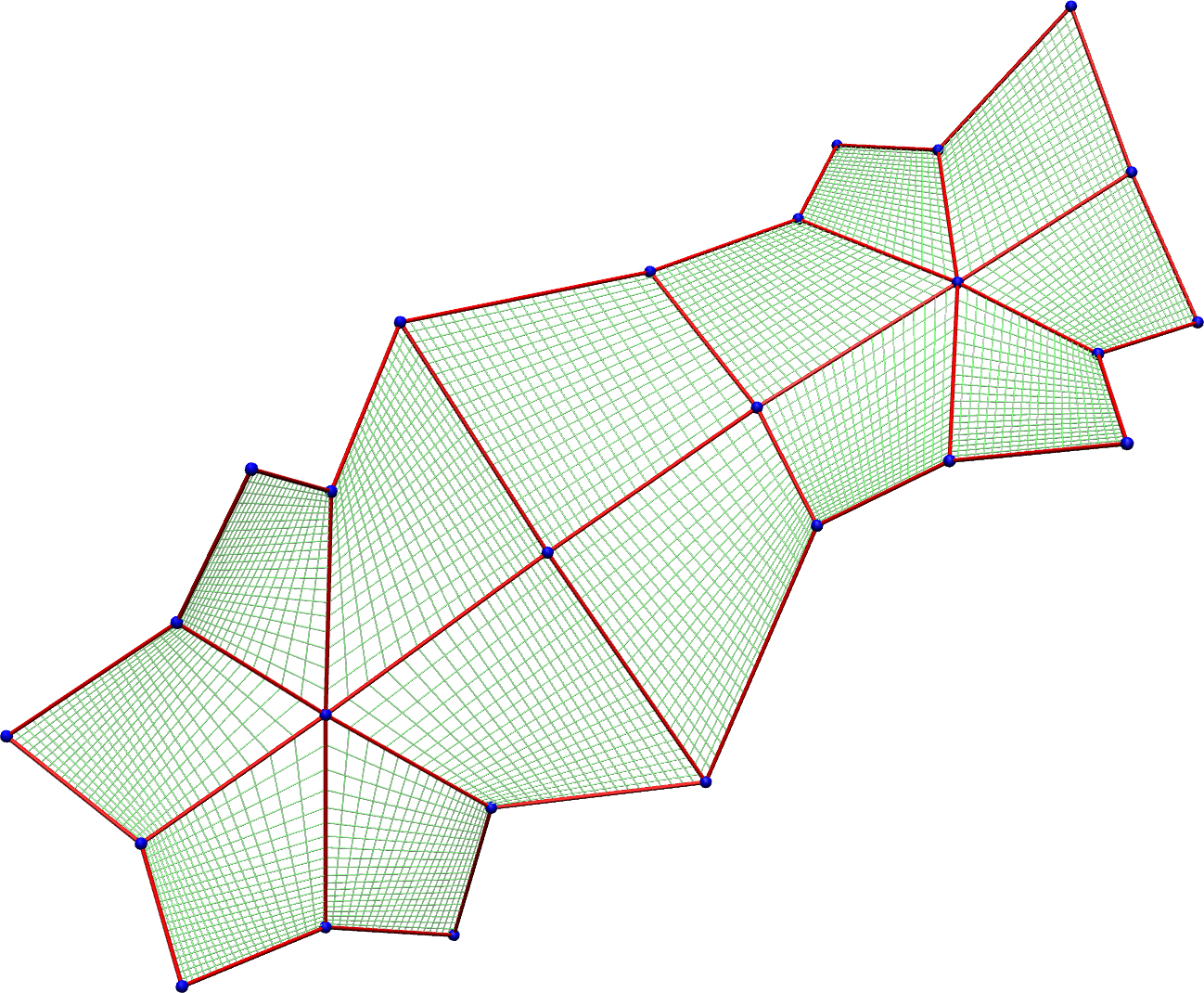
Figure 9. Two perspectives of a hyperbolic net with two vertices of degree six.

Given two edge adjacent skew quadrilaterals and a hyperboloid adapted to one of them, the $C^{1}$-condition determines a unique hyperboloid adapted to the other quadrilateral. Accordingly, for a given A-net one may choose one inital adapted hyperboloid and then propagate this hyperboloid to all other quadrilaterals of the net by imposing the $C^{1}$-condition on adjacent hyperboloids. The question is whether this propagation is globally consistent, i.e., path-independent, so that a supporting A-surface can be extended to a well-defined pre-hyperbolic net. It turns out that a simply connected discrete A-surface is extendable to a pre-hyperbolic net if and only if all interior vertices are of even degree. If we regard “consecutive” edges of a discrete A-surface as discrete asymptotic lines then this is consistent with the classical theory since asymptotic lines on continuous A-surfaces do not terminate.

Now, if we proceed from pre-hyperbolic nets to hyperbolic nets then the essential difference is the following. In the context of pre-hyperbolic nets, the propagation of adapted hyperboloids according to the $C^{1}$-condition is always possible locally, while for hyperboloid patches this is not true. More precisely, given two edge-adjacent skew quadrilaterals $Q,\tilde{Q}$ and a hyperboloid $\mathcal{H}$ adapted to $Q$, the $C^{1}$-condition yields a unique hyperboloid $\tilde{\mathcal{H}}$ adapted to $\tilde{Q}$. But, as explained in Section 3.1, not every hyperboloid adapted to a skew quadrilateral can be restricted to a patch that is bounded by the quadrilateral. It may happen that $\mathcal{H}$ can be restricted to a patch bounded by $Q$, but that the quadrilateral $\tilde{Q}$ does not bound a patch on $\tilde{\mathcal{H}}$. In [HVR13] it was shown that, assuming that $Q$ bounds a patch on $\mathcal{H}$, the hyperboloid $\tilde{\mathcal{H}}$ can be restricted to a patch bounded by $\tilde{Q}$ if and only if the quadrilaterals $Q$ and $\tilde{Q}$ are equi-twisted. Roughly speaking, the twist of a pair of opposite edges of a skew quadrilateral indicates in which direction an edge turns if it is transported into the opposite edge along the two remaining edges. (The twists of the two pairs of edges are always complementary.) Two edge-adjacent quadrilaterals are then called equi-twisted if the twist of corresponding pairs of edges coincides. Accordingly, the notion of equi-twist gives rise to equi-twisted quadrilateral strips (cf. Fig. 10).

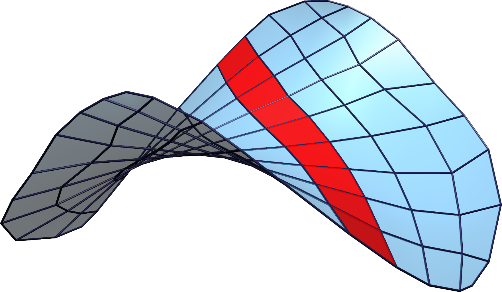
Figure 10. An equi-twisted quadrilateral strip of an A-net.

A discrete A-surface for which all quadrilateral strips are equi-twisted is called equi-twisted for brevity. It is not difficult to see that, for an equi-twisted A-surface, all interior vertices are of even degree. It follows that a simply connected discrete A-surface can be extended to a hyperbolic net if and only if it is equi-twisted. Moreover, for any skew quadrilateral there exists a 1-parameter family of adapted hyperboloid patches. Since the $C^{1}$-propagation is unique modulo the initial patch, one obtains a 1-parameter family of adapted hyperbolic nets for an equi-twisted A-surface.

In [HVR13], A-nets, hyperboloids and the extension of A-nets to (pre-)hyperbolic nets are all described within the projective model of Plücker line geometry. In that model, lines in $\mathbb{R}\textup{P}^{3}$ are represented by points on the Plücker quadric, which is a 4-dimensional quadric embedded in a 5-dimensional projective space. The key feature of the model is that two lines in $\mathbb{R}\textup{P}^{3}$ intersect if and only if their representatives in the Plücker quadric are polar with respect to the quadric. In the Plücker setting, A-nets are discrete line congruences in the Plücker quadric and the reguli of hyperboloids appear as non-degenerate conic sections of the Plücker quadric with 2-planes. For the purpose of this paper, it is now appropriate to re-establish the theory of hyperbolic nets in affine $\mathbb{R}^{3}$ on a purely elementary geometric level.

3.3. Hyperboloids and hyperboloid patches as skew quadrilaterals equipped with crisscrossing lines.

A skew quadrilateral in $\mathbb{R}^{3}$ consists of four points in general position that are connected by finite edges. A crisscrossed quadrilateral is a skew quadrilateral $Q$ that is equipped with a pair of intersecting lines as shown in Fig. 11. A pair of such lines, which we call a cross, is determined by the corresponding quadruple of coplanar intersection points with the extended edges of $Q$. We refer to those intersection points as cross vertices and call the intersection point of the two lines the centre of the cross. If a cross vertex is not only contained in an extended edge but in the edge itself, we call it an internal cross vertex. If all four vertices of a cross are internal, we say that $Q$ is equipped with an internal cross as in the example of Fig. 11. It is noted that coplanarity of the cross vertices implies that the number of internal cross vertices is always even.

Figure 11. A skew quadrilateral that is equipped with an internal cross.

For any given skew quadrilateral $Q$, there exists a 1-parameter family of adapted hyperboloids (cf. Definition 8). Since a hyperboloid is determined by three skew lines, extending $Q$ to a crisscrossed quadrilateral determines a unique adapted hyperboloid, where a 2-parameter family of crosses belongs to the same adapted hyperboloid. Not every hyperboloid adapted to $Q$ can be restricted to a patch bounded by $Q$, as indicated in Fig. 8, right. The restriction is possible if and only if there exists an internal cross that encodes the adapted hyperboloid. Therefore, hyperboloid patches adapted to $Q$ can be conveniently described by internal crosses.

The extension of a skew quadrilateral $Q=(x_{1},x_{2},x_{3},x_{4})$ to a crisscrossed quadrilateral is determined by the choice of three cross vertices on three extended edges, say $p_{12},p_{23},p_{34}$ in the notation of Fig. 11. The fourth vertex $p_{41}$ is then obtained as the intersection of the plane $\operatorname{inc}[p_{12},p_{23},p_{34}]$ with the fourth extended edge. The three vertices $p_{12},p_{23},p_{34}$ can be described as affine combinations of the points $x_{1},x_{2},x_{3},x_{4}$. For this purpose, introduce scalars $\rho_{1},\rho_{2},\rho_{3},\rho_{4}$ at vertices such that

(16) $$p_{12}=\frac{\rho_{1}x_{1}+\rho_{2}x_{2}}{\rho_{1}+\rho_{2}},\quad p_{23}=\frac{\rho_{2}x_{2}+\rho_{3}x_{3}}{\rho_{2}+\rho_{3}},\quad p_{34}=\frac{\rho_{3}x_{3}+\rho_{4}x_{4}}{\rho_{3}+\rho_{4}}.$$

The $\rho_{i}$ are unique up to homogeneous scaling, $\rho_{i}\to\alpha\rho_{i},\ \alpha\neq 0$. Ratios of these scalars correspond to ratios of oriented lengths that involve adjacent vertices of $Q$ and the cross vertex on the corresponding extended edge. For example

$$p_{12}=x_{1}+\frac{\rho_{2}}{\rho_{1}+\rho_{2}}(x_{2}-x_{1})=x_{2}+\frac{\rho_{1}}{\rho_{1}+\rho_{2}}(x_{1}-x_{2})$$

$$\iff x_{2}=p_{12}+\frac{\rho_{1}}{\rho_{1}+\rho_{2}}(x_{2}-x_{1}).$$

Therefore,

$$l(x_{1},p_{12})=\frac{\rho_{2}}{\rho_{1}+\rho_{2}}l(x_{1},x_{2})\quad\text{and}\quad l(p_{12},x_{2})=\frac{\rho_{1}}{\rho_{1}+\rho_{2}}l(x_{1},x_{2}),$$

which yields

$$\frac{l(x_{1},p_{12})}{l(p_{12},x_{2})}=\frac{\rho_{2}}{\rho_{1}}.$$

In the same manner, one obtains

$$\frac{l(x_{2},p_{23})}{l(p_{23},x_{3})}=\frac{\rho_{3}}{\rho_{2}},\quad\frac{l(x_{3},p_{34})}{l(p_{34},x_{4})}=\frac{\rho_{4}}{\rho_{3}}.$$

The point $p_{41}$ lies in the plane spanned by $p_{12},p_{23}$, and $p_{34}$ if and only if it is related to $x_{1}$ and $x_{4}$ in an analogous manner, that is,

(17) $$\frac{l(x_{4},p_{41})}{l(p_{41},x_{1})}=\frac{\rho_{1}}{\rho_{4}}\quad\iff\quad p_{41}=\frac{\rho_{4}x_{4}+\rho_{1}x_{1}}{\rho_{4}+\rho_{1}}.$$

This assertion is a consequence of the following theorem for $n=4$.

Theorem 11 (Generalized Menelaus Theorem).

Let $x_{1},...,x_{n+1}$ be $n+1$ points in general position in $\mathbb{R}^{n}$, i.e., $\operatorname{inc}[x_{1},\dots,x_{n+1}]=\mathbb{R}^{n}$. Let $p_{i,i+1}$ be some points on the lines $\operatorname{inc}[x_{i},x_{i+1}]$ different from $x_{i},x_{i+1}$ (indices are taken modulo $n+1$). The $n+1$ points $p_{i,i+1}$ lie in an affine hyperplane if and only if the following relation for the quotients of directed lengths holds:

$$M(x_{1},p_{1,2},\dots,x_{n+1},p_{n+1,1}):=\prod_{i=1}^{n+1}\frac{l(x_{i},p_{i,i+1})}{l(p_{i,i+1},x_{i+1})}=(-1)^{n+1}.$$

For a proof of Theorem 11 see, e.g., [BS08].

On use of (16) and (17), it is easily verified that the centre $p$ of the cross is given by

$$p=\operatorname{inc}[p_{12},p_{34}]\cap\operatorname{inc}[p_{23},p_{41}]=\frac{\rho_{1}x_{1}+\rho_{2}x_{2}+\rho_{3}x_{3}+\rho_{4}x_{4}}{\rho_{1}+\rho_{2}+\rho_{3}+\rho_{4}}.$$

It is important to note that $\rho_{1},\rho_{2},\rho_{3},\rho_{4}$ describe an internal cross if and only if they have the same sign, which follows from the observation that a cross vertex is internal if and only if the two corresponding $\rho$s have the same sign. More general, an adapted hyperboloid can be restricted to a patch that is bounded by the supporting quadrilateral if for each pair of opposite cross vertices either both vertices are internal, or both vertices are external. If this holds for one pair, it automatically holds for the other pair as well. Therefore, the scalars $\rho_{1},\rho_{2},\rho_{3},\rho_{4}$ determine a restrictable hyperboloid if and only if $\rho_{1}\rho_{2}\rho_{3}\rho_{4}>0$.

Denote by

$$\operatorname{cr}(a,b,c,d)=\frac{l(a,b)}{l(b,c)}\frac{l(c,d)}{l(d,a)}$$

the cross-ratio of four collinear points and let $\tilde{p}_{ij}$ be four additional cross vertices that are determined by scalars $\tilde{\rho}_{i}$. It is a fact of elementary projective geometry that the lines $\operatorname{inc}[p_{12},p_{34}]$ and $\operatorname{inc}[\tilde{p}_{12},\tilde{p}_{34}]$ determine the same adapted hyperboloid if and only if the cross-ratios

$$\operatorname{cr}(x_{1},p_{12},x_{2},\tilde{p}_{12})=\frac{\rho_{2}}{\rho_{1}}\cdot\frac{\tilde{\rho}_{1}}{\tilde{\rho}_{2}}\quad\text{and}\quad\operatorname{cr}(x_{4},p_{34},x_{3},\tilde{p}_{34})=\frac{\rho_{3}}{\rho_{4}}\cdot\frac{\tilde{\rho}_{4}}{\tilde{\rho}_{3}}$$

coincide. Summing up the previous considerations, we have established

Lemma 12.

The extension of a skew quadrilateral $Q=(x_{1},x_{2},x_{3},x_{4})$ in $\mathbb{R}^{3}$ to a crisscrossed quadrilateral (cf. Fig. 11) corresponds to the choice of scalars $\rho_{1},\rho_{2},\rho_{3},\rho_{4}$ associated with the vertices of $Q$. The vertices of the cross are then parametrized by

$$p_{12}=\frac{\rho_{1}x_{1}+\rho_{2}x_{2}}{\rho_{1}+\rho_{2}},\quad p_{23}=\frac{\rho_{2}x_{2}+\rho_{3}x_{3}}{\rho_{2}+\rho_{3}},\quad p_{34}=\frac{\rho_{3}x_{3}+\rho_{4}x_{4}}{\rho_{3}+\rho_{4}},\quad p_{41}=\frac{\rho_{4}x_{4}+\rho_{1}x_{1}}{\rho_{4}+\rho_{1}}.$$

The centre $p$ of the cross is given by

$$p=\frac{\rho_{1}x_{1}+\rho_{2}x_{2}+\rho_{3}x_{3}+\rho_{4}x_{4}}{\rho_{1}+\rho_{2}+\rho_{3}+\rho_{4}}.$$

Given the cross vertices, the scalars $\rho_{i}$ are unique up to homogeneous scaling, $\rho_{i}\to\alpha\rho_{i},\ \alpha\neq 0$. They determine an internal cross if and only if all $\rho_{i}$ have the same sign. Adapted hyperboloids determined by scalars $\rho_{i},\tilde{\rho}_{i}$ coincide if and only if

(18) $$\frac{\rho_{1}\rho_{3}}{\rho_{2}\rho_{4}}=\frac{\tilde{\rho}_{1}\tilde{\rho}_{3}}{\tilde{\rho}_{2}\tilde{\rho}_{4}}.$$

It is convenient to identify a hyperboloid (patch) with the 2-parameter family of corresponding (internal) crossesthat are related according to (18).

Remark 13.

The case $\rho_{1}\rho_{3}/\rho_{2}\rho_{4}=1$ corresponds to adapted hyperbolic paraboloids since these are characterized by the property that for each regulus all rulings are parallel to a plane (see, e.g., [KP13]).

3.4. Hyperbolic nets as crisscrossed A-surfaces

The extension of a discrete A-surface to a hyperbolic net (or a pre-hyperbolic net) can be understood as equipping elementary quadrilaterals of the A-net with crosses such that hyperboloid patches (or hyperboloids) associated with edge-adjacent quadrilaterals satisfy the $C^{1}$-condition. Without loss of generality, we may assume that crosses representing hyperboloids adapted to edge-adjacent quadrilaterals share their cross vertex on the common extended edge (cf. Fig. 12, right) and call an A-net equipped with such crosses a crisscrossed A-net. According to Lemma 18, the extension of an A-net to a crisscrossed A-net corresponds to prescribing a discrete function $\rho$ defined at lattice points so that we may label a crisscrossed A-net by a pair $(x,\rho)$. Two functions $\rho$ and $\tilde{\rho}$ describe the same crosses if and only if they differ by a constant factor, $\tilde{\rho}=c\rho$. All crosses are internal, i.e., they describe hyperboloid patches, if $\rho$ is stricly positive or strictly negative. The analysis of crisscrossed A-nets can be done either geometrically via incidence theorems or algebraically in terms of the discrete scalar function $\rho$.

Description of the $C^{1}$-condition in terms of crisscrossed quadrilaterals.

Since hyperboloids are quadratic surfaces, tangency of two hyperboloids (hyperboloid patches) along a common asymptotic line is guaranteed if the hyperboloids (patches) are tangent at three points of this line. Now, consider two edge-adjacent quadrilaterals of an A-net as in Fig. 12. The planarity of vertex stars of an A-net and the definition of adapted hyperboloids implies that any two adapted hyperboloids are tangent at the two points $b$ and $d$. In order to have tangency along the common asymptotic line $\operatorname{inc}[b,d]$, it is therefore sufficient to require tangency at the common cross vertex $y$. This means that the planes $\operatorname{inc}[a,b,d]$ and $\operatorname{inc}[b,c,d]$ have to coincide, i.e., the points $a,b,c,d$ have to be coplanar.

Figure 12. Two perspectives of adjacent skew quadrilaterals of an A-net with hyperboloid patches adapted to those quadrilaterals.

The previous considerations establish

Lemma 14 ($C^{1}$-condition).

Consider two edge-adjacent quadrilaterals of a crisscrossed A-net, using the notation of Fig. 12. The corresponding adapted hyperboloids are tangent along the common asymptotic line $\operatorname{inc}[b,d]$ if and only if the points $a,b,c,d$ are coplanar. As for the corresponding surfaces, we say that two such crisscrossed quadrilaterals, or the crosses themselves, satisfy the (local) $C^{1}$-condition.

Remark 15.

One can interpret Lemma 14 as follows. The two patches in Fig. 12 satisfy the $C^{1}$-condition if and only if the points $a$ and $c$ are related by a projection through the line $\operatorname{inc}[b,d]$. In particular, $a$ and $c$ are independent of the common cross vertex $y$.

The $C^{1}$-condition may be expressed algebraically in terms of the function $\rho$ at vertices.

Lemma 16.

For two edge-adjacent quadrilaterals of a crisscrossed A-net that are labelled as in Fig. 13, the four points

$$p=\frac{\rho_{1}x_{1}+\rho_{6}x_{6}}{\rho_{1}+\rho_{6}},\ x_{2},\ q=\frac{\rho_{3}x_{3}+\rho_{4}x_{4}}{\rho_{3}+\rho_{4}},\ x_{5}$$

are coplanar if and only if, with respect to the depicted parallel invariant $a\tilde{a}$,

(19) $$\frac{\rho_{3}\rho_{6}}{\rho_{1}\rho_{4}}=a\tilde{a}.$$

Figure 13. Left: Two crosses satisfy the $C^{1}$-condition if and only if the points $p,x_{2},q,x_{5}$ are coplanar. Right: Moutard coefficients $a$ and $\tilde{a}$ are related by a parallel transport and yield the parallel invariant $a\tilde{a}$.

Remark 17.

Lemma 19 relates the $C^{1}$-condition to the parallel invariant $a\tilde{a}$ that is depicted in Fig. 13. Considering Moutard coefficients which are obtained from $a$ and $\tilde{a}$ by interchanging the long and the short diagonals yields the reciprocal parallel invariant $b\tilde{b}=(a\tilde{a})^{-1}$ (cf. Fig. 3). Thus, in terms of the parallel invariant $b\tilde{b}$, relation (19) adopts the form

$$\frac{\rho_{1}\rho_{4}}{\rho_{3}\rho_{6}}=b\tilde{b}.$$

Proof of Lemma 19. The Moutard coefficients $a$ and $\tilde{a}$ belong to a certain Lelieuvre representation $n$, where

$$n_{5}-n_{1}=a(n_{6}-n_{2}),\quad n_{4}-n_{2}=\tilde{a}(n_{5}-n_{3}).$$

The parallel invariant $a\tilde{a}$, in turn, is independent of the chosen representation (cf. Section 2.1).

Any plane that contains the edge $[x_{2},x_{5}]$ has a normal vector $m$ of the form

$$m=\mu n_{2}+\nu n_{5}=\mu n_{2}+\nu(n_{1}+a(n_{6}-n_{2}))\iff\langle m,x_{5}-x_{2}\rangle=0$$

and such a plane additionally contains $p$ and $q$ if and only if

(20) $$\langle m,x_{2}-p\rangle=0=\langle m,x_{2}-q\rangle.$$

The edges of the quadrilaterals can be written as cross-products of the Lelieuvre normals

$$x_{2}-x_{1}=n_{2}\times n_{1},\quad x_{6}-x_{1}=n_{6}\times n_{1},\quad\text{etc.}$$

Therefore, the vector $x_{2}-p$ may be expressed as

$$x_{2}-p=x_{2}-x_{1}-\alpha(x_{6}-x_{1})=n_{2}\times n_{1}-\alpha n_{6}\times n_{1},\quad\alpha=\frac{\rho_{6}}{\rho_{1}+\rho_{6}}.$$

We have

$$\langle m,x_{2}-p\rangle = \langle\mu n_{2}+\nu(n_{1}+a(n_{6}-n_{2})),n_{2}\times n_{1}-\alpha n_{6}\times n_{1}\rangle$$

$$= \alpha(\nu a-\mu)\langle n_{2},n_{6}\times n_{1}\rangle+\nu a\langle n_{6},n_{2}\times n_{1}\rangle$$

and therefore

$$\langle m,x_{2}-p\rangle=0\iff\nu a+\alpha(\mu-\nu a)=0$$

which yields

$$\mu=\frac{\alpha-1}{\alpha}\nu a=-\frac{\rho_{1}}{\rho_{6}}\nu a.$$

Accordingly, a plane through $\operatorname{inc}[x_{2},x_{5}]$ with normal $m=\mu n_{2}+\nu n_{5}$ contains the point $p$ if and only if

$$m\sim\rho_{6}n_{5}-\rho_{1}an_{2}.$$

For reasons of symmetry, the same holds with respect to $q$ if and only if

$$m\sim\tilde{a}\rho_{4}n_{5}-\rho_{3}n_{2}.$$

Thus, there exists a plane through $\operatorname{inc}[x_{2},x_{5}]$ that contains both $p$ and $q$ if and only if

$$a\tilde{a}=\frac{\rho_{3}\rho_{6}}{\rho_{1}\rho_{4}}.$$

∎

We can use Lemmas 18 and 19 to characterize those crisscrossed A-nets that are (pre-)hyperbolic nets.

Proposition 18.

A crisscrossed A-surface $(x,\rho)$ constitutes a pre-hyperbolic net if, for any two edge-adjacent quadrilaterals in the coordinate free notation of Fig. 13, the function $\rho$ at vertices of $x$ satisfies condition (19). If, additionally, $\rho$ is strictly positive or strictly negative, all crosses are internal and therefore describe adapted hyperboloid patches that form a hyperbolic net.

Geometric interpretation of parallel invariants.

Lemma 19 gives rise to the following geometric interpretation of parallel invariants $a\tilde{a}$. With respect to the notation of Fig. 14, we introduce the ratios of oriented lengths

(21) $$l_{p}=\frac{l(x_{1},p)}{l(p,x_{6})},l_{r}=\frac{l(x_{1},r)}{l(r,x_{3})},l_{q}=\frac{l(x_{4},q)}{l(q,x_{3})},l_{s}=\frac{l(x_{4},s)}{l(s,x_{6})},$$

which are represented in Fig. 14 by the four arrows. Reversing the direction of an arrow corresponds to taking the inverse of the associated ratio.

Figure 14. Planar vertex stars imply that the line $\operatorname{inc}[x_{2},x_{5}]$ intersects each of the lines $\operatorname{inc}[x_{1},x_{3}]$ and $\operatorname{inc}[x_{4},x_{6}]$, which yields intersection points $r$ and $s$.

Now, knowing that $p,q,r,s$ are coplanar, we can apply the generalized Menelaus Theorem and obtain

(22) $$l_{p}l_{s}^{-1}l_{q}l_{r}^{-1}=1,$$

which yields

$$a\tilde{a}=\frac{\rho_{6}}{\rho_{1}}\frac{\rho_{3}}{\rho_{4}}=l_{p}l_{q}=l_{r}l_{s}.$$

While the product $l_{p}l_{q}$ refers to the additional structure provided by the crosses, the relation $a\tilde{a}=l_{r}l_{s}$ refers to the geometry of the underlying A-net only. In particular, the parallel invariant $a\tilde{a}$ is positive if and only if either both or none of the points $r,s$ are contained in the line segments $[x_{1},x_{3}]$ and $[x_{4},x_{6}]$ respectively.

Internal crosses that satisfy the $C^{1}$-condition.

Lemma 19 reveals in which case edge-adjacent skew quadrilaterals can be equipped with internal crosses that satisfy the $C^{1}$-condition. In the notation of Fig. 13, we assume positive initial data $\rho_{1},\rho_{2},\rho_{3},\rho_{5},\rho_{6}$, which describe an internal cross for the quadrilateral $(x_{1},x_{2},x_{5},x_{6})$ as well as an internal cross vertex on the edge $[x_{2},x_{3}]$. According to (19), the value $\rho_{4}$ is then obtained as $\rho_{4}=\rho_{3}\rho_{6}/\rho_{1}a\tilde{a}$ and the resulting cross for the quadrilateral $(x_{2},x_{3},x_{4},x_{5})$ is internal if and only if $\rho_{4}>0$, i.e., if and only if the parallel invariant $a\tilde{a}$ is positive. In [HVR13] it was proven that it is possible to equip two adjacent skew quadrilaterals of an A-net with adapted hyperboloid patches that satisfy the $C^{1}$-condition if and only if the quadrilaterals are equi-twisted (cf. Section 3.2). Thus, positivity of parallel invariants is an algebraic description of equi-twist. Hence, we have established

Lemma 19.

The propagation of cross vertices described in Remark 15 maps internal cross vertices to internal cross vertices if and only if the quadrilaterals in question are equi-twisted, which, in turn, is equivalent to positivity of the corresponding parallel invariants.

Extension of A-surfaces to pre-hyperbolic nets.

Locally, it is always possible to propagate a hyperboloid adapted to a skew quadrilateral via the $C^{1}$-condition to an edge-adjacent quadrilateral. If we try to extend an entire A-surface to a pre-hyperbolic net then the question arises as to whether the propagation is consistent, i.e., path-independent. To answer this question, one has to examine whether the propagation along closed cycles composed of edge-adjacent quadrilaterals is consistent. If we restrict ourselves to simply connected A-surfaces, a basis for those cycles is given by the elementary cycles of quadrilaterals around single vertices and it is sufficient to investigate whether the propagation of hyperboloids around inner vertices of an A-surface is consistent. In [HVR13], this was done in terms of Plücker geometry and it was shown that the propagation around a vertex is consistent if and only if the vertex is of even degree. In the following, we will give an algebraic and a geometric proof of the corresponding consistency statement for a regular vertex of degree four in the setting of crisscrossed quadrilaterals.

Lemma 20.

Let $Q_{1},\dots,Q_{4}$ be four quadrilaterals of a crisscrossed A-net around a vertex of degree four as in Fig. 15. If the $C^{1}$-condition is satisfied at three interior edges then it is also satisfied at the fourth interior edge.

Figure 15. Four crisscrossed quadrilaterals around a regular vertex of degree four. Arrows represent ratios of oriented lengths. The multiratios $M_{\ast}$ arise as the depicted products of ratios associated with arrows that form oriented polygons.

Geometric proof of Lemma 20. We will use the generalized Menelaus Theorem (Theorem 11) several times. The ratios involved are indicated by arrows in Fig. 15, analogous to the arrows in Fig. 14 representing the ratios (21). We obtain several relevant multiratios $M_{\ast}$ (as defined in Theorem 11) as products of ratios that are associated with arrows that form closed polygons as depicted in Fig. 15.

Reformulation of Lemma 14 using Menelaus’ theorem yields the following. Crosses adapted to edge-adjacent quadrilaterals $i$ and $j$ satisfy the $C^{1}$-condition if and only if the corresponding multiratio $M_{ij}=1$, where $M_{ij}$ involves those points that correspond to $p,r,q,s$ in Fig. 14. (In the context of Fig. 14, $M_{ij}=1$ corresponds to (22).) We will now show that

$$M_{12}M_{23}M_{34}M_{41}=1,$$

which proves the lemma. If we regroup the factors of the multiratios $M_{ij}$ then we obtain

$$M_{12}M_{23}M_{34}M_{41}=M_{int}M_{out}\frac{l(a_{2},b_{1})}{l(b_{1},a_{4})}\frac{l(a_{3},b_{2})}{l(b_{2},a_{1})}\frac{l(a_{4},b_{3})}{l(b_{3},a_{2})}\frac{l(a_{1},b_{4})}{l(b_{4},a_{3})}.$$

Since the vertices of a cross are coplanar, the generalized Menelaus Theorem gives $M_{1}=M_{2}=M_{3}=M_{4}=1$ and, hence,

$$M_{int}=M_{1}M_{2}M_{3}M_{4}=1.$$

Moreover, planarity of the vertex star of the central vertex immediately yields $M_{out}=1$. It remains to show that

$$\frac{l(a_{2},b_{1})}{l(b_{1},a_{4})}\frac{l(a_{3},b_{2})}{l(b_{2},a_{1})}\frac{l(a_{4},b_{3})}{l(b_{3},a_{2})}\frac{l(a_{1},b_{4})}{l(b_{4},a_{3})}=1\iff\operatorname{cr}(a_{2},b_{1},a_{4},b_{3})=\operatorname{cr}(b_{2},a_{1},b_{4},a_{3}).$$

This assertion is indeed true since the two quadruples of points are related by a projection through the central vertex of the four quadrilaterals. ∎

Algebraic proof of Lemma 20. According to Lemma 19 and Remark 17, imposing the $C^{1}$-condition on a crisscrossed A-surface $(x,\rho):\mathbb{Z}^{2}\to\mathbb{R}^{3}\times\mathbb{R}$ means requiring

$$\frac{\rho_{11}\rho_{2}}{\rho\rho_{112}}=a^{12}a^{12}_{1},\qquad\frac{\rho_{22}\rho_{1}}{\rho\rho_{122}}=a^{12}a^{12}_{2},$$

which is equivalent to

(23) $$\rho_{112}=\frac{\rho_{11}\rho_{2}}{\rho a^{12}a^{12}_{1}},\qquad\rho_{122}=\frac{\rho_{22}\rho_{1}}{\rho a^{12}a^{12}_{2}}.$$

It is straight forward to verify that the evolution equations (23) are compatible, i.e.,

(24) $$(\rho_{112})_{2}=(\rho_{122})_{1}$$

modulo (23), which proves the lemma. ∎

Lemmas 19 and 20 imply

Proposition 21.

A discrete A-surface $x:\mathbb{Z}^{2}\to\mathbb{R}^{3}$ can be equipped with internal crosses that satisfy the $C^{1}$-condition, i.e., it can be extended to a hyperbolic net, if and only if all parallel invariants are positive.

Cauchy problems for hyperbolic and pre-hyperbolic nets.

Imposition of the $C^{1}$-condition on a crisscrossed A-surface $(x,\rho):\mathbb{Z}^{2}\to\mathbb{R}^{3}\times\mathbb{R}$ yields the evolution equations (23) and sets up a 2-dimensional Cauchy problem for $\rho$ (see Fig. 16). Given the supporting A-net, Cauchy data for $\rho$ are obtained, for instance, by prescribing $\rho$ along coordinate axes and on one suitable quadrilateral,

(25) $$\rho(\mathcal{S}^{i}),\ i=1,2;\quad\rho(\{0,1\}^{2}).$$

Accordingly, Cauchy data for a pre-hyperbolic net comprise, for instance, Cauchy data (5) for the supporting A-net supplemented by Cauchy data (25) for $\rho$.

Figure 16. Cauchy problem for the extension of a given A-surface by crosses that satisfy the $C^{1}$-condition. The values of $\rho$ at the black points constitute the Cauchy data. The values of $\rho$ at the white points and squares are determined by the evolution equations (23). The uniqueness of $\rho$ at the white squares is due to (24).

In the case of hyperbolic nets, we have to ensure that the supporting A-surface is equi-twisted and that all crosses are internal. The description of equi-twist as positivity of parallel invariants immediately gives rise to the Cauchy problem for equi-twisted A-surfaces as a specialization of the Cauchy problem (5). For instance, admissible Cauchy data for an equi-twisted A-surface $x:\mathbb{Z}^{2}\to\mathbb{R}^{3}$ are given by

(26) $$n(\mathcal{S}^{i}),\ i=1,2;\quad a^{12}(\mathbb{Z}^{2})>0;\quad x_{0}.$$

Without loss of generality, internal crosses are described by strictly positive $\rho$. Accordingly, Cauchy data for a hyperbolic net consists, for instance, of Cauchy data (26) for the supporting equi-twisted A-surface combined with positive Cauchy data

(27) $$\rho(\mathcal{S}^{i})>0,\ i=1,2;\quad\rho(\{0,1\}^{2})>0$$

for $\rho$, which is sufficient according to Lemma 19.

4. Weingarten transformations of hyperbolic nets

Our goal is to establish a theory of Weingarten transformations of hyperbolic nets that extends the notion of Weingarten transformations of discrete A-surfaces. This means that for a Weingarten pair $f=(x,\rho)$ and $\tilde{f}=(\tilde{x},\tilde{\rho})$ of hyperbolic nets, also the supporting A-nets $x$ and $\tilde{x}$ should form a Weingarten pair. The task is to relate the patches of $\tilde{f}$ to the patches of $f$ in a canoncial manner. Ideally, we would like to ensure that corresponding patches are classical Weingarten transforms of each other and it turns out that this is indeed possible modulo certain equi-twist requirements.

As alluded to in Section 2.2, a generalization of discrete A-surfaces to higher-dimensional A-nets may be obtained by imposing planarity of vertex stars on every 2-dimensional layer of an $m$-dimensional lattice, $m\geq 3$. If we interpret the 2-dimensional layers as discrete A-surfaces then higher-dimensional A-nets may be regarded as families of A-surfaces related by discrete Weingarten transformations (cf. Section 2.3). Our idea is to transfer this approach to the setting of pre-hyperbolic nets, i.e., to impose the $C^{1}$-condition on 2-dimensional layers of multidimensional crisscrossed A-nets and, in this way, derive a notion of Weingarten transforms. However, while this approach is shown to be consistent and yields a class of Bäcklund transformations [RS02] for pre-hyperbolic nets, it turns out to be too flexible for our purpose. This may be resolved by imposing additional $C^{1}$-conditions which lead to Bäcklund transformations with the desired additional properties, i.e., Weingarten transformations of pre-hyperbolic nets. Weingarten transformations of hyperbolic nets are induced in the case that all crosses of two pre-hyperbolic nets forming a Weingarten pair are internal, i.e., describe hyperboloid patches. These Weingarten pairs may be characterized both geometrically and algebraically in terms of equi-twist properties of multidimensional A-nets and the positivity of the corresponding parallel invariants respectively.

Higher-dimensional crisscrossed lattices and Blaschke cubes.

Before turning to the specific setting of A-nets, we will briefly discuss the extension of arbitrary lattices $x:\mathbb{Z}^{m}\to\mathbb{R}^{3}$. According to Lemma 18, any such lattice $x$ can be extended to a crisscrossed lattice by means of a function $\rho\neq 0$ at vertices. Two crisscrossed lattices $(x,\rho)$ and $(x,\tilde{\rho})$ coincide geometrically if and only if $\tilde{\rho}=c\rho$.

The description of crosses in terms of $\rho$ immediately shows that for an elementary hexahedron of $x$, compatible crosses for all but one quadrilateral always determine a unique compatible cross for the last quadrilateral. Combinatorial cubes with crisscrossed skew quadrilateral faces and the property that any two adjacent crosses meet at a point on the common supporting edge have been investigated in detail in [BB38]. Accordingly, we refer to such cubes as Blaschke cubes (cf. Fig. 17).

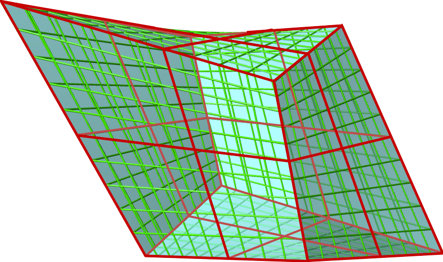
Figure 17. A Blaschke cube is a skew cube whose faces are crisscrossed skew quadrilaterals. If all crosses are internal, they determine an adapted hyperboloid patch for each face, otherwise they may be understood as adapted hyperboloids.

Lemma 22 (Blaschke cubes).

1. Let $C$ be a cube in $\mathbb{R}\textup{P}^{3}$ with skew quadrilateral faces. Furthermore, consider twelve additional points, one on each extended edge of $C$. Given five faces of $C$, if, for each face, the four points on the edges are coplanar then the four points associated with the remaining face are also coplanar. In other words, the extension of five faces to crisscrossed quadrilaterals is consistent and yields a unique cross for the sixth face.

2. The three lines connecting the centres of opposite crosses of a Blaschke cube are concurrent.

Proof.

Both claims follow directly from the description of crosses in terms of $\rho$ (cf. Lemma 18). To verify part ii), we label the vertices of the cube by $x_{1},\ldots,x_{8}$ and note that the point

$$p=\frac{\rho_{1}x_{1}+\rho_{2}x_{2}+\rho_{3}x_{3}+\rho_{4}x_{4}+\rho_{5}x_{5}+\rho_{6}x_{6}+\rho_{7}x_{7}+\rho_{8}x_{8}}{\rho_{1}+\rho_{2}+\rho_{3}+\rho_{4}+\rho_{5}+\rho_{6}+\rho_{7}+\rho_{8}}$$

is contained in each of the lines connecting opposite centres. ∎

4.1. Imposing the $C^{1}$-condition on multidimensional crisscrossed A-nets

While the previous considerations show that it is always possible to extend an A-net $x:\mathbb{Z}^{m}\to\mathbb{R}^{3}$ to a crisscrossed A-net, it is not obvious that the $C^{1}$-condition can be imposed consistently on each 2-dimensional layer of $x$. We show that this is possible by first describing the corresponding Cauchy problem algebraically in terms of $\rho$ and then giving a geometric proof for the consistency of the evolution equations.

Cauchy problem for crisscrossed A-nets that satisfy the $C^{1}$-condition in 2D coordinate planes.

If we assume that the $C^{1}$-condition holds for coordinate planes of higher-dimensional A-nets then one obtains an extension of the system (23) for A-surfaces, namely

(28) $$\rho_{iij}=\frac{\rho_{ii}\rho_{j}}{\rho a^{ij}a^{ij}_{i}},\quad i,j\in\{1,\dots,m\},\ i\neq j.$$

For a given supporting A-net, in order to be able to propagate initial values $\rho$ to all vertices of $\mathbb{Z}^{m}$ according to (28), one has to prescribe Cauchy data along the coordinate axes and a suitable unit hypercube, for instance

(29) $$\rho(\mathcal{S}^{i}),\ i=1,\dots,m;\quad\rho(\left\{0,1\right\}^{m}).$$

It remains to show that for data (29) the propagation according to (28) is consistent. The 2-dimensional compatibility conditions $(\rho_{iij})_{j}=(\rho_{ijj})_{i}$ are satisfied by virtue of Lemma 20. The elementary 3-dimensional compatibility condition is captured by

Lemma 23.

Imposition of the $C^{1}$-condition (28) on the four pairs of adjacent quadrilaterals of two neighbouring cubes of an A-net, as depicted in Fig. 18, is consistent. This means, if we start with the Cauchy data $\rho,\rho_{j},\rho_{k},\rho_{jk},\rho_{ii}$ and successively apply (28) then the compatibility conditions

(30) $$(\rho_{iij})_{k}=(\rho_{iik})_{j}$$

are satisfied so that $\rho_{iijk}$ is well defined.

Figure 18. The $C^{1}$-condition can be consistently imposed on coordinate planes of a crisscrossed A-net locally, i.e., for two face-adjacent cubes.

Remark 24.

Lemma 23 guarantees that if the $C^{1}$-condition is satisfied on three of the “compound long faces” in Fig. 18, then it is also satisfied on the remaining compound face.

Geometric proof of Lemma 23. We give a Menelaus-type proof of (30), analogous to the geometric proof of Lemma 20. In terms of the notation of Fig. 19, left, we define the multi-ratios

$$M=\frac{l(x_{1},p_{41})}{l(p_{41},x_{4})}\frac{l(x_{4},p_{34})}{l(p_{34},x_{3})}\frac{l(x_{3},p_{23})}{l(p_{23},x_{2})}\frac{l(x_{2},p_{12})}{l(p_{12},x_{1})},\quad\tilde{M}=\frac{l(\tilde{x}_{1},\tilde{p}_{12})}{l(\tilde{p}_{12},\tilde{x}_{2})}\frac{l(\tilde{x}_{2},\tilde{p}_{23})}{l(\tilde{p}_{23},\tilde{x}_{3})}\frac{l(\tilde{x}_{3},\tilde{p}_{34})}{l(\tilde{p}_{34},\tilde{x}_{4})}\frac{l(\tilde{x}_{4},\tilde{p}_{41})}{l(\tilde{p}_{41},\tilde{x}_{1})}$$

and

$$M_{ij}=\frac{l(x_{i},p_{ij})}{l(p_{ij},x_{j})}\frac{l(x_{j},s_{j})}{l(s_{j},\tilde{x}_{j})}\frac{l(\tilde{x}_{j},\tilde{p}_{ij})}{l(\tilde{p}_{ij},\tilde{x}_{i})}\frac{l(\tilde{x}_{i},r_{i})}{l(r_{i},x_{i})},\quad j=i+1\mod 4.$$

Figure 19. Combinatorial picture of two face-adjacent cubes of an A-net. Points and lines of the same colour are coplanar and bold quadrilateral faces are skew.

The generalized Menelaus Theorem (Theorem 11) implies that the condition $M=1$ is equivalent to the coplanarity of $p_{12},p_{23},p_{34},p_{41}$, and the analogous statement holds for $\tilde{M}=1$. Combining Menelaus’ theorem with Lemma 14, we see that $M_{ij}=1$ is equivalent to $p_{ij}$ and $\tilde{p}_{ij}$ being related by the $C^{1}$-condition. Assuming $M=M_{12}=M_{23}=M_{34}=M_{41}=1$, we have to show that $\tilde{M}=1$, which is done by demonstrating that

(31) $$M\tilde{M}M_{12}M_{23}M_{34}M_{41}=1.$$

In terms of the cross-ratio of four collinear points, we see that

$$M_{12}M_{23}M_{34}M_{41}=M^{-1}\tilde{M}^{-1}\prod_{i=1}^{4}\operatorname{cr}(x_{i},s_{i},\tilde{x}_{i},r_{i})$$

and (31) becomes

(32) $$\prod_{i=1}^{4}\operatorname{cr}(x_{i},s_{i},\tilde{x}_{i},r_{i})=1.$$

To verify $\eqref{eq:stacked_cubes_multiratios_identity_crrs}$, we project the lines $\operatorname{inc}[x_{i},\tilde{x}_{i}]$ onto the diagonals of the middle quadrilateral $(y_{1},y_{2},y_{3},y_{4})$ (see Fig. 18, right). Each line $\operatorname{inc}[x_{i},\tilde{x}_{i}]$ is projected through $y_{i}$ onto the diagonal $\operatorname{inc}[y_{j},y_{k}]$ that does not contain $y_{i}$. Note that $y_{i}$ and the lines $\operatorname{inc}[x_{i},\tilde{x}_{i}]$ and $\operatorname{inc}[y_{j},y_{k}]$ are coplanar due to planarity of the vertex star of $y_{i}$. One obtains (indices taken modulo 4)

(33) $$\operatorname{cr}(x_{i},s_{i},\tilde{x}_{i},r_{i})=\operatorname{cr}(z_{i},y_{i-1},\tilde{z}_{i},y_{i+1}).$$

Using $\operatorname{cr}(c,b,a,d)=\operatorname{cr}(a,b,c,d)^{-1}$ and (33), equation (32) becomes

$$\operatorname{cr}(z_{1},y_{4},\tilde{z}_{1},y_{2})\operatorname{cr}(z_{3},y_{2},\tilde{z}_{3},y_{4})=\operatorname{cr}(\tilde{z}_{2},y_{1},z_{2},y_{3})\operatorname{cr}(\tilde{z}_{4},y_{3},z_{4},y_{1})$$

$$\iff \operatorname{cr}(z_{1},y_{4},z_{3},y_{2})\operatorname{cr}(\tilde{z}_{1},y_{2},\tilde{z}_{3},y_{4})=\operatorname{cr}(y_{1},z_{4},y_{3},z_{2})\operatorname{cr}(y_{1},\tilde{z}_{2},y_{3},\tilde{z}_{4}).$$

Due to the geometry of an A-net (see Fig. 20) we have

$$\operatorname{cr}(z_{1},y_{4},z_{3},y_{2})=\operatorname{cr}(y_{1},z_{4},y_{3},z_{2}),\quad\operatorname{cr}(\tilde{z}_{1},y_{2},\tilde{z}_{3},y_{4})=\operatorname{cr}(y_{1},\tilde{z}_{2},y_{3},\tilde{z}_{4}),$$

which finally proves the claim. ∎

Figure 20. For an elementary hexahedron of a generic A-net, both the four extended edges $l_{1},\dots,l_{4}$ and the four blue diagonals are skew. Since each of those quadrupels of lines intersects the other quadrupel, they are contained in the two complementary reguli of a hyperboloid. Therefore, each quadrupel has a well-defined cross-ratio, e.g., $\operatorname{cr}(l_{1},l_{2},l_{3},l_{4})=\operatorname{cr}(p_{1},p_{2},p_{3},p_{4})=\operatorname{cr}(q_{1},q_{2},q_{3},q_{4})$.

We obtain

Proposition 25.

The $C^{1}$-condition can be imposed consistently on 2-dimensional layers of a crisscrossed A-net $(x,\rho):\mathbb{Z}^{m}\to\mathbb{R}^{3}\times\mathbb{R}$.

Proof.

Combining Lemma 20 and Remark 24, it is evident that (28) can be imposed consistently on $\mathbb{Z}^{3}$. To verify that this implies consistency in all higher dimensions, consider $z\in\mathbb{Z}^{m+1},m\geq 3$ and assume consistency on each $m$-dimensional sublattice. The point $z$ is the intersection of $m$-dimensional sublattices $Z_{1},\dots,Z_{m+1}$, with $Z_{i}\cong\mathbb{Z}^{m}$. The values of $\rho(z)$ induced by different sublattices $Z_{i}$ and $Z_{j}$ with $\dim(Z_{i}\cap Z_{j})\geq 2$ coincide, because the evolution equations (28) for $\rho$ are 2-dimensional equations. This shows that all sublattices $Z_{i}$ induce the same value for $\rho(z)$ by considering all possible pairs $Z_{i},Z_{j}$. ∎

General solution $\rho$ for a crisscrossed A-net that satisfies the $C^{1}$-condition in 2D coordinate planes.

We will now investigate in more detail those functions $\rho:\mathbb{Z}^{m}\to\mathbb{R}$ which correspond to crosses that satisfy the $C^{1}$-condition in each coordinate plane of a given A-net $x:\mathbb{Z}^{m}\to\mathbb{R}^{3},m\geq 3$. In particular, in the 3-dimensional case, we derive explicitly the general form of $\rho$ in terms of a potential $\tau$ for the Moutard coefficients associated with $x$ and demonstrate that $\rho$ satisfies a non-autonomous version of the discrete BKP equation (14). It is noted that the latter will subsequently be shown to reduce to the standard discrete BKP equation in the context of Weingarten pairs of (pre-)hyperbolic nets, leading to the remarkable relation $\rho=\tau$ (see Remark 45 and Theorem 49).

Consider the evolution equations (28) for $\rho$ satisfying the $C^{1}$-condition in coordinate planes and firstly note that these equations are invariant with respect to the change $a^{ij}\leftrightarrow a^{ji}=-a^{ij}$ of Moutard coefficients. If we fix one family of Moutard coefficients $a^{ij}$ for every $(i,j)$-coordinate plane of $\mathbb{Z}^{m}$, e.g., by the condition $i<j$, then there exist potentials $\tau:\mathbb{Z}^{m}\to\mathbb{R}$ that satisfy (12). With respect to such a potential, the system (28) may be written as

(34) $$\frac{\rho_{j}\rho_{ii}}{\rho\rho_{iij}}=a^{ij}a^{ij}_{i}=\frac{\tau_{j}\tau_{ii}}{\tau\tau_{iij}},\quad i,j\in\{1,\dots,m\},\ i\neq j.$$

If we define

(35) $$\xi=\frac{\rho}{\tau}$$

then the system (34) may be stated as

(36) $$\frac{\xi_{j}\xi_{ii}}{\xi\xi_{iij}}=1,\quad i,j\in\{1,\dots,m\},\ i\neq j$$

and introduction of the quantities

(37) $$q^{ij}=q^{ji}=\frac{\xi_{i}\xi_{j}}{\xi\xi_{ij}},\quad i,j\in\{1,\dots,m\},\ i\neq j$$

transforms the system (36) into

(38) $$q^{ij}q^{ij}_{i}=1,\quad i,j\in\{1,\dots,m\},\ i\neq j.$$

The solutions $q^{ij}$ of (38) may be expressed in terms of $\xi$ according to (37) if the corresponding compatibility conditions

(39) $$\frac{q^{ij}}{q^{ij}_{k}}=\frac{q^{jk}}{q^{jk}_{i}}=\frac{q^{ki}}{q^{ki}_{j}},\quad i,j,k\in\{1,\dots,m\},\ i\neq j\neq k\neq i$$

are satisfied. Thus, the general solution $\xi$ of (36) is encoded in the compatible relations (37) with the $q^{ij}$ satisfying the coupled system (38), (39).

Now, denote

$$\mathcal{C}^{k}\alpha=\alpha^{(-1)^{k}}$$

and let $z=(z_{1},\dots,z_{m})\in\mathbb{Z}^{m}$ be coordinates of $\mathbb{Z}^{m}$. The general solution of (38) is given by

(40) $$q^{ij}=\mathcal{C}^{z_{i}}\mathcal{C}^{z_{j}}\alpha^{ij}=\mathcal{C}^{z_{i}+z_{j}}\alpha^{ij},$$

where the functions $\alpha^{ij}$ are independent of $z_{i}$ and $z_{j}$ but otherwise arbitrary. In order to demonstrate how the remaining relations (39) determine the functions $\alpha^{ij}$, we here consider the case $m=3$ and merely state that an analogous procedure applies for $m>3$. In the 3-dimensional case, (40) becomes

(41) $$q^{12}=\mathcal{C}^{z_{1}+z_{2}}\alpha^{12}(z_{3}),\quad q^{23}=\mathcal{C}^{z_{2}+z_{3}}\alpha^{23}(z_{1}),\quad q^{31}=\mathcal{C}^{z_{3}+z_{1}}\alpha^{31}(z_{2})$$

and the relations (39) read

$$\frac{q^{12}}{q^{12}_{3}}=\frac{q^{23}}{q^{23}_{1}}=\frac{q^{31}}{q^{31}_{2}}.$$

Therefore,

(42) $$\mathcal{C}^{z_{1}+z_{2}}\left(\frac{\alpha^{12}}{\alpha^{12}_{3}}\right)=\mathcal{C}^{z_{2}+z_{3}}\left(\frac{\alpha^{23}}{\alpha^{23}_{1}}\right)=\mathcal{C}^{z_{3}+z_{1}}\left(\frac{\alpha^{31}}{\alpha^{31}_{2}}\right)$$

and, under the change of variables

(43) $$\alpha^{12}=\mathcal{C}^{z_{3}}\tilde{\alpha}^{12},\quad\alpha^{23}=\mathcal{C}^{z_{1}}\tilde{\alpha}^{23},\quad\alpha^{31}=\mathcal{C}^{z_{2}}\tilde{\alpha}^{31},$$

we may write (42) as

$$\mathcal{C}^{z_{1}+z_{2}+z_{3}}(\tilde{\alpha}^{12}\tilde{\alpha}^{12}_{3})=\mathcal{C}^{z_{1}+z_{2}+z_{3}}(\tilde{\alpha}^{23}\tilde{\alpha}^{23}_{1})=\mathcal{C}^{z_{1}+z_{2}+z_{3}}(\tilde{\alpha}^{31}\tilde{\alpha}^{31}_{2}).$$

Since $\tilde{\alpha}^{ij}$ is independent of $z_{i}$ and $z_{j}$, we see that

$$\tilde{\alpha}^{12}\tilde{\alpha}^{12}_{3}=\tilde{\alpha}^{23}\tilde{\alpha}^{23}_{1}=\tilde{\alpha}^{31}\tilde{\alpha}^{31}_{2}=\text{const},$$

which allows us to introduce constants $\beta^{12},\beta^{23},\beta^{31},\beta\in\mathbb{C}$, such that the $\tilde{a}^{ij}$ are given by

(44) $$\tilde{\alpha}^{12}=(\mathcal{C}^{z_{3}}(\beta^{12})^{4})\beta^{4},\quad\tilde{\alpha}^{23}=(\mathcal{C}^{z_{1}}(\beta^{23})^{4})\beta^{4},\quad\tilde{\alpha}^{31}=(\mathcal{C}^{z_{2}}(\beta^{31})^{4})\beta^{4}.$$

Combining (41), (43), and (44) yields

(45) $$\begin{split}q^{12}=\left(\mathcal{C}^{z_{1}+z_{2}}(\beta^{12})^{4}\right)\left(\mathcal{C}^{z_{1}+z_{2}+z_{3}}\beta^{4}\right),\\ q^{23}=\left(\mathcal{C}^{z_{2}+z_{3}}(\beta^{23})^{4}\right)\left(\mathcal{C}^{z_{1}+z_{2}+z_{3}}\beta^{4}\right),\\ q^{31}=\left(\mathcal{C}^{z_{3}+z_{1}}(\beta^{31})^{4}\right)\left(\mathcal{C}^{z_{1}+z_{2}+z_{3}}\beta^{4}\right).\end{split}$$

Performing the variable substitution

(46) $$\xi=\tilde{\xi}\left(\mathcal{C}^{z_{1}+z_{2}}(\beta^{12})^{-1}\right)\left(\mathcal{C}^{z_{2}+z_{3}}(\beta^{23})^{-1}\right)\left(\mathcal{C}^{z_{3}+z_{1}}(\beta^{31})^{-1}\right)\left(\mathcal{C}^{z_{1}+z_{2}+z_{3}}\beta^{-1}\right),$$

relations (37) become

$$q^{ij}=\frac{\xi_{i}\xi_{j}}{\xi\xi_{ij}}=\frac{\tilde{\xi}_{i}\tilde{\xi}_{j}}{\tilde{\xi}\tilde{\xi}_{ij}}\left(\mathcal{C}^{z_{i}+z_{j}}(\beta^{ij})^{4}\right)\left(\mathcal{C}^{z_{1}+z_{2}+z_{3}}\beta^{4}\right)$$

so that (45) implies that

(47) $$\frac{\tilde{\xi}_{i}\tilde{\xi}_{j}}{\tilde{\xi}\tilde{\xi}_{ij}}=1.$$

The general solution $\tilde{\xi}$ of (47) is given by

(48) $$\tilde{\xi}(z)=f^{(1)}(z_{1})f^{(2)}(z_{2})f^{(3)}(z_{3}),\quad f^{({i})}:\mathbb{Z}\to\mathbb{C}^{*}.$$

Combination of equations (35), (46), (48) yields the general solution $\rho$ of (34) in terms of $\tau$, namely

(49) $$\rho=(\mathcal{C}^{z_{1}+z_{2}}\gamma^{12})(\mathcal{C}^{z_{2}+z_{3}}\gamma^{23})(\mathcal{C}^{z_{3}+z_{1}}\gamma^{31})(\mathcal{C}^{z_{1}+z_{2}+z_{3}}\gamma)f^{(1)}(z_{1})f^{(2)}(z_{2})f^{(3)}(z_{3})\ \tau,$$

where the constants $\gamma,\gamma^{ij}\in\mathbb{C}$ and functions $f^{({i})}:\mathbb{Z}\to\mathbb{C}$ have to be chosen in such a manner that $\rho\in\mathbb{R}^{*}$ but may otherwise be arbitrary.

Remark 26.

Equation (11) for Moutard coefficients expressed in terms of a potential $\tau$ that satisfies (12) becomes a discrete BKP (dBKP) equation

(50) $$\tau\tau_{123}+\varepsilon^{1}\tau_{1}\tau_{23}+\varepsilon^{2}\tau_{2}\tau_{13}+\varepsilon^{3}\tau_{3}\tau_{12}=0$$

with $\varepsilon^{i}=\pm 1$ depending on which Moutard coefficients are chosen to be parametrized by $\tau$. Accordingly, $\rho$ defined by (49) satisfies the corresponding (integrable) non-autonomous BKP-type equation

(51) $$\rho\rho_{123}+\kappa^{1}\rho_{1}\rho_{23}+\kappa^{2}\rho_{2}\rho_{13}+\kappa^{3}\rho_{3}\rho_{12}=0,$$

where

$$\kappa^{1}=\varepsilon^{1}(\mathcal{C}^{z_{1}+z_{2}}\gamma^{12})^{4}(\mathcal{C}^{z_{3}+z_{1}}\gamma^{31})^{4},$$

$$\kappa^{2}=\varepsilon^{2}(\mathcal{C}^{z_{1}+z_{2}}\gamma^{12})^{4}(\mathcal{C}^{z_{2}+z_{3}}\gamma^{23})^{4},$$

$$\kappa^{3}=\varepsilon^{3}(\mathcal{C}^{z_{2}+z_{3}}\gamma^{23})^{4}(\mathcal{C}^{z_{3}+z_{1}}\gamma^{31})^{4}.$$

Remark 27.

Given a potential $\tau$ that parametrizes a certain choice of Moutard coefficients, a function $\tilde{\tau}=\tilde{\xi}\tau$ is another potential if and only if

$$\frac{\tilde{\tau}_{i}\tilde{\tau}_{j}}{\tilde{\tau}\tilde{\tau}_{ij}}=\frac{\tilde{\xi}_{i}\tilde{\xi}_{j}}{\tilde{\xi}\tilde{\xi}_{ij}}\frac{\tau_{i}\tau_{j}}{\tau\tau_{ij}}=\frac{\tau_{i}\tau_{j}}{\tau\tau_{ij}},$$

i.e., if and only if $\tilde{\xi}$ satisfies (47). Therefore, in the 3-dimensional case, the general potential $\tilde{\tau}$ which parametrizes the same Moutard coefficients as $\tau$ is given by

$$\tilde{\tau}=f^{(1)}(z_{1})f^{(2)}(z_{2})f^{(3)}(z_{3})\ \tau,$$

with $f^{(i)}:\mathbb{Z}\to\mathbb{C}^{*}$. Taking into account black-white rescaling of the Lelieuvre normals and the according rescaling of Moutard coefficients, one obtains an equivalence class of Moutard coefficients that depends only on the geometry of the underlying A-net. In terms of the potentials, any two representatives $\tau$ and $\tilde{\tau}$ of this equivalence class are related by

(52) $$\tilde{\tau}=(\mathcal{C}^{z_{1}+z_{2}+z_{3}}\gamma)f^{(1)}(z_{1})f^{(2)}(z_{2})f^{(3)}(z_{3})\ \tau$$

with $\gamma\in\mathbb{C}$ such that $\gamma^{4}\in\mathbb{R}_{+}$. Comparing (52) with (49) shows that, roughly speaking, in the 3-dimensional case and for a fixed potential $\tau$ the general solution $\rho$ of (34) may be decomposed into the general potential $\tilde{\tau}$ that parametrizes Moutard coefficients in the equivalence class of the given supporting A-net and a factor containing three additional parameters $\gamma^{12},\gamma^{23},\gamma^{31}$.

A class of canonical Bäcklund transformations for pre-hyperbolic nets.

Proposition 25 allows us to construct Bäcklund transforms of a pre-hyperbolic net $f=(x,\rho):\mathbb{Z}^{2}\to\mathbb{R}^{3}\times\mathbb{R}$ in the following sense. We start with a Weingarten transform $\tilde{x}$ of the supporting A-surface $x$. This gives a 2-layer 3D A-net $X:\mathbb{Z}^{2}\times\{0,1\}\to\mathbb{R}^{3}$, which is composed of the layers $X(\cdot,0)=x$ and $X(\cdot,1)=\tilde{x}$. The additional data needed to specify a Bäcklund transform $\tilde{f}=(\tilde{x},\tilde{\rho})$ of $f$ are the values of $\tilde{\rho}$ at the vertices of one elementary quadrilateral $\tilde{Q}$ of $\tilde{x}$ (cf. Fig. 21, left). The remaining values of $\tilde{\rho}$ are then determined by the $C^{1}$-condition imposed on vertical layers, which implies that the $C^{1}$-condition is satisfied for the resulting crisscrossed A-net $\tilde{f}$ (cf. Remark 24). Equivalently, in geometric terms, the Cauchy data needed to specify a Bäcklund transformation are cross vertices on the “vertical edges” incident to the four vertices of one elementary square $Q$ of $x$, which determines a unique Blaschke cube by virtue of Lemma 22 (cf. Fig. 21, right). Thus, we may say that a Bäcklund transform of $f$ is determined by a Weingarten transform $\tilde{x}$ of $x$ and the extension of one cube of $X$ to a Blaschke cube.

Figure 21. Left: The values of $\rho$ and $\tilde{\rho}$ at the black vertices determine the values of $\tilde{\rho}$ at the white vertices by imposing the $C^{1}$-condition on every 2-dimensional layer. Right: The black cross vertices of a Blaschke cube determine the remaining white vertices (cf. Lemma 22).

Since Cauchy data defining a Bäcklund transformation consist of the values of $\tilde{\rho}$ at the four vertices of the quadrilateral $\tilde{Q}$, the corresponding cross adapted to $\tilde{Q}$ can be chosen independently from the cross adapted to $Q$. Thus, in general, the induced hyperboloids $h$ and $\tilde{h}$ adapted to $Q$ and $\tilde{Q}$ do not form a classical Weingarten pair.

Remark 28.

Proposition 25 may be exploited to impose the $C^{1}$-condition on all coordinate surfaces of a 3-layer crisscrossed A-net $(x,\rho):\mathbb{Z}^{2}\times\left\{0,1,2\right\}\to\mathbb{R}^{3}\times\mathbb{R}$. In this case, given initial data $\rho(\mathcal{S}^{12})$ that satisfy the $C^{1}$-condition, $\rho_{33}$ already determines $\rho$ in the shifted coordinate plane $\mathcal{S}^{12}_{33}$ by means of application of the $C^{1}$-condition in all $(1,3)$- and $(2,3)$-coordinate planes. However, $\rho_{3},\rho_{13},\rho_{123},\rho_{23}$ can still be chosen independently as described above. In this way, we obtain three pre-hyperbolic nets $f^{(i)}=(x,\rho)(\cdot,i),i=0,1,2$ such that both $(f^{(0)},f^{(1)})$ and $(f^{(1)},f^{(2)})$ form a Bäcklund pair but also the nets $f^{(0)},f^{(2)}$ are related in a particular manner. Furthermore, we may apply this construction to an A-net $x$ consisting of arbitrarily many layers and construct a special sequence $f^{(0)},f^{(1)},f^{(2)},\cdots$ of Bäcklund transforms of pre-hyperbolic nets that are adapted to $x$. To this end, we choose the first Bäcklund transform $f^{(1)}$ of a given pre-hyperbolic net $f^{(0)}$ generically, while all further Bäcklund transforms are determined uniquely (up to homogeneous rescaling of $\rho$ in each “horizontal” layer) by the two initial nets. By construction, the corresponding function $\rho$ obeys the BKP-type equation (51). In this connection, it is observed that if the layers $f^{(i)}$ are merely related by Bäcklund transformations so that the $C^{1}$-condition is not necessarily satisfied on all “vertical” coordinate surfaces then the expression (49) for $\rho$ is still valid but $\gamma^{23},\gamma^{31}$ and $\gamma$ are now arbitrary functions of $z_{3}$ and $\rho$ is governed by a slight generalization of (51), which, generically, also depends on the coefficient $\gamma$.

4.2. The notion of Weingarten transformations

We begin with a characterization of crosses adapted to opposite faces of an elementary hexahedron of an A-net such that the corresponding hyperboloids form a classical Weingarten pair.

Weingarten cubes.

In the following, we use the term A-cube for an elementary hexahedron of an A-net, i.e., a cube with skew quadrilateral faces and planar vertex stars. We will show that for an A-cube with a hyperboloid $h$ adapted to one face $Q$, there exists a unique hyperboloid $\tilde{h}$ adapted to the opposite face $\tilde{Q}$, such that $h,\tilde{h}$ constitutes a Weingarten pair. In other words, there exists a unique Weingarten transformation $T$ such that $\tilde{h}=T(h)$ is a hyperboloid adapted to $\tilde{Q}$. The geometric characterization of corresponding points $y\in h$ and $\tilde{y}=T(h)\in\tilde{h}$ is that the line connecting $y$ and $\tilde{y}$ is the intersection of the tangent planes to $h$ and $\tilde{h}$ in $y$ and $\tilde{y}$ respectively. We refer to this by saying that the points $y$ and $\tilde{y}$ satisfy the Weingarten property (cf. Definition 6).

Consider an A-cube with crosses attached to opposite faces, labelled as in Fig. 22, which determine hyperboloids $h$ and $\tilde{h}$ adapted to the bottom and top faces respectively.

Figure 22. Combinatorics of an A-cube with crosses adapted to two opposite faces.

It is noted that, for any pair of adapted hyperboloids, the Weingarten property is automatically satisfied at corresponding vertices $x_{i},\tilde{x}_{i}$ due to the geometry of A-cubes, i.e., since vertex stars are planar. Now, we assume that the crosses in Fig. 22 define hyperboloids $h,\tilde{h}$, which are related by a classical Weingarten transformation $T$. Since vertices $x_{i},\tilde{x}_{i}$ are corresponding points and Weingarten transformations preserve asymptotic lines, $T$ maps the asymptotic line $\operatorname{inc}[x_{i},x_{i+1}]$ (indices taken modulo 4) of $h$ to the asymptotic line $\operatorname{inc}[\tilde{x}_{i},\tilde{x}_{i+1}]$ of $\tilde{h}$, that is,

$$T(\operatorname{inc}[x_{i},x_{i+1}])=\operatorname{inc}[\tilde{x}_{i},\tilde{x}_{i+1}].$$

In particular, each point $y\in\operatorname{inc}[x_{i},x_{i+1}]$ has a corresponding point $T(y)=\tilde{y}\in\operatorname{inc}[\tilde{x}_{i},\tilde{x}_{i+1}]$. By definition, two corresponding cross vertices $p_{ij},\tilde{p}_{ij}$ satisfy the Weingarten property if and only if

(53) $$\operatorname{inc}[p_{ij},\tilde{p}_{ij}]=\operatorname{inc}[x_{i},x_{j},p_{kl}]\cap\operatorname{inc}[\tilde{x}_{i},\tilde{x}_{j},\tilde{p}_{kl}],\quad(j,k,l)=(i+1,i+2,i+3).$$

We make the crucial observation that (53) is equivalent to each of the quadruples of points $(\tilde{p}_{ij},x_{i},x_{j},p_{kl})$ and $(p_{ij},\tilde{x}_{i},\tilde{x}_{j},\tilde{p}_{kl})$ being coplanar, i.e., pairs $(p_{ij},\tilde{p}_{kl})$ and $(\tilde{p}_{ij},p_{kl})$ of diagonally opposite cross vertices being related by the $C^{1}$-condition with respect to both of the edges $\operatorname{inc}[x_{i},x_{j}]$ and $\operatorname{inc}[\tilde{x}_{i},\tilde{x}_{j}]$ (see Lemma 14).

Without loss of generality, we may assume that $T(p_{ij})=\tilde{p}_{ij}$ for one pair of corresponding cross vertices which, in turn, implies that the opposite cross vertices $p_{kl},\tilde{p}_{kl}$ also have to satisfy $T(p_{kl})=\tilde{p}_{kl}$. This follows from the fact that Weingarten transformations preserve asymptotic lines, that is, $T(p_{ij})=\tilde{p}_{ij}$ implies $T(\operatorname{inc}[p_{ij},p_{kl}])=\operatorname{inc}[\tilde{p}_{ij},\tilde{p}_{kl}]$, and we may conclude that

$$\begin{split}T(p_{kl})&=T(\operatorname{inc}[p_{ij},p_{kl}]\cap\operatorname{inc}[x_{k},x_{l}])\\ &=T(\operatorname{inc}[p_{ij},p_{kl}])\cap T(\operatorname{inc}[x_{k},x_{l}])=\operatorname{inc}[\tilde{p}_{ij},\tilde{p}_{kl}]\cap\operatorname{inc}[\tilde{x}_{k},\tilde{x}_{l}]=\tilde{p}_{kl}.\end{split}$$

The fact that it is actually possible to have simultaneously $T(p_{ij})=\tilde{p}_{ij}$ and $T(p_{kl})=\tilde{p}_{kl}$ is due to the following important

Lemma 29 ($C^{1}$-identity).

Consider diagonally opposite cross vertices $p_{ij}$ and $\tilde{p}_{kl}$ of an A-cube equipped with crosses as in Fig. 22. The points $p_{ij},\tilde{x}_{i},\tilde{x}_{j},\tilde{p}_{kl}$ are coplanar if and only if the points $p_{ij},x_{k},x_{l},\tilde{p}_{kl}$ are coplanar.

Remark 30.

One may interpret Lemma 29 as follows: The point $\tilde{p}_{kl}$ is the projection of $p_{ij}$ through both the line $\operatorname{inc}[\tilde{x}_{i},\tilde{x}_{j}]$ and the line $\operatorname{inc}[x_{k},x_{l}]$ onto the line $\operatorname{inc}[\tilde{x}_{k},\tilde{x}_{l}]$.

Proof of Lemma 29. The most elegant geometric proof of this lemma is via Cox’ theorem (Theorem 5), applied in a suitable way [Kin]. Fig. 23, left, shows the initial A-cube, where a point and a plane are incident if they are associated with adjacent vertices. Given the crosses that are depicted in Fig. 22, the initial A-cube may be modified by replacing points $\tilde{x}_{1}$ and $x_{4}$ by $\tilde{p}_{12}\in\operatorname{inc}[\tilde{x}_{1},\tilde{x}_{2}]$ and $p_{34}\in\operatorname{inc}[x_{3},x_{4}]$, and replacing planes $P_{1}$ and $\tilde{P}_{4}$ by $E_{1}=\operatorname{inc}[p_{34},x_{1},x_{2}]$ and $\tilde{E}_{4}=\operatorname{inc}[p_{34},\tilde{x}_{3},\tilde{x}_{4}]$. According to Cox’ theorem, $\tilde{p}_{12}\in E_{1}$ if and only if $\tilde{p}_{12}\in\tilde{E}_{4}$. ∎

Figure 23. Cox deformation of an A-cube.

If we start with the A-cube in Fig 23, left and wish to make sure that the configuration in Fig. 23, right likewise constitutes an A-cube then we may choose either $\tilde{p}_{12}\in\operatorname{inc}[\tilde{x}_{1},\tilde{x}_{2}]$ or $p_{34}\in\operatorname{inc}[x_{3},x_{4}]$. Selecting, for example, $p_{34}\in\operatorname{inc}[x_{3},x_{4}]$ yields the planes $E_{1}=\operatorname{inc}[p_{34},x_{1},x_{2}]$ and $\tilde{E}_{4}=\operatorname{inc}[p_{34},\tilde{x}_{3},\tilde{x}_{4}]$. By virtue of Cox’ theorem, the points $\operatorname{inc}[\tilde{x}_{1},\tilde{x}_{2}]\cap E_{1}$ and $\operatorname{inc}[\tilde{x}_{1},\tilde{x}_{2}]\cap\tilde{E}_{4}$ coincide and define $\tilde{p}_{12}$. We refer to this construction as a Cox deformation of the original A-cube.

Remark 30 elucidates the propagation of cross vertices induced by imposition of (53). The following theorem shows that, for any given initial cross $(p_{12},p_{23},p_{34},p_{41})$, this propagation indeed yields a cross $(\tilde{p}_{12},\tilde{p}_{23},\tilde{p}_{34},\tilde{p}_{41})$ and, moreover, that the Weingarten property is satisfied for the cross centres $q$ and $\tilde{q}$. Having established this, it will be easy to demonstrate that hyperboloids given by crosses that satisfy $\eqref{eq:weingarten_property_cross_vertices}$ are indeed related by a classical Weingarten transformation (Corollary 34).

Theorem 31.

Consider an A-cube $(x_{1},\dots,x_{4},\tilde{x}_{1},\dots,\tilde{x}_{4})$ as in Fig. 22. Propagation of a cross $(p_{12},p_{23},p_{34},p_{41})$ attached to the quadrilateral $(x_{1},x_{2},x_{3},x_{4})$ according to the $C^{1}$-condition around horizontal edges (cf. Remark 30) yields a unique cross $(\tilde{p}_{12},\tilde{p}_{23},\tilde{p}_{34},\tilde{p}_{41})$ attached to the quadrilateral $(\tilde{x}_{1},\tilde{x}_{2},\tilde{x}_{3},\tilde{x}_{4})$. The centres $q$ and $\tilde{q}$ of the crosses satisfy the Weingarten property, i.e.,

(54) $$\operatorname{inc}[q,\tilde{q}]=\operatorname{inc}[p_{12},p_{23},p_{34},p_{41}]\cap\operatorname{inc}[\tilde{p}_{12},\tilde{p}_{23},\tilde{p}_{34},\tilde{p}_{41}].$$

Proof.

According to the $C^{1}$-identity (Lemma 29), propagation of the initial cross $(p_{12},p_{23},p_{34},p_{41})$ as described in Remark 30 yields four well-defined points $(\tilde{p}_{12},\tilde{p}_{23},\tilde{p}_{34},\tilde{p}_{41})$. We have to show that these points are vertices of a cross, that is, that they are coplanar.

Consider Fig. 22. In a first step, we demonstrate that the loop $(p_{12},\tilde{p}_{12},\tilde{p}_{34},p_{34})$ yields a refinement of the original A-cube $\mathcal{C}=(x_{1},\dots,x_{4},\tilde{x}_{1},\dots,\tilde{x}_{4})$ into the two smaller A-cubes $\mathcal{C}_{41}=(x_{1},p_{12},p_{34},x_{4},$ $\tilde{x}_{1},\tilde{p}_{12},\tilde{p}_{34},\tilde{x}_{4})$ and $\mathcal{C}_{23}=(x_{2},p_{12},p_{34},x_{3},\tilde{x}_{2},\tilde{p}_{12},\tilde{p}_{34},\tilde{x}_{3})$. For symmetry reasons, it is sufficient to show that $\mathcal{C}_{23}$ is an A-cube. This assertion, in turn, is true since $\mathcal{C}_{23}$ can be obtained from $\mathcal{C}$ by applying two Cox deformations as illustrated in Fig. 24.

Figure 24. Successive application of two Cox deformations.

Next, we define

$$\Pi=\operatorname{inc}[p_{12},p_{23},p_{34},p_{41}],\quad\tilde{q}=\Pi\cap\operatorname{inc}[\tilde{p}_{12},\tilde{p}_{34}],\quad\tilde{\Pi}=\operatorname{inc}[q,\tilde{p}_{12},\tilde{p}_{34}].$$

The points $p_{23}$ and $\tilde{p}_{41}$ are related by the $C^{1}$-identity with respect to the A-cube $\mathcal{C}$, i.e., $\Pi_{41}=\operatorname{inc}[p_{23},x_{1},x_{4},\tilde{p}_{41}]$ is a plane. Since $p_{41},p_{23}\in\Pi_{41}$, we also have $q\in\Pi_{41}$. This shows that $q$ and $\tilde{p}_{41}$ are related by the $C^{1}$-identity with respect to the A-cube $\mathcal{C}_{41}$. Analogously, $q$ and $\tilde{p}_{23}$ are related by the $C^{1}$-identity with respect to $\mathcal{C}_{23}$. We may state this as

$$\tilde{p}_{41}=\operatorname{inc}[\tilde{x}_{1},\tilde{x}_{4}]\cap\tilde{\Pi},\quad\tilde{p}_{23}=\operatorname{inc}[\tilde{x}_{2},\tilde{x}_{3}]\cap\tilde{\Pi},$$

which shows that

$$\tilde{\Pi}=\operatorname{inc}[\tilde{p}_{12},\tilde{p}_{23},\tilde{p}_{34},\tilde{p}_{41}].$$

In particular, the points $\tilde{p}_{12},\tilde{p}_{23},\tilde{p}_{34},\tilde{p}_{41}$ are coplanar and hence define a cross adapted to $(\tilde{x}_{1},\tilde{x}_{2},\tilde{x}_{3},\tilde{x}_{4})$. Now, we will demonstrate that, indeed,

$$\tilde{q}=\operatorname{inc}[\tilde{p}_{12},\tilde{p}_{41}]\cap\operatorname{inc}[\tilde{p}_{23},\tilde{p}_{34}],$$

i.e., $\tilde{q}$ is the centre of the top cross as suggested by Fig. 22. For now, we denote the centre of the top cross by $\tilde{c}$. We have already established that each cross determines the other cross according to (53), and that, if we propagate from bottom to top, the center of the bottom cross is contained in the plane of the top cross, that is, $q\in\tilde{\Pi}$. For symmetry reasons, we also have $\tilde{c}\in\Pi$ and, in particular,

(55) $$\operatorname{inc}[q,\tilde{c}]=\Pi\cap\tilde{\Pi}.$$

Furthermore, we define $\bar{q}=\Pi\cap\operatorname{inc}[\tilde{p}_{23},\tilde{p}_{41}]$ and assume that $\tilde{q}\neq\bar{q}$. In this case, we have three distinct points $\tilde{c},\tilde{q},\bar{q}\in\Pi$ that span the plane of the top cross, i.e., $\tilde{\Pi}=\operatorname{inc}[\tilde{c},\tilde{q},\bar{q}]$. This, in turn, implies the degenerate case $\Pi=\tilde{\Pi}$. Therefore, generically, $\tilde{q}=\bar{q}=\tilde{c}$ and (55) becomes (54). ∎

Definition 32 (Weingarten cube / Weingarten propagation of crosses).

An A-cube with two crosses adapted to opposite faces as in Fig. 22 is called a Weingarten cube if the Weingarten property (53) is satisfied by any pair $p_{ij},\tilde{p}_{ij}$ of corresponding cross vertices. According to Theorem 54, an A-cube with a cross attached to one face can be extended uniquely to a Weingarten cube by, for instance, using the projections described in Remark 30. We refer to this extension as Weingarten propagation of the initial cross.

Remark 33.

A Weingarten cube determines a unique adapted hyperboloid for each face. The data needed to extend a Weingarten cube to a Blaschke cube are one point on a “vertical” (extended) edge (see Fig. 25). This yields four crosses adapted to the vertical faces that are composed of asymptotic lines of the vertical hyperboloids.

Figure 25. Extension of a Weingarten cube to a Blaschke cube.

According to Theorem 54, it is possible to have two “$C^{1}$-loops” of crosses (or adapted hyperboloids) around an A-cube. However, it is not possible to have a third $C^{1}$-loop around the cube composed of the crosses associated with the vertical faces. The reason is that, considering three faces adjacent to one vertex, one would have the $C^{1}$-condition fulfilled around a vertex of degree 3. This would contradict the fact that interior vertices of a pre-hyperbolic net have to be of even degree. In particular, Blaschke cubes that are Weingarten cubes in multiple ways do not exist since at most one pair of opposite crosses can be related by the Weingarten property.

Finally note that, if we prescribe which pair of opposite faces has to satisfy the Weingarten property, a single hyperboloid of a Weingarten cube uniquely determines all other hyperboloids according to the $C^{1}$-condition.

Corollary 34.

Hyperboloids corresponding to crosses of a Weingarten cube form a (classical) Weingarten pair. In particular, the cross centres $q$ and $\tilde{q}$ are corresponding points.

Proof.

A cube with crosses attached to two opposite faces, top and bottom as in Fig. 22, determines hyperboloids $h,\tilde{h}$ adapted to those faces, and four hyperboloids adapted to vertical faces. If the crosses describe a Weingarten cube then any of the six adapted hyperboloids determines the remaining ones uniquely (cf. Remark 33). Any point $q\in h$ is the centre of a unique cross $c\subset h$ which determines, following asymptotic lines of the vertical hyperboloids, a unique corresponding cross $\tilde{c}\subset\tilde{h}$ with centre $\tilde{q}$. On noting that $c$ and $\tilde{c}$ are related by the Weingarten propagation, the claim follows directly from (54). ∎

It is evident that if both crosses of a Weingarten cube are internal then Corollary 34 remains valid if one replaces “hyperboloids” by “hyperboloid patches”. Hence, the preceding analysis suggests regarding a Weingarten pair of (pre-)hyperbolic nets as being composed of Weingarten cubes.

Definition 35 (Weingarten transformation).

Two (pre-)hyperbolic nets $f=(x,\rho)$ and $\tilde{f}=(\tilde{x},\tilde{\rho})$ are said to be related by a Weingarten transformation if

1. the supporting A-nets $x$ and $\tilde{x}$ form a (discrete) Weingarten pair, and

2. crosses adapted to corresponding quadrilaterals $Q$ and $\tilde{Q}$ of $x$ and $\tilde{x}$ are related by the Weingarten propagation, i.e., $Q$ and $\tilde{Q}$ equipped with these crosses are opposite faces of a Weingarten cube (see Definition 32) so that the corresponding hyperboloids (patches) form a classical Weingarten pair.

The nets $f$ and $\tilde{f}$ are said to form a Weingarten pair and $\tilde{f}$ is called a Weingarten transform of $f$.

Relation between Bäcklund and Weingarten transformations of pre-hyperbolic nets.

Even though Definition 35 is meaningful locally, a priori, it is not evident that it is possible for all cubes to be simultaneously of Weingarten type. While the analysis of Weingarten pairs of hyperbolic nets is more involved, the existence of Weingarten pairs of pre-hyperbolic nets is easily established based on the Bäcklund transformation introduced in the preceding. Here, the key is

Proposition 36.

Let $(x,\rho)$ and $(\tilde{x},\tilde{\rho})$ be a Bäcklund pair of pre-hyperbolic nets. If one cube with opposite faces $Q,\tilde{Q}$ as depicted in Fig. 21 is a Weingarten cube, then $(x,\rho)$ and $(\tilde{x},\tilde{\rho})$ form a Weingarten pair. Conversely, if $(x,\rho)$ and $(\tilde{x},\tilde{\rho})$ form a Weingarten pair then $(\tilde{x},\tilde{\rho})$ and $(x,\rho)$ are Bäcklund-related.

Proposition 36 follows almost immediately from the observation captured in the following

Lemma 37.

In the sense of Fig. 26, the $C^{1}$-condition is transitive for crisscrossed quadrilaterals that share an edge.

Figure 26. Crisscrossed quadrilaterals sharing an edge. If hyperboloids adapted to $Q_{1}$ and $Q_{2}$ are tangent along the extended edge $e$ and the same holds for $Q_{2}$ and $Q_{3}$ then the hyperboloids adapted to $Q_{1}$ and $Q_{3}$ are likewise tangent along $e$. In particular, the four cross vertices $p,p_{1},p_{2},p_{3}$ are coplanar.

Remark 38.

Lemma 37 shows that Lemma 23 is a direct consequence of Theorem 54. Furthermore, iterative application of the Weingarten transformation leads to nets for which the $C^{1}$-condition is satisfied in all coordinate planes. Thus, in the case of Weingarten transformations, Remark 28 becomes obsolete.

Remark 39.

It is not difficult to check, e.g., by considering parallel invariants, that equi-twist is transitive in the same sense as the $C^{1}$-condition.

Proof of Proposition 36. Consider adjacent cubes of a Bäcklund pair $(x,\rho),(\tilde{x},\tilde{\rho})$ as depicted in Fig. 27 and denote the constituent quadrilaterals by

$$(x_{1},x_{2},x_{5},x_{6})\leftrightarrow Q_{1256},\quad(x_{2},x_{5},\tilde{x}_{5},\tilde{x}_{2})\leftrightarrow Q_{25\tilde{5}\tilde{2}},\quad\text{etc.}$$

Figure 27. Adjacent cubes of a Bäcklund pair of pre-hyperbolic nets.

The values of $\rho$ and $\tilde{\rho}$ at the 12 vertices yield a unique cross for each of the 11 elementary quadrilaterals. Assuming that the left cube with crosses adapted to opposite faces $Q_{1256}$ and $Q_{\tilde{1}\tilde{2}\tilde{5}\tilde{6}}$ is a Weingarten cube, we now show that the right cube is a Weingarten cube as well. According to Lemma 29, it is sufficient to show that for each pair $(Q_{2345},Q_{25\tilde{5}\tilde{2}})$, $(Q_{2345},Q_{23\tilde{3}\tilde{2}})$, $(Q_{\tilde{2}\tilde{3}\tilde{4}\tilde{5}}$, $Q_{25\tilde{5}\tilde{2}})$, and $(Q_{\tilde{2}\tilde{3}\tilde{4}\tilde{5}}$, $Q_{23\tilde{3}\tilde{2}})$ of quadrilaterals the corresponding crosses satisfy the $C^{1}$-condition. For symmetry reasons, we have to consider only the two pairs containing, for example, the quadrilateral $Q_{\tilde{2}\tilde{3}\tilde{4}\tilde{5}}$. By assumption, the crosses attached to $Q_{\tilde{1}\tilde{2}\tilde{5}\tilde{6}}$ and $Q_{\tilde{2}\tilde{3}\tilde{4}\tilde{5}}$ satisfy the $C^{1}$-condition. Since the left cube is a Weingarten cube, also the crosses attached to $Q_{\tilde{1}\tilde{2}\tilde{5}\tilde{6}}$ and $Q_{25\tilde{5}\tilde{2}}$ satisfy the $C^{1}$-condition. Therefore, Lemma 37 implies that the same holds for the crosses attached to $Q_{\tilde{2}\tilde{3}\tilde{4}\tilde{5}}$ and $Q_{25\tilde{5}\tilde{2}}$. On the other hand, the pairs of crosses adapted to $(Q_{12\tilde{2}\tilde{1}},Q_{\tilde{1}\tilde{2}\tilde{5}\tilde{6}})$, $(Q_{12\tilde{2}\tilde{1}},Q_{23\tilde{3}\tilde{2}})$, and $(Q_{\tilde{1}\tilde{2}\tilde{5}\tilde{6}},Q_{\tilde{2}\tilde{3}\tilde{4}\tilde{5}})$ each satisfy the $C^{1}$-condition. Thus, according to Lemma 20, also the crosses attached to $Q_{\tilde{2}\tilde{3}\tilde{4}\tilde{5}}$ and $Q_{23\tilde{3}\tilde{2}}$ satisfy the $C^{1}$-condition. Reversing the above argument shows that, indeed, every Weingarten pair of pre-hyperbolic nets constitutes a Bäcklund pair. ∎

Proposition 36 shows that Weingarten pairs of pre-hyperbolic nets exist since Cauchy data $\tilde{\rho}$ at one initial quadrilateral $\tilde{Q}$ for a Bäcklund transformation as depicted in Fig. 21 can be chosen in such a manner that the initial cube constitutes a Weingarten cube. We obtain the following constructive description of Weingarten transformations of pre-hyperbolic nets.

Theorem 40.

Let $f=(x,\rho):\mathbb{Z}^{2}\to\mathbb{R}^{3}\times\mathbb{R}$ be a pre-hyperbolic net and let $\tilde{x}$ be a Weingarten transform of the A-surface $x$. The extension of $\tilde{x}$ to a crisscrossed A-net $\tilde{f}=(\tilde{x},\tilde{\rho})$ according to Definition 35, ii), i.e., extending elementary hexahedra to Weingarten cubes, yields a Weingarten transform $\tilde{f}$ of $f$. The Weingarten transform $\tilde{f}$ is uniquely determined (modulo homogeneous rescaling of $\tilde{\rho}$) by its supporting A-surface $\tilde{x}$.

Remark 41.

Proposition 36 states that the property of Blaschke cubes being Weingarten cubes propagates “horizontally” in a crisscrossed 2-layer 3D A-net whose two layers form a Bäcklund pair. Moreover, Weingarten cubes propagate also “vertically” in the following sense. Consider a 3D crisscrossed A-net $(x,\rho)$ that satisfies the $C^{1}$-condition in coordinate planes, i.e., $\rho$ is of the form (49) and satisfies (51). Then, any of the three families of “parallel” crisscrossed coordinate surfaces may be interpreted as a family $f^{(i)}=(x^{(i)},\rho^{(i)})$ of pre-hyperbolic nets such that for all $i$, $f^{(i)}$ and $f^{(i+1)}$ form a Bäcklund pair and, in addition, $f^{(i)},f^{(i+2)}$ are related in a particular manner (in contrast to an arbitrary family of Bäcklund transforms (c.f. Remark 28)). Now, if we assume that a single elementary cube of $(x,\rho)$ constitutes a Weingarten cube then one of the three families of Bäcklund transformations is privileged (cf. Remark 33) and the proof of Proposition 36 (the transitivity of the $C^{1}$-condition) reveals that, in fact, with respect to this distinguished family, all Bäcklund pairs represent Weingarten pairs. In this connection, we observe that even if we do not make the assumption of an initial Weingarten cube then a (weaker) Weingarten connection still exists. Thus, since for any family $f^{(i)}$ of Bäcklund transforms as defined above the $C^{1}$-condition maps the layer $f^{(i)}$ uniquely and independently of $f^{(i+1)}$ to the layer $f^{(i+2)}$ and a double application of the Weingarten transformation implies the vertical $C^{1}$ property, one may interpret $f^{(i+2)}$ as being generated from $f^{(i)}$ by a double Weingarten transformation.

Algebraic description of Weingarten pairs in terms of potentials $\tau$ that parametrize Moutard coefficients of the underlying A-net: A geometric interpretation of solutions of the dBKP equation.

Consider a supporting 2-layer 3D A-net $x:\mathbb{Z}^{2}\times\left\{0,1\right\}\to\mathbb{R}^{3}$. With respect to a potential $\tau$ for Moutard coefficients of $x$, relation (49) is the general parametrization of $\rho:\mathbb{Z}^{2}\times\left\{0,1\right\}\to\mathbb{R}^{3}$ such that $(x,\rho)$ is a Bäcklund pair of pre-hyperbolic nets adapted to the supporting A-net $x$. By virtue of Proposition 36, if, for a given $\rho:\mathbb{Z}^{2}\times\left\{0\right\}\to\mathbb{R}$ which describes the extension of $x(\cdot,0)$ to a pre-hyperbolic net, one chooses the parameters $\gamma,\gamma^{ij},f^{(i)}$ in (49) with $\gamma^{23},\gamma^{31}$ and $\gamma$ interpreted as functions of $z_{3}$ as indicated in Remark 28 such that one initial cube of $(x,\rho)$ becomes a Weingarten cube then $(x,\rho)$ describes a Weingarten pair. It turns out that this reduces (49) to $\rho=\tau$ modulo a reparametrization of $\tau$ which corresponds to black-white rescaling of Lelieuvre normals $n$ for $x$, possibly combined with a change of Moutard coefficients to be parametrized by $\tau$. The following lemma encapsulates this relation for a single Weingarten cube.

Lemma 42.

Consider a crisscrossed A-cube given by $(x,\rho)$ as in Fig. 28, left and let $n$ be Lelieuvre normals of $x$ with Moutard coefficients $a^{ij}$ chosen as in Fig. 28, middle. The pair $(x,\rho)$ governs a Weingarten cube with respect to the top and bottom faces if and only if there exists a $\lambda\in\mathbb{R}$ such that

(56) $$a^{ij}=\lambda\frac{\rho_{i}\rho_{j}}{\rho\rho_{ij}},\quad a^{ij}_{k}=\lambda^{-1}\frac{\rho_{ik}\rho_{jk}}{\rho_{k}\rho_{ijk}},\quad(i,j,k)\in\left\{(2,1,3),(2,3,1),(3,1,2)\right\}.$$

In particular, modulo a suitable black-white rescaling of $n$, either the Moutard coefficients $(a^{21},a^{23},a^{31})$ or $(a^{12},a^{32},a^{13})$ and their respective shifts are parametrized by $\rho$.

Figure 28. Algebraic data of a crisscrossed A-cube.

Proof.

We consider the two pairs of adjacent Moutard coefficients in Fig. 28, right associated with horizontal edges of direction 1 and the two corresponding pairs associated with direction 2. According to Lemma 19 / Remark 17, the Weingarten propagation of the cross determined by $(\rho,\rho_{1},\rho_{12},\rho_{2})$ is described by the conditions

(57) $$\frac{a^{31}}{a^{21}}=\frac{\rho_{3}\rho_{12}}{\rho_{2}\rho_{13}},\quad a^{21}a^{31}_{2}=\frac{\rho_{1}\rho_{23}}{\rho\rho_{123}},\quad\frac{a^{23}}{a^{21}}=\frac{\rho_{3}\rho_{12}}{\rho_{1}\rho_{23}},\quad a^{21}a^{23}_{1}=\frac{\rho_{2}\rho_{13}}{\rho\rho_{123}}.$$

Now, we define $\lambda$ such that

$$a^{21}=\lambda\frac{\rho_{1}\rho_{2}}{\rho\rho_{12}}$$

so that the relations (57) become

$$a^{23}=\lambda\frac{\rho_{2}\rho_{3}}{\rho\rho_{23}},\quad a^{31}=\lambda\frac{\rho_{1}\rho_{3}}{\rho\rho_{13}},\quad a^{23}_{1}=\lambda^{-1}\frac{\rho_{12}\rho_{13}}{\rho_{1}\rho_{123}},\quad a^{31}_{2}=\lambda^{-1}\frac{\rho_{12}\rho_{23}}{\rho_{2}\rho_{123}}.$$

Furthemore, the relation (13), i.e., equality of the three ratios of opposite Moutard coefficients, yields

$$a^{21}_{3}=\frac{a^{21}a^{23}_{1}}{a^{23}}=\frac{a^{21}a^{31}_{2}}{a^{31}}=\lambda^{-1}\frac{\rho_{13}\rho_{23}}{\rho_{3}\rho_{123}}.$$

Finally, we observe that a black-white rescaling (4) of $n$ by $\alpha$ at even vertices and by $\alpha^{-1}$ at odd vertices amounts to a rescaling of $a^{21},a^{23},a^{31}$ by $\alpha^{2}$ and a rescaling of $a^{21}_{3},a^{23}_{1},a^{31}_{2}$ by $\alpha^{-2}$. Therefore, $\lambda=\pm 1$ can always be achieved. After this normalization, either the Moutard coefficients $(a^{21},a^{23},a^{31})$ or $(a^{12},a^{32},a^{13})$ and their respective shifts are parametrized by $\rho$, depending on the sign of $\lambda$. ∎

Remark 43.

The proof of Lemma 42 demonstrates the consistency of (57) regarded as evolution equations for given $\rho,\rho_{1},\rho_{2},\rho_{3},\rho_{12}$ and represents an algebraic proof of Theorem 54.

Application of Lemma 42 to a 2-layer lattice now yields

Theorem 44.

A crisscrossed A-net $(x,\rho):\mathbb{Z}^{2}\times\left\{0,1\right\}\to\mathbb{R}^{3}\times\mathbb{R}$ encodes a Weingarten pair of pre-hyperbolic nets if and only if there exists a Lelieuvre normal field $n$ of $x$ such that $\tau=\rho$ parametrizes in the sense of (12) either the Moutard coefficients $(a^{21},a^{23},a^{31})$ or $(a^{12},a^{32},a^{13})$.

Proof.

If $\tau=\rho$ is a potential for Moutard coefficients then, according to Lemma 42, every elementary cube constitutes a Weingarten cube, i.e., $(x,\rho)$ describes a Weingarten pair. Conversely, we observe that it is possible to achieve

(58) $$\frac{\rho_{1}\rho_{2}}{\rho\rho_{12}}=\varepsilon a^{21},\quad\varepsilon=\pm 1$$

for one initial quadrilateral by applying a suitable black-white rescaling of Lelieuvre normals $n$ of $x$. With respect to this normalization,

$$\tau(\mathcal{S}^{1})=\rho(\mathcal{S}^{1}),\quad\tau(\mathcal{S}^{2})=\rho(\mathcal{S}^{2}),\quad\tau(1,1,0)=\rho(1,1,0),\quad\tau(0,0,1)=\rho(0,0,1)$$

are Cauchy data for a potential $\tau$ that parametrizes the coefficients $\varepsilon(a^{21},a^{23},a^{31})$, whereby $\varepsilon=-1$ corresponds to a parametrization of $(a^{12},a^{32},a^{13})$. With respect to this unique potential $\tau$, the $C^{1}$-condition (34) in the coordinate plane $\mathbb{Z}^{2}\times\left\{0\right\}$ reduces to $\tau(\mathcal{S}^{12})=\rho(\mathcal{S}^{12})$, which is satisfied by assumption. Now, since $\tau(0,0,1)=\rho(0,0,1)$, the Weingarten conditions (57) imply that $\tau=\rho$ on the entire cube containing the initial quadrilateral. Iterative application of this argument shows that $\tau=\rho$ everywhere. ∎

Remark 45.

If we iterate the Weingarten transformation of a pre-hyperbolic net adapted to one $(1,2)$-layer of a 3D A-net $x:\mathbb{Z}^{3}\to\mathbb{R}^{3}$ then we obtain a crisscrossed A-net $(x,\rho)$ and the above theorem implies that $\tau=\rho$ parametrizes either Moutard coefficients $(a^{21},a^{23},a^{31})$ or $(a^{12},a^{32},a^{13})$ of a distinguished Lelieuvre representation $n$ of $x$. Therefore, $\tau$ satisfies the discrete BKP equation in the form

(59) $$\tau\tau_{123}-\tau_{1}\tau_{23}-\tau_{2}\tau_{13}+\tau_{3}\tau_{12}=0$$

which characterizes potentials $\tau$ for solutions $\varepsilon(a^{21},a^{23},a^{31}),\varepsilon=\pm 1$ of (11) and constitutes the analogue of equation (14) characterizing potentials for lexicographically ordered coefficients. Conversely, if $\tau$ is a solution of (59) then the discrete Moutard equations (10) together with the discrete Lelieuvre formulae (9) give rise to a class of corresponding A-nets $x$ with Lelieuvre normals for which either the Moutard coefficients $(a^{21},a^{23},a^{31})$ or $(a^{12},a^{32},a^{13})$ are parametrized by $\tau$ and $(x,\tau)$ completely encodes a family of Weingarten pairs of pre-hyperbolic nets with respect to the distinguished $(1,2)$-coordinate planes. In this manner, a novel geometric intepretation of the discrete BKP equation (59) is uncovered in that the solution of the latter directly parametrizes the hyperboloids (patches) adapted to a corresponding A-net. In general, solutions of discrete BKP equations of the type (14) with two plus and two minus signs on a 3-dimensional lattice correspond to families of Weingarten transforms with respect to the associated distinguished $(i,k)$-coordinate planes.

4.3. Equi-twisted 3D A-nets and Weingarten transformations of hyperbolic nets

A pre-hyperbolic net $(x,\rho)$ is a hyperbolic net if all crosses are internal and therefore describe hyperboloid patches. This is the case if and only if $\rho$ is strictly positive or strictly negative. Assuming that an A-surface $x$ is simply connected, it is possible to extend $x$ to a hyperbolic net if and only if $x$ is equi-twisted, i.e., if and only if all parallel invariants of $x$ are positive (cf. Proposition 21).

The key aspect in the determination of Weingarten transformations of hyperbolic nets is the analysis of the equi-twist properties of multidimensional A-nets. In Theorem 40, it is justified to replace the term “pre-hyperbolic net” by “hyperbolic net” if we can ensure that all 3-dimensional A-cubes have the property that the Weingarten propagation of crosses preserves internal crosses. We begin with the discussion of cubes that have this property.

Definition 46 (Equi-twisted A-cubes).

We call an A-cube equi-twisted with respect to a pair $(Q,\tilde{Q})$ of opposite faces if both loops of edge-adjacent quadrilaterals containing $Q$ and $\tilde{Q}$ are equi-twisted.

Lemma 47.

Let $\mathcal{C}$ be an A-cube with an internal cross attached to one face $Q$. The Weingarten propagation of this cross to the opposite face $\tilde{Q}$ yields an internal cross adapted to $\tilde{Q}$ if and only if $\mathcal{C}$ is equi-twisted with respect to $(Q,\tilde{Q})$.

Proof.

Propagation of cross vertices according to the $C^{1}$-condition maps an internal vertex to an internal vertex if and only if the corresponding two edge-adjacent quadrilaterals are equi-twisted (Lemma 19). This implies that two edge-adjacent quadrilaterals of an A-cube are equi-twisted if and only if the opposite two quadrilaterals are equi-twisted (cf. Remark 30) and the claim of the lemma follows (cf. Fig. 29). ∎

Figure 29. An internal cross vertex $p$ is propagated to an internal cross vertex $\tilde{p}$ if and only if $(Q,Q_{r})$ are equi-twisted, which is equivalent to $(Q_{l},\tilde{Q})$ being equi-twisted. If both, $(Q,Q_{l})$ and $(Q,Q_{r})$ are equi-twisted then the complete loop $(Q,Q_{r},\tilde{Q},Q_{l})$ is equi-twisted.

Equi-twisted A-cubes exist in the following sense. We recall the algebraic description (57) of the Weingarten propagation in the context of Fig. 28 and observe, in analogy with Lemma 19, that an internal cross adapted to the bottom quadrilateral of the cube in Fig. 28, left is propagated to an internal cross adapted to the top quadrilateral if and only if the four relevant parallel invariants are positive, i.e.,

(60) $$\frac{a^{31}}{a^{21}}>0,\quad a^{21}a^{31}_{2}>0,\quad\frac{a^{23}}{a^{21}}>0,\quad a^{21}a^{23}_{1}>0.$$

This means that the cube in question is equi-twisted with respect to the top and bottom quadrilaterals if and only if (60) is satisfied and, hence, we have to demonstrate that it is possible to achieve (60) for a single A-cube. In terms of arbitrarily chosen Moutard coefficients $a^{21},a^{23},a^{31}$, the propagation (11) of those coefficients on an A-cube reads

(61) $$a^{ij}_{k}=\frac{a^{ij}}{a^{21}(a^{23}+a^{31})-a^{23}a^{31}}.$$

Now, it is possible to choose positive coefficients $a^{21},a^{23},a^{31}$ in such a manner that the denominator in (61) is positive so that a solution of (60) is obtained. It is noted that the coefficient $a^{21}_{3}$ is then also positive, which corresponds to the symmetry of equi-twisted A-cubes with respect to the two distinguished opposite faces. Fig. 30 displays an example of an equi-twisted Weingarten cube and the associated hyperboloid patches.

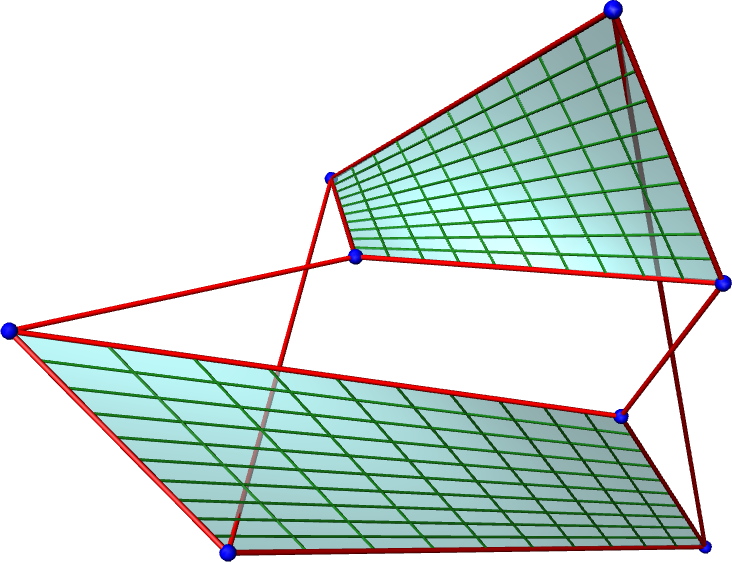
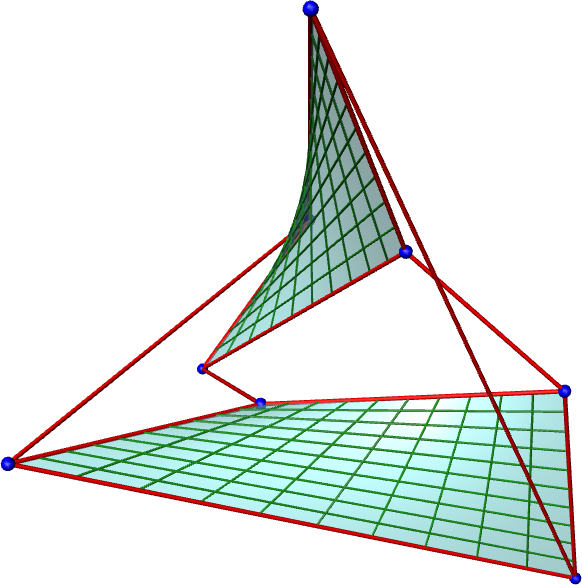
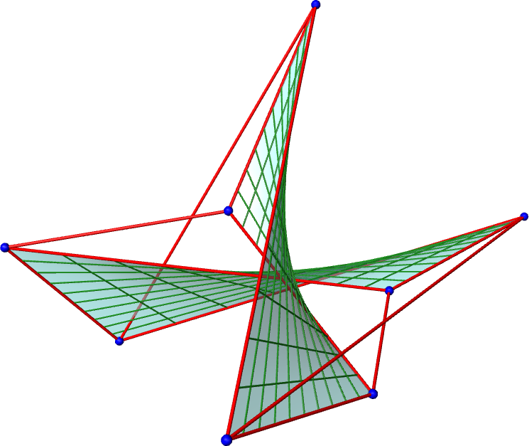
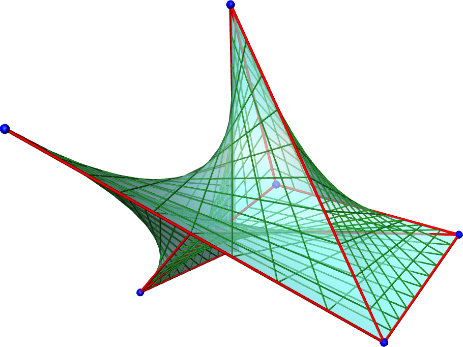
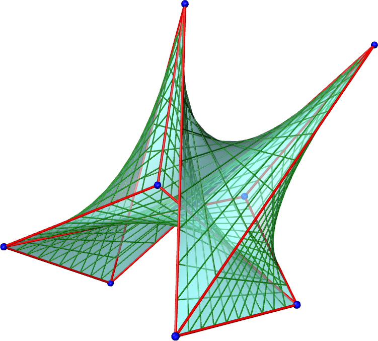
Figure 30. Top: An equi-twisted A-cube with a Weingarten pair of hyperboloid patches adapted to opposite faces. Bottom: The same cube completed with the unique patches that are adapted to vertical faces and determined by the distinguished Weingarten pair via the $C^{1}$-condition.

Remark 48.

The previous considerations show that it is impossible for all three loops of an A-cube to be equi-twisted. Indeed, the equi-twist conditions associated with the additional ”horizontal” loop of quadrilaterals in Fig. 28 may be expressed as $a^{31}/a^{23}<0$ and $a^{31}a^{23}_{1}<0$, which cannot be satisfied simultaneously with (60). An analogous argument may be used to show that all interior vertices of an equi-twisted A-surface are of even degree.

Based on Definition 46, we say that an A-net $x:\mathbb{Z}^{3}\to\mathbb{R}^{3}$ is equi-twisted with respect to consecutive layers $x^{(k)}=x(\cdot,k)$ and $x^{(k+1)}=x(\cdot,k+1)$ if the elementary hexahedra ”between” the restrictions of $x$ to $x^{(k)}$ and $x^{(k+1)}$ are equi-twisted with respect to corresponding opposite quadrilaterals of $x^{(k)}$ and $x^{(k+1)}$. As a consequence, each of the layers $x^{(k)},x^{(k+1)}$ is then equi-twisted itself (see Remark 39). Thus, by virtue of Lemma 47, the Weingarten propagation of (internal crosses of) a hyperbolic net adapted to $x^{(k)}$ generates a Weingarten transform adapted to $x^{(k+1)}$ if and only if $x$ is equi-twisted with respect to $x^{(k)},x^{(k+1)}$. The previous considerations, in particular, the algebraic equi-twist condition (60), combined with Theorem 44 and Remark 45 lead to the following description of equi-twisted A-nets and Weingarten transformations of adapted hyperbolic nets.

Theorem 49.

1. A-nets $x:\mathbb{Z}^{3}\to\mathbb{R}^{3}$ that are equi-twisted with respect to any two consecutive $(1,2)$-layers are characterized by the property that, for any Lelieuvre representation, either the Moutard coefficients $(a^{21},a^{23},a^{31})$ or $(a^{12},a^{32},a^{13})$ may be parametrized by positive solutions $\tau$ of the discrete BKP equation (59).

2. Hyperbolic nets that are adapted to the (1,2)-layers of an A-net $x:\mathbb{Z}^{3}\to\mathbb{R}^{3}$ and represented as $(x,\rho):\mathbb{Z}^{3}\to\mathbb{R}^{3}\times\mathbb{R}$ constitute a family of Weingarten transforms if and only if there exists a Lelieuvre normal field $n$ of $x$ such that $\tau=\rho$ parametrizes according to (12) either the Moutard coefficients $(a^{21},a^{23},a^{31})$ or $(a^{12},a^{32},a^{13})$ of $n$.

3. In particular, if $\tau$ is a positve solution of (59) and $x$ is an A-net with Moutard coefficients $(a^{21},a^{23},a^{31})$ or $(a^{12},a^{32},a^{13})$ parametrized by $\tau$ then $(x,\tau)$ encapsulates a family of Weingarten pairs of hyperbolic nets with respect to the $(1,2)$-coordinate planes.

Remark 50.

The trivial solution $\tau\equiv 1$ of (59) corresponds to Weingarten transformations of the affine minimal surfaces analysed in [CAL10, KP13] since $\tau_{1}\tau_{2}/\tau\tau_{12}=\rho_{1}\rho_{2}/\rho\rho_{12}=1$ corresponds to hyperbolic paraboloid patches adapted to (1,2)-quadrilaterals (cf. Remark 13).

We conclude with the following statement about general Weingarten pairs of hyperbolic nets.

Proposition 51.

The class of Weingarten pairs of hyperbolic nets may be parametrized in terms of one-dimensional Cauchy data and a function of two variables (encoding one of the two hyperbolic A-nets) which is locally bounded below.

Proof.

According to Theorem 49, the analysis of Weingarten pairs of hyperbolic nets is equivalent to the analysis of A-nets $x:\mathbb{Z}^{2}\times\left\{0,1\right\}\to\mathbb{R}^{3}$ that are equi-twisted with respect to the two layers denoted by $x^{(0)}=x(\cdot,0)$ and $x^{(1)}=x(\cdot,1)$. A necessary and sufficient condition for $x$ being equi-twisted with respect to $x^{(0)},x^{(1)}$ is that for every elementary hexahedron the corresponding Moutard coefficients satisfy (60). Therefore, it is sufficient to confine ourselves to the consideration of Moutard coefficients and related Cauchy problems. If we think of $x^{(0)}$ as a given equi-twisted layer then it is convenient to regard the relevant Moutard coefficients as functions of the “horizontal” variables $z_{1}$ and $z_{2}$, that is,

(62) $$a^{23},a^{31},a,a_{3}:\mathbb{Z}^{2}\to\mathbb{R}^{3},$$

where $a:=a^{21}$. Hence, since $x^{(0)}$ is equi-twisted, we may assume without loss of generality that $a>0$. It is therefore required to show that (60) holds for all A-cubes “between” the two layers $x^{(0)}$ and $x^{(1)}$, that is,

(63) $$a_{3},a^{23},a^{31}>0.$$

The latter Moutard coefficients are determined by the evolution equations (61) with Cauchy data consisting of coefficients $a$ for quadrilaterals of the $(1,2)$-plane and $a^{23},a^{31}$ for the “vertical” quadrilaterals over the coordinate axes of the $(1,2)$-plane, i.e.,

(64) $$a(\mathcal{S}^{12}),\quad a^{23}(\left\{0\right\}\times\mathbb{Z}),\quad a^{31}(\mathbb{Z}\times\{0\}).$$

As a necessary condition, the above Cauchy data have to be chosen positive.

In order to proceed, we now cast the Cauchy problem into a form which reflects the privileged role of the $(1,2)$-coordinate planes. Thus, the relation

$$\frac{a^{23}}{a^{23}_{1}}=\frac{a^{31}}{a^{31}_{2}},$$

which is a consequence of (61), guarantees the existence of a potential $\Phi$ such that

(65) $$a^{23}=\frac{\Phi}{\Phi_{2}},\quad a^{31}=\frac{\Phi}{\Phi_{1}}.$$

With respect to this potential, the evolution equations (61) may then be written as

(66) $$\Phi_{12}=a(\Phi_{1}+\Phi_{2})-\Phi,\quad a_{3}=\frac{\Phi_{1}\Phi_{2}}{\Phi\Phi_{12}}a.$$

Accordingly, in terms of $\Phi$, the Cauchy data (64) translate into the Cauchy data

$$a(\mathcal{S}^{12}),\quad\Phi(\left\{0\right\}\times\mathbb{Z}),\quad\Phi(\mathbb{Z}\times\left\{0\right\}).$$

The parametrization (65) now shows that the positivity of the Moutard coefficients $a^{23}$ and $a^{31}$ leads to the key condition

$$\Phi>0.$$

The latter is satisfied if the Cauchy data $\Phi(\left\{0\right\}\times\mathbb{Z})$ and $\Phi(\mathbb{Z}\times\left\{0\right\})$ are positive and, at each step of the iteration, the Moutard coefficient $a$ in the four-point equation (66)₁ is chosen in such a way that

(67) $$a>\frac{\Phi}{\Phi_{1}+\Phi_{2}}.$$

Finally, relation (66)₂ shows that the positivity of $\Phi$ implies the positivity of the remaining coefficient $a_{3}$. ∎

Remark 52.

In broad terms, if, in the context of the above proof, we regard the A-surface $x^{(0)}$ as a discretization of a continuous surface then the condition (67) imposes a constraint on the “quality” of the discretization of any particular surface rather than the surface itself. More precisely, in the context of the continuum limit alluded to in Section 2.1, the functions $a$ and $\Phi$ admit the expansions

$$a=1+\frac{1}{2}\varepsilon_{1}\varepsilon_{2}A+\cdots,\quad\Phi_{1}=\Phi+\varepsilon_{1}\partial_{1}\Phi+\cdots,\quad\Phi_{2}=\Phi+\varepsilon_{2}\partial_{2}\Phi+\cdots$$

and the discrete Moutard equation (66)₁ formally reduces to the classical Moutard equation

$$\partial_{1}\partial_{2}\Phi=A\Phi$$

in the limit $\varepsilon_{i}\to 0$. The inequality (67) then adopts the form

$$1+\varepsilon_{1}\frac{\partial_{1}\Phi}{\Phi}+\varepsilon_{2}\frac{\partial_{2}\Phi}{\Phi}+\varepsilon_{1}\varepsilon_{2}A+\cdots>0$$

which may be met for sufficiently “small” discretization parameters $\varepsilon_{i}$ subject to appropriate boundedness assumptions on the functions $A$ and $\Phi$.

5. Perspectives

The preceding analysis has revealed that Weingarten transformations for hyperbolic nets are algebraically encoded in positive solutions of the discrete BKP equation (59). A single application of a Weingarten transformation corresponds to a positive solution $\tau:\mathbb{Z}^{2}\times\{0,1\}\to\mathbb{R}$ of the discrete BKP equation and the existence of such solutions has been proven in Proposition 51. Iterated Weingarten transformations for hyperbolic nets correspond to positive solutions $\tau$ of the discrete BKP equation which are defined on larger domains. In which sense these exist in both geometric and algebraic terms is currently being investigated. In this context, it is also natural to examine the permutability theorems associated with Weingarten transformations. Furthermore, it is necessary to inquire as to whether the positivity of $\tau$ may be preserved by the standard Bäcklund transformation for the discrete BKP equation. In geometric terms, this is closely related to the consideration of four- or higher-dimensional dimensional hyperbolic nets. In this connection, the application of Weingarten transformations to special discrete surfaces such as the discrete K-surfaces alluded to in the Introduction should be pursued. All these items will be addressed in a separate publication.

References

- [BB38] W. Blaschke and G. Bol, Geometrie der Gewebe. Topologische Fragen der Differentialgeometrie., (Die Grundlehren d. math. Wiss. in Einzeldarstell. mit besonderer Berücksichtigung der Anwendungsgebiete. 49) Berlin: Julius Springer. VIII, 339 S., 137 Fig. , 1938 (German).
- [BHV12] A.I. Bobenko and E. Huhnen-Venedey, Curvature line parametrized surfaces and orthogonal coordinate systems: discretization with dupin cyclides, Geometriae Dedicata 159 (2012), no. 1, 207–237.
- [BP96] A.I. Bobenko and U. Pinkall, Discrete surfaces with constant negative Gaussian curvature and the Hirota equation., J. Differ. Geom. 43 (1996), no. 3, 527–611 (English).
- [BS99a] A.I. Bobenko and W.K. Schief, Affine spheres: Discretization via duality relations., Exp. Math. 8 (1999), no. 3, 261–280 (English).
- [BS99b] by same author, Discrete indefinite affine spheres., Bobenko, Alexander I. (ed.) et al., Discrete integrable geometry and physics. Based on the conference on condensed matter physics and discrete geometry, Vienna, Austria, February 1996. Oxford: Clarendon Press. Oxf. Lect. Ser. Math. Appl. 16, 113-138 (1999)., 1999.
- [BS08] A.I. Bobenko and Yu.B. Suris, Discrete Differential Geometry. Integrable structure., Graduate Studies in Mathematics, vol. 98, AMS, 2008.
- [CAL10] M. Craizer, H. Anciaux, and T. Lewiner, Discrete affine minimal surfaces with indefinite metric, Differential Geom. Appl. 28 (2010), no. 2, 158–169.
- [DNS01] A. Doliwa, M. Nieszporski, and P.M. Santini, Asymptotic lattices and their integrable reductions. I: The Bianchi-Ernst and the Fubini-Ragazzi lattices., J. Phys. A, Math. Gen. 34 (2001), no. 48, 10423–10439 (English).
- [Dol01] A. Doliwa, Discrete asymptotic nets and -congruences in Plücker line geometry, J. Geom. Phys. 39 (2001), no. 1, 9–29. MR 1827693 (2002k:53016)
- [Eis60] L.P. Eisenhart, A Treatise on the Differential Geometry of Curves and Surfaces, Dover, New York, 1960.
- [Hir77] R. Hirota, Nonlinear partial difference equations. III. Discrete sine-Gordon equation, J. Phys. Soc. Japan 43 (1977), no. 6, 2079–2086. MR 0460936 (57 #925c)
- [Hof99] T. Hoffmann, Discrete Amsler surfaces and a discrete Painlevé III equation., Bobenko, Alexander I. (ed.) et al., Discrete integrable geometry and physics. Based on the conference on condensed matter physics and discrete geometry, Vienna, Austria, February 1996. Oxford: Clarendon Press. Oxf. Lect. Ser. Math. Appl. 16, 83-96 (1999)., 1999.
- [HVR13] E. Huhnen-Venedey and T. Rörig, Discretization of asymptotic line parametrizations using hyperboloid surface patches, Geometriae Dedicata (2013), 1–25 (English).
- [Kin] A.D. King, private communication.
- [KP00] B.G. Konopelchenko and U. Pinkall, Projective generalizations of Lelieuvre’s formula., Geom. Dedicata 79 (2000), no. 1, 81–99 (English).
- [KP13] F. Käferböck and H. Pottmann, Smooth surfaces from bilinear patches: discrete affine minimal surfaces, Comput. Aided Geom. Design (2013), to appear.
- [Miw82] T. Miwa, On Hirota difference equations, Proc. Japan Acad. 58 (1982), 9–12.
- [Nie02] M. Nieszporski, On a discretization of asymptotic nets., J. Geom. Phys. 40 (2002), no. 3-4, 259–276 (English).
- [NS97] J.J.C. Nimmo and W.K. Schief, Superposition principles associated with the Moutard transformation: An integrable discretization of a -dimensional sine-Gordon system., Proc. R. Soc. Lond., Ser. A 453 (1997), no. 1957, 255–279 (English).
- [RS02] C. Rogers and W.K. Schief, Bäcklund and Darboux transformations. Geometry and modern applications in soliton theory., Cambridge Texts in Applied Mathematics. Cambridge: Cambridge University Press. xvii, 413 p., 2002 (English).
- [Sau37] R. Sauer, Projektive Liniengeometrie., 194 S. Berlin, W. de Gruyter & Co. (Göschens Lehrbücherei I. Gruppe, Bd. 23) , 1937.
- [Sau50] by same author, Parallelogrammgitter als Modelle pseudosphärischer Flächen., Math. Z. 52 (1950), 611–622 (German).
- [SWP13] L. Shi, J. Wang, and H. Pottmann, Smooth surfaces from rational bilinear patches, Preprint, 2013.
- [Wun51] W. Wunderlich, Zur Differenzengeometrie der Flächen konstanter negativer Krümmung, Österreich. Akad. Wiss. Math.-Nat. Kl. S.-B. IIa. 160 (1951), 39–77. MR 0056342 (15,60g)