21 cm Angular Spectrum of Cosmic String Loops

Abstract

The 21 cm signatures induced by moving cosmic string loops are investigated. Moving cosmic string loops seed filamentary nonlinear objects. We analytically evaluate the differential 21 cm brightness temperature from these objects. We show that the brightness temperature reaches $200$ mK for a loop whose tension is about the current upper limit, $G\mu\sim 10^{-7}$. We also calculate the angular power spectrum, assuming scaling in loop distribution. We find that the angular power spectrum for $G\mu>10^{-8}$ at $z=30$ or $G\mu>10^{-10}$ at $z=20$ can dominate the spectrum of the primordial density fluctuations. Finally we show that a future SKA-like observation has the potential to detect the power spectrum due to loops with $G\mu=10^{-8}$ at $z=20$.

I Introduction

Cosmic strings are topological defects that could be produced at phase transitions in the early universe Kibble:1976sj (for reviews, see Refs. VilenkinBook ; Hindmarsh:1994re ). Therefore, a detection or a constraint of cosmic strings can give us direct access to high energy particle physics and the early universe.

Cosmic strings can produce various observational phenomena, such as CMB anisotropies Kaiser:1984iv ; Seljak:1997ii ; Allen:1997ag ; Albrecht:1997nt ; Pogosian:2004ny ; Bevis:2007qz ; Bevis:2007gh ; Pogosian:2007gi ; Fraisse:2007nu ; Hindmarsh:2009es ; Hindmarsh:2009qk ; Regan:2009hv ; Dvorkin:2011aj ; Ringeval:2012tk ; Ade:2013xla , CMB spectral distortions Tashiro:2012pp ; Chu:2013fqa , early large scale structure formations Zeldovich:1980gh ; Vilenkin:1981iu ; Silk:1984xk ; 1986MNRAS.222P..27R ; Hara:1993ga , early reionization Avelino:2003nn ; Pogosian:2004mi ; Olum:2006at ; Shlaer:2012rj and gravitational waves Vachaspati:1984gt ; Damour:2000wa ; Damour:2001bk ; Damour:2004kw ; Olmez:2010bi ; vanHaasteren:2011ni ; Sanidas:2012ee ; Binetruy:2012ze . Since most observational effects due to strings are gravitational, we can set observational constraints on the strength of gravitational interactions of strings which is parametrized by the dimensionless number $G\mu$, where $G$ is Newton’s constant and $\mu$ is the mass per unit length (or tension) of string. The current limit on $G\mu$ is obtained from CMB anisotropy observations. WMAP and SPT data provide the limit $G\mu<1.7\times 10^{-7}$ Dvorkin:2011aj . Recently Planck data updated the limit to $G\mu<1.5\times 10^{-7}$ Ade:2013xla .

Cosmological 21 cm observation is expected as one of the new observational windows for cosmic strings. Since the intensity of the redshifted 21 cm lines of neutral hydrogen is sensitive to the number density and temperature of neutral hydrogen, cosmological 21 cm observation has the potential to probe the high redshift Universe through the epoch of reionization ($8<z<20$) to the dark ages ($z>20$) (for reviews, see Refs. Furlanetto:2006jb ; Pritchard:2011xb ). Additionally, choosing the observational frequency, we can obtain the three-dimensional map of the redshifted 21 cm intensity 1997ApJ…475..429M . Therefore, cosmological 21 cm observation is suitable for searching the signatures of the structure formations due to cosmic strings. Currently, there are some ongoing and future projects for measuring the cosmological 21 cm radiation; MWA, LOFAR, GMRT, PAPER, SKA and Omniscope Tegmark:2009kv .

Cosmological 21 cm signatures due to cosmic strings have been investigated in several papers Khatri:2008zw ; Berndsen:2010xc ; Brandenberger:2010hn ; Hernandez:2011ym ; Hernandez:2012qs . It is well-known that a cosmic string produces overdense regions by inducing gravitational collapse of baryons onto the string wake. Moreover, if the tension of the cosmic string exceeds a critical value, the collapsed gas is heated by the collapse shock. As a result, the cosmic wake can produce strong signature in redshifted 21 cm maps, even if the tension of the string is smaller than the current constraint, $G\mu\sim 10^{-7}$ Brandenberger:2010hn ; Hernandez:2012qs . The angular 21 cm power spectrum due to string wakes has also been investigated in Ref. Hernandez:2011ym .

In this paper, we study cosmological redshifted 21 cm signature and its angular power spectrum due to cosmic string loops. Loops are produced through self-interactions and intercommunications of long strings. Since loops can create gravitational fields, they serve as seeds for nonlinear structures. The 21 cm signature due to a static loop have been studied in Ref. Pagano:2012cx . A loop induces a spherical gravitational collapse of matter and produces a bright spot on a redshifted 21 cm map. The brightness temperature of the spot reaches 1 K for $G\mu\sim 10^{-7}$. However loops are expected to have relativistic initial velocity when they are produced Vachaspati:1984dz ; Allen:1990tv . The non-zero initial velocity makes the collapsed object have a filamentary structure. Compared with the spherical collapse case due to a static loop, the density contrast inside the object is small, and the resultant shock heating at the collapse is not efficient. However the signature is elongated on a map. We compute the gas temperature in the filament due to a moving loop and evaluate the 21 cm signature. We also calculate the angular power spectrum, assuming scaling in loop distribution Vanchurin06 ; Ringeval07 ; Olum07 .

This paper is organized as follows. In Sec. II, we briefly review the the accretion onto a moving loop. In Sec. III, we investigate the differential brightness temperature of redshifted 21 cm lines induced by a loop. In Sec. IV, assuming the loop number density distribution, we evaluate the angular 21 cm power spectrum. We show the angular power spectrum for different values of $G\mu$ and redshifts. We conclude in Sec. V. Throughout this paper, we use natural units ($\hbar=c=1$), and assume $\Lambda$CDM cosmology with $\Omega_{M}=0.26$, $\Omega_{B}=0.05$ and $h=0.7$, which are consistent with the WMAP 9-year results Hinshaw:2012aka .

II accretion onto a moving loop

A loop can become a seed of structure formations. Matter accretes onto a loop, following the gravitational field due to the loop. In this section, we briefly review the evolution of the structure produced by a loop (for details, see Ref. VilenkinBook ).

First we assume that a loop is formed at time $t_{i}$ with length $L=\alpha t_{i}$ and an initial velocity $v_{i}$. Since loops are non-relativistic objects, their velocity evolution is given by

$$v(t,t_{i})=v_{i}{a_{i}\over a(t)},$$ (1)

where $a(t)$ is the scale factor and the subscript $i$ denotes the value at $t_{i}$. Throughout this paper, we take the values, $\alpha=0.1$ and $v_{i}=0.3$, suggested by simulations BlancoPillado:2011dq . The matter accretion occurs in the matter dominated era, while, in the radiation dominated era, the accretion is prevented because of the radiation pressure. Therefore, the mater accretion starts at time

$$t_{s}(t_{i})=\left\{\begin{array}[]{cc}t_{{\rm eq}},\quad{\rm for}\quad t_{i}<t_{{\rm eq}}\\ t_{i},{~{}}\quad{\rm for}\quad t_{i}>t_{{\rm eq}}\end{array}\right.,$$ (2)

where $t_{{\rm eq}}$ is the time of matter-radiation equality.

When the loop length $L$ is smaller than the horizon scale, the gravitational field due to the loop at time $t$ is described as the field due to the point mass with mass $\mu L$ and velocity $v(t,t_{i})$. Accordingly the accretion is axially symmetric along the direction of the velocity, and the resultant overdense structure is like a filament. The comoving length of the filament structure, $l_{l}$, corresponds to the comoving length of the loop trajectory after $t_{s}$,

$$l_{l}(t,t_{i})=3{v_{s}t_{s}\over a_{s}}\left(1-\sqrt{a_{s}\over a(t)}\right),$$ (3)

where the subscript $s$ denotes the value at $t_{s}$. In Fig. 1, we plot the dependence of $l_{l}$ on the initial redshift $z_{i}=z(t_{i})$ at which a loop with length $\alpha t_{i}$ is produced. As the redshift $z_{i}$ increases, the length of the filament $l_{l}$ decreases. In particular, the length $l_{l}$ is strongly suppressed for loops which are produced at $z_{i}>z_{\rm eq}$, because such loops do not have large velocities at time $t_{s}$, where matter accretion starts.

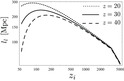
Figure 1: The comoving length of the filament $l_{l}$ as a function of the redshift $z_{i}$ corresponding to the time $t_{i}$ at which loops with $L=\alpha t_{i}$ are formed. The dotted, solid and dashed lines represent $l_{l}$ at $z=20$, $z=30$ and $z=40$, respectively.

The accretion evolution on a loop with the initial velocity has been studied by using the Zel’dovich approximation in the cylindrical coordinates $(r,\phi,l)$, where the $l$–axis corresponds to the direction of the velocity. The turnaround surface $r_{\rm t}$ on the $r$–axis is obtained by solving the equation where $r_{\rm t}$ appears on both sides Bertschinger (1987),

$$r_{\rm t}=2d(t_{i})f(t,t_{i})g_{r}(r_{\rm t},t_{i},l).$$ (4)

Here

$$d(t_{i})={3v_{s}t_{s}},\quad f(t,t_{i})={1\over 5}{G\mu L\over v_{s}^{2}d(t_{i})}{a(t)\over a_{s}},\quad g_{r}(r,t_{i},l)={R_{f}-R_{i}\over r}+{ld(t_{i})\over rR_{i}},$$ (5)

where $R_{i}=(r^{2}+l^{2})^{1/2}$ and $R_{f}=[r^{2}+(l-d(t_{i}))^{2}]^{1/2}$. For our region of interest of $(t,t_{i})$, $f(t,t_{i})$ is much less than one. In this limit, the solution of Eq. (4) is given by an approximated analytic form,

$$r_{\rm t}(t,t_{i},l)=\sqrt{4f(t,t_{i})d(t_{i})(d(t_{i})-l)}/a_{s}.$$ (6)

Fig. 2 shows the dependence of $r_{\rm t}$ on $z_{i}$. As the universe evolves, the turnaround surface becomes large. In Eq. (6), $G\mu$ dependence appears only in $f(t,t_{i})$. Therefore $r_{\rm t}$ is proportional to $\sqrt{G\mu}$. The resultant filament structure is very elongated because

$${l_{l}(t,t_{i})\over r_{\rm t}(t,t_{i})}\sim 1000\left({G\mu\over 10^{-8}}\right)^{-1/2}\quad{\rm at\ }t(z=30).$$ (7)

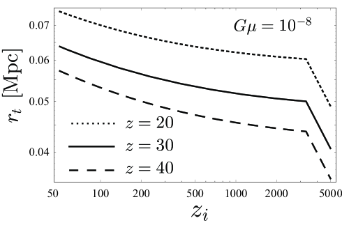
Figure 2: The comoving turnaround surface of the filament $r_{\rm t}$ as a function of the redshift $z_{i}$. In this figure, we set $G\mu=10^{-8}$ and $l=l_{l}/2$. The dotted, solid and dashed lines represent $r_{\rm t}$ at $z=20$, $z=30$ and $z=40$, respectively. The turnaround surface $r_{\rm t}$ is proportional to $\sqrt{G\mu}$.

The accreted mass at time $t$ corresponds to the mass inside $r_{\rm t}(t)$ along the trajectory $l_{l}(t)$ in the comoving frame,

$$M(t,t_{i})\approx\rho_{M}\int_{0}^{d}\pi r_{\rm t}(t)^{2}dl={3\over 5}\mu L{a(t)\over a_{s}},$$ (8)

where $\rho_{M}$ is the comoving matter density. Eq. (8) tells us that the accreted mass is proportional to $G\mu$. We plot the accreted mass in Fig. 3. The accreted mass grows as the universe evolves. Since the mass depends on the loop length $L$, the mass is proportional to $z_{i}^{3/2}$. However, since the loop generated before $z_{\rm eq}$ cannot produce the filament until $z_{\rm eq}$, the resultant filament mass is suppressed for $z>z_{\rm eq}$.

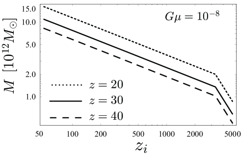
Figure 3: The filament mass dependence on $z_{i}$. In this figure, we set $G\mu=10^{-8}$. The dotted, solid and dashed lines represent the filament mass at $z=20$, $z=30$ and $z=40$, respectively. The mass of the filament is proportional to $G\mu$.

The gas inside the turnaround surface $r_{\rm t}$ collapses and is virialized. The collapsed object shrinks to about half of the physical turnaround surface scale. Although dark matter condenses in the center of the object, baryon suffers the virialization shock due to the collapse. As a result, the baryon distribution is almost homogeneous and isothermal at the virial temperature. The virial temperature of the filament structure is given by Eisenstein:1996pr

$$T_{\rm vir}\approx{1\over 2}m_{p}G\lambda_{\rm fil}.$$ (9)

Here $m_{p}$ is the proton mass and $\lambda_{\rm fil}$ is a linear mass density of the filament structure,

$$\lambda_{\rm fil}\sim{M(t,t_{i})\over a(t)l_{l}(t,t_{i})},$$ (10)

where $a(t)l_{l}(t,t_{i})$ represents the physical length scale of the filament. Since $M$ is proportional to $G\mu$ and $l_{l}$ does not depend on $G\mu$, $T_{\rm vir}$ is proportional to $G\mu$. We plot the evolution of the virial temperature of the filament in Fig. 4.

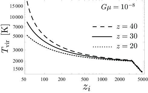
Figure 4: The virial temperature of the filament as a function of the redshift $z_{i}$ In this figure, we set $G\mu=10^{-8}$. The dashed, solid and dotted lines represent $T_{\rm vir}$ at $z=40$, $z=30$ and $z=20$, respectively. The virial temperature is proportional to $G\mu$.

We assume that the virialized radius is half of the physical turnaround surface scale. Accordingly, the matter density contrast inside the filament is

$$\rho_{f}={4\rho_{M}},$$ (11)

where $\rho_{M}$ is the background matter density. Although the turnaround surface depends on $l$ as shown Eq. (6), for simplicity, we introduce the typical turnaround surface $\bar{r}_{\rm t}$ which corresponds the turnaround surface at $l=l_{l}/2$.

III 21 cm signature from the accreted filament

As shown in the previous section, the gas density and temperature inside a filament are different from those of background values. This difference makes the optical depth of the 21 cm transition in the filament different from one in the intergalactic medium (IGM). As a result, we can observe the filament due to the loop in the differential brightness temperature map of the redshifted 21 cm line.

The optical depth of a filament to the photon at the frequency $\nu$ along the Line Of Sight (LOS) is calculated as the one of a virialized object Furlanetto:2002ng ,

$$\tau(\nu)={3A_{10}\over 32\pi k\nu_{*}^{2}}\int dR~{}{x_{\rm HI}(R)n_{H}(R)\over T_{s}(R)}\phi(\nu),$$ (12)

where $\nu_{*}$ is the hyperfine transition frequency, $\nu_{*}=1420.4~{}$MHz, $A_{10}=2.85\times 10^{-15}{\rm s}^{-1}$ is the spontaneous emission rate, $x_{\rm HI}$ is the neutral fraction of hydrogen, $T_{s}$ is the spin parameter, and $\phi(\nu)$ is the intrinsic line profile.

Now we focus on the filament whose virial temperature is smaller than $10^{4}~{}$K. When the virial temperature exceeds $10^{4}~{}$K, the atomic cooling is efficient enough to cause the further collapse and the star formations occur in the filament structure. Once stars form, they ionize the surrounding hydrogen by emitting UV photons. However, below $10^{4}~{}$K, no sources of UV photons are produced inside. Therefore, we set the neutral fraction $x_{\rm HI}=1$ inside the filament.

The spin temperature is related to the ratio between the neutral hydrogen number density in the excited and ground states of the hyperfine structure. Without stars, the excitation or de-excitation of the hyperfine structure is caused by the thermal kinetic collision at the virial temperature, the spontaneous emission and the stimulated emission by CMB photons. Therefore the spin temperature of the filament is obtained as Field (1958, 1959)

$$T_{s}={T_{\gamma}+y_{k}T_{\rm vir}\over 1+y_{k}}.$$ (13)

Here $y_{k}$ is the kinematic coupling term Kuhlen:2005cm ,

$$y_{k}={T_{*}n_{\rm Hf}\kappa\over A_{10}T_{\rm vir}},$$ (14)

where $T_{*}=0.068~{}$K, $\kappa$ is the effective single-atom rate coefficient; $\kappa=3.1\times 10^{-11}T^{0.357}\exp(-32/T){\rm cm}^{3}{\rm s}^{-1}$, and $n_{\rm Hf}$ is the neutral hydrogen number density of the filament, $n_{\rm Hf}=\rho_{f}\Omega_{B}/(m_{p}\Omega_{M})$.

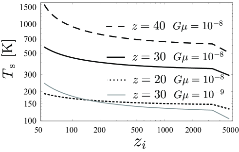
Figure 5: The spin temperature of the filament as a function of $z_{i}$. The dashed, solid and dotted lines represent $T_{s}$ at $z=40$, $z=30$ and $z=20$ with $G\mu=10^{-8}$, respectively. We also plot $T_{s}$ at $z=30$ with $G\mu=10^{-9}$ as the gray line.

The integration in Eq. (12) is performed along the LOS. Since our filament model is isothermal and has the uniform density profile, the integration can be replaced by the column density of the filament along the LOS. As discussed in the previous section, the loop with length $L$ produces the filament whose comoving typical radius is $(1/2)\bar{r}_{\rm t}$. We define the impact parameter $b$ from the symmetrical axis in the unit of $(1/2)\bar{r}_{\rm t}$. The width of the filament along the LOS depends on the impact parameter and the angle between the LOS direction and the symmetrical axis of the filament, $\psi$. Therefore, the column hydrogen number density of the filament at redshift $z$ with the impact parameter $b$ is written as

$$N_{\rm H}(b)=n_{Hf}{a\bar{r}_{\rm t}\over\sin\psi}\sqrt{1-{b^{2}\over a^{2}}},$$ (15)

where $a$ is the scale factor at $z$. Note that, since the filament has the finite length, the column number density cannot exceed $an_{Hf}l_{l}$. Therefore we set this upper limit on the column number density.

With the column hydrogen number density, the optical depth of the filament to the photon at the frequency $\nu$ along the LOS with the impact parameter $b=0$ and $\sin\psi=1$ is given by

$$\tau_{0}(\nu)={3A_{10}\over 32\pi\nu_{*}^{2}}{N_{\rm H}(0)\over k_{B}T_{s}}\phi(\nu).$$ (16)

The intrinsic line profile is broadened by the Doppler effect, because the gas inside the filament has high temperature. We adopt the Doppler broadened form,

$$\phi_{D}(\nu)=(\Delta\nu\sqrt{\pi})^{-1}\exp\left[-(\nu-\nu_{*})^{2}/\Delta\nu^{2}\right],$$ (17)

with $\Delta\nu=\nu_{*}\sqrt{2k_{B}T_{\rm vir}/m_{\rm H}}$. The Hubble flow also causes the line broadening as considered in Ref. Pagano:2012cx . The redshift difference along the LOS is given as $\delta\nu=2Hax_{t}/\sin\psi$. As a result, the intrinsic line profile broadened by the Hubble flow is Pagano:2012cx

$$\phi_{H}(\nu)=\left\{\begin{array}[]{ll}1/\delta\nu&|\nu-\nu_{*}|<\delta\nu/2\\ 0&{\rm otherwise}\\ \end{array}\right..$$ (18)

We take into account only the largest effect between them. In most of our cases, the Doppler effect dominates the Hubble flow effect.

The observable quantity is the differential brightness temperature of the 21 cm signal. In the case with $\tau\ll 1$, the differential brightness temperature of the filament with $b=0$ and $\sin\psi=1$ at $z$ is given by

$$\delta T_{b0}(\nu_{\rm obs})={T_{s}-T_{\gamma}(z)\over 1+z}\tau_{0}(\nu_{\rm obs}(1+z)),$$ (19)

where $\nu_{\rm obs}$ is the observation frequency; $\nu_{\rm obs}=(1+z)\nu_{*}$. We plot the brightness temperature $\delta T_{b0}$ in Fig. 6.

The loops produced from $z\sim 100$ to $1000$ can create the signal $\delta T_{b0}\sim 150$ mK around $z=30$. As $G\mu$ increases, the signal becomes stronger. Although the filaments due to large loops have larger spin temperature, their differential brightness temperature $\delta T_{b0}$ is strongly damped. Since such filaments have large virial temperature, the Doppler broadening is effective enough to suppress $\delta T_{b0}$.

It is worth pointing out that our values are smaller than the ones in Ref. Pagano:2012cx in which a loop produces the brightness temperature as high as 1 K for $G\mu\sim 10^{-7}$. This is because they have considered static loops. Static loops produce spherical collapsed objects. The density contrast in such objects is roughly 64, while the one in the filament object is 4. Therefore, a static loop can produce larger signal than a moving loop.

According to Eq. (19), the sign of $\delta T_{b0}$ depends on the difference between $T_{s}$ and $T_{\gamma}$. As shown in Fig. 5, most of the filaments due to loops with $G\mu=10^{-8}$ have spin temperature larger than the CMB temperature. Therefore, the 21 cm signals from such filaments are observed as emissions for the CMB, namely $\delta T_{b0}>0$. On the other hand, the loops with $G\mu=10^{-9}$ produce filaments whose spin temperature is lower than $T_{s}$ for $G\mu=10^{-8}$. In particular, the spin temperature of the filaments produced by small loops generated before $z_{\rm eq}$ is strongly suppressed. As a result, the spin temperature becomes smaller than the CMB temperature, and the signal of the filaments which have such lower temperatures are observed as absorptions for the CMB.

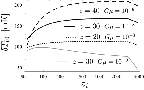
Figure 6: The brightness temperature of the filament $\delta T_{b0}$ as a function of $z_{i}$. The dashed, solid and dotted lines represent $\delta T_{b0}$ at $z=40$, $z=30$ and $z=20$ with $G\mu=10^{-8}$, respectively. We also plot $\delta T_{b0}$ at $z=30$ with $G\mu=10^{-9}$ as the gray line.

Following Eq. (15), we can extend Eq. (19) to the differential brightness temperature with the impact parameter $b$ and the angle $\psi$,

$$\delta T_{b}(\nu_{\rm obs},b,\psi)={\delta T_{b0}(\nu_{\rm obs})\over\sin\psi}\sqrt{1-{b^{2}\over a^{2}}}.$$ (20)

Since filaments due to loops have non-zero differential brightness temperature, the filaments are observable by 21 cm observations. We can observe the filament as a projection on the 2-D angular map of the celestial sphere. The projected filament with the angle $\psi$ of the LOS at the redshift $z$ is a rectangle with the angular scales of the sides, $\theta_{x}=r_{t}/(2D_{A})$ and $\theta_{y}=l_{l}\sin\psi/D_{A}$ where $D_{A}$ is the comoving angular diameter distance to $z$. For the redshift $z=30$, $\theta_{x}$ corresponds to $\sim 1^{\prime\prime}$. The angular resolution of the current design of the planned cosmological 21 cm observations is much larger than this angle scale. Therefore, it is difficult to resolve an individual filament due to a loop by the 21 cm observations.

However filaments can contribute to the angular power spectrum on the observable scales of the 21 cm observations as the tail of the angular power spectrum of the filaments on large scales. In the next section, we evaluate the angular power spectrum of the 21 cm signals from the filaments due to loops.

IV angular power spectrum

In order to calculate the angular power spectrum of 21 cm signals from the filaments due to loops, we follow the analytical approach to calculate the the Sunyaev–Zel’dovich effect due to large-scale filament structures shimon:2012vs . The total angular power spectrum due to nonlinear structures can be separated into two parts 1988MNRAS.233..637C . The first component is a Poisson term which is the contribution from the correlation between two points in the same structure. The second is a clustering term due to the correlations between different structures. We assume that the spatial distribution of loops is totally random, and there is no correlations between different filaments. Therefore, the angular power spectrum due to loops can be expressed only by the Poisson term,

$$C_{\ell}=\int dz{dV(z)\over dz}\int dL\int d\psi{dn(L,z)\over dL}f(\psi)W(\nu_{\rm obs},z)^{2}P({\ell},L,\psi),$$ (21)

where $V(z)$ is a comoving volume element per steradian at a redshift $z$, ${dn(L,z)/dL}$ is the comoving number density per unit length of loops of length $L$ at $z$, $f(\psi)$ is the probability function for the angle between the LOS and the symmetrical axis of the filament, $\psi$, and $P({\ell},L,\psi)$ is the 2-dimensional power spectrum of the 21 cm signal from a single filament produced by a loop of length $L$ and angle $\psi$, which we shall discuss later. In Eq. (21), $W(\nu_{\rm obs},z)$ is a response function associated with bandwidth of the experiment. Generally, $W(\nu_{\rm obs},z)$ is a function of the frequency centered at the observed frequency $\nu_{\rm obs}$. Since there is one to one correspondence between the frequency and the redshift, the response function $W(\nu_{\rm obs},z)$ has a peak at the redshift $z$ which satisfies $\nu_{\rm obs}=\nu_{*}/(1+z)$. For simplicity, we take $W(\nu_{\rm obs},z)$ to be flat with the width $\Delta z=1$ in redshift space. We set $f(\psi)=(1/2)\sin\psi$, which is based on the assumption that the probability is proportional to the solid angle element.

The comoving number density of cosmic string loops of length $L$ in comoving volume at the matter dominated epoch is VilenkinBook

$${{dn(L,z)\over dL}=\frac{\kappa_{L}}{(1+z)^{3}p}}\frac{C_{L}}{t(z)^{2}L^{2}},$$ (22)

where $\kappa_{L}\sim 2$ BlancoPillado:2011dq , $p\leqslant 1$ is the reconnection probability, $C_{L}$ is $\sqrt{{t_{\rm eq}}/L}$ for $L<\alpha t_{\rm eq}$ and $1$ for $L>\alpha t_{\rm eq}$. In Eq. (22) we ignore the decay of the loops due to gravitational radiation because this is not important for the loops which we consider in this paper.

The 2-D spectrum of a single filament can be calculated from Eq. (20). Since the angular size of the projected filament on a 21 cm map is small, we consider the projected filament on a small flat sky patch $(\theta_{x},\theta_{y})$ where the $\theta_{x}$ (or $\theta_{y}$) axis is normal to (or along) the symmetrical axis of the projected filament as shown in Fig. 7. The angular power spectrum of the filament corresponds to the 2-D Fourier power spectrum in the flat space in this approximation. The profile of the 21 cm brightness temperature of the filament on the small flat sky patch is given by

$$\delta T_{b}(\theta_{x},\theta_{y})={\delta T_{b0}\over\sin\psi}\sqrt{1-{4D_{A}^{2}\theta_{x}^{2}\over r_{\rm t}^{2}}}~{}\Theta\left({r_{\rm t}\over 2D_{A}}-|\theta_{x}|\right)~{}\Theta\left({l_{l}\sin\psi\over 2D_{A}}-|\theta_{y}|\right),$$ (23)

where $\Theta(x)$ is the unit step function. Depending on the filament length and the angle $\psi$ between the LOS and the symmetrical axis of the filament, the distance between the head and tail of the filament in the redshift direction may be larger than the width of the response function. In this case, the whole filament cannot be observed in the same redshift bin, and we must take into account this effect in Eq. (23). However, we confirmed that most of the contributions to the angular power spectrum are due to small filaments whose sizes are smaller than the width $\Delta z=1$. Therefore, Eq. (23) is valid in our calculation with $\Delta z=1$.

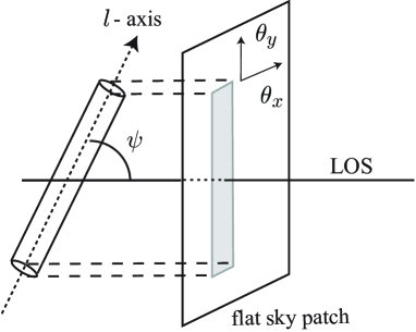
Figure 7: The projected filament on the flat sky patch ($\theta_{x},\theta_{y}$) is represented in gray. The observer is at the right end on the LOS. The filament has an inclination angle $\psi$ between the symmetrical axis (the $l$–axis) and the LOS.

We perform the Fourier transform of Eq. (23) in the 2-D flat space and we obtain the Fourier component,

$$\delta\tilde{T}_{b}(\ell_{x},\ell_{y})={2\pi\delta T_{b0}\over\ell_{x}\ell_{y}\sin\psi}{J_{1}\left({\ell_{x}r_{\rm t}\over 2D_{A}}\right)}\sin\left({\ell_{y}l_{l}\sin\psi\over 2D_{A}}\right).$$ (24)

Accordingly, the 2-D spectrum is simply given by

$$P_{2}(\ell_{x},\ell_{y})=\left[{2\pi\delta T_{b0}\over\ell_{x}\ell_{y}\sin\psi}{J_{1}\left({\ell_{x}r_{t}\over 2D_{A}}\right)}\sin\left({\ell_{y}l_{l}\sin\psi\over 2D_{A}}\right)\right]^{2}.$$ (25)

In order to get the power spectrum $P(\ell,L,\psi)$ at a given $\ell$, we must take into account the contributions from all $(\ell_{x},\ell_{y})$ which satisfy $\ell^{2}=\ell^{2}_{x}+\ell^{2}_{y}$,

$$P(\ell,L,\psi)={1\over\ell}\sum_{(\ell_{x},\ell_{y})}P_{2}(\ell_{x},\ell_{y}).$$ (26)

Using Eq. (21), we calculate the angular power spectrum for different $G\mu$. We represent the results of the angular power spectra in Fig. 8.

The amplitude of the spectrum depends on $G\mu$. Larger $G\mu$ produces higher amplitude of the angular power spectrum. The angular power spectrum due to loops does not have a strong redshift dependence. At small $\ell$, the spectrum $\ell^{2}C_{\ell}$ is proportional to $\ell$. However, the slope becomes shallow with increasing $\ell$, and the spectrum is almost constant at large $\ell$. The multipole at which the slope changes corresponds to the typical length scale of the filaments. For larger $G\mu$, since even small filaments can contribute to the spectrum, the multipole at which the slope changes shifts to larger $\ell$.

We found that most contributions come from filaments produced by small strings generated $z>z_{\rm eq}$. The length of such filaments is smaller than the width of the response function, $\Delta z=1$. Hence, as mentioned above, Eq. (23) is valid in our calculation.

The promising signal of the cosmological 21 cm fluctuations is provided by the primordial density fluctuations. For reference, we plot the angular power spectrum due to the primordial density fluctuations obtained through CAMB for the sharp window function Lewis:2007kz . At $z>30$, the angular power spectrum for $G\mu>10^{-8}$ can dominate the primordial fluctuations. Although the angular power spectrum induced by loops is almost independent of the redshift, the amplitude due to the primordial fluctuations becomes small as the redshift decreases. As a result, the spectrum due to loops dominate the primordial density fluctuations at low multipoles $\ell<1000$ at $z=20$ even for $G\mu=10^{-10}$.

In the power spectrum for $G\mu>10^{-8}$, most of the contributions are emission signals. On the other hand, the absorption signals dominate for $G\mu=10^{-10}$. This is because small $G\mu$ cannot produce massive filaments in which the filament gas heats up to the virial temperature larger than the CMB temperature. For $G\mu=10^{-9}$, absorption and emission contributions are comparable. Since the filament virial temperature grows with time, the absorption contribution becomes large at low redshifts. The 21 cm signals due to the primordial density fluctuations before the epoch of reionization are absorption signals. Hence the separation between the emission and absorption signals in a 21 cm map can facilitate measurement of the power spectrum due to loops with up to $G\mu\sim 10^{-9}$.

In order to access the detectability, we also plot the instrumental noise power spectrum based on the SKA design in Fig. 8. The instrumental noise power spectrum including the beam effects is given by Knox:1995dq

$${N_{\ell}^{21}}={2\pi\over t_{\rm obs}\Delta\nu}\left({\lambda T_{\rm sys}\over f_{\rm cover}D}\right)^{2}\exp\left[{\frac{\ell(\ell+1)}{\ell_{b}^{2}}}\right],$$ (27)

where $T_{\rm sys}$ is the system temperature, $f_{\rm cover}$ is the a covering fraction of the effective collecting area to the total collecting area, $t_{\rm obs}$ is the observation time, $\Delta\nu$ is the frequency bandwidth, $D$ is the length of the baseline and $\ell_{b}$ is given by $\ell_{b}=4\sqrt{\ln 2}/\theta_{fw}$ with the resolution $\theta_{fw}\sim\lambda/D$. We set the system temperature to the sky temperature in the region of the minimum emission at high Galactic latitude; $T_{\rm sys}=180(\nu/180{\rm MHz})^{-2.6}\rm K$. We choose $\Delta\nu$ corresponding to the redshift width $\Delta z=1$ and set $t_{\rm obs}=1~{}$year. The current design of SKA is $f_{\rm cover}=0.02$ and $D=6~{}$km. However, we take $f_{\rm cover}=0.2$ in this paper.

The noise power spectrum strongly depends on the redshift. At high redshift ($z=30$), the noise power spectrum totally overdominates the spectrum due to loops. However, at low redshift ($z=20$), the noise power spectrum in low multipoles becomes smaller than the spectrum for $G\mu=10^{-8}$, and is comparable to the one for $G\mu=10^{-9}$. Therefore, we conclude that the power spectrum due to loops with $G\mu=10^{-8}$ can be detected via 21 cm observations with high signal to noise ratio at low redshifts.

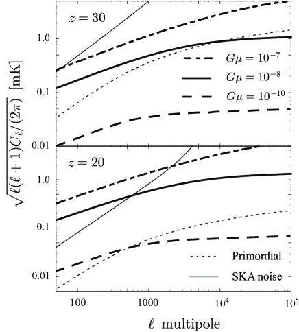
Figure 8: The angular power spectrum due to loops. In the left panel, we plot the spectra with $G\mu=10^{-7}$, $G\mu=10^{-8}$ and $G\mu=10^{-10}$ as the dot-dashed, solid and dashed lines, respectively. In the right panel, the solid line represents the total angular power spectrum for $G\mu=10^{-9}$, and the dashed and the dot-dashed lines show contributions from emission and absorption components, respectively. From top to bottom in both panels, we set $\nu_{\rm obs}$ corresponding to $z=30$, and $z=20$. For comparison, we show the spectrum due to the primordial density fluctuations with the dotted line. We also plot the noise power spectrum of the SKA-like observation as the gray line.

V conclusion

We have investigated the 21 cm signatures induced by cosmic string loops in this paper. We have taken into account that the loops have the initial relativistic velocities. A loop with an initial velocity can form a filament structure. We have evaluated the gas temperature inside a filament due to a loop and calculated the differential 21 cm brightness temperature profile. We have shown that a filament can induce an observable signal. The brightness temperature can reach $200$ mK for a loop with $G\mu\sim 10^{-7}$.

We have also calculated the angular power spectrum of 21 cm fluctuations due to loops with a scaling loop number density distribution. The larger $G\mu$ is, the higher the spectrum amplitude due to loops becomes. The power spectrum is proportional to $\ell$ on large scales, while it is scale-invariant on small scales. The scale where the slope of the spectrum changes corresponds to the typical length scale of the filaments. The spectrum does not strongly depend on the observation redshift.

We found that the amplitude of the spectrum due to the loops is larger than the one due to long strings evaluated in Ref. Hernandez:2011ym . Therefore, the angular power spectrum of 21 cm fluctuations can give the limit on $G\mu$ by measuring the spectrum due to loops. At $z=30$, the angular power spectrum for $G\mu>10^{-8}$ can dominate the spectrum of the primordial density fluctuations. The amplitude due to the primordial fluctuations becomes smaller as the redshift decreases. Hence, the amplitude of the spectrum even for $G\mu=10^{-10}$ can be larger than for the primordial density fluctuations at $z=20$. However, first galaxies formed around $z\sim 20$ produce the larger 21 cm fluctuations through the Ly-$\alpha$ flux and X-ray heating 2005ApJ…626….1B ; Pritchard:2006sq .

Comparing with the noise power spectrum of the 1 year SKA-like observation, we have found that the power spectrum for $G\mu=10^{-8}$ dominates the noise power spectrum at low multipoles ($\ell<1000$). Therefore, it is expected that the SKA-like observation can measure the spectrum for $G\mu>10^{-8}$ with high signal to noise ratio.

The amplitude of the spectrum depends on the loop number density distribution which is not completely understood. For example, the analytical work, Ref. Lorenz:2010sm , suggested scaling loop distribution with small loop production. Because of the difference in the distributions, we found that the angular power spectrum will be reduced by $\sim 0.1$ with the distribution in Ref. Lorenz:2010sm .

Since the filaments produced by loops are gravitationally unstable, they will fragment into beads, which subsequently merge into larger beads as considered in Ref. Shlaer:2012rj . Although we have not taken into account this effect in this paper, the fragmentation of the filaments decreases the amplitude of the spectrum on large scales and enhances on small scales. The evaluation of the power spectrum with the fragmentation effect requires a detailed study including numerical simulations. However, in order to evaluate the fragmentation effect roughly, we simply assume that the filaments collapse into beads with the filament width size which corresponds to the fastest growing instability mode and following mergers of beads makes the length of the beads ten times larger. Under this assumption, we found that the amplitude of the spectrum is decreased by 0.1 on large scales and enhanced roughly by 6 on small scales.

In our calculation of the angular power spectrum, we have only considered the contributions of small filaments whose virial temperature is below $10^{4}~{}$K. In massive filaments with the virial temperature larger than $10^{4}~{}$K, stars can be formed and ionize the surrounding IGM gas Shlaer:2012rj . The ionized gas can produce additional large 21 cm fluctuations. We will study the 21 cm power spectrum due to massive filaments in future work.

References

- (1) T. W. B. Kibble, J. Phys. A 9, 1387 (1976).
- (2) A. Vilenkin and E.P.S. Shellard. Cosmic Strings and Other Topological Defects (Cambridge University Press, Cambridge, England, 1994).
- (3) M. B. Hindmarsh and T. W. B. Kibble, Rept. Prog. Phys. 58, 477 (1995) [hep-ph/9411342].
- (4) N. Kaiser and A. Stebbins, Nature 310, 391 (1984).
- (5) U. Seljak, U. -L. Pen and N. Turok, Phys. Rev. Lett. 79, 1615 (1997) [astro-ph/9704231].
- (6) B. Allen, R. R. Caldwell, S. Dodelson, L. Knox, E. P. S. Shellard and A. Stebbins, Phys. Rev. Lett. 79, 2624 (1997) [astro-ph/9704160, astro-ph/9704160].
- (7) A. Albrecht, R. A. Battye and J. Robinson, Phys. Rev. Lett. 79, 4736 (1997) [astro-ph/9707129].
- (8) L. Pogosian, M. C. Wyman and I. Wasserman, JCAP 0409, 008 (2004) [astro-ph/0403268].
- (9) N. Bevis, M. Hindmarsh, M. Kunz and J. Urrestilla, Phys. Rev. D 76, 043005 (2007) [arXiv:0704.3800 [astro-ph]].
- (10) N. Bevis, M. Hindmarsh, M. Kunz and J. Urrestilla, Phys. Rev. Lett. 100, 021301 (2008) [astro-ph/0702223 [ASTRO-PH]].
- (11) L. Pogosian and M. Wyman, Phys. Rev. D 77, 083509 (2008) [arXiv:0711.0747 [astro-ph]].
- (12) A. A. Fraisse, C. Ringeval, D. N. Spergel and F. R. Bouchet, Phys. Rev. D 78, 043535 (2008) [arXiv:0708.1162 [astro-ph]].
- (13) M. Hindmarsh, C. Ringeval and T. Suyama, Phys. Rev. D 80, 083501 (2009) [arXiv:0908.0432 [astro-ph.CO]].
- (14) M. Hindmarsh, C. Ringeval and T. Suyama, Phys. Rev. D 81, 063505 (2010) [arXiv:0911.1241 [astro-ph.CO]].
- (15) D. M. Regan and E. P. S. Shellard, Phys. Rev. D 82, 063527 (2010) [arXiv:0911.2491 [astro-ph.CO]].
- (16) C. Dvorkin, M. Wyman and W. Hu, Phys. Rev. D 84, 123519 (2011) [arXiv:1109.4947 [astro-ph.CO]].
- (17) C. Ringeval and F. R. Bouchet, Phys. Rev. D 86, 023513 (2012) [arXiv:1204.5041 [astro-ph.CO]].
- (18) P. A. R. Ade et al. [Planck Collaboration], arXiv:1303.5085 [astro-ph.CO].
- (19) H. Tashiro, E. Sabancilar and T. Vachaspati, arXiv:1212.3283 [astro-ph.CO].
- (20) Y. -Z. Chu and T. Vachaspati, arXiv:1302.3222 [hep-th].
- (21) Y. .B. Zeldovich, Mon. Not. Roy. Astron. Soc. 192, 663 (1980).
- (22) A. Vilenkin, Phys. Rev. Lett. 46, 1169 (1981) [Erratum-ibid. 46, 1496 (1981)].
- (23) J. Silk and A. Vilenkin, Phys. Rev. Lett. 53, 1700 (1984).
- (24) M. J. Rees, Mon. Not. Roy. Astron. Soc. 222, 27 (1986).
- (25) T. Hara, S. Miyoshi and P. Maehoenen, Astrophys. J. 412, 22 (1993).
- (26) P. P. Avelino and A. R. Liddle, Mon. Not. Roy. Astron. Soc. 348, 105 (2004) [astro-ph/0305357].
- (27) L. Pogosian and A. Vilenkin, Phys. Rev. D 70, 063523 (2004) [astro-ph/0405606].
- (28) K. D. Olum and A. Vilenkin, Phys. Rev. D 74, 063516 (2006) [astro-ph/0605465].
- (29) B. Shlaer, A. Vilenkin and A. Loeb, JCAP 1205, 026 (2012) [arXiv:1202.1346 [astro-ph.CO]].
- (30) T. Vachaspati and A. Vilenkin, Phys. Rev. D 31, 3052 (1985).
- (31) T. Damour and A. Vilenkin, Phys. Rev. Lett. 85, 3761 (2000) [gr-qc/0004075].
- (32) T. Damour and A. Vilenkin, Phys. Rev. D 64, 064008 (2001) [gr-qc/0104026].
- (33) T. Damour and A. Vilenkin, Phys. Rev. D 71, 063510 (2005) [hep-th/0410222].
- (34) S. Olmez, V. Mandic and X. Siemens, Phys. Rev. D 81, 104028 (2010) [arXiv:1004.0890 [astro-ph.CO]].
- (35) R. van Haasteren, Y. Levin, G. H. Janssen, K. Lazaridis, M. K. B. W. Stappers, G. Desvignes, M. B. Purver and A. G. Lyne et al., arXiv:1103.0576 [astro-ph.CO].
- (36) S. A. Sanidas, R. A. Battye and B. W. Stappers, Phys. Rev. D 85, 122003 (2012) [arXiv:1201.2419 [astro-ph.CO]].
- (37) P. Binetruy, A. Bohe, C. Caprini and J. -F. Dufaux, JCAP 1206, 027 (2012) [arXiv:1201.0983 [gr-qc]].
- (38) S. Furlanetto, S. P. Oh and F. Briggs, Phys. Rept. 433, 181 (2006) [astro-ph/0608032].
- (39) J. R. Pritchard and A. Loeb, Rept. Prog. Phys. 75, 086901 (2012) [arXiv:1109.6012 [astro-ph.CO]].
- (40) P. Madau, A. Meiksin and M. J. Rees, Astrophys. J. 475, 429 (1997).
- (41) M. Tegmark and M. Zaldarriaga, Phys. Rev. D 82, 103501 (2010) [arXiv:0909.0001 [astro-ph.CO]].
- (42) R. Khatri and B. D. Wandelt, Phys. Rev. Lett. 100, 091302 (2008) [arXiv:0801.4406 [astro-ph]].
- (43) A. Berndsen, L. Pogosian and M. Wyman, Mon. Not. Roy. Astron. Soc. 407, 1116 (2010) [arXiv:1003.2214 [astro-ph.CO]].
- (44) R. H. Brandenberger, R. J. Danos, O. F. Hernandez and G. P. Holder, JCAP 1012, 028 (2010) [arXiv:1006.2514 [astro-ph.CO]].
- (45) O. F. Hernandez, Y. Wang, R. Brandenberger and J. Fong, JCAP 1108, 014 (2011) [arXiv:1104.3337 [astro-ph.CO]].
- (46) O. F. Hernandez and R. H. Brandenberger, JCAP 1207, 032 (2012) [arXiv:1203.2307 [astro-ph.CO]].
- (47) M. Pagano and R. Brandenberger, JCAP 1205, 014 (2012) [arXiv:1201.5695 [astro-ph.CO]].
- (48) T. Vachaspati and A. Vilenkin, Phys. Rev. D 30, 2036 (1984).
- (49) B. Allen and E. P. S. Shellard, Phys. Rev. Lett. 64, 119 (1990).
- (50) V. Vanchurin, K.D. Olum and A. Vilenkin, Phys. Rev. D 74, 063527 (2006) [arXiv:gr-qc/0511159].
- (51) C. Ringeval, M. Sakellariadou and F. Bouchet, JCAP 0702, 023 (2007) [arXiv:astro-ph/0511646].
- (52) K. D. Olum and V. Vanchurin, Phys. Rev. D 75, 063521 (2007) [arXiv:astro-ph/0610419].
- (53) G. Hinshaw et al. [WMAP Collaboration], arXiv:1212.5226 [astro-ph.CO].
- Bertschinger (1987) Bertschinger, E., Astrophys. J. 316, 489 (1987)
- (55) D. J. Eisenstein, A. Loeb and E. L. Turner, [astro-ph/9605126].
- (56) S. Dodelson, Amsterdam, Netherlands: Academic Pr. (2003) 440 p
- (57) M. Shimon, S. Sadeh and Y. Rephaeli, JCAP 1210, 038 (2012) [arXiv:1209.5065 [astro-ph.CO]].
- (58) B. Ciardi and P. Madau, Astrophys. J. 596, 1 (2003) [astro-ph/0303249].
- Field (1958) G. B. Field, Proceedings of the IRE 46, 240 (1985)
- Field (1959) G. B. Field, Astrophys. J. 129, 536 (1985)
- (61) M. Kuhlen, P. Madau and R. Montgomery, Astrophys. J. 637, L1 (2006) [astro-ph/0510814].
- (62) M. shimon, S. Sadeh and Y. Rephaeli, JCAP 1210, 038 (2012) [arXiv:1209.5065 [astro-ph.CO]].
- (63) S. Cole and N. Kaiser, MNRAS 233, 637 (1988).
- (64) S. Furlanetto and A. Loeb, Astrophys. J. 579, 1 (2002) [astro-ph/0206308].
- (65) J. J. Blanco-Pillado, K. D. Olum and B. Shlaer, Phys. Rev. D 83, 083514 (2011) [arXiv:1101.5173 [astro-ph.CO]].
- (66) L. Lorenz, C. Ringeval and M. Sakellariadou, JCAP 1010, 003 (2010) [arXiv:1006.0931 [astro-ph.CO]].
- (67) A. Lewis and A. Challinor, Phys. Rev. D 76, 083005 (2007) [astro-ph/0702600 [ASTRO-PH]].
- (68) L. Knox, Phys. Rev. D 52, 4307 (1995) [astro-ph/9504054].
- (69) R. Barkana and A. Loeb, Astrophys. J. 626, 1 (2005).
- (70) J. R. Pritchard and S. R. Furlanetto, Mon. Not. Roy. Astron. Soc. 376, 1680 (2007) [astro-ph/0607234].