Searching for New Physics through correlations of Flavour Observables

Abstract:

The coming flavour precision era will allow to uncover various patterns of flavour violation in different New Physics scenarios. We discuss different classes of them. A simple extension of the Standard Model that generally introduces new sources of flavour and CP violation as well as right-handed currents is the addition of a $U(1)$ gauge symmetry to the SM gauge group. In such $Z^{\prime}$ models correlations between various flavour observables emerge that could test and distinguish different $Z^{\prime}$ scenarios. A concrete model with flavour violating $Z^{\prime}$ couplings is the 331 model based on the gauge group $SU(3)_{C}\times SU(3)_{L}\times U(1)_{X}$. We also study tree-level FCNCs mediated by heavy neutral scalars and/or pseudo-scalars $H^{0}(A^{0})$. Furthermore the implications of an additional approximate global $U(2)^{3}$ flavour symmetry is shortly discussed. Finally a model with vectorlike fermions and flavour violating $Z$ couplings is presented. We identify a number of correlations between various observables that differ from those known from constrained minimal flavour violating (CMFV) models and that could test and distinguish these different scenarios.

1 Introduction

One highlight of LHCb so far was the measurement of $\overline{\mathcal{B}}(B_{s}\to\mu^{+}\mu^{-})^{\text{exp}}=(3.2^{+1.5}_{-1.2})\times 10^{-9}$ [1, 2]. This has to be compared to the SM prediction $\mathcal{B}(B_{s}\to\mu^{+}\mu^{-})^{\text{SM}}=(3.25\pm 0.17)\cdot 10^{-9}$ [3] and $\overline{\mathcal{B}}(B_{s}\to\mu^{+}\mu^{-})^{\text{SM}}=(3.56\pm 0.18)\cdot 10^{-9}$ [4] without and with including $\Delta\Gamma_{s}$ effects. So far everything is consistent with the SM and the room that is left for new physics (NP) gets smaller.

A slight tension in the flavour data concerns $|\varepsilon_{K}|$ and $S_{\psi K_{S}}$ which is related to the so-called $|V_{ub}|$-problem. Both $|\varepsilon_{K}|\propto\sin 2\beta|V_{cb}|^{4}$ and $S_{\psi K_{S}}$ can be used to determine $\sin 2\beta$. The value for $\sin 2\beta$ derived from the experimental value of $S_{\psi K_{S}}$ is much smaller that the one derived from $|\varepsilon_{K}|$ [5, 6]. The “true” value of the angle $\beta$ of the unitarity triangle depends on the value of $|V_{ub}|$ and $\gamma$. However there is a tension between the exclusive and inclusive determinations of $|V_{ub}|$ [7]:

$$|V_{ub}^{\text{incl.}}|=(4.27\pm 0.38)\cdot 10^{-3}\,,\qquad|V_{ub}^{\text{excl.}}|=(3.38\pm 0.36)\cdot 10^{-3}\,.$$ (1)

• Scenario 1 (S1): If one uses the exclusive value of $|V_{ub}|$ to derive $\beta_{\text{true}}$ and then calculates $S_{\psi K_{S}}^{\text{SM}}=\sin 2\beta_{\text{true}}$ one finds agreement with the data whereas $|\varepsilon_{K}|$ stays below the data.

• Scenario 2 (S2): Using the inclusive $|V_{ub}|$ as input for $\beta_{\text{true}}$, $S_{\psi K_{S}}$ is above the measurements while $|\varepsilon_{K}|$ is in agreement with the data.

However one has to keep in mind the error on $|\varepsilon_{K}|$ coming dominantly from the error of $|V_{cb}|$ and the error of the QCD factor $\eta_{1}$ [8]. Since $S_{\psi K_{S}}$ is a rather clean observable in the SM one would need a new CP violating phase in S2 to get agreement with the SM. When studying NP models it is interesting to see if this $|\varepsilon_{K}|-S_{\psi K_{S}}$ tension can be solved in this particular model and if yes, which scenario is chosen by the model. CMFV chooses for example S1 because there are no new phases whereas the 331 model which I will discuss below chooses S2 as effects in $\varepsilon_{K}$ are rather small and a new phase enters $B_{d}$-mixing.

2 Phenomenology of $Z^{\prime}$, new (pseudo) scalar $A^{0}/H^{0}$ and vectorlike fermions

What is the first new particle beyond the Higgs to be discovered at the LHC? Is it a new heavy gauge boson, a heavy (pseudo) scalar or a heavy vectorlike fermion? If it is too heavy for a direct discovery then we can only see it in high precision flavour experiments. In the following I will first discuss a concrete model where FCNC are induced by a $Z^{\prime}$ [10]. Afterwards this approach is extended to more general $Z^{\prime}$ and also scalar scenarios [11, 4]. At the end I present a model with vectorlike fermions [12]. A summary of the implications of LHCb measurements on further models like Little Higgs, Randall Sundrum, SUSY GUTs can be found in [13].

2.1 Concrete model with $Z^{\prime}$ FCNC: 331 model

The 331 model is based on the gauge group $SU(3)_{C}\times SU(3)_{L}\times U(1)_{X}$. In the breaking $SU(3)_{L}\times U(1)_{X}\to SU(2)_{L}\times U(1)_{Y}$ to the SM gauge group a new heavy neutral gauge boson $Z^{\prime}$ appears that mediates FCNC already at tree level. A nice theoretical feature is that we have an explanation of why there are $N=3$ generations. This follows from the requirement of anomaly cancellation and asymptotic freedom of QCD. Anomaly cancellation is only possible if one generation (usually the 3${}^{\text{rd}}$ is chosen) is treated differently than the other two generations.

Flavour structure

There are different versions of the 331 model characterized by a parameter $\beta$ that determines the particle content. We consider $\beta=1/\sqrt{3}$ (to be called $\overline{331}$ model) with the following fermion content: Left-handed fermions fit in (anti)triplets, while right-handed ones are singlets under $SU(3)_{L}$. In the quark sector, the first two generations fill the two upper components of a triplet, while the third one fills those of an anti-triplet; the third member of the quark (anti)triplet is a new heavy fermion:

$$\begin{pmatrix}e\\ -\nu_{e}\\ \nu_{e}^{c}\end{pmatrix}_{L}\,,\begin{pmatrix}\mu\\ -\nu_{\mu}\\ \nu_{\mu}^{c}\end{pmatrix}_{L}\,,\begin{pmatrix}\tau\\ -\nu_{\tau}\\ \nu_{\tau}^{c}\end{pmatrix}_{L}\,,\quad\qquad\begin{pmatrix}u\\ d\\ D\end{pmatrix}_{L}\,,\begin{pmatrix}c\\ s\\ S\end{pmatrix}\,,\begin{pmatrix}b\\ -t\\ T\end{pmatrix}_{L}$$ (2)

$$e_{R},\,\mu_{R},\,\tau_{R},\,\qquad u_{R},\,d_{R},\,c_{R},\,s_{R},\,t_{R},\,b_{R},\,\qquad D_{R},S_{R},T_{R}$$ (3)

Due to anomaly cancellation we need the same number of triplets and anti-triplets. If one takes into account the three colours of the quarks we have six triplets and six anti-triplets with this choice. Neutral currents mediated by $Z^{\prime}$ are affected by the quark mixing since the $Z^{\prime}$ couplings are generation non-universal. In order to see this explicitly, we look at $Z^{\prime}$ couplings to SM quarks:

$$\mathcal{L}^{Z^{\prime}}=J_{\mu}Z^{\prime\mu}\,,\quad\quad V_{\text{CKM}}=U_{L}^{\dagger}V_{L},$$ (4)

$$J_{\mu}=\bar{u}_{L}\gamma_{\mu}U_{L}^{\dagger}\begin{pmatrix}a&&\\ &a&\\ &&b\end{pmatrix}U_{L}u_{L}+\bar{d}_{L}\gamma_{\mu}V_{L}^{\dagger}\begin{pmatrix}a&&\\ &a&\\ &&b\end{pmatrix}V_{L}d_{L}\,.$$ (5)

The unitary rotation matrices $U_{L},V_{L}$ do not cancel out for $a\neq b$ but generate tree-level FCNCs $\propto(b-a)$. However only left-handed (LH) quark currents are flavour-violating. In Sec. 2.2 we will generalize this and include also right-handed (RH) currents. We choose a parametrization for $V_{L}$ using 3 angles and 3 phases $\tilde{s}_{12},\tilde{s}_{23},\tilde{s}_{13},\delta_{1,2,3}$ such that the $B_{d}$ sector depends only on $\tilde{s}_{13},\delta_{1}$, the $B_{s}$ sector on $\tilde{s}_{23},\delta_{2}$ but then the $K$ sector is correlated and depends on the same angles $\tilde{s}_{13},\tilde{s}_{23}$ and the phase difference $\delta_{2}-\delta_{1}$. In more general models in Sec. 2.2 the $K$ sector is then decoupled from $B_{d,s}$ sector.

Finding optimal oases in parameter space

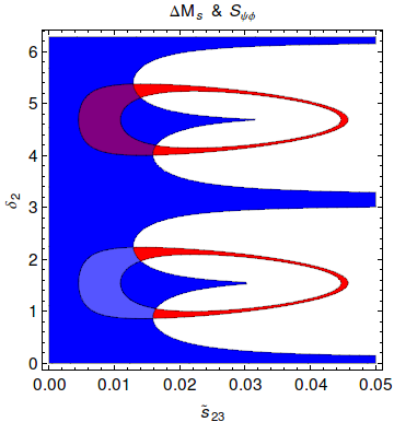
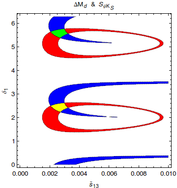
Figure 1: Ranges for $\Delta M_{s,d}$ (red) and $S_{\psi\phi}/S_{\psi K_{S}}$ (blue) satisfying the bounds in Eq. (6) and (7). The plot on the left is obtained for $M_{Z^{\prime}}=1$ TeV and $|V_{ub}|=0.004$. The purple, blue, green and yellow regions define our oases.

Our strategy that we will also adopt in the more general scenarios in Sec. 2.2 is the following: we look first at $\Delta F=2$ observables to find constraints on the free parameters $\tilde{s}_{ij}$ and $\delta_{i}$. In order to find these “oases” in the parameter space we require that the mixing induced CP asymmetries are within their experimental 2$\sigma$ range and for the mass differences $\Delta M_{d,s}$ we take only 5% error assuming a flavour precision era ahead of us:

$$16.9~{}{\rm ps}^{-1}\leq\Delta M_{s}\leq 18.7~{}{\rm ps}^{-1},\quad-0.18\leq S_{\psi\phi}\leq 0.18,$$ (6)

$$0.48~{}{\rm ps}^{-1}\leq\Delta M_{d}\leq 0.53~{}{\rm ps}^{-1},\quad 0.64\leq S_{\psi K_{S}}\leq 0.72.$$ (7)

Within these oases we then also include $\Delta F=1$ observables in order to find correlations between different observables. Such correlations can help to identify and distinguish between different NP models. In Fig. 1 we show the two oases for $B_{s}$ and $B_{d}$ system, respectively. We use $M_{Z^{\prime}}=1~{}$TeV and $|V_{ub}|=0.004$ such that $S_{\psi K_{S}}$ must be suppressed below its SM value. Due to the appearance of the phase $\delta_{1}$ this is indeed possible. The two-fold ambiguity between $\delta_{1,2}$ and $\delta_{1,2}+\pi$ can be resolved with $\Delta F=1$ observables (see Fig. 2). Here $S_{\mu^{+}\mu^{-}}^{s}$ corresponds to a tagged time-dependent CP asymmetry of $B_{s}\to\mu^{+}\mu^{-}$ [14]. Fig. 2 shows that we have a triple correlation $S_{\mu^{+}\mu^{-}}^{s}-S_{\psi\phi}-\mathcal{B}(B_{s}\to\mu^{+}\mu^{-})$: once the sign of $S_{\mu^{+}\mu^{-}}^{s}$ is known a unique correlation $S_{\psi\phi}-\mathcal{B}(B_{s}\to\mu^{+}\mu^{-})$ is found. If in addition one of these three observables is precisely known the other two can be strongly constrained. Effects in $B_{d}\to\mu^{+}\mu^{-}$ are rather small but one can see that in one oasis we find enhancement and in the other a slight suppression w.r.t. SM central value. The new contributions in $K$ sector, especially in $\varepsilon_{K}$, $K_{L}\to\pi^{0}\bar{\nu}\nu$ and $K^{+}\to\pi^{+}\bar{\nu}\nu$ turned out to be negligible. However the $S_{\psi K_{S}}-\varepsilon_{K}$ tension explained in Sec. 1 could be solved using $|V_{ub}|=0.004$.

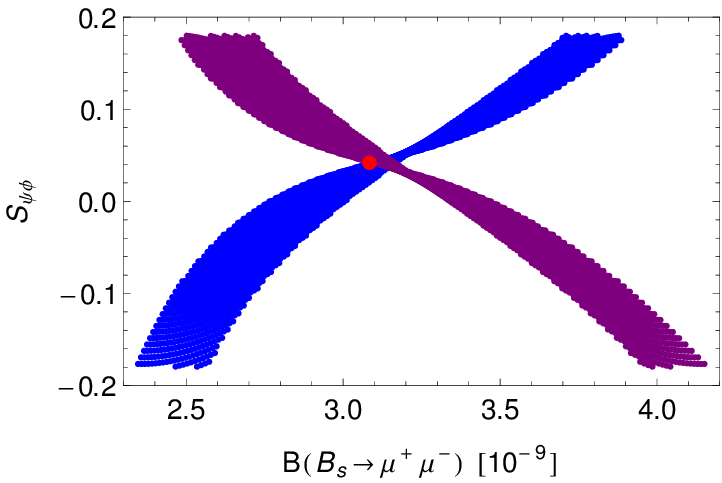
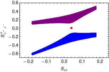
Figure 2: $S_{\psi\phi}$ vs. $B_{s}\to\mu^{+}\mu^{-}$, $S_{\mu^{+}\mu^{-}}^{s}$ vs. $S_{\psi\phi}$ and $S_{\psi K_{S}}$ vs. $B_{d}\to\mu^{+}\mu^{-}$ within the oases from Fig. 1

2.2 General $Z^{\prime}$ and $A^{0}/H^{0}$ scenarios

The approach of the previous section is now generalized including both left-and right-handed $Z^{\prime}$/(pseudo)scalar FCNC couplings (see Fig. 3). We distinguish between different scenarios: LHS (RHS): $\Delta_{L(R)}\neq 0=\Delta_{R(L)}$, LRS: $\Delta_{L}=\Delta_{R}$ and ALRS $\Delta_{L}=-\Delta_{R}$. In addition we now also have to make assumptions about the lepton couplings. In the 331 model this came out automatically from the Lagrangian: $\Delta_{L}^{\nu\bar{\nu}}(Z^{\prime})=0.14$ and $\Delta_{A}^{\mu\bar{\mu}}(Z^{\prime})=-0.26$. For the general $Z^{\prime}$ scenario we set the lepton couplings at $\Delta_{L}^{\nu\bar{\nu}}(Z^{\prime})=0.5$ and $\Delta_{A}^{\mu\bar{\mu}}(Z^{\prime})=0.5$. In the SM both couplings of $Z$ are equal to $0.372$. In the scalar scenario we set $\Delta_{P}^{\mu\bar{\mu}}(H)=0.020$ and $\Delta_{S}^{\mu\bar{\mu}}(H)=0.040$ (for more details see [11]).

Moreover we analyze what happens if an additional $U(2)^{3}$ global flavour symmetry is imposed. In this case the $K$ system is governed by MFV but $B_{d}$ and $B_{s}$ systems are now correlated [15]. Consequently instead of two separate oases plots for $B_{d}$ and $B_{s}$ system we now have only one for all four observables. As pointed out in [16, 17] a triple correlation $S_{\psi K_{S}}-S_{\psi\phi}-|V_{ub}|$ occurs such that now the $B_{s}$ oases depend also on $|V_{ub}|$.

Figure 3: Feynman rules for$Z^{\prime}$ and neutral scalar particle $H^{0}$ ($i,\,j$ denote different quark flavours and $\alpha,\,\beta$ the colours).

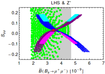
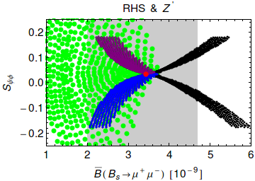
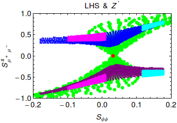
Figure 4: $S_{\psi\phi}$ vs. $B_{s}\to\mu^{+}\mu^{-}$ in LHS (top left) and RHS (top right), $S_{\mu^{+}\mu^{-}}^{s}$ vs. $S_{\psi\phi}$ in LHS (down left) and $B\to K\nu\bar{\nu}$ vs $B_{s}\to\mu^{+}\mu^{-}$ for both LHS and RHS (down right) for $M_{Z^{\prime}}=1~{}$TeV. The green points indicate the regions that are compatible with $b\to s\ell^{+}\ell^{-}$ constraints of [18]. Black points in RHS show the excluded area due to $b\to s\ell^{+}\ell^{-}$ transitions explicitly. Magenta and cyan regions correspond to the $U(2)^{3}$ limit for small and large $|V_{ub}|$.

In Fig. 4 the correlation $S_{\psi\phi}$ vs. $B_{s}\to\mu^{+}\mu^{-}$ for general $Z^{\prime}$ scenario is presented. The difference between LHS and RHS is that the two oases are interchanged. Furthermore the black points in RHS show explicitly the regions that are excluded due to $b\to s\ell^{+}\ell^{-}$ transitions where we used constraints derived in [18]. The green points indicate the regions that are compatible with $b\to s\ell^{+}\ell^{-}$ transitions. As one can see these constraints restrict the RHS more than the LHS. The magenta and cyan regions corresponds to the $U(2)^{3}$ limit for $|V_{ub}|=0.0031$ and $0.004$, respectively. For small $|V_{ub}|$ it follows that $S_{\psi\phi}$ is mainly negative. We also show $S_{\mu^{+}\mu^{-}}^{s}$ vs. $S_{\psi\phi}$ which is very similar to the middle plot in Fig. 2 of the 331 model, because it’s both for left-handed flavour changing $Z^{\prime}$ currents. A possibility to distinguish between LHS and RHS is through $b\to s\bar{\nu}\nu$ transitions (see down right in Fig. 4) where the brown/black points correspond to RHS and the blue ones to LHS.

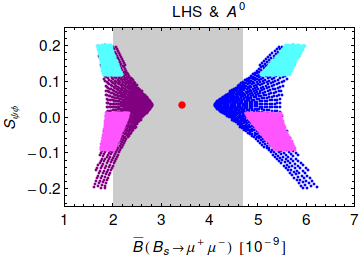
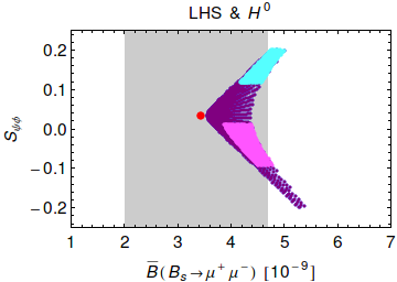
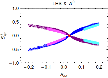
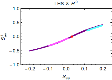
Figure 5: $S_{\psi\phi}$ vs. $B_{s}\to\mu^{+}\mu^{-}$ in LHS (top) and $S_{\mu^{+}\mu^{-}}^{s}$ vs. $S_{\psi\phi}$ (down) for pseudoscalar $A^{0}$ (left) and scalar $H^{0}$ (right) in LHS for $M_{H}=1~{}$TeV.

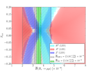
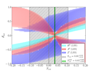
Figure 6: Overlay of the correlations for $S_{\psi\phi}$ vs. $B_{s}\to\mu^{+}\mu^{-}$ and $S_{\mu\mu}^{s}$ vs. $S_{\psi\phi}$ for tree level scalar (cyan), pseudoscalar (red) and $Z^{\prime}$ (blue) exchange (both oases in same colour respectively) in LHS. The lepton couplings are varied in the ranges $|\Delta_{S,P}^{\mu\mu}(H)|\in[0.02,0.04]$ and $\Delta_{A}^{\mu\mu}(Z^{\prime})\in[0.3,0.7]$.

Correlations in the $B_{s}$ system for pseudoscalar and scalar scenario are shown in Fig. 5 where also the $U(2)^{3}$ limit is included. In the scalar case the two oases cannot be distinguished and in $B_{s}\to\mu^{+}\mu^{-}$ only enhancement is possible. In the pseudoscalar case both constructive and destructive interference with the SM contribution is possible and effects can in principle be larger. The constraints from $b\to s\ell^{+}\ell^{-}$ transitions do not have any impact in the (pseudo) scalar case as shown in Ref. [11]. These results can now be compared with the corresponding plots for $Z^{\prime}$ case in Fig. 4. We observe striking differences between the results for $Z^{\prime}$, $A^{0}$ and $H^{0}$ scenario due to their different spin and CP quantum numbers. A summary plot is shown in Fig. 6 where now also the lepton couplings are varied in a wider range.

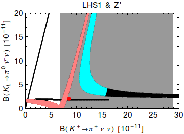
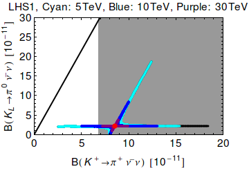
Figure 7: $K_{L}\to\pi^{0}\nu\bar{\nu}$ vs. $K^{+}\to\pi^{+}\nu\bar{\nu}$ in LHS1 for $M_{Z^{\prime}}=1~{}$TeV (left), 5/10/30 TeV (right). Black regions are excluded by the upper bound $\mathcal{B}(K_{L}\to\mu^{+}\mu^{-})\leq 2.5\cdot 10^{-9}$. Red point: SM central value. Gray region: experimental range of $\mathcal{B}(K^{+}\to\pi^{+}\nu\bar{\nu})$.

Results for Kaon sector in $Z^{\prime}$ scenario are shown in Fig. 7. Since only vector currents occur here there is no difference between LHS and RHS. The deviations from the SM are significantly larger than in the case of rare $B$ decays. This is a consequence of the weaker constraint from $\Delta S=2$ processes compared to $\Delta B=2$ and the fact that rare $K$ decays are stronger suppressed than rare $B$ decays within the SM. In $H^{0}/A^{0}$ scenario we expect negligible effects in channels with neutrinos.

2.3 New vectorlike fermions: a minimal theory of fermion masses

We now turn to a model with vectorlike fermions based on [19, 12] that can be seen as a Minimal Theory of Fermion Masses (MTFM). The idea is to explain SM fermion masses and mixings by their dynamical mixing with new heavy vectorlike fermion $F$. Very simplified the Lagrangian has the following form: $\mathcal{L}\propto m\bar{f}F+M\bar{F}F+\lambda hFF$, where $M$ denotes the heavy mass scale, $m$ characterizes the mixing and $\lambda$ is a Yukawa coupling. Thus the light fermions have an admixture of heavy fermions with explicit mass terms. The Higgs couples only to vectorlike but not to chiral fermions, so that SM Yukawas arise solely through mixing. We reduce the number of parameters such that it is still possible to reproduce the SM Yukawa couplings and that at the same time flavour violation is suppressed. In this way we can identify the minimal FCNC effects. A central formula is the leading order expression for the SM quark masses

$$m_{ij}^{X}=v\varepsilon_{i}^{Q}\varepsilon_{j}^{X}\lambda_{ij}^{X}\,,\qquad(X=U,D)\,,\qquad\varepsilon_{i}^{Q,U,D}=\frac{m_{i}^{Q,U,D}}{M_{i}^{Q,U,D}}\,.$$ (8)

In [19] the heavy Yukawa couplings $\lambda^{U,D}$ have been assumed to be anarchical $\mathcal{O}(1)$ real numbers which allowed a first look at the phenomenological implications. In [12] the so called TUM (Trivially Unitary Model) was studied in more detail. We assumed universality of heavy masses $M_{i}^{Q}=M_{i}^{U}=M_{i}^{D}=M$ and unitary Yukawa matrices. With this the flavour structure simplified considerably. Furthermore we concentrated on flavour violation in the down sector and thus set $\lambda^{U}=\mathds{1}$. After fitting the SM quark masses and the CKM matrix we are left with only four new real parameters and no new phases: $M,\,\varepsilon_{3}^{Q},\,s_{13}^{d},\,s_{23}^{d}$. The latter two parameters are angles of $\lambda^{D}$ (the third angle is fixed by the fitting procedure) and from fitting $m_{t}$ it follows that $0.8\leq\varepsilon_{3}^{Q}\leq 1$.

The new contributions to FCNC processes are dominated by tree-level flavour violating $Z$ couplings to quarks. The simplest version of the MTFM, the TUM, is capable of describing the known quark mass spectrum and the elements of the CKM matrix favoring $|V_{ub}|\approx 0.0037$. Since there are no new phases $S_{\psi K_{S}}$ stays SM-like and thus the large inclusive value of $|V_{ub}|$ is disfavored. Although effects in $\varepsilon_{K}$ can in principle be large, the effects are bounded by

$$\mathcal{B}(K_{L}\to\mu^{+}\mu^{-})_{\rm SD}\leq 2.5\cdot 10^{-9}\,.$$ (9)

For a $|V_{ub}|$ in between excl. and incl. value it is still possible to find regions in the parameter space that satisfy

$$0.75\leq\frac{\Delta M_{K}}{(\Delta M_{K})_{\rm SM}}\leq 1.25,\qquad 2.0\times 10^{-3}\leq|\varepsilon_{K}|\leq 2.5\times 10^{-3}$$ (10)

and Eq. (9) but then the prediction of the model is that $S_{\psi K_{S}}\approx 0.72$ which is by $2\sigma$ higher than its present experimental central value. In Fig. 8 (left) we show the correlation $\mathcal{B}(K_{L}\to\mu^{+}\mu^{-})$ vs. $|\varepsilon_{K}|$ for $M=3~{}$TeV where only the green points satisfy (9) and (10) simultaneously. In the TUM effects in $B_{s,d}$ mixings are negligible and the pattern of deviations from SM predictions in rare $B$ decays is CMFV-like as can be see on the right hand side of Fig. 8. However $\mathcal{B}(B_{s,d}\to\mu^{+}\mu^{-})$ are uniquely enhanced over their SM values. For $M=3~{}$TeV these enhancements amount to at least $35\%$ and can be as large as a factor of two. With increasing $M$ the enhancements decrease. However they remain sufficiently large for $M\leq 5~{}$TeV to be detected in the flavour precision era. Also effects in $K\to\pi\nu\bar{\nu}$ transitions are enhanced by a similar amount.

Figure 8: $\mathcal{B}(K_{L}\to\mu^{+}\mu^{-})$ vs. $|\varepsilon_{K}|$ and $\mathcal{B}(B_{d}\to\mu^{+}\mu^{-})$ vs. $\overline{\mathcal{B}}(B_{s}\to\mu^{+}\mu^{-})$ for $M=3~{}$TeV and $|V_{ub}|=0.0037$. Green points are compatible with both bounds for $|\varepsilon_{K}|$ (10) and $\mathcal{B}(K_{L}\to\mu^{+}\mu^{-})$ (9), yellow is only compatible with $|\varepsilon_{K}|$ and purple only with $\mathcal{B}(K_{L}\to\mu^{+}\mu^{-})$. The red point corresponds to the SM central value.

3 Summary

Correlations of flavour observables can help in identifying NP. We concentrated on rather simple extensions of the SM, namely those with tree-level FCNCs mediated by a $Z^{\prime}$, by an additional (pseudo) scalar $A^{0}/H^{0}$ or by the SM $Z^{0}$. The latter appeared in a model with new vectorlike fermions, the so-called TUM where $B_{d,s}\to\mu^{+}\mu^{-}$ are CMFV-like but enhanced. The $\overline{331}$ model is a concrete model with $Z^{\prime}$ FCNCs that are purely left-handed. Correlations of observables like $S_{\psi\phi}$, $B_{s}\to\mu^{+}\mu^{-}$ and $S_{\mu\mu}^{s}$ differ between $A^{0}$, $H^{0}$ and $Z^{\prime}$ case due to different spin and CP-parity which allow to distinguish between these scenarios. Rare Kaon decays $K\to\pi\nu\bar{\nu}$ play an important role even if the $Z^{\prime}$ mass is outside the reach of the LHC. One consequence of imposing an additional $U(2)^{3}$ flavour symmetry is that observables in the $B_{s}$ sector, especially the correlation between $S_{\psi\phi}$ and $B_{s}\to\mu^{+}\mu^{-}$ depends on $|V_{ub}|$ [16]. With improved experimental data and improved lattice calculations these correlation will allow to monitor how the simple NP scenarios face the future precision flavour data.

- [1] R. Aaij et al. [LHCb Collaboration], Phys. Rev. Lett. 108 (2012) 231801 [arXiv:1203.4493 [hep-ex]].
- [2] RAaij et al. [LHCb Collaboration], Phys. Rev. Lett. 110 (2013) 021801 [arXiv:1211.2674 [hep-ex]]
- [3] A. J. Buras, J. Girrbach, D. Guadagnoli and G. Isidori, Eur. Phys. J. C 72 (2012) 2172 [arXiv:1208.0934 [hep-ph]].
- [4] A. J. Buras, R. Fleischer, J. Girrbach and R. Knegjens, arXiv:1303.3820 [hep-ph].
- [5] E. Lunghi and A. Soni, Phys. Lett. B 666 (2008) 162 [arXiv:0803.4340 [hep-ph]].
- [6] A. J. Buras and D. Guadagnoli, Phys. Rev. D 78 (2008) 033005 [arXiv:0805.3887 [hep-ph]].
- [7] K. Nakamura et al. [Particle Data Group Collaboration], J. Phys. G 37 (2010) 075021.
- [8] J. Brod and M. Gorbahn, Phys. Rev. Lett. 108 (2012) 121801 [arXiv:1108.2036 [hep-ph]].
- [9] A. J. Buras and J. Girrbach, arXiv:1304.6835 [hep-ph].
- [10] A. J. Buras, F. De Fazio, J. Girrbach and M. V. Carlucci, JHEP 1302 (2013) 023 [arXiv:1211.1237 [hep-ph]].
- [11] A. J. Buras, F. De Fazio, J. Girrbach, R. Knegjens and M. Nagai, arXiv:1303.3723 [hep-ph].
- [12] A. J. Buras, J. Girrbach and R. Ziegler, JHEP 1304 (2013) 168 [arXiv:1301.5498 [hep-ph]].
- [13] A. J. Buras and J. Girrbach, Acta Phys. Polon. B 43 (2012) 1427 [arXiv:1204.5064 [hep-ph]].
- [14] K. De Bruyn, R. Fleischer, R. Knegjens, P. Koppenburg, M. Merk, A. Pellegrino and N. Tuning, Phys. Rev. Lett. 109 (2012) 041801 [arXiv:1204.1737 [hep-ph]].
- [15] R. Barbieri, G. Isidori, J. Jones-Perez, P. Lodone and D. M. Straub, Eur. Phys. J. C 71 (2011) 1725 [arXiv:1105.2296 [hep-ph]].
- [16] A. J. Buras and J. Girrbach, JHEP 1301 (2013) 007 [arXiv:1206.3878 [hep-ph]].
- [17] J. Girrbach, arXiv:1208.5630 [hep-ph].
- [18] W. Altmannshofer and D. M. Straub, JHEP 1208 (2012) 121 [arXiv:1206.0273 [hep-ph]].
- [19] A. J. Buras, C. Grojean, S. Pokorski and R. Ziegler, JHEP 1108 (2011) 028 [arXiv:1105.3725 [hep-ph]].