The Host Halos of OI Absorbers in the Reionization Epoch

Abstract

We use a radiation hydrodynamic simulation of the hydrogen reionization epoch to study OI absorbers at $z\sim 6$. The intergalactic medium (IGM) is reionized before it is enriched, hence OI absorption originates within dark matter halos. The predicted abundance of OI absorbers is in reasonable agreement with observations. At $z=10$, $\approx 70\%$ of sightlines through atomically-cooled halos encounter a visible ($N_{\mathrm{OI}}>10^{14}$cm^-2) column. Reionization ionizes and removes gas from halos less massive than $10^{8.4}M_{\odot}$, but 20% of sightlines through more massive halos encounter visible columns even at $z=5$. The mass scale of absorber host halos is 10–100$\times$ smaller than the halos of Lyman break galaxies and Lyman-$\alpha$ emitters, hence absorption probes the dominant ionizing sources more directly. OI absorbers have neutral hydrogen columns of $10^{19}$–$10^{21}$cm^-2, suggesting a close resemblance between objects selected in OI and HI absorption. Finally, the absorption in the foreground of the $z=7.085$ quasar ULASJ1120+0641 cannot originate in a dark matter halo because halo gas at the observed HI column density is enriched enough to violate the upper limits on the OI column. By contrast, gas at less than one third the cosmic mean density satisfies the constraints. Hence the foreground absorption likely originates in the IGM.

1 Introduction

Mapping out the progress of hydrogen reionization and understanding the nature of the sources that drove it constitute two of the central challenges that Astronomy will confront over the coming decade (National Academies Press, 2010). The cosmic microwave background constrains reionization to be roughly 50% complete at some point between $z=$9–11.8, although the results depend on the shape of the assumed reionization history (Hinshaw et al., 2012; Mitra et al., 2012; Pandolfi et al., 2011). The classic approach of measuring the neutral hydrogen fraction directly from the Lyman-$\alpha$ forest becomes increasingly difficult at redshifts beyond $z=6$ owing to the fact that Lyman-$\alpha$ absorption saturates for neutral hydrogen fractions in excess of $10^{-3}$ (Fan et al., 2002). In response to this challenge, a number of alternative techniques have been developed involving the abundance of Lyman-$\alpha$ emitters (Ouchi et al., 2010; Treu et al., 2012) or Lyman break galaxies (Muñoz & Loeb, 2011; Finkelstein et al., 2012; Robertson et al., 2013; Oesch et al., 2013), the statistics of dark pixels or gaps in the Lyman-$\alpha$ forest (Mesinger, 2010; McGreer et al., 2011), or the presence of damping wings in quasar spectra (Bolton et al., 2011; Schroeder et al., 2013). Each of these approaches combines unique strengths and weaknesses, hence it is necessary to consider a diverse variety of approaches together in order to overcome the weaknesses of any individual one.

One probe that has received relatively little attention involves the study of low-ionization metal absorbers (Oh, 2002; Furlanetto & Loeb, 2003). If diffuse regions of the pre-reionization intergalactic medium (IGM) were enriched with metals whose ionization potential is similar to that of hydrogen, then it may be possible to measure the ionization state of the metals directly and use this to trace the ionization state of the IGM as a whole. Recently, Becker et al. (2011) searched for low-ionization metal absorbers in moderate- and high-resolution spectra of 17 quasars at redshifts 5.8–6.4. They found that the abundance of systems at $z\sim 6$ roughly matches the combined number density of damped Ly$\alpha$ systems (DLAs; $2\times 10^{20}<N_{\mathrm{HI}}/\mathrm{cm}^{-2}$) and sub-DLAs ($10^{19}<N_{\mathrm{HI}}/\mathrm{cm}^{-2}<2\times 10^{20}$) at $z\sim 3$. Furthermore, the velocity widths of the high-redshift absorbers are similar to those of the DLAs, although with weaker equivalent widths. The authors concluded that low-ionization metal absorbers trace low-mass halos rather than neutral regions in the diffuse IGM.

Modeling OI absorbers in order to study the viability of this scenario requires a model that treats the inhomogeneous ionization and metal enrichment fields simultaneously. In Oppenheimer et al. (2009), we used a cosmological hydrodynamic simulation that assumed a spatially-homogeneous extragalactic ultraviolet ionizing background (EUVB) to study metal absorbers in the reionization epoch. The ionization field was adjusted in post-processing to consider scenarios in which there was no EUVB, a spatially-homogeneous EUVB, and an inhomogeneous model in which the EUVB at any point was dominated by the nearest galaxy. It was found that the OI absorber abundance was dramatically overproduced in the absence of an EUVB, and underproduced under the assumption of an optically-thin EUVB or a simple model in which the EUVB at any point was governed by the nearest galaxy. This work neglected two important aspects of the radiation field: First, the clustered nature of ionizing sources means that the EUVB at any point is determined by the combined influence of many galaxies rather than just the nearest one (Barkana & Loeb, 2004; Furlanetto et al., 2004a, b; Furlanetto & Oh, 2005). Second, dense sources acquire a multiphase ionization structure consisting of an optically-thick core and an optically-thin atmosphere. Modeling the ionization front that separates these phases requires a spatial resolution of $~{}\sim 1$ physical kpc (Schaye, 2001; Gnedin & Fan, 2006; McQuinn et al., 2011), which was not achievable through the simple treatment adopted in Oppenheimer et al. (2009). For these reasons, the spatial dependence of the assumed radiation field was incorrect. Hence while our previous study confirmed that there is enough oxygen to account for observations, the crude treatment of the EUVB meant that direct comparison with observations was preliminary.

Here, we remedy these deficiencies by studying the nature of OI absorption using cosmological simulations in which the EUVB and the galaxies are modeled simultaneously and self-consistently. We focus on OI absorbers because the abundance of oxygen leads to high OI columns while the proximity of its ionization potential to that of hydrogen means that the neutral oxygen fraction can be obtained trivially from the neutral hydrogen fraction. The goals of the current study are: (1) To study the relative spatial distributions of enriched and ionized gas and determine which portion of the IGM OI observations likely probe; (2) To understand the impact of reionization on the sources of OI absorption; (3) To compare the predicted and observed abundances of OI absorbers; and (4) to compare the HI and OI absorption properties of halo gas in the reionization epoch. Additionally, we will use our model to interpret observational constraints on the abundance of OI in the absorbing system that lies in the foreground of the $z=7.085$ quasar ULASJ1120+0641 (Mortlock et al., 2011).

In Section 2, we introduce our simulations. In Section 3, we explore the spatially-inhomogeneous ionization and chemical enrichment fields in our simulations. In Section 4, we use insights from our simulations to model the abundance of neutral oxygen absorbers as a function of redshift and compare with observations. We also compare the predicted HI and OI absorption properties of reionization-epoch halos. In Section 5 we discuss our results with an eye toward future modeling efforts, and in Section 6 we summarize.

2 Simulating Reionization and Enriched Outflows

2.1 Simulations

We use hydrodynamic simulations to model the inhomogeneous ionization and metallicity fields. These simulations are built on the parallel N-body + smoothed particle hydrodynamics (SPH) code Gadget-2 (Springel, 2005) and include treatments for radiative cooling, star formation, and momentum-driven galactic outflows (except for one simulation as we describe below). We model the EUVB on-the-fly by solving the moments of the radiation transport equation on a Cartesian grid that is superposed on our simulation volume. The ionizing emissivity within each cell is determined by the local star formation rate density, with a metallicity weighting based on the stellar population models of Schaerer (2003). The fraction of ionizing photons that escape into the IGM varies depending on the simulation (see below). The radiation and ionization fields are updated simultaneously using an iterative procedure. For details on all of these ingredients, see Finlator et al. (2011b, 2012).

Three of the four simulations account for the ability for dense gas to acquire an optically-thick core on spatial scales beneath the resolution limit of our radiation transport solver. We introduced this subgrid treatment in Finlator et al. (2012), but we review it here as it is a critical ingredient for modeling low-ionization metal absorbers.

Directly resolving the ionization fronts that isolate optically-thick regions requires a spatial resolution of $\sim 1$ physical kpc (Schaye, 2001; Gnedin & Fan, 2006; McQuinn et al., 2011). By contrast, our highest-resolution simulation discretizes the radiation field using mesh cells that are 187.5$h^{-1}{\rm kpc}$ wide (comoving). While this allows us to model our volume’s reionization history with $10^{5}$ cells, the resolution remains roughly a factor of 10 too coarse to resolve Lyman limit systems (LLS; $N_{\mathrm{HI}}>10^{17}$cm^-2). We overcome this limitation through a generalization of the Haehnelt et al. (1998) self-shielding scenario. Each SPH particle is exposed to an EUVB that is attenuated by an optical depth $\tau_{\Gamma}$ that varies with the local overdensity $\Delta\equiv\rho/\langle\rho\rangle$ as $\tau_{\Gamma}=(\Delta/\Delta_{\rm{lls}})^{b}$. The characteristic scale $\Delta_{\rm{lls}}$ is the overdensity of systems through which an optical depth of unity is expected under the assumption that the gas is in hydrostatic equilibrium. It depends on the local temperature, redshift, and the amplitude of the EUVB (Schaye, 2001), and it grows from $\sim 10$ at $z=10$ to $\sim 100$ by $z=6$ (Figure 2 of Finlator et al. 2012). We set the power-law slope $b=3$, although this choice does not affect the results significantly. We also add the opacity of the self-shielded gas to the overall opacity field for self-consistency. Gas with $\Delta<\Delta_{\rm{lls}}$ sees an unattenuated EUVB. This treatment yields an ionization field in which gas that is more than a few times more dense than $\Delta_{\rm{lls}}$ is neutral, in agreement with simulations that model the ionization field with higher resolution in a post-processing step (McQuinn et al., 2011).

Table 1 shows our suite of simulations. The naming convention encodes the simulation parameters. For example, the r6n256wWwRT16d simulation subtends $6h^{-1}{\rm Mpc}$ (r6) using $2\times 256^{3}$ particles (n256) with outflows (wW) and discretizes the radiation field using $16^{3}$ cells (wRT16) including subgrid self-shielding (d). For all but the r6n256wWwRT simulation, the ionizing escape fraction varies with redshift as

$$f_{\mathrm{esc}}=\left\{\begin{array}[]{lc}f_{\mathrm{esc,5}}\left(\frac{1+z}{6}\right)^{\kappa}&z<10\\ 1.0&z\geq 10\end{array}\right.$$ (3)

Here, the normalization $f_{\mathrm{esc,5}}$ sets the escape fraction at $z=5$, which we tune to match the observed ionizing emissivity at that redshift (Kuhlen & Faucher-Giguère, 2012a). The slope $\kappa$ controls how strongly $f_{\mathrm{esc}}$ varies with redshift and is tuned to reach 1 at $z=10$. These requirements lead us to adopt $f_{\mathrm{esc,5}}=0.0519$ and $\kappa=4.8$ for the r6n256wWwRT16d and r9n384wWRT48d simulations. The r6n256nWwRTd simulation is similar but does not include outflows. Without outflows, the predicted star formation rate density is higher, hence we require a lower escape fraction in order to match observations; we adopt $f_{\mathrm{esc,5}}=0.0126$ and $\kappa=7.21$. The r6n256wWwRT simulation does not include self-shielding and assumes a constant ionizing escape fraction $f_{\mathrm{esc}}=0.5$. Note that our r9n384wWwRT48d run includes the same underlying physics as the r6n256wWwRT16d run but 3.375 times more volume and a finer radiation transport mesh, giving it the highest dynamic range that we have modeled to date. It required 71,000 CPU hours on 128 processors to reach $z=6$. It is the fiducial simulation volume for the current study.

All simulations incorporate the same resolution such that the mass of a halo with 100 dark matter and SPH particles is $1.4\times 10^{8}M_{\odot}$, and the gravitational softening length is $0.1$ kpc (Plummer equivalent; proper units at $z=6$).

We generate the initial density field using an Eisenstein & Hu (1999) power spectrum at redshifts of 249 and 200 for simulations subtending 6 and 9 $h^{-1}{\rm Mpc}$, respectively. We initialize the IGM temperature and neutral hydrogen fraction to the values appropriate for each simulation’s initial redshift as computed by recfast (Wong et al., 2008), and we assume that helium is initially completely neutral. All simulations assume a cosmology in which $\Omega_{M}=0.28$, $\Omega_{\Lambda}=0.72$, $\Omega_{b}=0.046$, $h=0.7$, $\sigma_{8}=0.82$, and the index of the primordial power spectrum $n=0.96$.

The focus of our current work is the spatial distribution of neutral oxygen. Our simulations do not evolve the ionization state of oxygen on-the-fly because it contributes negligibly to the total opacity. In order to compute the abundance of neutral oxygen, we combine in post-processing the predicted neutral hydrogen fraction and total oxygen abundance (which are both modeled on-the-fly) with the assumption that hydrogen and oxygen are in charge exchange equilibrium at the local gas temperature. To do this, we use the expression (Oh, 2002)

$$\frac{N_{\mathrm{OI}}}{N_{\mathrm{OII}}}=\frac{9}{8}\frac{N_{\mathrm{HI}}}{N_{\mathrm{HII}}}\exp\left(\frac{\Delta E}{k_{B}T}\right),$$

where $\Delta E=0.19$ eV is the difference between the first ionization potentials of oxygen and hydrogen and $T$ is the local temperature.

2.2 Comparison to Observed Reionization History

A challenge to modeling reionization involves the problem of creating a high enough ionizing emissivity at early times to match the observed optical depth to Thomson scattering in the cosmic microwave background $\tau_{\mathrm{es}}$ without overproducing the observed amplitude of the EUVB after $z=6$. Models that assume that a constant fraction $f_{\mathrm{esc}}$ of all ionizing photons escape into the IGM can match one, but not both of these constraints (Finlator et al., 2011b). Observations can be reconciled by assuming that $f_{\mathrm{esc}}$ varies with either halo mass (Alvarez et al., 2012; Yajima et al., 2011) or redshift (Kuhlen & Faucher-Giguère, 2012a; Mitra et al., 2013). Our fiducial simulation uses a time-dependent $f_{\mathrm{esc}}$ to overcome this problem (Section 2.1). Here we briefly discuss how well it matches observational constraints.

If we assume that helium is singly-ionized with the same neutral fraction as hydrogen for $z>3$ and doubly-ionized at lower redshifts, then our r9n384wWwRT48d simulation yields an integrated optical depth of $\tau_{\mathrm{es}}=0.071$. This falls within the observed 68% confidence interval of $0.081\pm 0.012$ (Hinshaw et al., 2012), indicating that reionization is sufficiently extended. The predicted optical depth in the Lyman-$\alpha$ transition at $z=6$ is 2.6. As before, this is somewhat lower than the observed lower limit ($>5$; Fan et al. 2006), implying that the predicted radiation field is slightly too strong. If true, then our simulations could underestimate the abundance of OI absorbers at $z=6$. However, we note that our model is not unique in failing to reproduce the weak radiation field observed at $z=6$. In particular, observations suggest that the ionizing emissivity strengthens from $<2.6$ to $4.3\pm 2.6$ (in units of $\times 10^{50}$s^-1Mpc^-3) from $z=6$ to $z=5$ (Kuhlen & Faucher-Giguère, 2012a); such rapid growth is quite difficult to accommodate within a model where $f_{\mathrm{esc}}$ varies smoothly with redshift (see, however, Alvarez et al. 2012). For redshifts below $z=6$, we use predictions from the r6n256wWwRT16d run, which incorporates the same physical treatments as the fiducial simulation but subtends a smaller volume. At $z=5$, this simulation yields an effective optical depth to Lyman-$\alpha$ absorption of $\tau_{\alpha}=3.1$, marginally consistent with the observed range of 2–3 (Fan et al., 2006).

In summary, the assumption of an evolving escape fraction allows our simulations to match the observed $\tau_{\mathrm{es}}$ while only weakly conflicting with constraints on the post-reionization EUVB. Hence the predicted IGM ionization structure, thermal history, and the star formation history are plausible starting points for studying low-ionization metal absorbers during the reionization epoch. In this work, we will show that they primarily trace star formation in low-mass halos and use their predicted abundance as a new test of the model.

2.3 The Importance of Self-Shielding

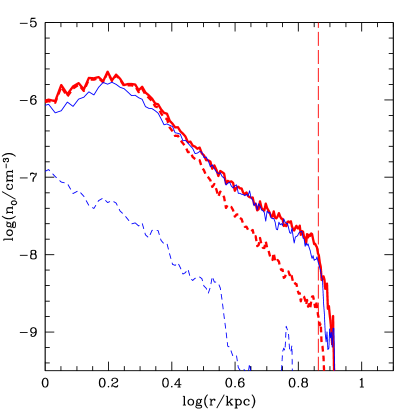
Figure 1: The radial density profiles of all oxygen (solid) and neutral oxygen (dashed) in halos of mass $10^{9.5}M_{\odot}$ in simulations without (blue) and with (red) self-shielding. Gas associated with galaxies has been removed. The right vertical dashed segment indicates the virial radius. Self-shielding enhances the neutral oxygen abundance significantly at all radii.

Having introduced our simulations, we are now in a position to demonstrate the importance of self-shielding. We compare in Figure 1 the mean radial density profiles of all oxygen (solid) and neutral oxygen (dashed) in simulations without (light blue) and with (heavy red) self-shielding (the r6n256wWwRT and r6n256wWwRT16d simulations, respectively). We produce these curves by averaging over halos in bins of mass and radius; see Section 3.2 for details. The solid curves overlap, indicating that simulations with similar reionization histories and identical models for galactic outflows yield similar metal density profiles. By contrast, the light blue dashed curve lies nearly a factor of 10 below the heavy red dashed curve, indicating that the neutral oxygen abundance is artifically underestimated by a factor of $\sim 10$ if self-shielding is ignored. It is interesting to note that our previous simulations underpredicted the observed abundance of OI at $z=6$ by a factor of $\approx 15$ (Figure 11 of Oppenheimer et al. 2009), independent of whether the ionization state was modeled using a spatially homogeneous EUVB or a background dominated by the nearest galaxy. In that work, the offset was interpreted as evidence for a partially-neutral universe at $z=6$. By contrast, Figure 1 suggests that the disagreement may owe to the absence of self-shielding in that work. If so, then OI observations may indeed be consistent with a reionized universe at $z=6$, with the observed systems arising entirely in optically thick regions such as galaxies. Our new simulations enable us to explore this possibility.

3 Metal Enrichment and Ionization

3.1 The Competition Between Enrichment and Reionization

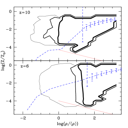
Figure 2: The relationship between metallicity, overdensity, neutral fraction, and reionization at $z=10$ (upper panel) and $z=6$ (lower panel). Blue dashed curves show the mean trend of metallicity versus overdensity while blue dashed error bars enclose the middle 50% wherever the median is nonzero. Light, medium, and heavy black contours represent neutral hydrogen fractions of $10^{-5}$, $10^{-2}$, and 0.5, respectively. The volume-averaged neutral fractions at $z=6$ and $z=10$ are 0.003 and 0.83, respectively. Red dotted curves indicate the minimum metal mass fraction to produce an observable absorber for a hydrostatically-bound region at $10^{4}$K.

Early interest in low-ionization metal absorbers centered on the possibility that the diffuse IGM could be enriched before it was reionized (Oh, 2002; Furlanetto & Loeb, 2003). The question of whether this works can be distilled to a competition between the growth of enriched regions and the growth of ionized regions. If galaxies reionize their environments more quickly than they enrich them, then OI absorption will be dominated by self-shielded clumps rather than by low-density regions that have not yet been reionized. On the other hand, if galactic outflows enrich the diffuse IGM (that is, regions with overdensity $\rho/\langle\rho\rangle<10$) very quickly, then there may be a substantial reservoir of neutral metals that can be observed in absorption prior to the completion of reionization. This idea seems unlikely at a glance because a galaxy’s ionization front ought to grow more rapidly than its metal pollution front. However, ionizing sources are not necessarily time-steady, and if star formation is bursty then the IGM surrounding a galaxy can recombine once its OB stars evolve off the main sequence. The metals ejected into the IGM are permanent, however, and could become visible in low-ionization transitions (Oh, 2002).

In order to motivate a detailed study of how this competition unfolds, we show in Figure 2 the relationship between overdensity, metallicity, and neutral hydrogen fraction before and after the completion of reionization. The blue dashed curves show the mass-weighted mean metal mass fraction as a function of overdensity. As was seen in Figure 4 of Oppenheimer et al. (2009), the mean metallicity grows significantly in regions that are moderately overdense ($\rho/\langle\rho\rangle<100$) while in denser regions it rapidly reaches an equilibrium value that is driven by self-regulated star-forming regions (Finlator & Davé, 2008). Importantly, outflows give rise to a reservoir of enriched gas at overdensities of 0.01–1 even at $z=10$. The red dotted curves show the minimum metal mass fraction for neutral regions in hydrostatic equilibrium at a temperature of $10^{4}$ K to produce an OI column greater than $10^{14}$cm^-2 as a function of overdensity. Comparing the red dotted and blue dashed curves indicates that overdense regions would produce observable absorption if they were homogeneously enriched to the mean level and neutral.

In order to ask whether the enriched regions could be neutral, we use contours to show the neutral hydrogen fraction as a function of density and metallicity. The heaviest or innermost contours illustrate the phase space where the neutral hydrogen fraction is $\geq 50\%$, hence they mark the transition from diffuse, ionized gas to condensed, neutral gas. The low-density limit of this region lies near the mean density at $z=10$, implying that much of the metal mass that is expelled into the IGM may remain neutral. Even at $z=6$, the bulk of the gas in the Lyman alpha forest ($\Delta\sim 10$) is on average neutral and enriched, implying the presence of a substantial forest of low-ionization metal absorbers.

Figure 2 seems to support the use of OI to probe the progress of reionization, but this could be misleading. The crucial question is whether the enriched regions are neutral and vice-versa. For example, a small population of enriched, ionized lumps could drive up the mean metallicity without suppressing the mean neutral fraction. To amplify this possibility, we use blue dashed error bars enclose the middle 50% of metallicities wherever the median metallicity is nonzero. They agree with the mean for overdensities above $\approx 30$, but at lower densities the median vanishes, indicating that the mean is driven by a small set of enriched regions. The need for detailed study of the IGM phase structure is further emphasized by observational evidence that metals mix quite poorly with the ambient IGM (Schaye et al., 2007). If the ionization state is similarly inhomogeneous, then the heavy averaging inherent in Figure 2 could be quite misleading. Our simulations model the inhomogeneous ionization and metallicity fields directly (subject to resolution limitations as described in Section 2.1), allowing us to address these questions.

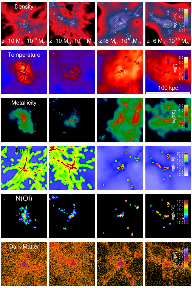
Figure 3: Maps of gas density, temperature, metallicity, HI column, OI column, and dark matter density for two halo masses at $z=10$ and $z=6$. Each panel spans 100 proper kpc, and the circles indicate the virial radii of the parent halos. At $z=10$, the weak EUVB leaves an abundant population of Lyman limit systems, but only those that lie near halos are associated with a significant OI column. By $z=6$, OI absorbers have retreated well into the central halo’s virial radius and are of generally higher column density.

In order to gain intuition into where OI absorbers live with respect to dark matter halos and LLSs, we show in Figure 3 maps of (top to bottom) gas density, temperature, metallicity, HI column, and OI column for four different dark matter halos at two different redshifts. The left two columns show how, at $z=10$, much of the volume is filled with neutral hydrogen as expected for a universe that is only 50% ionized. Near halos, this enriched gas produces OI columns stronger than $10^{14}$cm^-2 well outside of the virial radius. By $z=6$ the gas around similarly massive systems (right two columns) is even more enriched, but by now the ionization fronts have penetrated deeper into the halo, ionizing much of the diffuse gas that would have been visible as low-ionization absorbers at $z=10$. Countering this trend is the growing abundance of satellite halos, the cores of which are neutral and enriched. As a result, low-ionization absorbers are common around halos at both $z=10$ and $z=6$.

Figure 4: The characteristic column density for OI absorption as a function of overdensity in regions with nonzero metallicity. Contours enclose 67% and 99% of gas particles at $z=10$ (top) and $z=6$ (bottom). The dashed line indicates the 50% completeness limit (Becker et al., 2011). Regions with overdensities of less than 10 are never visible in absorption for $z<10$.

Figure 3 strongly suggests that OI absorbers trace enriched gas within dark matter halos rather than the diffuse IGM. A more quantitative way to ask which regions contain gas that is both enriched and neutral enough to yield observable absorption is to compute the characteristic column density as a function of density. If a parcel of gas is in hydrostatic equilibrium, then its characteristic OI column density $N_{\mathrm{OI},c}$ is

$$N_{\mathrm{OI},c}\equiv L_{J}\rho_{b}\frac{Z_{O}}{m_{O}}\frac{n_{OI}}{n_{O}}$$ (4)

where $L_{J}$ is the Jeans length, $\rho_{b}$ is the mass density in baryons, $Z_{O}$ is the mass fraction in oxygen, $m_{O}$ is the mass of an oxygen atom, and $n_{OI}/n_{O}$ is the neutral oxygen fraction (see Equations 3–4 of Schaye 2001). We compute the characteristic column density for each overdense particle using the local density, temperature, metallicity, and ionization state, and show the resulting trends at two representative redshifts in Figure 4. The dashed horizontal shows the current 50% observational completeness limit for selecting absorbers in OI (Becker et al., 2011). Gas at the mean density ($\rho/\langle\rho\rangle\sim 1$) is ionized by the nascent EUVB even at $z=10$, hence it does not produce observable OI absorption. While we cannot apply Equation 4 to underdense gas because it is not expected to be in hydrostatic equilibrium (Schaye, 2001), the trend in Figure 4 strongly suggests that it does not produce visible absorption either. At higher densities, the threshold for gas to be optically thick and hence neutral grows from $\approx 20$ at $z=10$ to $>300$ at $z=6$. Given that gas with overdensity greater than 10 is predicted to be enriched (Figure 2), the evolving threshold for it to be optically thick is also the threshold for it to produce visible OI absorption.

In summary, our simulations predict that ionization fronts precede metal pollution fronts, and that regions, once ionized, remain ionized. This owes partially to the fact that hydrogen-cooling halos produce stars steadily until their environments are reionized (note that Wise & Abel 2008 find that star formation becomes a steady-state process in pre-reionization halos more massive than $10^{7}M_{\odot}$, an order of magnitude below our resolution limit) and partially to the clustered nature of galaxy formation, although a detailed analysis of the relative roles of these factors is currently impossible owing to our small volumes. Consequently, diffuse gas does not produce observable absorption in low-ionization transitions. For the rest of this work, we will therefore focus on low-ionization metal absorption that occurs within dark matter halos.

3.2 Radial Profiles

In this Section, we explore how the radial density profiles of gas, total metals, and neutral metals vary with mass and redshift. We will consider halos that are both more and less massive than $10^{9}M_{\odot}$ because this marks the approximate threshold above which halos can accrete gas even in the presence of an EUVB. For consistency with Finlator et al. (2011b), we will refer to the lower-mass halos as “photosensitive” and the more massive halos as “photoresistant”.

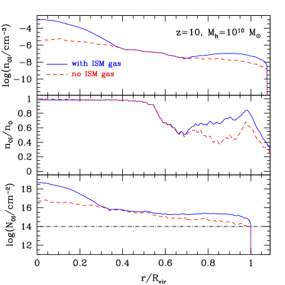
Figure 5: Sample profiles of OI density $n_{OI}$, neutral oxygen fraction $X_{OI}$, and neutral oxygen column density $N_{\mathrm{OI}}$ as a function of radius for the $10^{10}M_{\odot}$ central halo at $z=10$ shown in the left column of Figure 3. The solid blue profiles include both interstellar and intergalactic gas, while the dashed red profiles exclude all gas that is bound within resolved galaxies. The $n_{OI}$ and $X_{OI}$ profiles are both smoothed with a 1-kpc boxcar filter. The black dot-dashed curve in the bottom panel indicates current observational limits (Becker et al., 2011). We do not trace the profiles beyond a virial radius, hence they vanish there artificially. Excluding ISM gas suppresses the OI column at small radii owing to the central galaxy and at large radii owing to satellites, but on the whole the halo remains observable out to the virial radius.

We compute radial density profiles by stacking halos in bins of mass and averaging within each radial bin. By computing the density of OI within each shell directly (rather than computing the oxygen density and neutral fractions and multiplying them), we preserve small-scale inhomogeneities in the metallicity and enrichment fields.

As a demonstration of how our spherically-averaged radial profiling works, we show in Figure 5 the density, neutral fraction, and column density profiles for our most massive halo at $z=10$ (left colum in Figure 3). The solid blue curve shows that the halo possesses an enriched neutral core that is associated with OI column densities above $10^{16}$cm^-2 out to at least 0.2 virial radii ($R_{\rm vir}=6.6$kpc; bottom panel). This is dominated by star-forming gas in the central galaxy. Outside of this core there is an enriched, partially-neutral reservoir that generates observable column densities ($N_{\mathrm{OI}}>10^{14}$cm^-2; the black dot-dashed line in the bottom panel) out to the virial radius.

Our approach works well if the gas is distributed spherically-symmetrically, but it breaks down if the majority of a halo’s gas is bound into a small number of satellite systems because the geometric cross section for a sightline to intersect a satellite is smaller (and the associated gas column higher) than if the satellite’s gas were distributed in a shell. Additionally, the fact that our simulations neglect ionizations owing to the local radiation field means that the abundance of neutral oxygen within galaxies could be overestimated (we will return to this point in section 5). In order to mitigate these problems, we use SKID to identify and remove all gas that is associated with galaxies before computing density profiles. The dashed red curve shows the same density profile as the solid blue curve, but without galaxy gas. This step suppresses the density of neutral gas significantly near the halo’s core, but at larger radii the difference is slight because the gas in resolved satellites is subdominant to the combined contributions of unresolved satellites and the circumgalactic medium (CGM).

Note that the column densities in the bottom panel are notional because they are derived from spherically-averaged profiles. In the second part of this work, we will relax the assumption of spherical symmetry and use a ray-casting approach to compute the geometric absorption cross section, enabling a more accurate comparison with observations.

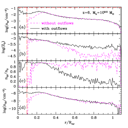
Figure 6: The radial profiles of hydrogen density, oxygen mass fraction, and neutral fraction, and neutral oxygen density in a $10^{9.5}M_{\odot}$ halo at $z=6$ in simulations without outflows (magenta dashed) and with outflows (black solid). The virial radius is 7.3 kpc. The red horizontal long-dashed line in the top panel indicates the threshold density for forming stars. The red vertical long-dashed line indicates the gravitational softening length. Outflows dominate the CGM at small radii and generate an atmosphere of ionized, enriched gas at large radii. They do not enhance the geometric cross section for absorption in low-ionization transitions.

Having demonstrated how we compute spherically-averaged profiles, we now ask how outflows impact the CGM. We show in Figure 6 the radial density profiles of gas and metals in $10^{9.5}M_{\odot}$ halos in simulations without (dashed magenta) and with (solid black) galactic outflows. Panel (a) compares the gas densities. The profiles flatten below one kpc because gas at these radii is dense enough to support star formation, which suppresses the gas density. Recalling that we have removed galactic gas from these profiles, we see that there is no circumgalactic gas within $0.1R_{\rm vir}$ unless outflows put it there because inflows at these radii collapse quickly onto the central galaxy. At larger radii, the profiles are nearly coincident because most of the gas is infalling rather than outflowing.

Panel (b) shows the oxygen metallicity profile. Near the central star-forming region (within 2 kpc), outflows give rise to an enriched atmosphere. At larger radii, simulations without outflows still suggest an enriched CGM. However, outflows clearly boost the mean metallicity beyond $0.2R_{\rm vir}$ (see also Oppenheimer et al., 2009).

We show the neutral oxygen fraction in panel (c). Nearly all of the CGM’s metals are neutral in the absence of outflows. These metals could correspond either to star-forming gas in satellite halos that are too small to be identified and removed by our group finder, or to moderately-enriched inflowing streams; simulations with higher resolution would be required to distinguish between these possibilities. By contrast, the neutral metal fraction drops at large radii in simulations with outflows. This does not owe to differences in the EUVB because $f_{\mathrm{esc}}$ is tuned separately for each simulation to produce similar EUVBs by $z=5$. Instead, it indicates that outflows tend to be highly ionized. A detailed analysis of the thermal structure of outflows is beyond the scope of the present work, but for reference we note that, for gas particles that have recently been ejected at $z=7$, our model predicts a median density of 0.4 times the mean baryon density and a median temperature of 30,000 K. For such gas, the recombination time exceeds a Hubble time, hence it is expected to be largely ionized by $z=7$.

The product of the curves in the top three panels is proportional to the neutral oxygen density, which we show in panel (d). This panel confirms that metals that are ejected in outflows are generally ionized and do not enhance the probability that the host halo will be observable as a low-ionization metal absorber. They must instead be sought using high-ionization transitions such as CIV (Oppenheimer & Davé, 2006; Borthakur et al., 2013) or OVI (Tumlinson et al., 2011). Note that this conclusion is not necesssarily general. For example, Ford et al. (2013) has shown that outflows enhance the abundance of MgII absorbers around $10^{12}M_{\odot}$ halos at low redshifts (their Figure 14).

Figure 7: The radial profiles of oxygen density in halos of mass $\log_{10}(M_{h}/M_{\odot})=8.3$ (panel a) and 9.5 (panel c) at $z=10$ in our fiducial simulation Panels (b) and (d) show the corresponding neutral fractions. Profiles are smoothed with a 0.3-kpc boxcar filter for clarity. At $z=10$, CGM metals are completely neutral in photosensitive halos and mostly neutral in photoresistant halos.

Figure 8: The same as Figure 8 but at $z=6$. We also distinguish total and neutral oxygen density in panels (a) and (c) as indicated. Once reionization completes, the EUVB penetrates to roughly $0.5R_{\rm vir}$ in both photosensitive and photoresistant halos. A tail of partially-neutral gas extends to the virial radius in the photoresistant halos, suggesting that they could dominate OI absorption statistics once reionization is complete.

In Figure 8, we evaluate how the OI density profile varies with mass prior to the completion of reionization. Examining the photosensitive halos first (panel a), we find that the central star-forming region ($<0.5R_{\rm vir}$) contains a significant reservoir of metals because these halos are massive enough to cool their gas and form stars. Furthermore, panel (b) shows that their metals remain completely neutral out to the virial radius because they inhabit preferentially underdense regions where the EUVB remains weak at $z=10$. We will show in Sections 4.1–4.3 that these halos have a geometric cross section to absorption that is not small compared to the halo cross section and that, consequently, they dominate OI absorption statistics prior to the completion of reionization.

Turning to photoresistant halos, we see that the density of metals is 1–2 orders of magnitude higher than in the photosensitive halos owing to their higher star formation efficiencies. The neutral fraction drops below unity outside of roughly $0.6R_{\rm vir}$ because these halos inhabit preferentially dense regions where the EUVB takes hold at earlier times. Even at the virial radius, however, the neutral fraction exceeds 50%, suggesting that these halos generate high-column absorbers even though they are subject to a stronger EUVB.

As the EUVB strengthens and ionization fronts penetrate the CGM, we expect the OI density profiles to evolve. We show in Figure 8 how the profiles in the same mass ranges have evolved by $z=6$ (note that the virial radii are also larger now). Photosensitive halos have grown a substantially higher total oxygen density, particularly near their cores ($\leq 0.3R_{\rm vir}$). These halos are able to continue forming new stars and metals even at $z=6$ owing to the fact that gas that cooled prior to reionization remains bound and star-forming for several dynamical times following overlap (Dijkstra et al., 2004). However, the gas is only neutral within $0.5R_{\rm vir}$. Gas at larger radii is completely ionized by the EUVB. In fact, our simulations suggest that halos near the hydrogen-cooling limit ($\sim 10^{8}M_{\odot}$) are evaporated by the EUVB in a process similar to the evaporation of minihalo gas (Shapiro et al., 2004). For both of these reasons, the abundance of neutral oxygen at the virial radius of photosensitive halos declines and their contribution to low-ionization metal absorbers diminishes as reionization proceeds.

Photoresistant halos are also more ionized than at $z=10$ (panels c and d), but the effect is weaker than for photosensitive halos. In detail, the fraction of neutral metals drops below 50% at roughly $0.5R_{\rm vir}$ in both cases, but the photoresistant halos are able to retain a significant component of neutral gas out to nearly the virial radius. Moreover, the total mass of circumgalactic metals around massive halos grows owing to continued star formation, metal expulsion, and possibly stripping of enriched gas from infalling satellites, as can clearly be seen in Figure 3. This means that, although photoresistant halos are exposed to a generally stronger EUVB, their denser CGM are able to attenuate the ionization fronts and preserve a reservoir of neutral metals that extends throughout much of the halo even at $z=6$.

In summary, Figures 8–8 suggest that the overall abundance of OI absorbers is regulated by a competition between the halo abundance, which grows in time, and absorption cross section, which declines for all halo masses as time progresses. All halos generate an enriched CGM down to the hydrogen cooling limit. The metals remain largely neutral at $z=10$ such that photosensitive halos are the predominant source of low-ionization metal absorbers prior to reionization. Nearer the epoch of overlap, photosensitive halos are completely ionized at radii larger than $0.5R_{\rm vir}$ whereas photoresistant halos are more than 10% neutral out to the virial radius. Hence the typical host halo mass of OI absorbers increases as reionization proceeds. We will quantify this evolution in Figures 10 and 12.

4 Modeling Observations

In this section we relate the properties of individual halos to volume-averaged statistical measurements of OI. Our analysis follows the approach adopted by many previous numerical studies of DLAs (for example, Katz et al., 1996). We begin by computing the geometric cross-section for halos to be observed in absorption in a way that relaxes the assumption of spherical symmetry. We then study how reionization affects the appearance of different halos in absorption. Finally, we apply our cross sections to predict the observable number density of absorbers and compare directly to observations.

4.1 Cross-section for Observability

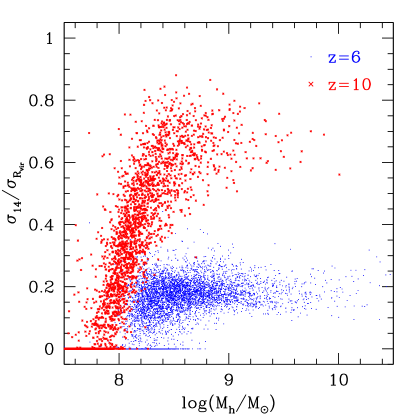
Figure 9: The fraction of the area within one virial radius $\pi R_{\rm vir}^{2}$ that is covered by lines of sight with a neutral oxygen column greater than $10^{14}$cm^-2 as a function of halo mass at $z=10$ (red crosses) and $z=6$ (blue points).

Halos that are more massive at a given redshift or at lower redshift for a given mass have produced more metals, leading to a higher cross section. Similarly, halos with lower mass at a given redshift should have a lower cross section both because they have produced fewer metals and because they are more susceptible to an EUVB. Our simulations allow us to quantify these effects with minimal assumptions. We begin by computing the geometric cross section for a halo to appear as an OI absorber with a column density greater than $10^{14}$cm^-2, which is the 50% completeness limit reported by Becker et al. (2011).

Computing the cross-sections accurately requires us to relax the assumption of spherical symmetry because the OI column density profiles are influenced by the filamentary structure of the gas density field (Figure 3). We map each of our halos onto a mesh with cells of width 200 physical parsecs including all gas out to twice the virial radius and then count the fraction of lines of sight passing within one virial radius for which the OI column density exceeds $10^{14}$cm^-2. We recompute this fraction using lines of sight in the x, y, and z-directions and average the three results. Using a finer mesh decreases the cross section while increasing the number of lines of sight with high columns, but the effect is weak; we have verified that using a mesh with twice this spatial resolution changes the cross-sections by $\sim 10\%$. Considering lines of sight that pass outside of one virial radius would primarily have the effect of picking up absorption owing to neighboring halos, as can be seen at $z=6$ in Figure 3. Incorporating the full three-dimensional gas distribution in this way automatically accounts for any departures from spherical symmetry. This means that, whereas we excluded gas that is closely associated with galaxies in Section 3.2 in order not to “smear” satellites over spherical shells when computing mean radial profiles, we include all halo gas in the analysis throughout the rest of this work.

We show in Figure 9 how the fraction of the area within one virial radius that is covered by observable lines of sight $\sigma_{14}/\sigma_{\rm vir}$ varies with halo mass at $z=10$ (red crosses) and $z=6$ (blue points). Broadly, $\sigma_{14}/\sigma_{\rm vir}<1$ even at $z=10$. In detail, halos more massive than $10^{8}M_{\odot}$ are generally visible throughout much of the virial radius because the EUVB has not yet penetrated deep into the CGM. Halos less massive than $10^{8}M_{\odot}$ show weaker absorption because they are not capable of producing stars and metals even in a neutral IGM. At $z=6$, the signature of reionization is obvious. The EUVB has penetrated well into the typical halo, suppressing the covered fraction to 10–30%. The threshold halo mass below which the absorption cross section vanishes grows from $10^{8}M_{\odot}$ at $z=10$ to roughly 2–3$\times 10^{8}M_{\odot}$ at $z=6$. This owes to the combined effects of photoionization and gas exhaustion on photosensitive halos.  Razoumov et al. (2006) used radiation hydrodynamic simulations to find that halos less massive than $7\times 10^{7}M_{\odot}$ retain the ability to accrete gas following reionization. Our simulations indicate a slightly higher threshold, likely owing to the tendency for outflows to reduce the gas density near halo cores. There is also a population of halos at both redshifts that produce no observable absorption ($\sigma_{14}=0$). This population extends to higher mass at $z=6$ than at $z=10$, indicating that it is not purely an artefact of limited mass resolution; instead, it reflects the weak star formation efficiencies and optically-thin CGM of photosensitive halos.

4.2 The Dominant Host Halos

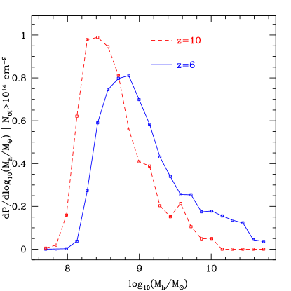
Figure 10: The probability density that the host halo of an OI absorber with column density greater than $10^{14}$cm^-2 has a given mass at $z=10$ and $z=6$. OI absorbers are dominated by halos a factor of 10–100 less massive than the halos that host Lyman break galaxies and Lyman-$\alpha$ emitters (Ouchi et al., 2010; Muñoz & Loeb, 2011).

As a first application of our cross sections, we may compute the most likely host halo mass for absorbers at a given column density. We do this by computing the probability density $P(M|N)$ that an absorber with column density $N_{\mathrm{OI}}>10^{14}$cm^-2 is hosted by a halo of mass $M<M_{h}<M+dM$ using Bayes’ theorem:

$$P(M|N)\propto P(N|M)P(M)$$ (5)

where $P(N|M)$ is the probability that a line of sight passing within the virial radius of a halo of mass $M$ encounters a column greater than $>10^{14}$cm^-2 and $P(M)$ is the prior probability of passing within a virial radius of a halo of mass $M$. The former is simply the ratio of the area within which the column exceeds $10^{14}$cm^-2 to the area within a virial radius (that is, $\sigma_{14}/\sigma_{\rm vir}$), and the latter is the fraction of halos in this mass range weighted by the area within a virial radius. We show this probability density at $z=6$ and $z=10$ in Figure 10.

At $z=10$, the distribution of halo masses that can host an observable system is weighted toward the hydrogen cooling limit partly because the enriched CGM in such halos remain mostly neutral, and partly because more massive halos are not yet abundant enough to compete. By $z=6$, the peak of the probability density function has shifted to higher mass by a factor of 2–3 because photosensitive halos lose their gas while photoresistant halos begin to assemble in force. Still, however, the characteristic host halo’s mass lies within the range that is sensitive to photoionization heating (Finlator et al., 2011b). This suggests that, at any redshift, low-ionization metal absorbers probe the lowest-mass halos that retain the ability to form stars.

How do the host halos of OI absorbers compare with the host halos of galaxies that are selected in emission?  Muñoz & Loeb (2011) used a detailed comparison between an analytic model and observations of Lyman break galaxies at $z=7$–8 to show that current observations likely do not probe below a halo mass of $\sim 10^{10}M_{\odot}$. Similarly, Ouchi et al. (2010) have used clustering observations to infer that Lyman-$\alpha$ emitters live in halos with masses between $10^{10}$–$10^{11}M_{\odot}$. Hence absorption-selected samples trace star formation in halos that are 10–100 times less massive than the halos that host emission-selected samples. This supports the suggestion by Becker et al. (2011) that studies in absorption offer more direct insight into the nature of the systems whose ionizing flux may have driven hydrogen reionization (see, for example Yan & Windhorst, 2004; Alvarez et al., 2012; Robertson et al., 2013).

Figure 10 also gives insight into what would be required to observe the host galaxies of OI absorbers in emission. The typical OI absorber at $z=6$ lives in a $10^{9}M_{\odot}$ halo. Our models predict that the mean star formation rate of such halos is 0.009$M_{\odot}\mbox{ yr}^{-1}$ (Finlator et al., 2011b). Assuming that the ratio of luminosity to SFR is $2\times 10^{28}$ ergs s^-1 Hz${}^{-1}(M_{\odot}\mbox{ yr}^{-1})^{-1}$ (Finlator et al., 2011a, note that this includes an estimate for dust extinction), this corresponds to a rest-frame ultraviolet absolute magnitude of -14. This is roughly three magnitudes fainter than has been achieved at $z\geq 6$ with the Hubble Space Telescope (Bouwens et al., 2012), and slightly fainter than will be achieved with the James Webb Space Telescope.

As a caveat to Figure 10, we note that the typical host halo mass at $z=6$ may be underestimated because the most massive halos are undersampled by our small simulation volume. In Figure 12, we will use an analytic fit to our results to extrapolate to higher masses and confirm that photosensitive halos still dominate.

4.3 The Contribution of Halos of Different Masses

4.3.1 Median Cross Section Versus Mass

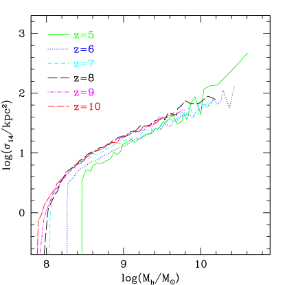
Figure 11: The median cross section for appearing as an absorber with an OI column density greater than $10^{14}$cm^-2 as a function of halo mass and redshift. The $z=5$ curve comes from our r6n256wWwRT16d simulation whereas the others all come from the r9n384wWwRT48d run. The minimum mass that can produce observable absorption and the proper cross section of massive halos both increase with declining redshift.

By how much does the cross section shrink from $z=10\rightarrow 6$? Figure 9 shows that the covered fraction declines at constant mass, but the x-axis is in units of virial radii. In practice, it is convenient to quantify the absorber abundance in terms of the number per absorption path length (section 4.3.2), which in turn depends on the cross section in proper units. To this end, we show in Figure 11 how the median cross section for observability $\sigma_{14}$ in proper kpc² depends on halo mass at 6 redshifts. The median trend evolves in three distinct ways. First, we still see a low-mass cutoff that grows owing to the gradual encroachment of ionization fronts into photosensitive halos. As before, the cutoff evolves from $<10^{8}M_{\odot}$ at $z=10$ to a few $\times 10^{8}M_{\odot}$ by $z=6$. Second, for halos with virial mass $<10^{10}M_{\odot}$, the growth of the EUVB dominates over the impact of continuing metal enrichment with the result that the cross section at a given halo mass shrinks. This is the signature of reionization: as observations probe higher redshifts, the EUVB weakens, halos are more neutral, and absorption shifts from high-ionization transitions in photoresistant halos to low-ionization transitions in photosensitive halos. This is consistent with the observation that the abundance of CIV absorbers declines at $z>6$ while the abundance of low-ionization systems does not (Becker et al., 2011). The shift to lower host halo masses may manifest as a decline in the characteristic velocity width as observations push past $z=5$; we will explore this possibility in future work. Finally, the cross section for photoresistant halos grows following $z=6$ (that is, the solid green curve lies above the dotted blue one for $z=5$ and $M_{h}/M_{\odot}>10^{9.5}$). This evolution is a direct response to our strongly redshift-dependent ionizing escape fraction (Section 2.1): If $f_{\mathrm{esc}}$ declines more rapidly than the star formation rate density increases, then the EUVB amplitude declines. As it does so, ionization fronts recede to larger halocentric radii, leaving more of the CGM neutral (since the recombination time remains much shorter than the Hubble time in moderately overdense gas at $z=6$). Whether this behavior is real depends on the true evolution of the EUVB. Current observations of the Lyman-$\alpha$ forest suggest that it strengthens dramatically from $z=6$ to $z=5$ (Bolton & Haehnelt, 2007; Kuhlen & Faucher-Giguère, 2012a) whereas it declines in our simulation, hence it may be no more than an artefact of our simple parameterization for $f_{\mathrm{esc}}$. It would be interesting to study how the cross section varies in a model that assumes a mass-dependent $f_{\mathrm{esc}}$ as such models may be able to reproduce the observed evolution of the EUVB more faithfully (for example, Alvarez et al. 2012; Yajima et al. 2011).

The evolution with redshift at the low-mass end may be compared with the finding by Becker et al. (2011) that the number density of low-ionization absorbers does not evolve strongly for $z>3$. In that work it was proposed that, at higher redshift, either the typical halo mass of absorbers decreases or the cross section for halos to appear as low-ionization absorbers increases. Figure 11 supports the idea that photosensitive halos, which are the predominant hosts of OI absorbers, do indeed have larger cross section in the presence of a weaker EUVB, in qualitative agreement with this scenario.

The trends in Figure 11 are well fit by a broken power law. We have performed a least-squares fit using the form $\log_{10}(\sigma_{14})=a+b\log_{10}(M_{h}/M_{\odot})$, where $\sigma_{14}$ is in proper kpc² and the fit parameters ($a$,$b$) change from ($a_{l},b_{l}$) to ($a_{h},b_{h}$) at the cutoff mass $\log_{10}(M_{h,c}/M_{\odot})$. Table 2 shows the resulting fits. The predicted power-law slope lies in the range 0.7–0.9, slightly steeper than what would be expected if the cross section for absorption were a constant fraction of each halo’s virial cross section ($M^{2/3}$). This indicates that feedback preferentially suppresses the OI abundance of low-mass systems. These slopes are consistent with the scalings that are found for absorption by neutral hydrogen (for example, Nagamine et al. (2004)), suggesting a physical correspondence between systems that are selected in OI and HI.

4.3.2 The Significance of Halos at Different Masses

It is convenient to quantify the number density of absorbers in terms of the number per absorption path length $l=dN/dX$, where the path length element $dX$ is defined in such a way that $l$ is constant if the comoving number density and proper cross section of the absorbers do not evolve (Bahcall & Peebles, 1969; Gardner et al., 1997):

$$dX\equiv(1+z)^{2}\frac{H_{0}}{H(z)}dz$$ (6)

The differential number density of absorbers per absorption path length per halo mass $M$ owing to absorbers with proper cross section $\sigma$ is:

$$\frac{dl}{dM}=\frac{c}{H_{0}}\sigma\frac{dn}{dM},$$ (7)

where $dn/dM$ is the dark matter halo mass function.

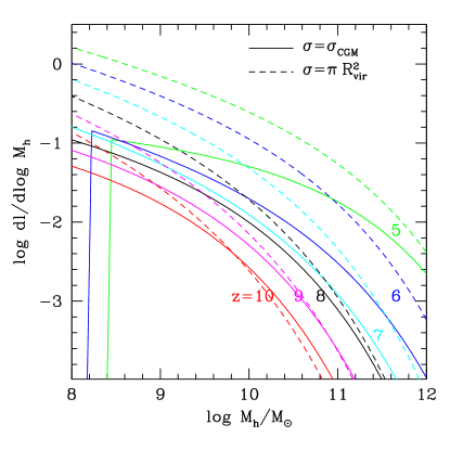
Figure 12: The differential contribution to the abundance of OI absorbers with column density greater than $10^{14}$cm^-2 as a function of mass and redshift. From bottom to top, curves correspond to $z=10,9,8,7,6$ and 5. Solid contours result from folding the predicted cross sections from the simulation directly into Equation 7 while dashed contours assume that the maximum observable radius is simply the virial radius.

In order to explore how halos of different masses contribute to the total abundance of observable (column density above $10^{14}$cm^-2) OI absorbers, we combine the analytical fits to our predicted cross sections in Table 2 with the Sheth & Tormen (1999) halo mass function using Equation 7 and show the resulting differential number counts from $z=10\rightarrow 5$ using solid curves in Figure 12. We consider only halos more massive than $10^{8}M_{\odot}$ as lower-mass halos tend to be unobservable (Figure 11). For comparison, we also show the predicted abundance under the assumption that each halo appears as an OI absorber out to its virial radius (dashed curves); we will refer to this as the “$R_{\rm vir}$ model”. Note that Figure 12 is qualitatively similar to Figure 10. The primary difference is that, while Figure 10 takes the full distribution of cross section as a function of halo mass into account, Figure 12 extrapolates to higher masses than can be explored in our simulations’ limited cosmological volumes.

The predicted abundance varies slowly from $z=10$ (lowest red curve) to $z=5$ (highest green curve) despite the onset of reionization at $z\sim 10$. At a given redshift, however, there is a cutoff mass (given by the final column in Table 2). Below this mass, the fractional contribution per unit halo mass vanishes, indicating that the rapid decline in cross section toward low masses cannot be made up by the increasing halo abundance. Above the cutoff mass, the curves approach the $R_{\rm vir}$ model because more massive halos are visible out to a larger fraction of the virial radius. However, the massive halos do not dominate absorbers by number because they are too rare. This confirms the conclusion from Figure 10 that photosensitive halos dominate observations even when the limitations of our small cosmological volume are corrected for.

4.4 Comparing to the Observed Number Density

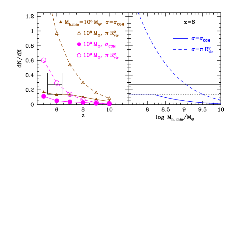
Figure 13: (left) The number density of absorbers with columns greater than $10^{14}$cm^-2 as a function of redshift. Filled brown triangles represent our predictions, which are marginally consistent with the observed 95% confidence interval of Becker et al. (2011) (box). Filled magenta circles use the same cross sections, but integrating only down to $10^{9}M_{\odot}$. Open triangles and circles indicate the $R_{\rm vir}$ model, integrated down to $10^{8}$ and $10^{9}M_{\odot}$, respectively. (right) The dependence of the predicted abundance at $z=6$ on a hypothetical low-mass cutoff in our simulations (solid ) and in the $R_{\rm vir}$ model (dashed). Horizontal lines indicate the observed 95% confidence interval.

By integrating Equation 7 over halo mass, we may compute the predicted number of absorbers per absorption path length. In the left panel of Figure 13, we compare the predicted and observed abundances as a function of redshift. The observations are from Becker et al. (2011), who identified nine OI absorbers along a total path length $\Delta X=39.5$ between $z=5.3$ and $z=6.4$. They estimate that, for systems with columns in excess of $10^{14}$cm^-2, their observations are 80–85% complete. Correcting for an assumed 85% completeness, we estimate an observed abundance of $0.27^{+0.16}_{-0.13}$ absorbers per path length with columns greater than $10^{14}$cm^-2, where the confidence intervals are 95% and account only for Poisson uncertainty.

The predicted absorber abundance (solid brown curve with filled triangles) is in marginal agreement with the observational $2\sigma$ confidence range. This level of consistency is remarkable given that the simulation has been calibrated using observations of high-ionization metal absorbers at lower redshifts (Oppenheimer & Davé, 2006) and tracers of hydrogen reionization (Section 2.1). The implication is that low-ionization metal absorbers are complementary probes of the same physical processes.

In detail, the predicted abundance of OI absorbers lies just below the observed 2$\sigma$ confidence intervals at $z\approx 6$ (open box). At this point, it is interesting to recall that our simulations also slightly overpredict the amplitude of the EUVB at $z=6$ (Section 2.2). These inconsistencies are probably telling the same story: At $z=6$, the simulated EUVB is too strong, yielding an optical depth to Lyman-$\alpha$ absorption that is too low. For the same reason, the simulated ionization fronts penetrate too far into halos, yielding geometric cross sections for low-ionization absorption that are too small, hence the predicted abundance of neutral metals is also low.

An additional source of uncertainty is the assumed metal yields: For reasonable choices of initial mass function and Type II supernova yields, the total oxygen yield can vary by a factor of 2–3. Doubling the assumed oxygen yield would not violate constraints on the $N_{\mathrm{OI}}/N_{\mathrm{HI}}$ ratio (Figure 14), but it would boost the predicted cross sections into improved agreement with observations.

The abundance is predicted to evolve quite slowly owing to cancellation between the growing abundance of halos and their declining geometric cross sections. If this evolution continues to lower redshifts, then it readily explains the slow evolution in the observed abundance of low-ionization absorbers between $z=6$ and $z=3$ (Becker et al., 2011).

Our simulations could underestimate the rate at which gas is expelled from photosensitive halos owing to incorrect outflow scalings or an improper treatment of the radiation field on small scales (see below), hence we recompute the abundance omitting halos less massive than $10^{9}M_{\odot}$ and show the result using filled magenta circles. This toy model lies well below observations, confirming that further suppression of star formation in photosensitive halos cannot be accommodated by existing data unless the EUVB is significantly weaker. As there is nothing special about $10^{9}M_{\odot}$, we show in the right panel the predicted abundance at $z=6$ as a function of the cutoff mass (solid blue curve); this figure confirms that the true cutoff mass cannot be much higher than $10^{8.5}M_{\odot}$ at $z=6$. Open triangles in the left panel show the $R_{\rm vir}$ model using halos more massive than $10^{8}M_{\odot}$. This comparison shows that absorption in $10^{8}M_{\odot}$ halos cannot extend out to the virial radius at $z=6$, and our simulations provide a self-consistent model for how this occurs. Open circles show the $R_{\rm vir}$ model assuming that halos below $10^{9}M_{\odot}$ do not contribute at all. This model is consistent with observations at $z=6$, suggesting that $10^{9}M_{\odot}$ halos host OI absorbers. Within our simulations, this is in fact the dominant mass scale (Figure 10). It falls below the simulated abundance at $z>7$, indicating the growing role that photosensitive halos may play at higher redshifts.

In summary, weighting the dark matter halo mass function by analytic fits to the predicted median trend of cross section versus halo mass confirms that OI absorption is dominated by the lowest-mass halos that sustain star formation at any redshift. The predicted absorber abundance evolves slowly owing to strong cancellation between the growing halo abundance and the declining cross section at a given mass, and it is in marginal agreement with observations at $z=6$. In detail, however, the predicted abundance is slightly low, consistent with the fact that the amplitude of the predicted EUVB is slightly too high.

4.5 Overlap with Neutral Hydrogen Absorbers

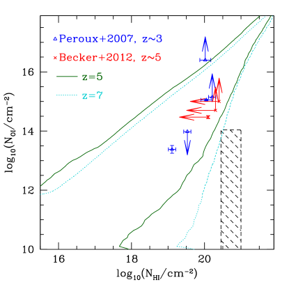
Figure 14: The dependence of neutral oxygen column density on the neutral hydrogen column density along lines of sight that pass through halos at $z=7$ (dotted turquoise) and $z=5$ (solid green). Contours enclose 99% of all sightlines. Metal absorbers with column densities $\log_{10}(N_{\mathrm{OI}})\geq 14$ correspond to neutral hydrogen columns of $\log_{10}(N_{\mathrm{HI}})=17-21.5$. Blue triangles are HI-selected absorbers at $z\sim 3$ (Péroux et al., 2007) while red crosses correspond to $z\sim 5$ Becker et al. (2012). The overlap with the predicted abundance ratios indicates agreement between predicted and observed metallicities. The shaded region shows the metallicity constraints on the foreground absorber in front of ULASJ1120+0641 under the assumption that it is gravitationally bound (Simcoe et al., 2012). Halo gas is already too enriched at $z=7$ to satisfy these constraints, suggesting that the absorber lies in the diffuse IGM.

The conclusion that low-ionization metal absorbers correspond to bound gas raises the question of how they relate to more familiar absorption-selected populations at lower redshifts. In particular, Becker et al. (2011, 2012) suggested that low-ionization metal absorbers could be analogous to DLAs and sub-DLAs. In order to consider this possibility, we project halos onto a grid with cells 100 physical pc wide (which is roughly the gravitational softening length) and pass sightlines through each pixel that falls within one virial radius in order to compute the neutral hydrogen and oxygen columns. We grid each halo in the x, y, and z directions independently in order to account for departures from spherical symmetry. We show how the $N_{\mathrm{OI}}$ and $N_{\mathrm{HI}}$ columns compare in Figure 14. Contours enclose 99% of all sightlines.

At $z=7$, observable OI absorption ($N_{\mathrm{OI}}>10^{14}$cm^-2) can arise in systems with neutral hydrogen columns of $10^{18}$–$10^{21}$cm^-2. By $z=5$, ongoing metal enrichment boosts the typical $N_{\mathrm{OI}}$ as a function of $N_{\mathrm{HI}}$ so that OI absorbers can be found in weaker systems. Additionally, the population of absorbers with relatively low metal columns (that is, the “tail” to low $N_{\mathrm{OI}}/N_{\mathrm{HI}}$) contracts, reflecting rapid enrichment of moderately overdense gas owing to low-mass systems.

Becker et al. (2012) have measured the OI and HI column for three low-ionization systems at $z\sim 5$; we include results from their Table 2 using red crosses. The overlap with the predicted abundance ratios at $z=5$ is excellent, indicating that the simulated metallicities are reasonable.

In order to emphasize the identification between OI-selected systems in our simulations and HI-selected systems from observations at lower redshifts, we also include OI constraints on DLAs and sub-DLAs at $z\sim 3$ from Péroux et al. (2007) (blue triangles). These measurements span the predicted range at $z=5$, suggesting that the evolution in the metal mass fraction at given HI column is comparable to the scatter at fixed redshift. Unfortunately, we cannot compare predictions and observations of HI-selected systems (note that the Becker et al. 2012 systems are selected as metal absorbers) directly because we have not evolved our simulations past $z=5$. Nevertheless, Figure 14 clearly supports the suggestion by Becker et al. (2012) that systems selected in low-ionization metal transitions are physically analogous to HI-selected systems.

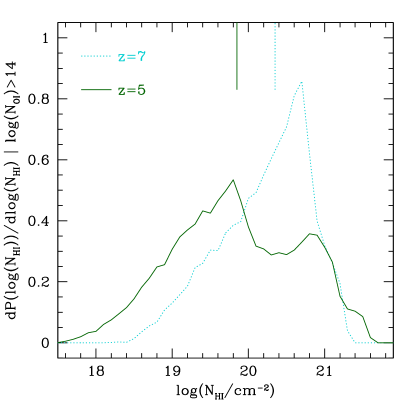
Figure 15: The distribution of neutral hydrogen columns for low-ionization metal absorbers with column densities in excess of $10^{14}$cm^-2 at $z=7$ (dotted turquoise) and $z=5$ (solid green). Vertical segments indicate the median $N_{\mathrm{HI}}$. Low-ionization metal absorbers receive significant contributions from DLAs and sub-DLAs, with a tail extending to LLS columns by $z=5$.

By selecting only systems with $N_{\mathrm{OI}}>10^{14}$cm^-2, we may ask directly what the predicted distribution of neutral hydrogen columns of low-ionization metal absorbers is. We show these probability distribution functions at $z=7$ (from our fiducial simulation) and $z=5$ (from the r6n256wWwRT16d simulation, which has the same physical treatments but subtends $(6/9)^{3}\approx 0.3$ times the cosmological volume) in Figure 15. The vertical segment shows the median $N_{\mathrm{HI}}$. At $z=7$, roughly half of OI absorbers are DLAs while half are sub-DLAs. By $z=5$, the fractional contribution from DLAs with $N_{\mathrm{HI}}\sim 10^{21}$cm^-2 remains unchanged. Meanwhile, ongoing enrichment boosts the neutral metal columns of systems $N_{\mathrm{HI}}<10^{20}$cm^-2. This suppresses the median $N_{\mathrm{HI}}$ of metal-selected samples into the sub-DLA range. Unfortunately, the doubly-peaked probability distribution function at $z=5$ indicates that our predictions suffer from volume limitations. Broadly, however, the conclusion is clear: Systems that are selected to have $N_{\mathrm{OI}}>10^{14}$cm^-2 are drawn with roughly equal probability from DLAs and sub-DLAs, with a slight evolution to lower hydrogen columns at lower redshifts owing to ongoing enrichment. Note that the distribution at $z=5$ as well its inverse, $N_{\mathrm{OI}}(N_{\mathrm{HI}})$ are predictions that may be tested directly.

Figure 14 also suggests that the overall number of detected systems increases for lower threshold column densities. This is not surprising; Oppenheimer et al. (2009) predicted that the column density distribution $d^{2}N/dXdN$ for low-ionization metals varies with $N$ as $N^{\alpha}$, where $\alpha$ falls between -1 and -2. While a detailed discussion of the predicted OI column density distribution is beyond the scope of the current work, we have recomputed the number of absorbers per path length $dN/dX$ for different threshold column densities using only the halos that occur in our fiducial simulation at $z=6$ (that is, there is no correction for more massive halos that are undersampled owing to volume limitations). Taking the ratio with respect to the $dN/dX$ for systems with $N_{\mathrm{OI}}>10^{14}$ cm^-2, we find relative abundances of 1.3, 1.1, and 0.8 for systems with $N_{\mathrm{OI}}$/cm^-2 $>10^{13}$, $5\times 10^{13}$, and $5\times 10^{14}$, respectively. Hence we expect a modest increase in the overall number of systems identified as survey sensitivity limits improve.

4.6 Foreground Absorption in ULAS J1120+0641

The $z=7.085$ quasar ULASJ1120+0641, reported by Mortlock et al. (2011), shows strong foreground absorption that could owe either to gas that lies within the quasar’s host galaxy, to an unassociated gravitationally-bound system analogous to DLAs that lies in the foreground, or to a neutral patch of the IGM that happens to lie along the line of sight. Recently, Simcoe et al. (2012) used a high-resolution infrared spectrum to search for metal absorption at the position of the foreground absorber. The detection of metal absorption would give strong support to the view that it corresponds to a discrete system rather than to the diffuse IGM. They estimated a foreground neutral hydrogen column of $\log_{10}(N_{\mathrm{HI}}/\mathrm{cm}^{-2})=$20.45–21.0. They did not detect any metal absorption at the redshift of the absorber (with the exception of a 2.2$\sigma$ detection of neutral oxygen). Modeling their upper limits under the assumption that the absorber was discrete, they found that the OI column density was constrained to be less than $14.04$ cm^-2 at $2\sigma$.

We may use our simulated sightlines to ask whether these measurements are consistent with arising in halo gas. To this end, we compare in Figure 14 the predicted distribution of OI and HI columns at $z=7$ (cyan contours) with the observationally-allowed combinations (shaded region). Given that 1% of simulated sightlines lie outside of the cyan region, it is clear at a glance that there is negligible overlap between the predicted column density ratios of halo gas and the Simcoe et al. (2012) constraints. For completeness, however, we may estimate the predicted probability that the observed absorption does arise in halo gas as follows: The redshift of the absorber is constrained to be $7.041\pm 0.003$, corresponding to a 3-$\sigma$ observed path length of 0.79 Mpc. Neglecting shadowing and including sightlines in the x, y, and z directions, our simulations effectively model a path length of $3.06\times 10^{8}$ Mpc and identify 34,090 absorbers that satisfy the Simcoe et al. (2012) constraints. Hence the model predicts that the probability of encountering a system satisfying the Simcoe et al. (2012) constraints over the observed path length is $\sim 10^{-4}$. We conclude that the foreground absorber is not consistent with arising in halos because bound gas at the inferred HI column is already too enriched at $z=7$.

If the foreground absorption does not arise in a halo, then it must arise in the diffuse IGM. In this case, Simcoe et al. (2012) find that the metal mass fraction must be less than $10^{-3}$ in solar units. In our simulations, the mean metallicity at $z=7$ falls below this limit for all gas that is less dense than 0.3 times the mean density. In other words, a typical underdense region readily satisfies the observational constraints.

We may also consider under what conditions the foreground absorption could originate in bound gas without matching the OI column densities expected from our simulations. The class of simulations presented here yields reasonable agreement with a wide range of observational constraints including the galaxy mass-metallicity relation at $z=2$ (Finlator & Davé, 2008), the abundance of CIV absorbers at $z=6$ (Oppenheimer et al., 2009), the rest-frame ultraviolet luminosity function of galaxies (Davé et al., 2006; Oppenheimer et al., 2009; Finlator et al., 2011b), and the history of reionization (Section 2.2 and Finlator et al. 2012). Thus, we expect the OI column densities to be a robust prediction. Nonetheless, the foreground absorption could still originate in bound gas if the true star formation rate density per unit gas density $\dot{\rho}_{*}/\rho_{g}$ is lower than assumed in our models. In this case, gas could remain unenriched until it reaches much higher columns than $N_{\mathrm{HI}}=20.5$ cm^-2. A dependence of $\dot{\rho}_{*}/\rho_{g}$ on metallicity is in fact expected theoretically (Gnedin & Kravtsov, 2010), and implementations of this idea within numerical simulations generically predict suppressed star formation rates in low-mass halos (Kuhlen et al., 2012b; Thompson et al., 2013). We will return to these models in Section 5; for now, we note that this possibility motivates future work comparing the dependence of metallicity on density in simulations that assume different star formation and feedback models.

In summary, the stringent limits on the metal abundance of the absorbing gas are not satisfied by overdense gas in our simulations. Meanwhile, they are readily satisfied by underdense gas at $z\geq 7$. Given the level of realism implied by the range of observational constraints that our simulations are known to satisfy, these comparisons argue that the intervening gas lies in the diffuse IGM rather than in a discrete absorber. This implies a volume-averaged neutral hydrogen fraction of $\sim 10\%$ at $z=7$ (Bolton et al., 2011; Schroeder et al., 2013).

5 Discussion

5.1 Implications

The agreement between the predicted and observed abundances of OI absorbers in Figure 13 is consistent with a scenario in which star formation persists at scales a factor of 10–100 lower in mass than is currently probed by observations of galaxies in emission (Muñoz & Loeb, 2011; Ouchi et al., 2010). If true, then the abundance of OI absorption systems places a strong constraint on models in which star formation in low-mass halos is suppressed owing to, for example, inefficient formation of molecular clouds at low metallicities (Krumholz & Dekel, 2012; Kuhlen et al., 2012b; Christensen et al., 2012; Thompson et al., 2013) or a mass threshold below which gas accretion ceases (Bouché et al., 2010).

At the same time, the abundance of neutral oxygen must be suppressed in halos roughly a factor of 10 more massive than the hydrogen cooling limit by $z=6$ or else the abundance of OI absorbers would be substantially overproduced (brown dashed curve with open triangles). Given that such systems readily form stars (Finlator et al., 2011b) and enrich their CGM prior to the onset of reionization (Figure 8), this indicates that their CGM must be substantially ionized at $z=6$.

As an alternative to this picture, it is possible that star formation is inefficient in halos much more massive than $10^{9}M_{\odot}$ as long as the cross-section for more massive halos to appear as OI absorbers significantly exceeds their virial radius. For example, Kuhlen et al. (2012b) have shown that a model in which stars form only out of molecular gas suppresses star formation in halos less massive than $10^{10}M_{\odot}$ at $z\geq 4$. If true, this model would imply that OI absorbers are associated with larger halos than predicted by our simulations. They could not be arbitrarily large, however: The velocity widths reported by Becker et al. (2011) are narrower than would be expected for gas associated with $10^{11}M_{\odot}$ halos, with five out of seven systems exhibiting velocity widths of less than $100\;{\rm km}\,{\rm s}^{-1}$.

We disfavor this option for two reasons. First, the model discussed by Kuhlen et al. (2012b) may be too efficient at suppressing star formation in low-mass galaxies. For example, it underproduces the abundance of faint UV-selected galaxies at $z=4$ (see the KMT07 curve in Figure 18). Similarly, recent observations suggest that the UV luminosity function rises to -13 at $z=2.4$ (Alavi et al., 2013), in conflict with predictions from metallicity-dependent cooling models (Kuhlen et al., 2013). The results of Alavi et al. (2013) are based on only a few objects, but if verified in future work then they indicate that star formation continues in halos less massive than $10^{10}M_{\odot}$, in agreement with our predictions.

These discrepancies may be removed by increasing the mass resolution (Figure 16 of Kuhlen et al., 2012b) or changing the numerical implementation (for example, Jaacks et al., 2013; Thompson et al., 2013), although in all of these models the predicted UV luminosity function turns over at a luminosity is too bright to match the Alavi et al. (2013) results. Increasing the efficiency of star formation in low-mass systems sufficiently to reproduce the abundance of faint UV-selected galaxies would decrease the halo mass below which star formation is suppressed, bringing these models back into agreement with ours.

More broadly, the assumption that reionization was driven by galaxies already leads naturally to the conclusion that star formation must continue to scales at least $100\times$ fainter than current limits. This idea is further supported both by considerations regarding the number of ionization photons that can be provided by observed galaxies (Robertson et al., 2013; Calvi et al., 2013) as well as the fraction of gamma-ray bursts with no optical counterpart (Trenti et al., 2012). The view that OI absorption directly probes this population is more natural.

The second difficulty with models attributing OI absorbers to halos more massive than $10^{10}M_{\odot}$ is that it is difficult to understand how an optically-thick, enriched CGM would extend with large cross-section to such large distances around massive halos given that they are expected to live in regions where the EUVB is more intense. Even at $z=10$, halos are not completely optically thick in our simulations (Figure 9), hence it is not likely that a significant absorption column exists well outside the virial radius.

The idea that OI absorbers originate in low-mass halos raises the possibility of using absorbers, Lyman break galaxies, and Lyman-$\alpha$ emitters jointly to constrain how star formation and feedback scale with halo mass across a much wider range of halo masses than can be probed by any population alone. Such an inquiry would require an improved understanding of the connection between a halo’s star formation rate and its cross section for observability in absorption, a daunting undertaking both for theory and for observation (Fynbo et al., 2008; Krogager et al., 2013). However, the reward would be a powerful probe of star formation and feedback across many decades of dynamic range.

Our simulations predict that the overall abundance of OI absorbers increases slowly in time, particularly below $z=6$. It should be possible to test this prediction with existing observations, although existing catalogs of absorbers tend to be pre-selected as DLAs rather than as OI absorbers; the overlap between these two populations would require improved understanding in order to correct for selection biases.

5.2 Limitations

Our simulations suffer from several limitations associated with resolution and numerical methodology. First, they resolve halos at the hydrogen cooling limit with $\sim 100$ particles. While this is sufficient for a converged mass density profile (Trenti et al., 2010), it is not clear that this criterion also leads to a converged absorption cross-section. To explore this, we compared the absorption cross-section for two simulations with different mass resolutions. These simulations, the r3wWwRT32 and r6wWwRT32 simulations from Finlator et al. (2011b), use $2\times 256^{3}$ particles to model 3 and $6h^{-1}{\rm Mpc}$ volumes, respectively. In contrast to our more recent simulations, they adopt a constant $f_{\mathrm{esc}}=0.5$ and do not include a subgrid self-shielding prescription. To simulate self-shielding in post-processing, we therefore assume that all gas with baryon overdensity greater than 320 is fully neutral while less dense gas is fully ionized; this approximates the behavior of our more recent simulations at $z=$6–7. For halos more massive than $10^{9}M_{\odot}$, the cross sections in the high-resolution calculation are roughly 70% as large as at our fiducial resolution at $z=6$ and $z=7$. The difference owes to the explicit dependence of outflow properties on halo mass coupled with the fact that star formation begins sooner at higher mass resolution. Hence we estimate that mass resolution limitations affect the predicted abundance of absorbers at the $\sim 50\%$ level.

Second, our simulations do not treat the interaction between outflowing gas and the CGM correctly because outflows consist of isolated gas particles that are expelled at roughly the escape velocity from star-forming regions. Given that smoothed-particle hydrodynamics defines a particle’s thermal properties by smoothing over the properties of neighboring particles, this simplified treatment precludes the formation of multiphase outflows in which cold, optically thick cores are entrained in a hot, optically-thin medium. The lack of a cold component embedded in the outflows could in turn lead us to underestimate the geometric cross section to absorption in low-ionization transitions. For similar reasons, our simulations probably do not treat the mixing that occurs between different phases in the CGM correctly. This effect may be crucial in reconciling models with the observed velocity width distribution of DLAs (Tescari et al., 2009).

Third, our simulations are known to treat shocks and hydrodynamic instabilities inaccurately, leading to unphysical behavior at fluid boundaries.  Bird et al. (2013) have compared the $f(N_{\mathrm{HI}})$ predictions in simulations using smoothed particle hydrodynamics versus a new moving-mesh formalism, arepo, that alleviates many of these issues. arepo predicts that absorbers with $N_{\mathrm{HI}}=10^{19}$–$10^{20}$ are more abundant than in gadget whereas absorbers with $N_{\mathrm{HI}}=10^{20}$–$10^{21}$ are less abundant. Coincidentally, our simulations predict that OI absorbers fall with roughly equal probability into these two ranges (Figure 15), hence the overall impact on the predicted OI absorber population is difficult to predict. Moreover, their calculations did not include a treatment for galactic outflows, which can significantly impact absorption statistics (Nagamine et al., 2007; Tescari et al., 2009). A more complete appraisal of the impact of hydrodynamic instabilities will therefore require further work.

Fourth, our model neglects ionizations that occur within halos owing to nearby stars. This is because it attenuates the radiation field on scales smaller than the radiation transfer grid using a subgrid self-shielding approach. Implicitly, our simulations assume that a fraction $1-f_{\mathrm{esc}}$ of ionizing photons are absorbed by molecular clouds that behave as photon sinks while the other $f_{\mathrm{esc}}$ escape through optically-thin holes directly into the IGM, where the mean free path is large enough to be resolved by our radiation transport solver. This yields a purely outside-in reionization topology (Miralda-Escudé et al., 2000) in which gas that is more dense than an evolving threshold density is completely neutral. Analytic estimates suggest that local ionizations could suppress the abundance of neutral hydrogen absorbers with columns greater than $10^{17}$cm^-2 (Miralda-Escudé, 2005; Schaye, 2006) at $z=3$, which in our model includes all observable OI absorbers (Figure 15). Indeed, the local field could be even more important at $z\geq 6$, when the EUVB is much weaker.

While a detailed calculation of the local field is beyond the scope of our current work, it is useful to consider the implications of recent studies.   Nagamine et al. (2004, 2007) used a subgrid prescription for the multiphase ISM (Springel & Hernquist, 2003) to model the ISM neutral fraction and found that the abundance of neutral hydrogen absorbers $f(N_{\mathrm{HI}})$ with columns $N_{\mathrm{HI}}<10^{21}$cm^-2 at $z=3$ was underproduced; this suggested that dense gas was overionized.  Tescari et al. (2009) reproduced their result using a similar prescription and found that, by assuming that all gas more dense than a threshold of 0.01cm^-3 was neutral, they could increase the predicted DLA abundance by 0.2 dex.  Nagamine et al. (2010) confirmed that invoking a slightly lower density threshold ($6\times 10^{-3}$cm^-3) yielded excellent agreement with observations across a wide range of $N_{\mathrm{HI}}$.  Pontzen et al. (2008), McQuinn et al. (2011), and Yajima et al. (2012), used radiation transport calculations to calculate the threshold density and found excellent agreement with the observed $f(N_{\mathrm{HI}})$. These works indicate that the local field must be modest within the halos that dominate $f(N_{\mathrm{HI}})$ at $z=3$.

At the factor-of-two level, however, it cannot be ignored.  Yajima et al. (2012) found that the local radiation field reduces the geometric absorption cross section for $10^{9}M_{\odot}$ halos by $\approx 50\%$ at $z=3$.  Rahmati et al. (2013) found that the local field suppresses the abundance of systems with $N_{\mathrm{HI}}=10^{19}$–$10^{21}$cm^-2 by a factor of 3 at $z=5$. Importantly, they also noted that the role of the local field is quite sensitive to the uncertain relative spatial distribution of sources and sinks within the ISM. Finally, Fumagalli et al. (2011) found that the local background reduces the cross section by no more than $50\%$ for absorbers with columns $N_{\mathrm{HI}}=10^{18}$–$10^{21}$cm^-2 (their Figure A1). These studies, many of which incorporate much higher resolution than ours, suggest that the local field can suppress $f(N_{\mathrm{HI}})$ by a factor of 2–3. Given the tight coupling between the hydrogen and oxygen neutral fractions, we conclude that it could likewise suppress the OI cross sections by a factor of 2–3. This crude estimate neglects the role of radial metallicity gradients, but it indicates that uncertainties associated with the local field are not large compared to uncertainties associated with the limited observational sample size. On the other hand, the local field’s significance may be comparable to the amount by which cross sections shrink owing to the strengthening EUVB (Figure 11).

Another consequence of the local ionizing background could be to modulate the dominant mass scale of OI absorbers’ host halos. In particular, if $f_{\mathrm{esc}}$ increases to low halo masses (Alvarez et al., 2012; Yajima et al., 2011), then it could suppress the absorption cross-section in halos less massive than $10^{9}M_{\odot}$. In order not to compromise the good agreement between the predicted and observed abundance of absorbers (Figure 13), a small decrease in the cross-section of low-mass halos would have to be compensated by a large increase in halos with masses in the range $10^{9}$–$10^{11}M_{\odot}$ (more massive host halos would be difficult to reconcile with the velocity widths reported by Becker et al. 2011), but this does not seem impossible. We conclude that, while our simulations represent a plausible model for low-ionization absorbers, the local ionizing background remains a source of uncertainty regarding the nature of their host population.

Finally, our model for galactic outflows may not incorporate the correct scaling between outflow mass loading factors, velocities, and host galaxy properties. This is important because the properties of DLAs are sensitive to outflows (Nagamine et al., 2007; Tescari et al., 2009). It has recently been shown that an alternative model in which low-mass galaxies eject more mass per unit stellar mass formed than in the current model produces improved agreement with the observed mass function of neutral hydrogen (Davé et al., 2013). This model may predict lower metallicity in dense gas, suppressing the abundance of low-ionization metal absorbers at high column densities. while enhancing the abundance of high-ionization absorbers.

In summary, mass resolution limitations may affect the predicted abundance of OI absorbers at the $\sim 50\%$ level; the local ionizing background could affect results at the $\sim$factor of 3 level; and the impact of uncertainties related to inaccuracies in our hydrodynamic solver, our treatment for galactic outflows, and $f_{\mathrm{esc}}$ is difficult to ascertain. None of these considerations challenges the basic prediction that OI absorbers are associated with gravitationally bound gas in systems that are analogous to DLAs and sub-DLAs at lower redshifts. Further work is required, however, in order to improve our understanding of the likely mass scale of their host halos.

6 Summary

We have used a cosmological radiation hydrodynamic simulation to study the nature of OI absorption in the reionization epoch. The diffuse IGM is not sufficiently enriched by $z=10$ for OI to trace its ionization state directly. Instead, OI is tightly associated with dense gas that lies within dark matter halos. In the absence of an EUVB, all halos more massive than the hydrogen cooling limit possess significant reservoirs of neutral oxygen out to a substantial fraction of the virial radius; in this case OI observations are dominated by halos near the hydrogen cooling limit. An EUVB ionizes and evaporates gas out of halos less massive than $\sim 10^{9}M_{\odot}$; such halos then become unobservable at their virial radius with the result that the characteristic host halo mass of low-ionization absorbers increases. This may cause the characteristic velocity widths to increase to lower redshifts. Even so, however, the dominant host halos of OI absorbers are not more massive than $10^{9}M_{\odot}$ at $z=6$. Hence OI absorbers trace the signatures of star formation in halos a factor of 10–100 less massive than the halos that host emission-selected samples such as Lyman break galaxies and Lyman-$\alpha$ emitters. Our simulations yield marginal agreement with the observed OI absorber abundance at $z\sim 6$. In detail, the predicted abundance is slightly low, consistent with the fact that the predicted EUVB is slightly too strong compared to constraints from the Lyman-$\alpha$ forest.

We additionally compare our density profiles to the upper limits on the OI column density of the absorber in the foreground of the $z=7.085$ quasar ULASJ1120+0641 and find that the limits cannot be satisfied by gas within halos because gas at the observed HI column density is already too enriched by $z=7$. By contrast, gas at less than one third the mean density has a low enough metallicity to satisfy the constraints at $z\geq 7$. This supports the view that the absorption occurs in the diffuse IGM rather than in a discrete system and argues for a $\sim 10\%$ volume-averaged neutral hydrogen fraction.

Table 1: Our simulations. The fiducial simulation is indicated in bold.

name	$L$	RT grid	outflows?	self-shielding?
r6n256wWwRT16d	6	$16^{3}$	yes	yes
r6n256nWwRT16d	6	$16^{3}$	no	yes
r9n384wWwRT48d	9	$\mathbf{48^{3}}$	yes	yes
r6n256wWwRT	6	$16^{3}$	yes	no

Table 2: Cross-section versus halo mass and redshift.

redshift	$a_{l}$	$b_{l}$	$a_{h}$	$b_{h}$	$\log_{10}(M_{h,c}/M_{\odot})$
5	-535.981	63.5	-6.8	0.875	8.45
6	-554.636	67.5	-5	0.675	8.225
7	-483.55	60.5	-4.95	0.675	8
8	-422.295	53	-6	0.8	7.975
9	-238.141	30	-6.2	0.825	7.95
10	-236.74	30	-6.85	0.9	7.9

References

- National Academies Press (2010) National Research Council. New Worlds, New Horizons in Astronomy and Astrophysics. Washington, DC: The National Academies Press, 2010.
- Alavi et al. (2013) Alavi, A., Siana, B., Richard, J., et al. 2013, arXiv:1305.2413
- Alvarez et al. (2012) Alvarez, M. A., Finlator, K., & Trenti, M. 2012, ApJL, 759, L38
- Bahcall & Peebles (1969) Bahcall, J. N., & Peebles, P. J. E. 1969, ApJL, 156, L7
- Barkana & Loeb (2004) Barkana, R., & Loeb, A. 2004, ApJ, 609, 474
- Becker et al. (2011) Becker, G. D., Sargent, W. L. W., Rauch, M., & Calverley, A. P. 2011, ApJ, 735, 93
- Becker et al. (2012) Becker, G. D., Sargent, W. L. W., Rauch, M., & Carswell, R. F. 2012, ApJ, 744, 91
- Bird et al. (2013) Bird, S., Vogelsberger, M., Sijacki, D., et al. 2013, MNRAS, 429, 3341
- Bolton & Haehnelt (2007) Bolton, J. S., & Haehnelt, M. G. 2007, MNRAS, 382, 325
- Bolton et al. (2011) Bolton, J. S., Haehnelt, M. G., Warren, S. J., et al. 2011, MNRAS, 416, L70
- Borthakur et al. (2013) Borthakur, S., Heckman, T., Strickland, D., Wild, V., & Schiminovich, D. 2013, ApJ, 768, 18
- Bouché et al. (2010) Bouché, N., Dekel, A., Genzel, R., et al. 2010, ApJ, 718, 1001
- Bouwens et al. (2012) Bouwens, R. J., Illingworth, G. D., Oesch, P. A., et al. 2012, ApJL, 752, L5
- Calvi et al. (2013) Calvi, V., Pizzella, A., Stiavelli, M., et al. 2013, MNRAS, 432, 3474
- Christensen et al. (2012) Christensen, C., Quinn, T., Governato, F., et al. 2012, MNRAS, 425, 3058
- Davé et al. (2006) Davé, R., Finlator, K., & Oppenheimer, B. D. 2006, MNRAS, 370, 273
- Davé et al. (2013) Davé, R., Katz, N., Oppenheimer, B. D., Kollmeier, J. A., & Weinberg, D. H. 2013, arXiv:1302.3631
- Dijkstra et al. (2004) Dijkstra, M., Haiman, Z., Rees, M. J., & Weinberg, D. H. 2004, ApJ, 601, 666
- Eisenstein & Hu (1999) Eisenstein, D. J., & Hu, W. 1999, ApJ, 511, 5
- Fan et al. (2002) Fan, X., Narayanan, V. K., Strauss, M. A., et al., Evolution of the Ionizing Background and the Epoch of Reionization from the Spectra of Quasars, 2002, AJ, 123, 1247
- Fan et al. (2006) Fan, X., Strauss, M. A., Becker, R. H., et al. 2006, AJ, 132, 117
- Finkelstein et al. (2012) Finkelstein, S. L., Papovich, C., Ryan, R. E., et al. 2012, ApJ, 758, 93
- Finlator & Davé (2008) Finlator, K., & Davé, R. 2008, MNRAS, 385, 2181
- Finlator et al. (2011a) Finlator, K., Oppenheimer, B. D., & Davé, R. 2011, MNRAS, 410, 1703
- Finlator et al. (2011b) Finlator, K., Davé, R., Özel, F. 2011, ApJ, 743, 169
- Finlator et al. (2012) Finlator, K., Oh, S. P. Özel, F., & Davé, R. 2012, MNRAS, in press
- Ford et al. (2013) Ford, A. B., Oppenheimer, B. D., Davé, R., et al. 2013, MNRAS, 1160
- Fumagalli et al. (2011) Fumagalli, M., Prochaska, J. X., Kasen, D., et al. 2011, MNRAS, 418, 1796
- Furlanetto & Loeb (2003) Furlanetto, S. R., & Loeb, A. 2003, ApJ, 588, 18
- Furlanetto et al. (2004a) Furlanetto, S. R., Zaldarriaga, M., & Hernquist, L. 2004, ApJ, 613, 1
- Furlanetto et al. (2004b) Furlanetto, S. R., Zaldarriaga, M., & Hernquist, L. 2004, ApJ, 613, 16
- Furlanetto & Oh (2005) Furlanetto, S. R., & Oh, S. P. 2005, MNRAS, 363, 1031
- Fynbo et al. (2008) Fynbo, J. P. U., Prochaska, J. X., Sommer-Larsen, J., Dessauges-Zavadsky, M.,
- Gardner et al. (1997) Gardner, J. P., Katz, N., Hernquist, L., & Weinberg, D. H. 1997, ApJ, 484, 31
- Gnedin & Fan (2006) Gnedin, N. Y., & Fan, X. 2006, ApJ, 648, 1
- Gnedin & Kravtsov (2010) Gnedin, N. Y., & Kravtsov, A. V. 2010, ApJ, 714, 287
- Haehnelt et al. (1998) Haehnelt, M. G., Steinmetz, M., & Rauch, M. 1998, ApJ, 495, 647
- Hinshaw et al. (2012) Hinshaw, G., Larson, D., Komatsu, E., et al. 2012, arXiv:1212.5226
- Jaacks et al. (2013) Jaacks, J., Thompson, R., & Nagamine, K. 2013, ApJ, 766, 94
- Katz et al. (1996) Katz, N., Weinberg, D. H., Hernquist, L., & Miralda-Escude, J. 1996, ApJL, 457, L57
- Komatsu et al. (2011) Komatsu, E., et al. 2011, ApJS, 192, 18
- Krogager et al. (2013) Krogager, J.-K., Fynbo, J. P. U., Ledoux, C., et al. 2013, MNRAS, 433, 3091
- Krumholz & Dekel (2012) Krumholz, M. R., & Dekel, A. 2012, ApJ, 753, 16
- Kuhlen & Faucher-Giguère (2012a) Kuhlen, M., & Faucher-Giguère, C.-A. 2012, MNRAS, 423, 862
- Kuhlen et al. (2012b) Kuhlen, M., Krumholz, M. R., Madau, P., Smith, B. D., & Wise, J. 2012, ApJ, 749, 36
- Kuhlen et al. (2013) Kuhlen, M., Madau, P., & Krumholz, M. 2013, arXiv:1305.5538
- McGreer et al. (2011) McGreer, I. D., Mesinger, A., & Fan, X. 2011, MNRAS, 415, 3237
- McQuinn et al. (2011) McQuinn, M., Oh, S. P., & Faucher-Giguère, C.-A. 2011, ApJ, 743, 82
- Mesinger (2010) Mesinger, A. 2010, MNRAS, 407, 1328
- Miralda-Escudé et al. (2000) Miralda-Escudé, J., Haehnelt, M., & Rees, M. J. 2000, ApJ, 530, 1
- Miralda-Escudé (2005) Miralda-Escudé, J. 2005, ApJL, 620, L91
- Mitra et al. (2012) Mitra, S., Choudhury, T. R., & Ferrara, A. 2012, MNRAS, 419, 1480
- Mitra et al. (2013) Mitra, S., Ferrara, A., & Choudhury, T. R. 2013, MNRAS, 428, L1
- Mortlock et al. (2011) Mortlock, D. J., Warren, S. J., Venemans, B. P., et al. 2011, Nature, 474, 616
- Muñoz & Loeb (2011) Muñoz, J. A., & Loeb, A. 2011, ApJ, 729, 99
- Nagamine et al. (2004) Nagamine, K., Springel, V., & Hernquist, L. 2004, MNRAS, 348, 421
- Nagamine et al. (2007) Nagamine, K., Wolfe, A. M., Hernquist, L., & Springel, V. 2007, ApJ, 660, 945
- Nagamine et al. (2010) Nagamine, K., Choi, J.-H., & Yajima, H. 2010, ApJL, 725, L219
- Oesch et al. (2013) Oesch, P. A., Bouwens, R. J., Illingworth, G. D., et al. 2013, ApJ, 773, 75
- Oh (2002) Oh, S. P. 2002, MNRAS, 336, 1021
- Oppenheimer & Davé (2006) Oppenheimer, B. D., & Davé, R. 2006, MNRAS, 373, 1265
- Oppenheimer et al. (2009) Oppenheimer, B. D., Davé, R., & Finlator, K. 2009, MNRAS, 396, 729
- Ouchi et al. (2010) Ouchi, M., Shimasaku, K., Furusawa, H., et al. 2010, ApJ, 723, 869
- Pandolfi et al. (2011) Pandolfi, S., Ferrara, A., Choudhury, T. R., Melchiorri, A., & Mitra, S. 2011, PhRvD, 84, 123522
- Péroux et al. (2007) Péroux, C., Dessauges-Zavadsky, M., D’Odorico, S., Kim, T.-S., & McMahon, R. G. 2007, MNRAS, 382, 177
- Pontzen et al. (2008) Pontzen, A., Governato, F., Pettini, M., et al. 2008, MNRAS, 390, 1349
- Robertson et al. (2013) Robertson, B. E., Furlanetto, S. R., Schneider, E., et al. 2013, ApJ, 768, 71
- Rahmati et al. (2013) Rahmati, A., Schaye, J., Pawlik, A. H., & Raičevic̀, M. 2013, MNRAS, 989
- Razoumov et al. (2006) Razoumov, A. O., Norman, M. L., Prochaska, J. X., & Wolfe, A. M. 2006, ApJ, 645, 55
- Schaerer (2003) Schaerer, D. 2003, A&A, 397, 527
- Schaye (2001) Schaye, J. 2001, ApJ, 559, 507
- Schaye (2006) Schaye, J. 2006, ApJ, 643, 59
- Schaye et al. (2007) Schaye, J., Carswell, R. F., & Kim, T.-S. 2007, MNRAS, 379, 1169
- Schroeder et al. (2013) Schroeder, J., Mesinger, A., & Haiman, Z. 2013, MNRAS, 428, 3058
- Shapiro et al. (2004) Shapiro, P. R., Iliev, I. T., & Raga, A. C. 2004, MNRAS, 348, 753
- Sheth & Tormen (1999) Sheth, R. K., & Tormen, G. 1999, MNRAS, 308, 119
- Simcoe et al. (2012) Simcoe, R. A., Sullivan, P. W., Cooksey, K. L., et al. 2012, Nature, 492, 79
- Springel & Hernquist (2003) Springel, V., & Hernquist, L. 2003, MNRAS, 339, 289
- Springel (2005) Springel, V. 2005, MNRAS, 364, 1105
- Story et al. (2012) Story, K. T., Reichardt, C. L., Hou, Z., et al. 2012, arXiv:1210.7231
- Tescari et al. (2009) Tescari, E., Viel, M., Tornatore, L., & Borgani, S. 2009, MNRAS, 397, 411
- Thompson et al. (2013) Thompson, R., Nagamine, K., Jaacks, J., & Choi, J.-H. 2013, arXiv:1301.0063
- Trenti et al. (2010) Trenti, M., Smith, B. D., Hallman, E. J., Skillman, S. W., & Shull, J. M. 2010, ApJ, 711, 1198
- Trenti et al. (2012) Trenti, M., Perna, R., Levesque, E. M., Shull, J. M., & Stocke, J. T. 2012, ApJL, 749, L38
- Treu et al. (2012) Treu, T., Trenti, M., Stiavelli, M., Auger, M. W., & Bradley, L. D. 2012, ApJ, 747, 27
- Tumlinson et al. (2011) Tumlinson, J., Thom, C., Werk, J. K., et al. 2011, Science, 334, 948
- Yajima et al. (2011) Yajima, H., Choi, J.-H., & Nagamine, K. 2011, MNRAS, 412, 411
- Yajima et al. (2012) Yajima, H., Choi, J.-H., & Nagamine, K. 2012, MNRAS, 427, 2889
- Yan & Windhorst (2004) Yan, H., & Windhorst, R. A. 2004, ApJL, 600, L1
- Wise & Abel (2008) Wise, J. H., & Abel, T. 2008, ApJ, 684, 1
- Wong et al. (2008) Wong, W. Y., Moss, A., & Scott, D. 2008, MNRAS, 386, 1023