Analysis of transient growth using an orthogonal decomposition of the velocity field in the Orr-Sommerfeld Squire equations

Abstract

Despite remarkable accomplishment, the classical hydrodynamic stability theory fails to predict transition in wall-bounded shear flow. The shortcoming of this modal approach was found 20 years ago and is linked to the non-orthogonality of the eigenmodes of the linearised problem, defined by the Orr Sommerfeld and Squire equations. The associated eigenmodes of this linearised problem are the normal velocity and the normal vorticity eigenmodes, which are not dimensionally homogeneous quantities. Thus non-orthogonality condition between these two families of eigenmodes have not been clearly demonstrated yet. Using an orthogonal decomposition of solenoidal velocity fields, a velocity perturbation is expressed as an $L_{2}$ orthogonal sum of an Orr Sommerfeld velocity field (function of the perturbation normal velocity) and a Squire velocity field (function of the perturbation normal vorticity). Using this decomposition, a variational formulation of the linearised problem is written, that is equivalent to the Orr Sommerfeld and Squire equations, but whose eigenmodes consist of two families of velocity eigenmodes (thus dimensionally homogeneous). We demonstrate that these two sets are non-orthogonal and linear combination between them can produce large transient growth. Using this new formulation, the link between optimal mode and continuous mode transition will also be clarified, as the role of direct resonance. Numerical solutions are presented to illustrate the analysis in the case of thin boundary layers developing between two parallel walls at large Reynolds number. Characterisations of the destabilizing perturbations will be given in that case.

I Introduction

Since the pioneer work of Reynolds (1883), the study of transition in wall-bounded shear flow is still today the subject of intense research (see e.g. SchmidSchmidAnnRev07 for a review). Despite remarkable accomplishment, the classical hydrodynamic stability theory fails to predict transition in wall-bounded shear flow. The shortcoming of this modal approach was found 20 years ago (see e.g. Trefethen et alTrefethen1993 and Schmid and HenningsonSchmid2001 ) and is linked to the non-orthogonality of the eigenmodes of the linearised problem, defined by the Orr Sommerfeld and Squire (O-S) equations. Onset of transition in wall-bounded flows is characterised by subcritical instability, i.e. instability that occurs below the critical Reynolds number predicted by O-S equations. A theory for subcritical instability that has received a great deal of attention is the transient growth (Butler and FarrellButler1992 ). It is based on the observation that a general initial wave other than a pure eigenmode may undergo transient growth, even though all eigenmodes are decaying. Among this form of initial perturbations, the one which yields the largest amplification is referred to as being “optimal”. The transient growth theory emphasises the linear nature of the non modal amplification mechanism (Trefethen et alTrefethen1993 and Henningson et alHenningson1994 ).

The evolution of infinitesimal perturbations with two homogeneous and one inhomogeneous directions is described by the linearised incompressible Navier-Stokes equations. By using a velocity-vorticity formulation, the linearised equations reduce to the classical Orr-Sommerfeld and Squire equations. The associated matrix operators are non-normal and large transient growth of energy is possible, even if all eigenvalues are confined to the stable half-plane. Using the transient growth theory, the initial conditions that will reach the maximum possible amplification at a given time can be determined (Butler and FarrellButler1992 and Anderson et alAndersonPhysF99 ) and are called optimal disturbances. For the Blasius boundary layer, the optimal perturbations are stationary streamwise vortices inside the boundary layer, periodic in the spanwise direction with wavelength of the order of 2 times the boundary layer thickness (LuchiniLuchiniJFM00 ). The associated optimal responses are large steady streamwise streaks, that are created due to lift-up of mean momentum by the initial cross stream velocity perturbations. These optimal streaks have been observed experimentally by perturbing the boundary layer with the means of spanwise periodic array of small cylindrical roughness elements fixed on the wall (Fransson et alFransson2004 ).

Streamwise streaks are also observed in boundary layer in the presence of free-stream turbulence. These streaks forced by free-stream turbulence typically slowly oscillate in the boundary layer and are called Klebanoff modes. Destabilisation of these streaks can then induce a bypass transition in boundary layer. Using the notion of continuous mode transition, Durbin and WuDurbin2007 attribute the creation of these streaks to penetrating (or low frequency) modes in the continuous spectrum of the O-S equations. These penetrating modes generate perturbation jets (streaks) by lift-up of fluid into the upper portion of the layer. Then non penetrating modes (with higher frequency) trigger breakdown, ultimately producing a turbulent transition. To quantify the forcing by free-stream turbulence, Zaki and DurbinZaki2005 define a coupling coefficient, related to the forcing term in the Squire equation, that characterize modal penetration of free-stream turbulence inside the boundary layer. They also attribute the growth of disturbances to exact resonance between Orr-Sommerfeld and Squire eigenmodes.

In this paper we will revisit the classical O-S equations using an orthogonal decomposition of solenoidal velocity fields, based on the normal velocity and vorticity component. This allows to analyse the linearised Navier-Stokes equations (equivalent to the O-S equations) in term of two dimensionally homogeneous families of velocity eigenmodes instead of the classical (not dimensionally homogeneous) eigenmodes for the normal velocity and vorticity (Schmid and HenningsonSchmid2001 ). Using this formulation, the link between optimal mode and continuous mode transition will be clarified. We will also address the question of the role of direct resonance as it was suggested by the asymptotic analysis of Hultgren et alHultgren1981 , and emphasis in Zaki and DurbinZaki2005 .

This paper is organised as follows. Section II contains the description of the orthogonal decomposition used for the analysis. In Section III, this decomposition is applied to the linear stability analysis of parallel flow in bounded domain. Numerical solutions will be presented in Section IV to illustrated the analysis in the case of thin boundary layers developing between two parallel walls at large Reynolds number. Discussion and concluding remarks are then presented in Section V.

II Orthogonal decomposition of solenoidal fields

Orthogonal decomposition of solenoidal fields, based on complete representations, have proved invaluable in studies of hydrodynamic stability (Chandrasekharchandrasekha81 ), fluid turbulence (Holmes et allumley96 ) and magneto-hydrodynamic turbulence (TurnerTurnerJPhysA07 ). For instance, representation of solenoidal vector field by poloidal and toroidal potentials (Warnerwarner72 ) is a useful analytic technique in many problems of mechanics and electromagnetics. Likewise, in stratified homogeneous turbulence, the formalism of Craya can be used to decompose the velocity field in the Fourier space into a vortical component and an orthogonal wavy component (Herringherring74 ).

Le Penven and Buffatlepenven2012 proposed a general orthogonal decomposition for solenoidal vector fields expressed in terms of projections of the velocity and vorticity fields on an arbitrary direction in space. For doubly-periodic flows with one direction of inhomogeneity $\mathbf{e}_{y}$ (called the normal direction), Buffat et alBuffat2009 derived an explicit form of this decomposition using the Helmholtz-Hodge theorem (Chorin and Marsdenchorin00 ). The solenoidal velocity field is expanded in Fourier series in the streamwise and spanwise directions in the form:

$$\mathbf{u}(x,y,z,t)=\sum_{m=-\infty}^{\infty}\sum_{p=-\infty}^{\infty}\mathbf{u}^{mp}(y,t)\,e^{\bm{\imath}(\alpha x+\beta z)}$$ (1)

where $\mathbf{u}^{mp}$ is the vector function of Fourier coefficients associated with wave-numbers $\alpha$ and $\beta$. Each Fourier mode $\mathbf{u}^{mp}$ can thus be decomposed as $\mathbf{u}^{mp}=\mathbf{u}_{os}^{mp}+\mathbf{u}_{sq}^{mp}$, where $\mathbf{u}_{os}^{mp}$ and $\mathbf{u}_{sq}^{mp}$ are respectively functions of $v(y)$ and $\omega(y)$ that are the Fourier modes of the normal velocity and normal vorticity:

$$\mathbf{u}_{os}^{mp}=\left(\bm{\imath}\,\frac{\alpha}{k^{2}}\partial_{y}v\,,\,v\,,\,\bm{\imath}\,\frac{\beta}{k^{2}}\partial_{y}v\right)^{t}\,,\,\mathbf{u}_{sq}^{mp}=\left(-\bm{\imath}\,\frac{\beta}{k^{2}}\omega\,,\,0\,,\,\bm{\imath}\,\frac{\alpha}{k^{2}}\omega\right)^{t}\mbox{ with }k^{2}=\alpha^{2}+\beta^{2}$$ (2)

Both velocity and vorticity components verify orthogonality conditions: $\mathbf{u}_{os}^{mp}.\mathbf{u}_{sq}^{mp}=0$ and $\left(\mathcal{D}_{mp}\times\mathbf{u}_{os}^{mp}\right).\left(\mathcal{D}_{mp}\times\mathbf{u}_{sq}^{mp}\right)=0$, where $\mathcal{D}_{mp}$ is the gradient operator in Fourier space: $\mathcal{D}_{mp}=\left(\begin{array}[]{ccc}{\bf\bm{\imath}}\alpha&,\partial_{y}&,\bm{\imath}\beta\end{array}\right)^{t}$. An $L_{2}$ orthogonal decomposition for the velocity field, function of the normal velocity and vorticity fields, can easily be derived from this orthogonal decomposition of the Fourier components :

$$\mathbf{u}=\mathbf{u}_{sq}(v)+\mathbf{u}_{os}(\omega)\mbox{ with }<\mathbf{u}_{sq},\mathbf{u}_{os}>_{L_{2}}=0\mbox{ and }\nabla.\mathbf{u}_{sq}=\nabla.\mathbf{u}_{os}=0$$ (3)

This decomposition induces an $L_{2}$ orthogonal decomposition of the solenoidal fields space $W$ into two subspaces $W^{os}$ and $W^{sq}$, and a similar decomposition of the space $W_{mp}$ of divergence free Fourier modes $\mathbf{u}^{mp}$ (i.e. with $\mathcal{D}_{mp}.\mathbf{u}_{mp}=0$).

In the following, the decomposition (3) will be applied to parallel flows in a bounded domain. Linear stability theory of parallel flows is generally formulated in terms of two scalar differential equations: the Orr-Sommerfeld equation for the $y$ component of the velocity $v$ and the Squire equation for the $y$ component of the vorticity $\omega$ (Schmid and HenningsonSchmid2001 ). As the two velocity fields in the decomposition (3) are defined respectively by the normal component of velocity and the normal component of vorticity, these two fields $\mathbf{u}_{os}$ and $\mathbf{u}_{sq}$ have been denominated as the Orr-Sommerfeld velocity (OS velocity) and Squire velocity (SQ velocity).

III Shear flow in bounded domain

\begin{picture}(8979.0,6012.0)(1429.0,-6781.0)\end{picture}

Figure 1: bounded domain$\Omega$

A shear flow is considered in a parallelepiped $\Omega$ limited by two parallel planes distant from $L_{y}=2h$ apart (see Figure1). As usual for local stability analysis, the base flow is assumed to be parallel in the x-direction $\mathbf{U}_{b}=U_{b}(y)\,\mathbf{e}_{x}$ and the perturbation is expanded in Fourier series (1) with homogeneous boundary conditions at $y=\pm h$.

Following Pasquarelli et alpasquarelli87 , a weak formulation of the Navier-Stokes equations for the perturbation can be written in divergence-free function space. By using an expansion in Fourier series, the weak formulation for $\mathbf{u}_{mp}$ reads by virtue of orthogonality of the trigonometric functions with respect to the $L_{2}$ inner product $<.,.>_{L_{2}}$:

$$\mbox{Find }\mathbf{u}_{mp}\in W_{mp}\mbox{ such that }\forall\mathbf{v}_{mp}\in W_{mp}$$

$$<\partial_{t}\mathbf{u}_{mp}+\mathbf{U}^{b}.\mathcal{D}_{mp}\mathbf{u}_{mp}+\mathbf{u}_{mp}.\bm{\nabla}\mathbf{U}^{b}-Re^{-1}\mathcal{D}_{mp}^{2}\mathbf{u}_{mp},\mathbf{v}_{mp}>_{L_{2}} = <NL(\mathbf{u},\mathbf{u}),\mathbf{v}_{mp}>_{L_{2}}$$ (4)

where $NL(\mathbf{u},\mathbf{u})$ represents the non linear terms. We note that the pressure is eliminated from the formulation (4), because the solution $\mathbf{u}_{mp}$ and its variations $\mathbf{v}_{mp}$ are solenoidal. Using the orthogonal decomposition (2), the weak formulation (4) is equivalent to:

$$\mbox{Find }\mathbf{u}_{os}^{mp}(v)\in W_{mp}^{os}\mbox{ and }\mathbf{u}_{sq}^{mp}(\omega)\in W_{mp}^{sq}\mbox{ such that} \forall\mathbf{v}_{os}(w),\,\forall\mathbf{v}_{sq}(\eta)$$

$$<(\mathcal{M}+\mathcal{L})\mathbf{u}_{os}^{mp},\mathbf{v}_{os}>+\frac{\bm{\imath}\alpha}{k^{2}}<\partial_{y}\left(v\,d_{y}U^{b}\right),w> = <NL(\mathbf{u},\mathbf{u}),\mathbf{v}_{os}>$$ (5)

$$<(\mathcal{M}+\mathcal{L})\mathbf{u}_{sq}^{mp},\mathbf{v}_{sq}>+\frac{\bm{\imath}\beta}{k^{2}}<v\,d_{y}U^{b},\eta> = <NL(\mathbf{u},\mathbf{u}),\mathbf{v}_{sq}>$$ (6)

where $\mathcal{M}=\partial_{t}$ is the temporal operator and $\mathcal{L}=\bm{\imath}\alpha U^{b}\,-Re^{-1}\mathcal{D}_{mp}^{2}$ the diffusion and transport by the mean flow $U^{b}$ operator. The linear parts of these equations are equivalent to the classical Orr-Sommerfeld/Squire equations. As this weak formulation is equivalent to the virtual work principle apply to the perturbation, the different terms of equations (5-6) can also be interpreted in terms of transport, diffusion and transfer of kinetic energy. By denoting $\mathcal{M}_{os}$ and $\mathcal{L}_{os}$ the OS projection of $\mathcal{M}$ and $\mathcal{L}$ (i.e. $\mathcal{M}_{os}\bm{u}=<\mathcal{M}\bm{u},\bm{v}_{os}>_{L_{2}}$), and identically for $\mathcal{M}_{sq}$ and $\mathcal{L}_{sq}$, the equivalent matrix form of equations (5-6) reads:

$$\underbrace{\left(\begin{array}[]{cc}\mathcal{M}_{os}+\mathcal{L}_{os}&0\\ 0&\mathcal{M}_{sq}+\mathcal{L}_{sq}\end{array}\right)\left(\begin{array}[]{c}\mathbf{u}_{os}^{mp}\\ \mathbf{u}_{sq}^{mp}\end{array}\right)}_{transport\,\&\,diffusion}+\underbrace{\left(\begin{array}[]{c}<\frac{\bm{\imath}\alpha}{k^{2}}\partial_{y}\left(v\,d_{y}U^{b}\right),w>\\ <\frac{\bm{\imath}\beta}{k^{2}}\left(vd_{y}U^{b}\right),\eta>\end{array}\right)}_{transfer\,of\,energy\,from\,U^{b}}=\underbrace{\left(\begin{array}[]{c}<NL(\mathbf{u},\mathbf{u}),\mathbf{v}_{os}>\\ <NL(\mathbf{u},\mathbf{u}),\mathbf{v}_{sq}>\end{array}\right)}_{redistribution}$$ (7)

In these equations, the term that represents the transfer of energy between the base flow $U^{b}$ and the perturbation depends only on Orr-Sommerfeld velocity and consists in two parts: the first, proportional to the longitudinal wavenumber $\alpha$, in the first (Orr-Sommerfeld) equation and the second, proportional to the transverse wavenumber $\beta$, in the second (Squire) equation. If $\alpha\gg\beta$, then the Orr-Sommerfeld perturbation is essentially a two-dimensional perturbation. Energy can be transferred from the base flow to the streamwise Orr-Sommerfeld velocity component, which can then increase with time to develop Tolmien Schlichting (TS) waves. In that case, large Squire velocity cannot be created by a linear mechanism. If $\alpha\ll\beta$, then the Orr-Sommerfeld perturbation is essentially a streamwise vortex. Energy can be transferred from the base flow to streamwise Squire velocity to develop large streamwise Squire velocity component. This mechanism is interpreted as the lift-up effect of a fluid particle by the normal velocity (Schmid and HenningsonSchmid2001 ). As the transfer term does not depend on Squire velocity, in absence of Orr-Sommerfeld velocity $\mathbf{u}_{os}^{mp}$ or if the spanwise wave-number $\beta$ is small, the Squire velocity $\mathbf{u}_{sq}^{mp}$ is always damped if the non-linear right-hand side is neglected.

III.1 Temporal stability analysis

To solve the linearised equations (7), wavelike solutions are sought of the form $\mathbf{u}(\mathbf{x},t)=\mathbf{u}^{mp}(y)\,e^{\bm{\imath}(\alpha x+\beta z-\lambda t)}$ where $\lambda$ is a complex frequency. The problem reduces to an eigenvalue problem: $\mathbf{L}\mathbf{\tilde{u}}=-\bm{\imath}\lambda\mathbf{\tilde{u}}$. The associated linear operator $\mathbf{L}$ is nonnormal, and the vector eigenfunctions $\mathbf{\tilde{u}}^{l}(y)$ associated with the eigenvalues $\lambda_{l}$ do not form an orthogonal set. However, because the operator $\mathbf{L}$ is compact, in bounded domains it has infinitely many isolated eigenvalues and the set $E_{mp}$ of normalized eigenvectors $\tilde{\mathbf{u}}^{l}(y)$ forms a complete set in the solution space $W_{mp}$ (Prima and Habetlerprima69 ). By using the orthogonal decomposition (3) on the eigenvectors $\tilde{\mathbf{u}}^{l}=\mathbf{u}_{os}^{l}(v)+\mathbf{u}_{sq}^{l}(\omega)$, the eigenvalue problem can be rewritten in matrix form:

$$\left[\begin{array}[]{cc}\mathcal{L}_{os}+\mathcal{C}_{os}&0\\ \mathcal{C}_{sq}&\mathcal{L}_{sq}\end{array}\right]\left[\begin{array}[]{c}\mathbf{u}_{os}^{l}\\ \mathbf{u}_{sq}^{l}\end{array}\right]=-\bm{\imath}\lambda_{l}\left[\begin{array}[]{c}\mathcal{M}_{os}\\ \mathcal{M}_{sq}\end{array}\right]\left[\begin{array}[]{c}\mathbf{u}_{os}^{l}\\ \mathbf{u}_{sq}^{l}\end{array}\right]$$ (8)

which is equivalent to the classical Orr–Sommerfeld/Squire eigenvalue problem for the normal velocity $v$ and the normal vorticity $\omega$. The main interest of the formulation (8) compared to the classical O-S eigenvalue problem, is the dimensional homogeneity of the two components $\mathbf{u}_{os}^{l}(v)$ and $\mathbf{u}_{sq}^{l}(\omega)$ of the eigenvectors. This allows one to define two distinct velocity eigenvectors subsets $E_{mp}^{+}$ and $E_{mp}^{-}$ (with $E_{mp}^{+}\cup E_{mp}^{-}=E_{mp}$) depending on their orthogonality with $W_{mp}^{os}$ (the space of OS velocity Fourier modes):

1. $E_{mp}^{-}=\left\{\mathbf{\tilde{u}}^{-,l}/\left\|\mathbf{\tilde{u}}^{-,l}\right\|=1\mbox{ and }\mathbf{u}_{os}^{-,l}=0\right\}$ includes velocity eigenmodes with no OS velocity components, i.e. $E_{mp}^{-}\subset W_{mp}^{sq}\perp W_{mp}^{os}$,

2. $E_{mp}^{+}=\left\{\tilde{\mathbf{u}}^{+,l}/\left\|\mathbf{\tilde{u}}^{+,l}\right\|=1\mbox{ and }\mathbf{u}_{os}^{+,l}\neq 0\right\}$ includes velocity eigenmodes with OS velocity components, i.e. $E_{mp}^{+}\cap W_{mp}^{os}\neq\textrm{\O}$.

The subset $E_{mp}^{+}$ contains the eigenmodes of the Orr-Sommerfeld eigenvalues problem and includes the classical longitudinal Tolmien Schlichting waves. Meanwhile, the subset $E_{mp}^{-}$ contains the eigenvalues of the homogeneous Squire equation. As the linear operator $\mathcal{L}_{sq}$ associated with the set $E_{mp}^{-}$ is a transport-diffusion operator, the velocity eigenmodes $\tilde{\mathbf{u}}^{-,l}$ are always damped. Moreover $\mathcal{L}_{sq}$ is a compact linear operator in $W_{mp}^{sq}$ and the set $E_{mp}^{-}$ forms a complete set in $W_{mp}^{sq}$. Due to the linear coupling operator $\mathcal{C}_{sq}$ (with $\mathcal{C}_{sq}\mathbf{u}_{os}=<\bm{\imath}\frac{\beta}{k^{2}}v_{os}d_{y}U^{b},\eta>_{L_{2}}$), which represents the transfer of energy from the base flow to the SQ velocity by the mediation of an OS velocity, the two subsets $E_{mp}^{+}$ and $E_{mp}^{-}$ are not $L_{2}$-orthogonal, except for zero transverse wave-number $(\beta=0)$. In that case, the set $E_{mp}^{+}$ is a complete set in $W_{mp}^{os}$. On the contrary, for a non-zero transverse wave-number $(\beta\neq 0)$, the eigenmodes $\tilde{\mathbf{u}}^{+,l}$ of $E_{mp}^{+}$ have both an OS component $\mathbf{u}_{os}^{+,l}$ and a SQ component $\mathbf{u}_{sq}^{+,l}$, and thus are not orthogonal to $E_{mp}^{-}$ (because $E_{mp}^{-}$ is a complete set in $W_{mp}^{sq}$). This non-orthogonality of the velocity eigenmodes allows for the possibility of initial transient growth, that in many cases overshadows the asymptotic behaviour predicted by the eigenmodes (Butler and FarrellButler1992 ). For transverse wave-number $(\alpha=0)$, the non-orthogonality (defined more precisely in Section IV.2) of $E_{mp}^{+}$ with $E_{mp}^{-}$ is important, because in that case the transfer of energy to the SQ velocity (proportional to $\beta/k^{2}$) is maximum.

III.2 Transient growth

As explained in Section III.1, the OS projection $\mathbf{u}_{os}$ of a perturbation $\mathbf{u}^{mp}$ can initiate transient growth. In the following, we will consider an initial OS perturbation $\mathbf{u}(t=0)=\mathbf{u}_{os}$, in a linearly stable problem where all the eigenvectors in $E_{mp}$ are damped. From the previous analysis, the perturbation $\mathbf{u}$ can be decomposed into the sum of two contributions: $\mathbf{u}^{+}$ that is a sum of eigenvectors $\tilde{\mathbf{u}}^{+,l}\in E_{mp}^{+}$ and $\mathbf{u}^{-}$ that is a sum of eigenvectors $\mathbf{\tilde{u}}^{-,l}\in E_{mp}^{-}$.

(a) $t=0$

(b) $t=t_{0}$

Figure 2: Sketch illustrating transient growth of an OS perturbation $\bm{u}$. $\mathbf{\tilde{u}}^{+}$ and $\mathbf{\tilde{u}}^{-}$ are the eigenvectors, $\mathbf{u}_{os}$ and $\mathbf{u}_{sq}$ the projections on $W_{mp}^{os}$ and $W_{mp}^{sq}$:
(a) initial perturbation $\bm{u}(0)=\mathbf{u}_{os}^{+}$; (b) response, at $t=t_{0}$,$\bm{u}(t_{0})=\mathbf{u}_{sq}^{-}$.

To simplify the analysis, let us consider the case where $\mathbf{u}^{+}$ is equal to an eigenvector $\tilde{\mathbf{u}}^{+,l}$:

$$\mathbf{u}=\mathbf{u}^{+}+\mathbf{u}^{-}=\mathbf{u}_{os}^{+,l}+\mathbf{u}_{sq}^{+,l}+\mathbf{u}_{sq}^{-}\mbox{ with at\,}t=0\,\,\,\mathbf{u}_{sq}^{+,l}+\mathbf{u}_{sq}^{-}=0$$ (9)

At $t=0$, the SQ projection $\mathbf{u}_{sq}^{+,l}$ of $\mathbf{u}^{+}$ can be decomposed into the set $E_{mp}^{-}$:

$$\mathbf{u}_{sq}^{+,l}=\sum_{n}a_{n}\mathbf{u}_{sq}^{-,n}=-\mathbf{u}_{sq}^{-}$$ (10)

The evolution of the perturbation with time is then given by:

$$\mathbf{u}(t)=\mathbf{u}_{os}^{+,l}e^{-\imath\lambda_{l}t}+\sum_{n}a_{n}\mathbf{u}_{sq}^{-,n}\left(e^{-\imath\lambda_{l}t}-e^{-\imath\lambda_{n}t}\right)$$ (11)

for non resonant modes, i.e. $\lambda_{l}\neq\lambda_{n}$. Transient growth can be expected from this relation, if at $t=0$ we have $\left\|\mathbf{u}_{os}^{+,l}\right\|\ll\left\|\mathbf{u}_{sq}^{+,l}\right\|$ and if the decomposition (10) of $\mathbf{u}_{sq}^{+,l}$ has large contributions from eigenvectors $\mathbf{u}_{sq}^{-,n}$ with eigenvalues $\lambda_{l}$ different from $\lambda_{l}$, as illustrated on Figure 2. At $t=0$, the perturbation is a small OS velocity $\mathbf{u}_{os}^{+}(t=0)$, but consists of a sum of two large non-orthogonal eigenvectors $\tilde{\mathbf{u}}^{+}$ and $\tilde{\mathbf{u}}^{-}$, having large but opposite SQ velocity. If the imaginary part of $\lambda^{+}$ is smaller than those of $\lambda^{-}$, that is the decay rate of $\tilde{\mathbf{u}}^{+}$ is larger than $\tilde{\mathbf{u}}^{-}$, then $\tilde{\mathbf{u}}^{+}$ decreases more rapidly than $\tilde{\mathbf{u}}^{-}$. Over time, the perturbation becomes essentially a SQ velocity $\mathbf{u}_{sq}^{-}(t=t_{0})$, that can be much larger than the initial SQ velocity $\mathbf{u}_{os}^{+}(t=0)$ for short time $t_{0}>0$. This is however a transient growth, because in the large time limit $t_{0}\rightarrow\infty$, the perturbation $\mathbf{u}$ will decrease to zero. A characterisation of this transient growth is the amplification rate that can be written for an OS perturbation as:

$$G_{mp}(t_{0})=\frac{\left\|\mathbf{u}^{mp}(t_{0})\right\|^{2}}{\left\|\mathbf{u}^{mp}(0)\right\|^{2}}\approx\frac{\left\|\mathbf{u}_{sq}^{+}(t_{0})+\mathbf{u}_{sq}^{-}(t_{0})\right\|^{2}}{\left\|\mathbf{u}_{os}^{+}(0)\right\|^{2}}$$ (12)

III.3 Optimal mode

A classical tool to analyse transient growth is the determination of optimal perturbations, that are initial conditions, that will reach the maximum possible amplification at a given time $t_{0}$. The optimal mode is the initial perturbation $\mathbf{u}^{mp}(t=0)$ with unity $L_{2}$-norm having the largest $L_{2}$-norm at time $t_{0}$. By using the orthogonal decomposition (3), the maximum possible amplification $G_{max}(t_{0})$ is:

$$G_{max}(t_{0})=\max_{\mathbf{u}^{mp}(0)\neq 0}\frac{\left\|\mathbf{u}^{mp}(t_{0})\right\|^{2}}{\left\|\mathbf{u}^{mp}(0)\right\|^{2}}=\max_{\mathbf{u}^{mp}(0)\neq 0}\frac{\left\|\mathbf{u}_{os}^{mp}(t_{0})\right\|^{2}+\left\|\mathbf{u}_{sq}^{mp}(t_{0})\right\|^{2}}{\left\|\mathbf{u}_{os}^{mp}(0)\right\|^{2}+\left\|\mathbf{u}_{sq}^{mp}(0)\right\|^{2}}$$

As the transient growth is related to the transfer term in the Squire equation, and therefore to the growth of the streamwise velocity component, we expect that the optimal perturbation has initially nearly zero streamwise velocity component, i.e. $\mathbf{u}_{sq}^{mp}(0)\approx 0$, and thus consists mainly of the Orr-Sommerfeld velocity $\mathbf{u}_{os}^{mp}$. As this velocity $\mathbf{u}_{os}^{mp}$ induces large streamwise velocity component and decreases with time, the perturbation $\mathbf{u}^{mp}(t_{0})$ becomes overtime a Squire velocity $\mathbf{u}^{mp}(t_{0})\approx\mathbf{u}_{sq}^{mp}(t_{0})$. Thus the maximum possible amplification $G(t_{0})$ should verify:

$$G_{max}(t_{0})\approx\max_{\mathbf{u}_{os}^{mp}(0)\neq 0}\frac{\left\|\mathbf{u}_{sq}^{mp}(t_{0})\right\|^{2}}{\left\|\mathbf{u}_{os}^{mp}(0)\right\|^{2}}$$

III.4 Resonance

Several authors (Hultgren et alHultgren1981 , Schmid and HenningsonSchmid2001 and Zaki and DurbinZaki2005 ) have considered the possibility of degenerate eigenvalues between Orr Sommerfeld and Squire eigenmodes to explain fast transient growth through a resonance. Using the decomposition(3), we will demonstrate that a modal degeneracy between two eigenvectors $\tilde{\mathbf{u}}^{+,l}$ and $\tilde{\mathbf{u}}^{-,l}$ is impossible because $\mathbf{\tilde{u}}^{+,l}$ has a non-zero OS projection $\mathbf{u}_{os}^{+,l}$ orthogonal to $\tilde{\mathbf{u}}^{-,l}$.

Indeed, suppose that a modal degeneracy exists, then 2 eigenvectors $\tilde{\mathbf{u}}^{+,l}=\mathbf{u}_{os}^{+,l}+\mathbf{u}_{sq}^{+,l}$ in $E_{mp}^{+}$ and $\tilde{\mathbf{u}}^{-,l}=\mathbf{u}_{sq}^{-,l}$ in $E_{mp}^{-}$ share the same eigenvalue$\lambda$. Then, because of the coupling operator $\mathcal{C}_{sq}$ in the eigenvalue problem (8), the vector $\tilde{\mathbf{u}}^{+,l}+\theta\mathbf{\tilde{u}}^{-,l}=\mathbf{u}_{os}^{+,l}+\mathbf{u}_{sq}^{+,l}+\theta\mathbf{u}_{sq}^{-,l}$ is also an eigenvector in $E_{mp}^{+}$ associated with the same eigenvalue$\lambda$. Thus an infinite number of eigenvectors $\mathbf{u}_{os}^{+,l}+\mathbf{u}_{sq}^{+,l}+\theta\mathbf{u}_{sq}^{-,l}$ ($\theta\in\mathbb{R}$) share the same eigenvalue $\lambda$. As they are not countable, they should be dependant as their Squire projections. Thus the two vectors $\mathbf{u}_{sq}^{+,l}$ and $\mathbf{u}_{sq}^{-,l}$ should be linearly dependant, which implies that $\mathbf{u}_{sq}^{+,l}$ is an eigenvector in $E_{mp}^{-}$ associated with the eigenvalue $\lambda$. This implies that the transfer term in (8) must be zero, i.e. $<\frac{\bm{\imath}\beta}{k^{2}}\left(v_{os}^{\text{+,l}}d_{y}U^{b}\right),\eta>=0\,\,\forall\eta$ and thus the OS projection $\mathbf{u}_{os}^{+,l}=0$ (because $\beta\neq 0$), which is inconsistent with the initial assumption.

Thus in bounded domains, transient growth of disturbances cannot be attributed to exact resonance of Squire modes with Orr-Sommerfeld modes. However, the eigenvectors $\tilde{\mathbf{u}}^{+,l}$ and $\tilde{\mathbf{u}}^{-,l}$ can have close eigenvalues $\lambda_{l}^{+}$ and $\lambda_{l}^{-}$ and thus the possibility of near resonance still exists.

IV Numerical solution for wall-bounded flow

The wall-bounded flow studied here consists of thin boundary layers developing between two parallel walls at large Reynolds number. The channel height is such that the boundary layer thickness is small compared to the wall distance, so that there is no interaction between the two boundary layers. Such a configuration was used by MackMackJFM76 to study the eigenvalue spectrum of the Blasius boundary layer. This configuration corresponds also to the experimental set-up used in wind tunnels to study boundary layer. However, in numerical simulations, this approach is seldom used and alternative approaches are usually preferred, such as mapping transformation (FisherfisherNumMath09 ) or direct numerical integration (Jacobs and DurbinJacobs1998 ), but imposition of boundary conditions at infinity may remain problematic.

At large Reynolds number, the considered base flow is a nearly parallel mean flow $\mathbf{U}^{b}\approx U^{b}(y)\,\mathbf{x}$, corresponding to a Blasius profile in each half of the domain. The Reynolds number in the channel, $Re_{h}=U_{0}h/\nu$, is equal to $20\,000$. The analysed section is located at $x=2h$ from the entrance, that corresponds to a boundary layers thickness $\delta/h=0.05$ and a Reynolds number (based on the displacement thickness$\delta_{1}$) $Re_{\delta_{1}}=344$. This Reynolds number is lower than the critical Reynolds number $Re_{\delta_{1}}=520$, such that, for the considered case, all the eigenmodes are decaying with time. Dimensionless quantities with respect to the displacement thickness $\delta_{1}$ are denoted by an asterisk. To solve the variational eigenvalue problem (8), we use a spectral Galerkin method with Chebyshev approximation described in Buffat et alBuffat2009 . The corresponding NadiaSpectral computer code has been validated in Buffat et alBuffat2009 by comparison to linear stability analysis of plane Poiseuille flow. Using Chebyshev polynomials of order $N_{y}=192$ insure a relative error of at least $10^{-12}$ for the first$N_{y}$ eigenvalues of the system (8) (of size $2N_{y}$).

IV.1 Optimal mode

Using the variational formulation of Butler and FarrellButler1992 with the eigenvalue problem (4), the optimal perturbation has been calculated at $Re_{\delta_{1}}=344$ . The transient time $t_{0}$ is equal to the time $t_{max}$, at which the transient growth is maximum for a Blasius boundary layer with $\alpha=0$, i.e. $t_{max}=0.8\,Re_{\delta_{1}}\delta_{1}/U_{0}$ (Butler and FarrellButler1992 ). The maximum value of the amplification $G_{max}(t_{max})$ is obtained for a spanwise wavenumber $\alpha^{*}=0$, $\beta^{*}\approx 0.67$ and $G_{max}(t_{max})$ reaches $186$. These values are closed to the values found by Butler and FarrellButler1992 ) for the boundary layer ($\beta^{*}=0.65$ and $G_{max}(t_{max})=177$). We observe also that the transient growth rate is very large, i.e. greater than $100$, for a large range of disturbances having spanwise wavenumber $\beta$ between $1/\delta$ and $3/\delta$ and streamwise wavenumber at least ten times smaller $\alpha\leq 0.1/\delta$.

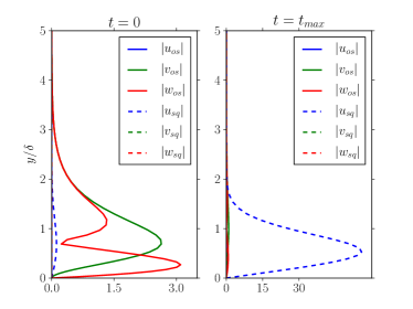
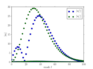
Figure 3: Optimal perturbation at $Re_{\delta}=344$ for a spanwise wave $\alpha^{*}=0$,$\beta^{*}=0.67$: a) (left) norm of the optimal perturbation with an OS-SQ decomposition; b) (right) modulus of the expansion coefficients $a_{l}^{+}$ and $a_{l}^{-}$ versus the mode number $l$ sorted by decreasing eigenvalue imaginary part.

Figure 3a shows the calculated optimal mode and its orthogonal decomposition at $t=0$ and $t=t_{max}$. As seen on this figure, the initial optimal disturbance is an OS velocity characterised by nearly spanwise vortices inside the boundary layer. Then, as expected, the perturbation transforms itself over time into Squire velocity, and at $t=t_{max}$ this perturbation is mainly a SQ velocity, that presents a large peak in the streamwise direction. This profile corresponds to the classical shape of streaks inside the boundary layer. Figure 3b shows the repartition of the modulus of the expansion coefficients $a_{l}$ in the eigenvectors basis $E^{+}$ and $E^{-}$ for this optimal perturbation:

$$\mathbf{u}_{opt}(t)=\sum_{l}a_{l}^{+}e^{-\imath\lambda_{l}t}(\mathbf{u}_{os}^{+,l}+\mathbf{u}_{sq}^{+,l})+\sum_{n}a_{n}^{-}e^{-\imath\lambda_{n}t}\mathbf{u}_{sq}^{-,n}$$

As seen in this figure, the optimal mode is a wide combination of eigenmodes $\tilde{\mathbf{u}}^{+,l}$ and $\tilde{\mathbf{u}}^{-,l}$. In the following, the mode number $l$ is sorted by decreasing eigenvalue imaginary part, such that a low mode number $l$ corresponds to an eigenvalue $\tilde{\mathbf{u}}^{l}$ with a low decay rate. We notice also the clear separation between the dominant modes associated with the coefficients $a_{l}^{+}$ and $a_{l}^{-}$, indicating that they are associated with well-separated eigenvalues. The modulus of the coefficients is large ($\gg 1$), indicating a strong non-orthogonality of the eigenvectors (for orthogonal eigenvectors we should have $|a_{l}|<1$). As the coefficients $a^{-}$ are larger than $a^{+}$ for small mode numbers $l$, they are associated with eigenmodes with smaller decay rate and the optimal mode will contain at $t=t_{max}$ essentially $\mathbf{u}_{sq}^{-,l}$ eigenvectors:

$$\mathbf{u}_{opt}(t_{max})\approx\sum_{n}a_{n}^{-}e^{-\imath\lambda_{n}t_{max}}\mathbf{u}_{sq}^{-,n}$$

IV.2 Transient growth

To characterize the link between transient growth and non-orthogonality, we define for each eigenvector $\mathbf{u}^{+,l}$ a coefficient $\Xi_{mp}^{l}$ defined as the relative norm of its OS projection:

$$\Xi_{mp}^{l}=\frac{\left\|\mathbf{u}_{os}^{+,l}\right\|_{L^{2}}}{\left\|\mathbf{u}^{+,l}\right\|_{L^{2}}}$$

This coefficient is the absolute value of the cosine of the angle between the eigenvector and the OS velocity space and thus characterises the orthogonality of the eigenvector with the set $E_{mp}^{-}$. If for all eigenvectors $\Xi_{mp}^{l}\approx 1$, then the set $E_{mp}^{+}$ is orthogonal to $E_{mp}^{-}$ and transient growth does not occur. On the other hand, transient growth is possible, with an initial perturbation equal to the OS projection of $\mathbf{u}^{+,l}$, if $\Xi_{mp}^{l}\approx 0$ for some eigenvectors $\mathbf{u}^{+,l}$ with low decay rate (i.e. associated with low mode number $l$).

The value of this coefficient $\Xi_{mp}^{l}$ and the corresponding transient growth $G_{mp}^{l}$ are plotted in Figure 4 as a function of the mode number $l$ and for various streamwise wavenumber $\alpha^{*}$. The spanwise wavenumber is $\beta^{*}=0.67$, but similar plots are obtained for $\beta$ between $1/\delta$ and $3/\delta$. As seen on this figure, for zero or low values of $\alpha^{*}$, the coefficient $\Xi_{mp}^{l}$ is very small for a large number of modes with low mode numbers $l$, that are associated with large transient growth. On the contrary for larger value of $\alpha^{*}$, the coefficient $\Xi_{mp}^{l}$ remains equal to one for low mode numbers and no transient growth is observed.

For zero streamwise wavenumber $\alpha^{*}=0$, analytical solutions can be obtained for $\mathbf{u}_{sq}^{-,l}$ and $\mathbf{u}_{os}^{+,l}$ as in Drazin and Reiddrazin04 . Outside the boundary layer, they are sinusoidal functions in the wall normal direction $y$ with a wavenumber $\mu$, independent of the Reynolds number, and solution of transcendental equations: $\mu_{l}^{+}\cot\mu_{l}^{+}=\beta\coth\beta$ and $\mu_{l}^{-}=l\pi$ for odd modes, $\mu_{l}^{+}\tan\mu_{l}^{+}=-\beta\tanh\beta$ and $\mu_{l}^{-}=(2l+1)\pi/2$ for even modes. It can be found that only the projection $\mathbf{u}_{sq}^{+,l}$ depends on the gradient of the mean flow and scales with the Reynolds number. Thus for $\alpha=0$, the coefficient $\Xi_{mp}^{l}$ scales at high Reynolds number as the inverse of the Reynolds number, indicating as expected an increase of transient growth with the Reynolds number. For low value of the streamwise wavenumber $\alpha$, the coefficient $\Xi_{mp}^{l}$ is very small for many eigenmodes with low mode number $l$, whereas for larger value of $\alpha$ the coefficient $\Xi_{mp}^{l}$ remains equal to one for small $l$ as seen in Figure 4. By looking at the shape of the eigenvectors, we conclude that the eigenmodes with very small $\Xi_{mp}^{l}$ and low mode number $l$ correspond to eigenmodes $\mathbf{\tilde{u}}^{+,l}$, having an half-wavelength $\pi/\mu$ in the normal direction $\mathbf{e}_{y}$ of the order of the boundary layer thickness $\delta$.

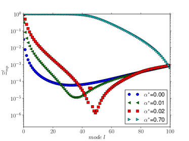
(a) $\Xi_{mp}^{l}$ for $\mathbf{u}^{+,l}$ eigenvalues

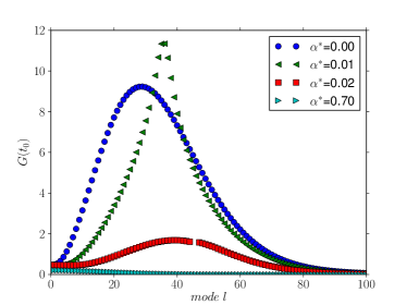
(b) transient growth $G_{mp}^{l}$ of $\mathbf{u}_{os}^{+}$

Figure 4: a) Orthogonality coefficient $\Xi_{mp}^{l}$ and b) amplification rate $G_{mp}(t_{max})$ at $t_{0}=t_{max}$ for different wavenumber $\alpha^{*}$versus the mode number $l$ sorted by decreasing eigenvalue imaginary part ($Re_{\delta}=344$, $\beta^{*}=0.67$)

V Discussion

Using the orthogonal decomposition (3) of the velocity perturbation, we have a clear demonstration of the link between transient growth and the non-orthogonality of the eigenvectors of the Orr-Sommerfeld Squire equations. Large transient growth results from the non-orthogonality of the two sets of velocity eigenmodes $E_{mp}^{+}$ and $E_{mp}^{-}$ and the ability of an OS velocity to transfer energy to a SQ velocity. To generate large transient growth, a general perturbation (as a free-stream turbulence) must induce large transfer of kinetic energy to the SQ velocity. This perturbation must thus contain OS velocity $\mathbf{u}_{os}$ associated with non-orthogonal eigenmodes $\mathbf{u}^{+,l}$ with low decay rate (i.e. such that $\Xi_{mp}^{l}\approx 0$ for small $l$). They are essentially streamwise vortex $(\alpha\ll\beta)$ with a spanwise half-wavelength and a normal half-wavelength of the order of the shear distance (the boundary layer thickness). Over time this OS velocity perturbation can develop large SQ velocity perturbation. This transient growth problem is similar to the initial value problem considered in Zaki and DurbinZaki2005 to study boundary layer transition due to free-stream turbulence. From the Squire equation they consider the initial value problem for the case of Squire modes, generated by a single Orr–Sommerfeld mode forcing. They define a coupling coefficient to characterize the ability of Orr–Sommerfeld mode to generate large Squire response. The low frequency Orr-Sommerfeld mode with large coupling coefficient are called “penetrating modes”, and they correspond to OS velocity $\mathbf{u}_{os}$ associated with non-orthogonal eigenmodes $\mathbf{u}^{+,l}$ with low decay rate. Zaki and DurbinZaki2005 attribute the large growth of disturbances generated by theses penetrating modes to exact resonance between Squire and Orr-Sommerfeld modes. Existence of resonance for a boundary layer in a semi-infinite domain is invoked by Zaki and DurbinZaki2005 , arguing that since the dispersion relation for the temporal continuous spectrum modes being identical for the Orr-Sommerfeld and Squire modes, they can have identical eigenvalues. As demonstrated in section III, this is not true in a bounded domain where exact resonance is impossible between the two sets of velocity eigenmodes $E^{+}$ and $E^{-}$. However, eigenvectors in the two sets can have close eigenvalues and thus the possibility of near resonance still exists. Thus, in bounded domains and presumably in infinite domains also, large transient growth are mainly the consequence of the non-orthogonality between the two sets $E^{+}$ and $E^{-}$ of velocity eigenmodes.

Destabilizing perturbations $\mathbf{u}_{os}$, that lead to large transient growth, are OS projection $\mathbf{u}_{os}^{+}$ of eigenvectors $\mathbf{u}^{+,l}$ with $\alpha\ll\beta$ and $\pi/\beta\approx\delta$ (i.e with $\Xi_{mp}^{l}\approx 0$ for small $l$). Their transient growth can trigger the boundary layer transition induced by free-stream turbulence. Indeed as the two sets $E^{+}$ and $E^{-}$ form a complete set, any free-stream turbulence can be expanded using these two sets. The modes in the free-stream turbulence that trigger the first instability are the destabilizing perturbations $\mathbf{u}_{os}^{+}$, that create streaks. To initiate the destabilisation of these streaks, higher frequency perturbations in the free-stream induce inflectional instability that leads to turbulent transition (Zaki and DurbinZaki2005 , Schlatter et alSchlatter2008 ).

The number of destabilizing perturbations $\mathbf{u}_{os}^{+}$ is large and a particular combination can be formed to optimize the transient growth. This is the optimal mode $\mathbf{u}_{opt}$, that combines the perturbations $\mathbf{u}_{os}^{+}$ such that $\mathbf{u}_{opt}$ is nearly zero outside the shear region because in that region the transfer term is zero. This optimal mode can model perturbations inside the boundary layer, like spanwise periodic array of small cylindrical roughness elements fixed on the wall (Fransson et alFransson2004 ).

A remarkable fact is that the shape of the transient response is nearly identical for an initial condition equal to the optimal mode $\mathbf{u}_{opt}$ and for initial conditions equal to the OS projections $\mathbf{u}_{os}^{+}$ of a large number of eigenvectors $\mathbf{u}^{+,l}$. Only the amplitude of the transient response depends on the particular initial condition. Some considerations supporting this expectation are given in Appendix A.

Appendix A. Shape of the transient response

For a wide range of initial conditions, the transient response corresponds to streaks characterised by a large peak of streamwise velocity component inside the boundary layer. The generic shape of this peak, characteristic of the transient response, can be explained by looking at the equation for the SQ streamwise velocity $u_{sq}$ obtained from the weak formulation (6) and the decomposition (3):

$$\left(\partial_{t}+\bm{\imath}\alpha U^{b}\right)u_{sq}+\frac{\beta^{2}}{k^{2}}d_{y}U^{b}v_{os}\,-Re^{-1}\mathcal{D}_{mp}^{2}u_{sq}=0$$ (13)

As large transient growth corresponds mainly to the SQ velocity $\mathbf{u}_{sq}^{-,l}$ with eigenvalues near the eigenvalue $\lambda$ of the perturbation $\mathbf{u}_{os}^{+,k}$, we are looking for solutions of (13) of the form:

$$u_{sq}=F(y)\,u_{sq}^{-,l}t\,e^{-\imath\lambda t}$$

Taking into account that $u_{sq}^{-,l}$ is an eigenvector of (13) with $v_{os}=0$, $F(y)$ is a solution of the following equation:

$$u_{sq}^{-,l}F+\frac{\beta^{2}}{k^{2}}d_{y}U^{b}v_{os}^{+,k}-Re^{-1}t\,u_{sq}^{-,k}d_{y}^{2}F=0$$

At short time, by neglecting the viscous term proportional to $Re^{-1}$, we obtain an approximate form for $F$ and thus for the transient response $u_{sq}$:

$$u_{sq}\approx-\frac{\beta^{2}}{k^{2}}v_{os}^{+,k}d_{y}U^{b}\,t\,e^{-\imath\lambda t}$$

As the mean shear $\partial_{y}U^{b}$ is zero outside the boundary layer, the streamwise transient response $u_{sq}$ is zero outside the boundary layer and depends on the normal velocity $v_{os}^{+}$ inside the boundary layer. Transient growth is obtained with perturbations $\mathbf{u}_{os}^{+,k}$ associated with small decay rates and normal wavelengths of the order of a few boundary layer thickness $\delta$. In that case $v_{os}^{+,k}\approx Cy/\delta$ in the boundary layer, and an approximation for the transient response reads:

$$u_{sq}\approx-\frac{\beta^{2}}{k^{2}}C\frac{y}{\delta}d_{y}U^{b}\,t\,e^{-\imath\lambda t}$$ (14)

In that case the shape (along $y$) $y\,d_{y}U_{b}$ of the transient response $u_{sq}$ is independent of the destabilizing perturbation $v_{os}$, and only its amplitude $\frac{\beta^{2}}{k^{2}}\frac{C}{\delta}$ is a function of the perturbation $v_{os}$ ($C$ depends on the normal wavelength of $v_{os}$).

LuchiniLuchiniJFM00 had already noted that the shape of the transient response for the optimal initial perturbation is similar to the shape for more generic initial perturbations. He pointed out that this shape looks very much like an analytical expression (due to Stewartson 1957) simply given by $y\,d_{y}U_{b}$.

References

- (1) Peter J. Schmid, “Nonmodal stability theory,” Annu. rev. Fluid Mech. 39, 129–62 (2007)
- (2) Lloyd N. Trefethen, Anne E. Trefethen, Sartish C. Reddy, and Tobin A. Driscoll, “Hydrodynamic stability without eigenvalues,” Science 261, 578–584 (1993)
- (3) P. J. Schmid and D. S. Henningson, Stability and Transition in Shear Flows. (Springer, 2001)
- (4) K. M. Butler and B. F. Farrell, “Three-dimensional optimal perturbations in viscous shear flow,” Phys. Fluids A 4, 1637–1650 (1992)
- (5) Dan S. Henningson and Satish C. Reddy, “On the role of linear mechanisms in transition to turbulence,” Phys. Fluids 6, 3, 1396–1398 (1994)
- (6) Paul Andersson, Martin Berggren, and Dan S. Henningson, “Optimal disturbances and bypass transition in boundary layers,” Phys. Fluids 11, 134–150 (1999)
- (7) P. Luchini, “Reynolds-number-independent instability of the boundary layer over a flat surface: optimal perturbations,” J. Fluid Mech. 404, 289–309 (2000)
- (8) Jens H. M. Fransson, Luca Brandt, Alessandro Talamelli, and Carlo Cossu, “Experimental and theoretical investigation of the nonmodal growth of steady streaks in a flat plate boundary layer,” Physics of Fluids 16,10, 3627–3638 (2004)
- (9) Paul Durbin and Xiaohua Wu, “Transition beneath vortical disturbances,” Annu. Rev. Fluid Mech. 39, 107–128 (2007)
- (10) Tamer A. Zaki and Paul A. Durbin, “Mode interaction and the bypass route to transition,” J. Fluid Mech. 85-111 (2005)
- (11) Lennart S. Hultgren and L. Hakan Gustavsson, “Algebraic growth of disturbances in a laminar boundary layer,” Phys. Fluids 24 (6), 1000–1004 (1981)
- (12) S. Chandrasekhar, Hydrodynamic and hydromagnetic stability (Dover Publications, 1981)
- (13) P. Holmes, J. L. Lumley, and G. Berkooz, Turbulence, Coherent Structures, Dynamical Systems, and Symmetry (Cambridge University Press, New York, 1996)
- (14) Leaf Turner, “Orthogonal, solenoidal, three-dimensional vector fields for no-slip boundary conditions,” J. Phys. A: Math. Theor. 40, 741–754 (2007)
- (15) William H. Warner, “Poloidal and toroidal potentials for solenoidal fields,” Journal of Applied Mathematics and Physics 23, 221–230 (1972)
- (16) J.R. Herring, “Approach of axisymmetric turbulence to isotropy,” Phys. Fluids 17, 859–872 (1974)
- (17) Lionel Le Penven and Marc Buffat, “A general orthogonal decomposition of solenoidal fields function of the projection of velocity and vorticity on an arbitrary direction,” J. Phys. A: Math. Gen submitted (2012)
- (18) Marc Buffat, Lionel Le Penven, and Anne Cadiou, “An efficient spectral method based on an orthogonal decomposition of the velocity for transition analysis in wall bounded flow,” Computers & Fluids 42, 62–72 (March 2011)
- (19) Alexandre Joel Chorin and Jerrold E. Marsden, A mathematical introduction to fluid mechanics (Springer, 2000)
- (20) F. Pasquarelli, A. Quarteroni, and G. Sacchi-Landriani, “Spectral approximations of the Stokes problem by divergence-free functions,” Journal of Scientific Computing 2, 1995–2026 (1987)
- (21) R. C. Di Prima and G. J. Habetler, “A completeness theorem for non-selfadjoint eigenvalue problems in hydrodynamic stability,” Archive for Rational Mechanics and Analysis 34, 218–227 (1969)
- (22) Leslie M. Mack, “A numerical study of the temporal eigenvalue spectrum of the Blasius boundary layer,” J. Fluid Mech. 73, 497–520 (1976)
- (23) Thomas M. Fischer, “A spectral Galerkin approximation of the orr-sommerfeid eigenvalue problem in a semi-infinite domain,” Numer. Math. 66, 159–179 (1993)
- (24) Robert G. Jacobs and Paul A. Durbin, “Shear sheltering and the continuous spectrum of the orr-sommerfeld equation,” Phys. Fluids 10 (8), 2006–2011 (1998)
- (25) P. G. Drazin and W. H. Reid, Hydrodynamic Stability (Cambridge University Press, 2004)
- (26) Philipp Schlatter, Luca Brandt, H. C. de Lange, and Dan S. Henningson, “On streak breakdown in bypass transition,” Physics of Fluids 20, 101205 (2008)