Exploring Torus Universes
in
Causal Dynamical Triangulations

T.G. Budd$\,{}^{a}$ and R. Loll$\,{}^{b,c}$

^a The Niels Bohr Institute, Copenhagen University
Blegdamsvej 17, DK-2100 Copenhagen Ø, Denmark.
email: budd@nbi.dk

^b Radboud University Nijmegen,
Institute for Mathematics, Astrophysics and Particle Physics,
Heyendaalseweg 135, NL-6525 AJ Nijmegen, The Netherlands.
email: r.loll@science.ru.nl

^c Perimeter Institute for Theoretical Physics,
31 Caroline St N, Waterloo, Ontario N2L 2Y5, Canada.
email: rloll@perimeterinstitute.ca

Abstract

Motivated by the search for new observables in nonperturbative quantum gravity, we consider Causal Dynamical Triangulations (CDT) in 2+1 dimensions with the spatial topology of a torus. This system is of particular interest, because one can study not only the global scale factor, but also global shape variables in the presence of arbitrary quantum fluctuations of the geometry. Our initial investigation focusses on the dynamics of the scale factor and uncovers a qualitatively new behaviour, which leads us to investigate a novel type of boundary conditions for the path integral. Comparing large-scale features of the emergent quantum geometry in numerical simulations with a classical minisuperspace formulation, we find partial agreement. By measuring the correlation matrix of volume fluctuations we succeed in reconstructing the effective action for the scale factor directly from the simulation data. Apart from setting the stage for the analysis of shape dynamics on the torus, the new set-up highlights the role of nontrivial boundaries and topology.

1   Nonperturbative quantum gravity and observables

A central quest in any approach to nonperturbative quantum gravity is for the identification and evaluation of observables: finite, invariantly defined quantities characterizing “quantum spacetime”, the Planck-scale analogue of the curved spacetime described by the classical theory of General Relativity. One reason why such observables are hard to come by is the a priori absence of a yardstick, in the form of a preferred classical “background geometry”, with respect to which distances and volumes could be measured. In a full, nonperturbative quantum formulation, such a yardstick has to be extracted from the dynamics of the quantum gravity theory, and therefore requires nontrivial knowledge of the latter. So far, only a few instances of such observables have been identified in specific candidate theories of quantum gravity. They typically depend on intrinsic properties of quantum geometry in a relational and nonlocal way. Good examples of this are various notions of “dimensionality”, obtained by relating (suitable quantum analogues of) volumes to linear distances, say, in the form of a power law, which have been used for a long time in quantum-gravitational theories obtained from dynamical triangulations [1].

The main motivation behind the work presented here is to try to push the quest for observables beyond what has been considered so far. We will do this in a specific context, that of quantum gravity constructed from Causal Dynamical Triangulations (CDT). The CDT approach has made significant progress towards a nonperturbative realization of the path integral over higher-dimensional geometries in recent years, see [2] for a comprehensive review. There is strong evidence that at large distance scales it describes a quantum universe fluctuating around an emergent classical background geometry. Its large-distance scaling properties, captured by the dynamically extracted Hausdorff [3, 4] and spectral [5] dimensions, are compatible with those of a four-dimensional spacetime. Because of the nonperturbative character of the quantum dynamics, there is no a priori guarantee that any emergent quantum spacetime will have dimension four macroscopically. Checking that this happens is therefore an important part of verifying that a quantum gravity theory possesses a good classical limit.

In addition, by examining the expectation value of the spatial volume as a function of proper time, the spacetime emergent from CDT quantum gravity has been matched with excellent accuracy to a de Sitter universe, including quantum fluctuations of the volume around it [6]. This “volume profile” is another example of the type of geometric observable we are after. It is a quantity that can be accessed relatively easily by numerical measurements, and at the same time has a transparent semi-classical geometric interpretation. From the point of view of General Relativity, it is simply the “scale factor” or “Friedmann mode” of the classical metric field $g_{\mu\nu}(x)$. In cosmological approximations to the Einstein equations, where space is described as homogeneous and isotropic, the geometry of spacetime is by assumption reduced to the dynamics of this global scale factor. In the context of full quantum gravity, the quantum dynamics of this mode and its possible implications for cosmology are clearly important to investigate, but they describe only one, global aspect of quantum spacetime. Can we go beyond the Friedmann mode in understanding the structure of quantum geometry, and how?

A natural next step is to consider modes of the geometry which are still global, but describe shape rather than scale. We will begin our exploration of this issue in spacetime dimension three. There are a number of good reasons for doing so. Firstly, as far as large-scale geometric properties are concerned, CDT quantum gravity in 2+1 dimensions appears to resemble CDT quantum gravity in 3+1 dimensions; in fact, the analysis of matching the volume profile of the emergent quantum geometry with that of a de Sitter universe was first made in the former [7]. Secondly, we have a neat and explicit way of isolating the conformal (“shape”) degrees of freedom of the two-dimensional triangulated surfaces representing space in 2+1 dimensions, at least when the spatial slices have torus topology [8, 9]. By contrast, it does not appear straightforward to isolate observables which are sensitive to global shape in the full, four-dimensional quantum theory. Thirdly, the computational effort needed in the three-dimensional setting is significantly reduced compared to that in four dimensions.

Caution is obviously advised when generalizing any results from three to four dimensions, since the local dynamics and degrees of freedom of the two quantum gravity theories are expected to be very different. In part, this is already reflected in their different phase structure (as statistical mechanical systems), which in four dimensions is much richer and has recently been shown to contain a second-order phase transition [10], something not seen in three dimensions [7]. On the other hand, in evaluating the path integral of three-dimensional quantum gravity we will not make use of the possibility to reduce the dynamical (field) degrees of freedom to a finite number of physical variables before the quantization, an essential step taken in most other treatments of quantum gravity in three dimensions [11]. In this sense, our kinematical formulation of the quantum theory resembles maximally that of four dimensions, including potential nonperturbative “entropic” effects coming from the path integral measure, which have been shown to contribute to the effective quantum dynamics in four dimensions [12].

As we shall see below, our main aim – to analyze the behaviour of shape observables in nonperturbative quantum gravity – raises some interesting and qualitatively new issues on the way, which have to do with the role of boundary conditions and global topology. These are brought to the fore by a comparison of the dynamics of torus universes with previous results in the CDT formulation, which have almost all been derived for spherical spatial topology.

This paper will analyze the quantum dynamics of volume in the new toroidal set-up, discussing in particular the issue of nontrivial boundary conditions. The complementary description of the quantum dynamics of shape for the torus universes and their interaction with the volume observable will be given in a companion paper [9].

In the next section, we recall the most important elements of Causal Dynamical Triangulations in three spacetime dimensions, and briefly review existing work on the subject. Sec. 3 specializes to the case of toroidal spatial topology and introduces the issue of boundary conditions and their relation to the volume profile. In Sec. 4 we set the stage for a comparison with classical gravity, in the form of a minisuperspace approximation depending only on the global scale factor and two global shape variables (or “moduli”). Sec. 5 discusses the measurements of volume profiles, extracted from Monte Carlo simulations, and examines how they compare with the predictions of a generalized set of classical equations of motion. In Sec. 6 we reconstruct part of the effective action that governs the quantum dynamics of the scale factor, by measuring the correlation matrix of volume fluctuations at different times. Finally, a summary and conclusions are presented in Sec. 7.

2   Causal dynamical triangulations in 2+1 dimensions

Quantizing gravity in 2+1 dimensions is a popular toy model for the full, physical theory in 3+1 dimensions. The formulation of both theories in terms of the spacetime metric $g_{\mu\nu}(x)$ looks almost identical classically, but with the drastic simplification that there are no propagating physical degrees of freedom in $d=$2+1. Unlike what is usually done in so-called “reduced phase space quantizations” [11], we will make only limited use of the simplifying properties of gravity in three dimensions when setting up the quantization. The concrete quantum-gravitational framework we will use, that of CDT, has the advantage of coming with a set of computational tools that allows us to access the nonperturbative sector of the model and evaluate interesting observables numerically, with the help of Monte Carlo simulations. As mentioned earlier, our primary goal is to learn about observables in nonperturbative quantum gravity, but we expect our investigation to lead at the same time to a better understanding of some specific features of the CDT approach.

The logic we will be following is to define the quantum theory through a continuum limit of a regularized version of the gravitational path integral, without putting in any preferred “background geometry” and without assuming that quantum fluctuations of geometry are necessarily small. Since in the present work both our simulations and the classical structures we will use for comparison lie in the Euclidean sector of the theory, we will conduct the entire discussion in Euclidean (=Riemannian) metric signature (+++). While doing this, one should keep in mind that the ensemble of geometries summed over in the Euclideanized CDT path integral is motivated by considerations inherent to the Lorentzian, causal version of the theory before the Wick rotation, as has been discussed at length elsewhere [14, 2].

Starting point is the formal continuum path integral on a three-dimensional manifold of product topology $[0,1]\times\Sigma$, with initial and final spatial geometries on $\Sigma$ labelled by $g_{ab}$ and $g^{\prime}_{ab}$,

$$Z[g_{ab},g^{\prime}_{ab}]=\int\frac{\mathcal{D}g}{\mathrm{Diff}}\exp(-S_{EH}[g]),$$ (1)

where the action is the Euclidean Einstein-Hilbert action

$$S_{EH}[g_{\mu\nu}]=-\kappa\int\mathrm{d}^{3}x\sqrt{g}(R-2\Lambda).$$ (2)

The integral in (1) is over three-dimensional geometries, redundantly parametrized by metrics $g_{\mu\nu}$, which reduce to $g_{ab}$ and $g^{\prime}_{ab}$ when restricted to the initial and final boundaries. Our notation is meant to indicate that the action of the diffeomorphism group $\mathrm{Diff}$, leading to this redundancy, must be factored out to remove infinite contributions and make sure that only physical configurations are counted.

Causal dynamical triangulations (CDT) is a particular regularization of this path integral which turns the infinite-dimensional integral into a discrete sum. This is achieved by restricting the statistical ensemble underlying (1) to piecewise linear geometries of a specific form, where each geometry consists of a “stack” of $T$ thick slices. Each slice corresponds to a minimal time step and is assembled from three-dimensional simplices, solid tetrahedra whose interior geometry is flat. Every path integral configuration therefore comes with a natural discrete time coordinate $t\in\{0,1,2,\dots,T\}$, counting the number of thick slices. By construction, the spatial geometries at fixed integer $t$ are of the form of two-dimensional triangulations $\mathbf{T}_{t}$ built from flat equilateral triangles. This includes the two boundary geometries $g_{ab}$ and $g_{ab}^{\prime}$, which are represented by $\mathbf{T}_{0}$ and $\mathbf{T}_{T}$.

The spacetime between each pair of adjacent spatial triangulations $\mathbf{T}_{t}$ and $\mathbf{T}_{t+1}$ is filled in with tetrahedra, in such a way as to make the three-dimensional geometry into a simplicial manifold. In the standard CDT formulation, we allow three types of tetrahedra, called 31-, 22- and 13-simplices, according to the distribution of their vertices on consecutive spatial slices (see Fig. 1). All tetrahedra of a particular type are geometrically identical, which is implemented in CDT by making two choices, one for the length of all timelike edges (those connecting consecutive integer-$t$ slices), and one for the length of all spacelike edges, those contained entirely in the spatial triangulations.

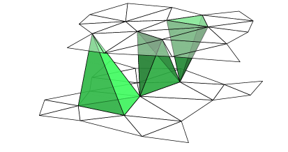
Figure 1: The three different simplex types used in CDT in 2+1 dimensions: a 31-, a 22- and a 13-simplex, labelled according to the numbers of vertices they share with the lower and upper spatial slice of integer $t$.

One consequence of using identical building blocks is that the geometry can be described essentially in combinatorial terms: to specify a triangulation one only needs to keep track of a finite list of numbers describing the neighbourhood relations among the simplices, for example, in the form of an adjacency matrix. This way the ensemble of geometries in the path integral (1) becomes a discrete set $\mathcal{T}$ of three-dimensional triangulations $\mathbf{T}$. The corresponding partition function for CDT is given by

$$Z_{\mathrm{CDT}}[\mathbf{T}_{0},\mathbf{T}_{T},T]=\sum_{\mathbf{T}\in\mathcal{T}}\frac{1}{C_{\mathbf{T}}}e^{-S_{\mathrm{CDT}}[\mathbf{T}]},$$ (3)

where $C_{\mathbf{T}}$ is the order of the automorphism group of the triangulation $\mathbf{T}$ and $S_{\mathrm{CDT}}$ is the Euclidean Einstein-Hilbert action evaluated on a piecewise linear manifold, now expressed as a function of the combinatorial properties of $\mathbf{T}$. One finds [13, 7] that the action depends on the numbers $N_{0}$ of vertices and $N_{3}$ of tetrahedra contained in $\mathbf{T}$ according to

$$S_{\mathrm{CDT}}[\mathbf{T}]=k_{3}N_{3}[\mathbf{T}]-k_{0}N_{0}[\mathbf{T}].$$ (4)

The couplings $k_{0}$ and $k_{3}$ can be expressed in terms of the bare Newton and cosmological constants as well as the space- and timelike edge lengths, but their precise form is of little interest here. The important point is that the Einstein-Hilbert action yields a function linear in the numbers $N_{d}$ of simplices of dimension $d\leq 3$. $S_{\mathrm{CDT}}$ is the most general such expression, because of identities expressing the numbers $N_{2}$ of triangles and $N_{1}$ of edges in terms of $N_{0}$ and $N_{3}$. The same is true for the numbers of 31-, 22- and 13-simplices. It also implies that the choice of spacelike and timelike edge lengths does not affect the CDT partition function other than by rescaling the bare Newton and/or cosmological constant. One can view the preferred time foliation in CDT as a discrete analogue of a proper-time (or rather proper-distance) foliation of a Riemannian manifold. Defining the edge distance between two vertices as the minimal number of edges connecting them, any vertex in the spatial triangulation $\mathbf{T}_{t}$ has a fixed edge distance $t$ to the initial boundary. In particular, both boundaries are separated by a fixed distance $T$ in lattice units, as illustrated by Fig. 2. The discrete parameter $t$ provides a convenient label that can be used in the construction of some observables, like the volume-volume correlators considered in Sec. 6 below. Whether or not it assumes the role of a physically distinguished notion of time in the continuum limit of the theory is not clear a priori. The above-mentioned matching of CDT volume profiles to continuum de Sitter universes certainly suggests that an appropriately rescaled version of $t$ can be identified with proper time on large scales and “on average” in this limit. Below in Sec. 5 we will try to match some of our results to a specific classical continuum description with a distinguished proper time.

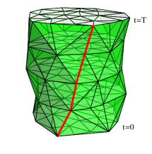
Figure 2: If one uses “edge distance” as a distance measure on causal dynamical triangulations, any vertex on the final boundary of a CDT geometry has distance $T$ to the initial boundary.

The partition function $Z_{\mathrm{CDT}}$ can be used to define the expectation value of an observable $\mathcal{O}:\mathcal{T}\to\mathbb{R}$ according to

$$\langle\mathcal{O}\rangle=\frac{1}{Z_{\mathrm{CDT}}}\sum_{\mathbf{T}}\frac{\mathcal{O}(\mathbf{T})}{C_{\mathbf{T}}}e^{-k_{3}N_{3}+k_{0}N_{0}}.$$ (5)

In Monte Carlo simulations of CDT we can measure these expectation values for certain observables. Note that the transition amplitudes $Z[\mathbf{T}_{0},\mathbf{T}_{T}]$ as function of the boundary geometries are in general not the most straightforward objects to study and interpret. This has to do with our incomplete knowledge of the Hilbert space underlying the continuum theory, and how states labelled by discrete data $\mathbf{T}$ relate to continuum wave functions “$\Psi(g_{ab})$” depending on metric data. In a nonperturbative setting like the one we are considering, “typical” states will have little resemblance with semiclassical objects, certainly not on short scales, in the same way as “typical” path integral histories do not resemble classical spacetimes. Using specific boundary geometries $\mathbf{T}_{0}$ and $\mathbf{T}_{T}$ constructed by hand runs the risk of introducing a bias in the simulations which we currently have no control over. One standard way of dealing with this issue is to avoid boundaries altogether by making time periodic, such that the topology of the triangulation becomes $S^{1}\times\Sigma$. An alternative we will be using below is to work with a set of singular boundary conditions of “big bang” or “big crunch” type, where the spatial volume shrinks to zero. This leads to a drastic reduction in the number of variables needed to describe $\mathbf{T}_{0}$ and $\mathbf{T}_{T}$ and therefore to a situation which is much better controlled.

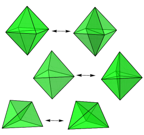
Figure 3: A set of local update moves on CDT configurations in 2+1 dimensions: flipping the diagonal of the central spatial square (top); subdividing the central spatial triangle into three (middle); substituting the central timelike triangle by its dual timelike link (bottom).

To approximate expectation values of observables using Monte Carlo simulations one needs to generate a large set of random CDT configurations according to the Boltzmann distribution in (3), which can be accomplished by a Markov process. In practice, we start by constructing by hand a triangulation $\mathbf{T}$ with the desired topology and satisfying the desired boundary conditions. We then apply a large number of random update moves on $\mathbf{T}$, where each move occurs with a probability carefully chosen to satisfy a detailed balance condition. In the case of CDT in 2+1 dimensions a suitable set of local update moves is shown in Fig. 3, see [13, 7] for more details. We should point out that the Monte Carlo code used to derive the results presented below is independent of what was used in previous published work, for example, in [7, 16, 17].

As already mentioned, properties of CDT quantum gravity in three spacetime dimensions have so far been studied only for spherical spatial slices, that is, $\Sigma=S^{2}$. The phase structure of the underlying statistical model was investigated in [7, 18]. The phase diagram is parametrized by the bare constants $k_{0}$ and $k_{3}$ introduced above. As usual in dynamically triangulated systems, the bare cosmological constant (which in our case can be identified with $k_{3}$) must be fined-tuned from above to a critical line in phase space to obtain an infinite-volume limit (divergent $N_{3}$). What remains is a one-dimensional phase space parametrized by $k_{0}$. For a range of $k_{0}$-values, the system is found to be in a phase of extended, three-dimensional geometry, with a volume profile that can be matched to that of a round three-sphere, the Euclidean de Sitter universe. As $k_{0}$ increases, one finds a (first-order) phase transition to a phase of degenerate geometry, where neighbouring spatial slices decouple, and which seems to be uninteresting from a physical point of view. An interesting feature of this system is that the quantum spacetime appears to be dynamically driven towards an $S^{3}$-topology, although all geometries in the ensemble had product topology $S^{1}\times S^{2}$ (with time compactified to a circle) to start with.

Studying a diffusion process on the CDT ensemble [16], further evidence was gathered that the emergent quantum geometry on large scales is indeed a de Sitter universe. A measurement of the spectral dimension on short scales found a value compatible with 2 [16], reminiscent of the dynamical dimensional reduction seen in CDT quantum gravity in 3+1 dimensions [5]. Deviations from sphericity of the spatial slices in the de Sitter phase of CDT have been studied in [19], using an embedding in three-dimensional flat space to set up a spherical harmonic analysis. An generalized version of CDT quantum gravity in 2+1 dimensions, including additional terms in the action motivated by Hořava-Lifshitz gravity, was investigated numerically in [20].

In terms of solving 2+1 Causal Dynamical Triangulations exactly, perhaps unsurprisingly for a three-dimensional statistical model, our knowledge is still rather incomplete. Matrix model methods have been invoked to study the combinatorics of a single thick slice ($\Delta t=1$) and extract information about the system’s phase structure, transfer matrix and behaviour under renormalization [21]. One possible strategy for solving the gravity theory analytically is to reduce the number of CDT configurations to simplify the solution of the combinatorial problem without (hopefully) changing the universality class of the continuum theory. By imposing additional order on spatial slices (more specifically, by requiring them to have a product structure as two-dimensional triangulations) and by using an arsenal of statistical mechanical tools, a Hamiltonian for the scale factor was derived analytically, for the case of cylindrical spatial slices [22]. Using an even stronger restriction of the CDT ensemble by requiring spatial slices at integer-$t$ to be flat tori, it could be shown that the combinatorics of the one-step propagator is that of a set of vicious walkers [23]. Despite the finite dimensionality of this model of “CDT quantum cosmology”, its continuum limit and full dynamics are at this stage not known. It is a precursor of our present numerical investigation in the sense of using toroidal universes and trying to extract a quantum dynamics in terms of three global parameters: the spatial volume and two moduli parameters, describing the tori’s global shape. – Three-dimensional CDT quantum gravity with toroidal slices is the subject we will turn to next.

3   Torus universes in CDT

In this section we present an initial investigation of the spatial volume profiles in CDT simulations with $\Sigma=T^{2}$, and determine which boundary conditions yield the most interesting dynamics. We will first consider periodic boundary conditions, which have been used extensively in CDT with spherical spatial topology. Note that periodic boundary conditions induce a time translation symmetry in the system: shifting the time $t\to t+1$ (modulo $T$) maps the ensemble $\mathcal{T}$ of CDT configurations to itself and leaves the action $S_{\mathrm{CDT}}$ invariant. Consequently, the ensemble average $\langle V(t)\rangle$ of the spatial volume profile is time-independent and therefore contains little information.

However, it has been observed in the spherical case, both in 2+1 [7] and 3+1 dimensions [3], that for individual spacetime configurations and sufficiently large time extent $T$ the simplices do not distribute themselves homogeneously in time, but “condense” into a subinterval in time where spatial volumes are macroscopic, while the remaining time slices are reduced to minimal spatial volume. One can therefore obtain a nontrivial profile by averaging the spatial volumes not at fixed time $t$, but at a fixed time $t^{\prime}$ relative to the location of the centre of the extended region along the time axis. The resulting volume profile is illustrated in Fig. 4 (left), which shows a typical volume distribution $V(t^{\prime})$ together with the expectation value $\langle V(t^{\prime})\rangle$. To high accuracy the expectation value $\langle V(t^{\prime})\rangle$ coincides with the spatial volume of a proper-time foliation of the three-sphere, lending credence to the conjecture that Euclidean de Sitter space emerges dynamically from CDT quantum gravity on $S^{1}\times S^{2}$.

One might therefore have expected a similar behaviour for CDT on the torus, but according to our current understanding the situation appears to be different. In none of the simulations performed, with a wide range of three-volumes $N_{3}\!\leq 250\,000$, time extents $T\!\leq\!100$, and couplings $k_{0}\!\in\![2.5,4.5]$, did we observe a breaking of the time translation symmetry or any tendency of spatial slices to degenerate to configurations of minimal volume. This is illustrated by the right-hand side of Fig. 4, which shows a typical volume profile from a CDT simulation with spatial tori and $T=70$ time slices. Of course, the absence of degenerate spatial geometries does not prove that the classical limit has time translation symmetry. A more detailed analysis, for instance, involving the distribution of Fourier modes of $V(t)$, would be necessary to make more definite statements.

At this stage, we do not know which feature of the torus topology in CDT is responsible for this quite different behaviour, compared to that for spherical topology. One way in which the CDT configurations differ is in the number of triangles in a minimal triangulation of $\Sigma$ (minimal in the sense of being compatible with the simplicial manifold character and the overall topology of spacetime, i.e. preventing the geometry from “pinching off”). For the sphere the minimal configuration is given by the boundary of a tetrahedron, which consists of four triangles. By contrast, a triangulation of the torus requires a minimum of 14 triangles and therefore substantially more tetrahedra are needed to produce a “stalk” of minimal spatial volume. This could certainly have an effect on the simulations, because the extra cost of the stalk (as measured by the $N_{3}$-term in the CDT action) may no longer be outweighed by the entropic gain of the tetrahedra clumping together. However, this is an effect one would expect to disappear for sufficiently large three-volume. Once we have understood better the effective dynamics of CDT – which is precisely part of the motivation behind the present investigation – we should be able to give a more satisfactory explanation of the global behaviour of the scale factor and its relation to topology.

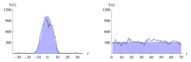
Figure 4: Comparing volume profiles of CDT with topology $S^{1}\times S^{2}$ (left) and $S^{1}\times T^{2}$ (right). The solid curves represent typical (random) configurations, while the shaded areas correspond to the expectation values $\langle V(t^{\prime})\rangle$ and $\langle V(t)\rangle$ respectively. (Sphere data taken at total volume $N_{3}\!=\!40\,000$, torus data at $N_{3}\!=\!60\,000$.)

The drawback of the apparent absence of symmetry breaking in time of the volume profiles is that it deprives us of an interesting observable. To bring about a nontrivial time dependence of the spatial volume, we will in the following trade the usual periodic boundary conditions for suitable fixed boundaries, involving degenerate boundary geometries of zero volume. For spherical topology such boundary conditions at $t=0$ and $t=T$ are not likely to have much of an effect, since the system wants to pinch off dynamically at the north and south pole of the de Sitter universe anyway. By contrast, we will see that similar boundary conditions for CDT on the torus will have an impact on the dynamics of the spatial volume, since minimal spatial volumes do not occur with periodic boundary conditions.

In addition to a nontrivial volume profile we are also interested in creating a situation where the shape parameters of the tori evolve nontrivially in time. These two requirements can be satisfied simultaneously by taking an initial torus elongated in one direction and a final torus elongated in the opposite direction. The difficulty with choosing boundary triangulations of this kind is that (i) we need many boundary triangles, and (ii) there is still considerable ambiguity in how we put them together. Fortunately there is an easier option, namely, to take the boundary to be completely degenerate in one of the two directions, resulting in the collapse of the two-dimensional torus to a one-dimensional circle, described merely in terms of the number $l_{0}$ of its edges. To illustrate the idea, Fig. 5 shows a piece of a CDT configuration with an initial boundary consisting of $l_{0}=8$ edges.

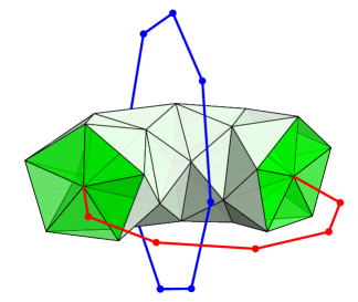
Figure 5: A degenerate initial boundary at $t\!=\!0$ consisting of $l_{0}\!=\!8$ edges (solid red curve). Moving away from $t\!=\!0$ in discrete time steps, one obtains a sequence of solid tori. The light triangles belong to the boundary of the triangulated solid torus at $t\!=\!1$. If we choose the final singularity according to the blue curve, we end up with the Hopf foliation of $S^{3}$.

With this choice, the topology of the spacetime region $0\leq t\leq t^{\prime}$ for some $0<t^{\prime}<T$ becomes that of a solid torus. If we impose similar boundary conditions on the final boundary, the same will hold for the region $t^{\prime}\leq t\leq T$. Therefore the most general spacetime topology is that of a pair of solid tori glued along their boundaries (in this case corresponding to the torus at time $t^{\prime}$). This can be done in several topologically inequivalent ways, giving rise to $S^{2}\times S^{1}$, $S^{3}$ or, more generally, a lens space $L(p,q)$ (see, for example, [24]). For our purposes the second option is the most interesting, because it is the simplest topology that allows for a nontrivial shape evolution. It is achieved by taking the initial and final singularity such that together they form the so-called Hopf link in $S^{3}$. This is illustrated in Fig. 5, where the final singularity is shown in blue and the embedding space $\mathbb{R}^{3}$ represents $S^{3}$ with one point removed (for example, after stereographic projection). The foliation of the three-sphere by tori obtained in this way is known as the Hopf foliation.

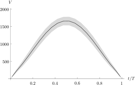
Figure 6: Volume profile for $N_{3}\!=\!60\,000$ and $T\!=\!19$, with boundaries consisting of $l_{0}\!=\!l_{1}\!=\!60$ edges and $k_{0}\!=\!2.5$. The shaded area corresponds to the standard deviation in $V(t)$ and gives an idea of the size of the quantum fluctuations. Error bars are not shown explicitly, but are of the order of $0.1\%$.

The results presented below are based on CDT simulations with time extension $T=19$. Unless indicated otherwise, we take the length $l_{1}$ of the final singularity at $t=T$ to be identical to the length $l_{0}$ of the initial singularity at $t=0$, in order to maintain time-reversal symmetry. Fig. 6 shows the expectation value $\langle V(t)\rangle$ of the spatial volume, for a simulation with a fixed number $N_{3}=60\,000$ of tetrahedra, boundary length $l_{0}=60$, and coupling $k_{0}=2.5$. We observe a clear expansion of the volume at early times and a contraction at late times, indicating a nontrivial dynamics of the spatial volume. Moreover, the expansion close to the singularity is roughly linear, which is in accordance with the initial geometry being one-dimensional. Before exploring other values of $N_{3}$, $l_{0}$, and $k_{0}$ more systematically, let us survey which classical gravitational solutions we may want to compare our results to.

4   Classical solutions with torus topology

Classical solutions of General Relativity with Euclidean signature are given by the stationary points of the Euclidean Einstein-Hilbert action (2), determined by solutions to the Einstein equations

$$R_{\mu\nu}-\frac{1}{2}R\,g_{\mu\nu}+\Lambda\,g_{\mu\nu}=0,$$ (6)

which in three dimensions are equivalent to (see, for example, [11])

$$R_{\mu\nu\rho\sigma}=\Lambda(g_{\mu\rho}g_{\nu\sigma}-g_{\mu\sigma}g_{\nu\rho}).$$ (7)

In other words, the solutions have constant scalar curvature $R$ and are therefore locally isometric to the three-sphere ($\Lambda\!>\!0$), flat Euclidean space ($\Lambda\!=\!0$) or hyperbolic space ($\Lambda\!<\!0$), depending on the sign of the cosmological constant $\Lambda$. As a consequence, classical General Relativity in three dimensions has no local degrees of freedom.

To find its solutions explicitly, we switch to the ADM formalism and rewrite the metric $g_{\mu\nu}$ in terms of the spatial metric $g_{ab}$, the shift vector $N^{a}$ and the lapse function $N$ as

$$ds^{2}=N^{2}dt^{2}+g_{ab}(dx^{a}+N^{a}dt)(dx^{b}+N^{b}dt).$$ (8)

In terms of these the Einstein-Hilbert action reads

$$S_{ADM}[g_{ab},N^{a},N]=-\kappa\int\mathrm{d}t\int\mathrm{d}^{2}x\sqrt{{}^{(2)}\!g}\,N\left(K^{2}-K_{ab}K^{ab}+{}^{(2)}\!R-2\Lambda\right),$$ (9)

where ${}^{(2)}\!g$ is the determinant of the spatial metric, ${}^{(2)}\!R$ the two-dimensional scalar curvature and $K_{ab}$ the extrinsic curvature tensor

$$K_{ab}=\frac{1}{2N}\left(\dot{g}_{ab}-\nabla_{a}N_{b}-\nabla_{b}N_{a}\right).$$ (10)

The only difference with the usual Lorentzian signature case is a plus instead of a minus sign in front of the potential term $({}^{(2)}\!R-2\Lambda)$ in the action, relative to the kinetic term $(K^{2}-K_{ab}K^{ab})$, which remains unchanged. If one puts the lapse $N$ to 1, the set of constant-$t$ surfaces defines a proper-time foliation of the spacetime manifold. To make the gauge choice $N\!=\!1$ therefore seems particularly suggestive when comparing to CDT.

One can find the classical solutions by putting (9) into canonical form (see [25] or [11]) and imposing the constant mean curvature (CMC) gauge condition in which one can solve the dynamics completely. In this gauge the classical solutions for the torus can be shown to be spatially flat. The lapse only depends on time, while the shift can be chosen to vanish, which means that on shell the foliation fixed by the CMC gauge is a proper-time foliation, up to a rescaling of the time variable.

It follows that in general all solutions can be obtained from a minisuperspace model, where spatial homogeneity is imposed from the outset. To achieve this, let us set $N\!=\!N(t)$, $N^{a}\!=\!0$ and $g_{ab}(t)\!=\!V(t)\hat{g}_{ab}(\tau_{i}(t))$, where $\hat{g}_{ab}(\tau_{i})$ denotes the flat unit-volume metric on the torus parametrized by the two real moduli $\tau_{1}$ and $\tau_{2}$,

$$\hat{g}_{ab}(\tau)=\frac{1}{\tau_{2}}\begin{pmatrix}1&\tau_{1}\\ \tau_{1}&\tau_{1}^{2}+\tau_{2}^{2}\end{pmatrix}.$$ (11)

Substituting this ansatz into (9) we obtain the minisuperspace action

$$S[V,\tau_{i},N]=\kappa\int\mathrm{d}t\left(\frac{1}{2N}\left(-\frac{\dot{V}^{2}}{V}+V\frac{\dot{\tau}_{1}^{2}+\dot{\tau}_{2}^{2}}{\tau_{2}^{2}}\right)+2N\Lambda V\right).$$ (12)

As desired, this is now a function of global scale (the two-volume $V$) and global shape (in the form of the $\tau_{i}$). Note that there is no contribution coming from the Ricci scalar ${}^{(2)}\!R$, because its integral over the torus vanishes by virtue of the Gauss-Bonnet theorem. To find the classical solutions, we identify two conserved quantities $\cal E$ and $p$, given by

$${\cal E} =\frac{1}{2N}\left(-\frac{\dot{V}^{2}}{V}+V\frac{\dot{\tau}_{1}^{2}+\dot{\tau}_{2}^{2}}{\tau_{2}^{2}}\right)-2N\Lambda V,$$ (13)

$$p =\frac{V}{N}\frac{\sqrt{\dot{\tau}_{1}^{2}+\dot{\tau}_{2}^{2}}}{\tau_{2}}.$$ (14)

Moreover, variation with respect to the lapse $N(t)$ yields the initial value condition ${\cal E}\!=\!0$. Imposing the proper-time gauge $N\!=\!1$, one easily finds the most general solution for the spatial volume $V(t)$ up to time translation and time reversal,

$$V(t)=\begin{cases}\frac{p}{2\sqrt{\Lambda}}\sin(2\sqrt{\Lambda}\,t)&\text{if }\Lambda>0\\ p\,t&\text{if }\Lambda=0\hskip 56.9055pt({\cal E}\!=\!0)\\ \frac{p}{2\sqrt{-\Lambda}}\sinh\left(2\sqrt{-\Lambda}\,t\right)&\text{if }\Lambda<0.\end{cases}$$ (15)

In addition, we have the static solution $\dot{V}\!=\!p\!=\!0$ for $\Lambda\!=\!0$ and exponentially expanding/contracting solutions $V(t)\!=\!\exp\left(\pm 2\sqrt{-\Lambda}t\right)$ and $p\!=\!0$ for $\Lambda\!<\!0$.

From (15), the only solution with both an initial and a final singularity, at $t\!=\!0$ and $t\!=\!T\!=\!\pi/(2\sqrt{\Lambda})$ respectively, is obtained when $\Lambda\!>\!0$. The corresponding general solution for the modular parameter $\tau\!=\!\tau_{1}+i\tau_{2}$ traces out a geodesic in the Poincaré upper half-plane (the Teichmüller space of a genus-1 surface), whose speed is determined by $p$ in (14). Reaching a big bang or big crunch singularity of the spacetime corresponds to $\tau$ hitting the boundary of Teichmüller space, which is associated with degenerate tori. The boundary conditions $\tau(0)\!=\!0$ and $\tau(T)\!=\!i\infty$ give precisely the Hopf foliation of the three-sphere, described in Sec. 3 above. The general solution with these boundary conditions is parametrized by the lengths $l_{0}$ and $l_{1}$ of the singularities and is given by the spacetime metric

$$ds^{2}=dt^{2}+l_{0}^{2}\cos^{2}(\sqrt{\Lambda}\,t)\,dx^{2}+l_{1}^{2}\sin^{2}(\sqrt{\Lambda}\,t)\,dy^{2}.$$ (16)

The three-volume $V_{3}$ of this geometry is $V_{3}\!=\!l_{0}l_{1}/(2\sqrt{\Lambda})$, which directly relates the cosmological constant $\Lambda$ and the total volume $V_{3}$. One also finds $p\!=\!l_{0}l_{1}\sqrt{\Lambda}$. However, when trying to compare the corresponding volume profile

$$V(t)=\frac{l_{0}l_{1}}{2}\sin(2\sqrt{\Lambda}\,t)$$ (17)

directly to measurements in CDT simulations, one runs into a difficulty. The total time extension $T\!=\!\pi/(2\sqrt{\Lambda})$ of the classical solution (17) is fixed in terms of $\Lambda$ (equivalently, in terms of the three-volume and the boundary conditions), whereas in the CDT simulations $T$ appears a priori as an additional, free parameter set by hand.

This is a specific case of a more general issue, namely, under what circumstances particular CDT set-ups and their associated observables can be meaningfully compared to aspects of the classical theory of General Relativity, and vice versa. To start with, there is of course no guarantee that an arbitrary classical solution can be obtained from a nonperturbative path integral, with suitable boundary conditions. Returning to the problem at hand, one way of trying to address the mismatch between the parameters of the classical torus solutions and those of the CDT model with specific boundary conditions imposed is to generalize the classical solutions one is comparing to. The idea is to gauge-fix the lapse in the minisuperspace action (12) before varying the action, without adding the (then missing) Hamiltonian constraint by hand afterwards. As we will see, one gains a free parameter by doing this, and can write down a set of classical solutions which satisfy the desired boundary conditions. In the next section we will examine how well these generalized solutions fit the measured simulation data.

Whether or not such an ansatz captures the nonperturbative dynamics of the 2+1 CDT model with nontrivial boundaries correctly is difficult to argue on general grounds, because of our lack of explicit control over the details of the former. Apart from the already mentioned influence of boundary conditions and global topology, this includes the question to what extent the discrete “edge distance” $t$ on CDT configurations described in Sec. 2 in a particular continuum limit can be related to any continuum notion of a local (proper) time, which one can identify on a classical ensemble of spacetime metrics, through gauge-fixing or otherwise. Although the de Sitter results are strong evidence that such an identification works on large scales for the global volume variable, this does not imply that these two notions of time can be identified at a local, microscopic level.

Keeping these comments in mind, we will now construct an ensemble of smooth classical metrics in proper-time gauge, each of whose members has an initial and a final boundary at exact proper-time distance $T$, together with a set of generalized equations for the global scale and shape variables. In line with our previous discussion, our starting point will be the Einstein-Hilbert action in ADM form, with the lapse fixed to $N\!=\!1$, yielding

$$S[g_{ab},N^{a}]=-\kappa\int_{0}^{T}\mathrm{d}t\int\mathrm{d}x\sqrt{g}\left(K^{2}-K_{ab}K^{ab}+R-2\Lambda\right).$$ (18)

This means that

$$\left.\frac{\delta S}{\delta N}\right|_{N=1}=-\sqrt{g}(K_{ab}K^{ab}-K^{2}+R-2\Lambda)$$ (19)

is no longer required to vanish, although its constancy in time is still guaranteed by the other equations of motion. Note that the functional form of the right-hand side of (19) is exactly that of the Hamiltonian constraint (in Euclidean signature), whose vanishing is normally used to solve for the trace part of the spatial metric in terms of the traceless degrees of freedom.

Let us determine which effect this has on the family of homogeneous solutions for the torus universe. We still have the conserved quantities $\cal E$ and $p$ from (13) and (14), with $N$ set to 1. However, $\cal E$ is no longer required to vanish and serves as an additional parameter in the family of solutions, which we can tune to arrive at a desired total time extent $T$. Restricting to the solutions with two singularities and non-vanishing $p$, we find a family of volume profiles,

$$V(t)=\begin{cases}l_{0}l_{1}\frac{\sinh\left(\sqrt{-\Lambda}(T-t)\right)\sinh\left(\sqrt{-\Lambda}\,t\right)}{\sinh^{2}\left(\sqrt{-\Lambda}\,T\right)}&\text{if }\Lambda<0\\ l_{0}l_{1}(T-t)t/T^{2}&\text{if }\Lambda=0\hskip 71.13188pt({\cal E}\!\not=\!0)\\ l_{0}l_{1}\frac{\sin\left(\sqrt{\Lambda}(T-t)\right)\sin\left(\sqrt{\Lambda}\,t\right)}{\sin^{2}\left(\sqrt{\Lambda}\,T\right)}&\text{if }0<\Lambda<\left(\frac{\pi}{T}\right)^{2}.\end{cases}$$ (20)

The underlying line element, say, for the case of positive $\Lambda$, generalizes (16) to the four-parameter family

$$ds^{2}=dt^{2}+l_{0}^{2}\,\frac{\sin^{2}(\sqrt{\Lambda}\,(T-t))}{\sin^{2}(\sqrt{\Lambda}\,T)}\,dx^{2}+l_{1}^{2}\,\frac{\sin^{2}(\sqrt{\Lambda}\,t)}{\sin^{2}(\sqrt{\Lambda}\,T)}\,dy^{2}.$$ (21)

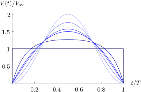
Figure 7: The spatial volume $V(t)$ of (20) of the classical solutions, normalized by its time average $V_{\mathrm{av}}\!=\!V_{3}/T$, for different values of $v\!=\!V_{3}/(l_{0}l_{1}T)$. The value of $v$ increases monotonically from 0 to $\infty$ as $\Lambda$ ranges between $-\infty$ and $(\pi/T)^{2}$ (for fixed $l_{0}$, $l_{1}$ and $T$). The curves, from dark to light, correspond to $v\!=\!0$ (flat), $v\!=\!0.01$, $v\!=\!1/6$ (parabola, $\Lambda\!=\!0$), $v\!=\!1/\pi$ (sine, $\Lambda\!=\!(\pi/2T)^{2}$), $v\!=\!2$, and $v\!=\!\infty$ (sine squared, $\Lambda\!=\!(\pi/T)^{2}$).

The two associated constants of motion can be expressed as functions of the four parameters $(l_{0},l_{1},\Lambda,T)$ according to

$${\cal E}=2\Lambda l_{0}l_{1}\,\frac{\cos(\sqrt{\Lambda}T)}{\sin^{2}(\sqrt{\Lambda}T)},\;\;\;p=\frac{l_{0}l_{1}\sqrt{\Lambda}}{\sin(\sqrt{\Lambda}T)}.\;\;\;\;\;\;\;\;\;\;\left(0<\Lambda<(\pi/T)^{2}\right)$$ (22)

For fixed $l_{0}$, $l_{1}$, and $T$, the three-volume computed from (20) increases monotonically as a function of $\Lambda$ from $V_{3}\!=\!0$ at $\Lambda\!=\!-\infty$ to $V_{3}\!=\!\infty$ at $\Lambda\!=\!(\pi/T)^{2}$. In Fig. 7 we have plotted the analytic volume profiles normalized by their time average $V_{\mathrm{av}}\!=\!V_{3}/T$ for various values of $\Lambda$. The shape of the profile only depends on the dimensionless quantity $v\!=\!V_{3}/(l_{0}l_{1}T)$. For $v\!\to\!0$ we find a flat profile, for $v\!=\!1/6$ a parabola, for $v\!=\!1/\pi$ a sine, and for $v\!\to\!\infty$ a sine-squared profile. Note also that the minisuperspace action (for $N\!=\!1$), when evaluated on solutions, is positive, despite the negative kinetic term for the volume in (12). Like the three-volume, the action is monotonically increasing as a function of $\Lambda$ (with everything else held fixed), from $S\!=\!0$ at $\Lambda\!=\!-\infty$ to $S\!=\!+\infty$ for $\Lambda\!=\!(\pi/T)^{2}$.

5   Measurement of volume profiles

Having derived the volume profiles (20) for the generalized equations of motion, we will now return to the data from the Monte Carlo simulations, to see whether they can be fitted to the new, wider range of shapes. In the current set-up, the CDT partition function depends on four free parameters (five if we counted the boundary lengths $l_{0}$ and $l_{1}$ separately): the time extension $T$, the discrete three-volume $N_{3}$, the coupling $k_{0}$, and the boundary length $l_{0}$. Because probing the full parameter space would be very time-consuming, we fix the three-volume to $N_{3}=60\,000$ and the total time to $T=19$, and perform simulations for a wide range of values of the coupling $k_{0}$ and the boundary length $l_{0}$.

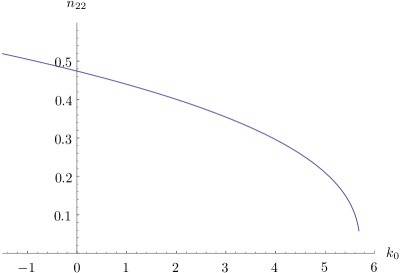
Figure 8: The measured fraction $n_{22}$ of simplices of type $22$ as function of the coupling constant $k_{0}$.

To determine the relevant range of the coupling $k_{0}$, recall from Sec. 2 that $k_{0}$ – which can essentially be identified with the bare inverse Newton constant – is the free, tunable phase space parameter that remains after fine-tuning the bare cosmological constant. Of course, we expect the phase diagram of 2+1 CDT quantum gravity on the torus to have the same qualitative features as on the sphere, with an extended quantum spacetime only found below some value $k_{0}^{\ast}$. Like in the spherical case [7], the effect of increasing $k_{0}$ is to reduce the number $N_{22}$ of 22-simplices in favour of 31- and 13-simplices. As illustrated by Fig. 8, the fraction $n_{22}:=N_{22}/N_{3}$ of simplices of type 22 in our simulation collapses to (nearly) zero when $k_{0}$ approaches the critical value $k_{0}^{\ast}\approx 5.6$. Since the 22-simplices provide the coupling between consecutive spatial triangulations, the spatial geometries in the region $k_{0}>k_{0}^{\ast}$ of phase space effectively decouple, and spacetime loses any classical physical interpretation. Since we are interested in a theory which possesses a good classical limit, and therefore is macroscopically extended in both time and space, we will from now on restrict our attention to the “physical” phase $k_{0}<k_{0}^{\ast}$, and also make sure to not get too close to the phase transition $k_{0}^{\ast}$, where the fluctuations in the spatial volume are large.

The expectation value $\langle V(t)\rangle$ presented earlier in Fig. 6 turns out to be well described by the volume profile for $v\!=\!0.98$ (c.f. Fig. 7). More systematically, Fig. 9a shows our results for fixed $l_{0}\!=\!60$ and $k_{0}$ varying from $1.0$ to $5.0$ in steps of $0.5$. Clearly, as we increase $k_{0}$ towards the phase transition, the shape of the volume profile becomes flatter, which corresponds to the parameter $v$ approaching zero. This is in line with the discussion above, in the sense that a complete decoupling of the spatial triangulations would lead to a flat volume profile with $v\!=\!0$.

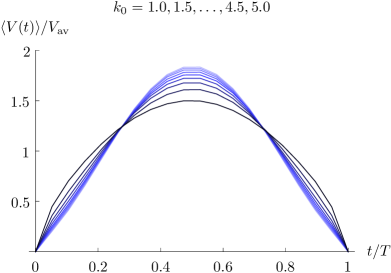
(a)

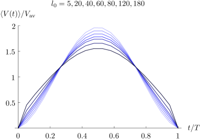
(b)

Figure 9: Normalized volume profiles for several simulations with $N_{3}\!=\!60\,000$: (a) at fixed $l_{0}\!=\!60$, for various values of $k_{0}$, and (b) at fixed $k_{0}\!=\!2.5$, for various boundary lengths $l_{0}$. The lightest curves correspond to $k_{0}\!=\!1.0$ and $l_{0}\!=\!5$ respectively.

Conversely, to obtain the curves in Fig. 9b, we fixed $k_{0}\!=\!2.5$ but varied the boundary length $l_{0}$ to take the values 5, 20, 40, 60, 80, 120, and 180. As $l_{0}$ decreases, we observe an approach towards the sine-squared shape, i.e. $v\to\infty$, in accordance with the dependence of $v$ on the boundary lengths in the analytic continuum formulation.

If we were sufficiently confident that the system was well approximated by the classical minisuperspace description, we could at this stage test the classical relation $v\!=\!V_{3}/(Tl_{0}^{2})$ quantitatively. However, we should probably not put too much trust in this classical description. To start with, it is unclear how significant the qualitative similarity between the measurements and the classical solutions really is; it could be due to the rather generic nature of the classical volume profiles, which represent roughly the smoothest profiles with a given slope and time-reversal symmetry. More significant tests of the conjectured classical limit would involve studying higher-order corrections to the volume profile.

The situation is different when we consider CDT set-ups which are not symmetric under time reversal, by using unequal boundary lengths $l_{0}$ and $l_{1}$ in the simulations. In this case, the classical solutions (20) yield a nontrivial prediction, namely, that the volume profile remain symmetric. To test this prediction, we have performed simulations with fixed initial singularity length $l_{0}\!=\!60$ and varying final singularity length $l_{1}\!=\!5$, 20, 40, 60, 80 and 120. The results are shown in Fig. 10, from which it is clear that the expected symmetry is not present in our system when $l_{0}\!\neq\!l_{1}$. Instead of identical slopes at the two boundaries, we see that the slope at the initial boundary hardly changes when changing $l_{1}$. If the classical solutions we are comparing to are the correct ones, this could mean that the information about the geometry at $t\!=\!T$ is not propagated all the way to small $t$, in the sense that spatial geometries at small time $t$ are oblivious to the final boundary conditions. In classical gravity, however, the geometry is sensitive to the boundary conditions no matter how far one is from the boundary.

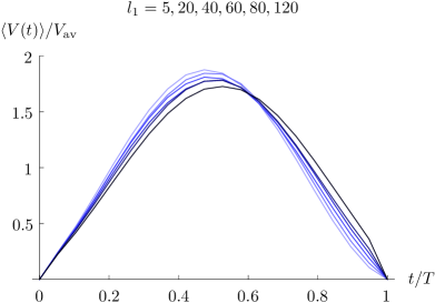
Figure 10: Normalized volume profiles for $k_{0}\!=\!2.5$, $N_{3}\!=\!60\,000$ and $T\!=\!19$. The initial singularity has fixed length $l_{0}\!=\!60$, while the final singularity length is varied with $l_{1}\!=\!5,20,40,60,80,120$ ($l_{1}\!=\!120$ corresponds to the darkest curve).

There are potentially a number of reasons which could explain discrepancies between the data and the classical solutions (20): (a) at least for certain boundary conditions, the classical limit of CDT could be genuinely different from the generalized minisuperspace ansatz we obtained from general relativity, (b) our systems could be too far from classicality or too small to make a sensible comparison, (c) we could be making the wrong identification of discrete and continuum boundary conditions; for example, the path determined by the singularity could exhibit a random walk behaviour in the three-dimensional triangulation, leading to an anomalous scaling of the continuum singularity length with the discrete $l_{0}$ (which should be taken into account when investigating a dependence on boundary lengths, say).

At the system sizes we have been considering probably not much will be learned by making more detailed measurements of the volume profiles, since it is difficult to distinguish alternatives for the classical dynamics from quantum corrections. As a potentially more fruitful strategy, we will from now on assume that for the range of system sizes we are considering, there exist effective actions which describe the CDT systems, and will try to “reconstruct” these effective actions or at least deduce some of their properties directly from the data. Once we manage to significantly narrow down the relevant terms in a given effective action, we will in principle be able to study their scaling properties when approaching the continuum limit. In the next section, we will reconstruct the kinetic term for the two-volume from measuring a particular correlation function. Forthcoming work will analyze the contribution from the moduli parameters to the effective action [9].

6   Effective action from volume correlations

Suppose that the Euclidean effective action $S[V]$ for the spatial volume in 2+1 dimensional CDT is local in time and can be written as the integral of a Lagrangian $\mathcal{L}(V,\dot{V})$ according to

$$S[V]=\int_{0}^{T}\mathrm{d}t\,\mathcal{L}(V,\dot{V}).$$ (23)

Assuming time reversal symmetry leads to the condition $\mathcal{L}(V,-\dot{V})=\mathcal{L}(V,\dot{V})$, which implies that only even powers of $\dot{V}$ can appear in the Lagrangian. Given a proper set of boundary conditions, the action $S[V]$ will have a unique classical solution $V_{0}(t)$, satisfying $\delta S[V_{0}]\!=\!0$, which should describe the expectation values $\langle V(t)\rangle$ of the volume profile measured in the simulations, at least for sufficiently large $V(t)$ that are unaffected by quantum corrections.

Since in general $V_{0}(t)$ depends on all terms in the Lagrangian $\mathcal{L}$, it is difficult to deduce specific information about the form of $\mathcal{L}$ from measurements of $\langle V(t)\rangle$ alone. It turns out that more specific information is contained in the quantum fluctuations around the classical solution. Following a similar treatment in 3+1 CDT quantum gravity [6], assume that the fluctuations are small enough for a semiclassical treatment to make sense. In that case the fluctuations $\delta V(t)\!=\!V(t)-\langle V(t)\rangle$ are correlated according to

$$\langle\delta V(t)\,\delta V(t^{\prime})\rangle=\langle V(t)\,V(t^{\prime})\rangle-\langle V(t)\rangle\langle V(t^{\prime})\rangle\propto\left(\frac{\delta^{2}S}{\delta V^{2}}[V_{0}]\right)^{-1}(t,t^{\prime}),$$ (24)

which means that one can deduce numerically the operator $P(t,t^{\prime})=\frac{\delta^{2}S}{\delta V^{2}}[V_{0}]$ by inverting the matrix of correlations of spatial volumes.

Fig. 11 shows the measured volume correlations for a CDT simulation with $N_{3}\!=\!70\,000$, $l_{0}\!=\!75$, and $k_{0}\!=\!1.2$. Restricted to integer values $1\leq t,t^{\prime}\leq T-1$, the correlation matrix $\langle\delta V(t)\,\delta V(t^{\prime})\rangle$ is invertible. When plotting elements of its matrix inverse $P(t,t^{\prime})$, one observes that they fall naturally into three groups, as indicated in Fig. 12a: diagonal matrix elements lie on the top curve, sub- and superdiagonal elements on the bottom curve, while all others matrix elements have approximately the same value, which we will denote by $P_{0}$. This constant nonlocal contribution to the inverse correlations is due to the global constraint on the three-volume $N_{3}$, which enforces $\sum_{t}\delta V(t)\!=\!0$. If one wanted to take this effect into account in the effective action (23), one should add a term of the form $f(\int_{0}^{T}\mathrm{d}t\,V(t))$. For convenience, we will simply subtract this constant term from $P(t,t^{\prime})$ and work with the normalized inverse correlation matrix

$$P^{\prime}(t,t^{\prime})=P(t,t^{\prime})-P_{0}.$$ (25)

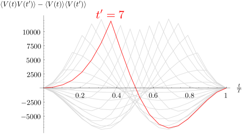
Figure 11: Volume correlation function $\langle\delta V(t)\,\delta V(t^{\prime})\rangle$ for a simulation with $T\!=\!19$, $N_{3}\!=\!70\,000$, $l_{0}\!=\!75$, and $k_{0}\!=\!1.2$. Individual curves correspond to various fixed values of $t^{\prime}$; the red curve corresponds to $\langle V(t)V(7)\rangle\!-\!\langle V(t)\rangle\langle V(7)\rangle$. The occurrence of negative values is due to the overall volume constraint.

According to the ansatz (23), the continuum operator $P^{\prime}$ is given by

$$P^{\prime}(t,t^{\prime})=\left[\frac{\partial^{2}\mathcal{L}}{\partial V^{2}}-2\,\frac{\mathrm{d}}{\mathrm{d}t}\left(\frac{\partial^{2}\mathcal{L}}{\partial V\partial\dot{V}}\right)-\frac{\mathrm{d}}{\mathrm{d}t}\left(\frac{\partial^{2}\mathcal{L}}{\partial\dot{V}^{2}}\left(\frac{\mathrm{d}}{\mathrm{d}t}\,\,\cdot\,\,\right)\right)\right]\delta(t-t^{\prime}),$$ (26)

where the partial derivatives of the Lagrangian are evaluated at $V\!=\!V_{0}(t)$. The operator $P^{\prime}$ consists of a purely diagonal part and a second-order time derivative, whose time-dependent coefficient depends only on the kinetic term in the Lagrangian.

Comparing the numerical values of the elements on the first sub- and superdiagonal of the discrete normalized operator $P^{\prime}(t,t^{\prime})$ with those on its diagonal (c.f. Fig. 12a), they differ with high accuracy by a factor of $-1/2$, as one would expect for the finite-difference representation of a second-order derivative. We conclude that the matrix $P(t,t^{\prime})$ represents a discretization of a second-order time derivative operator, like the last term in (26). The purely diagonal component of the operator appears to be absent or small compared to the second-order time derivative part. We can now try to extract the time-dependent prefactor $\partial^{2}\mathcal{L}/\partial\dot{V}^{2}[V_{0}]$ of the kinetic term $\dot{V}^{2}$ in the effective action from the simulation data. It turns out that this prefactor is very close to $1/V_{0}(t)=1/\langle V(t)\rangle$, as shown in Fig. 12b, where we have plotted the measured volume profile (solid curve) together with rescalings of the inverses of the diagonals from Fig. 12a (red and blue dots). The proportionality constant $c_{0}\approx 0.35$ has been obtained by a best fit.

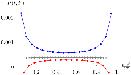
(a)

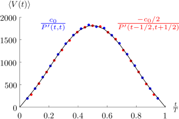
(b)

Figure 12: (a) Elements of the inverse correlation matrix $P(t,t^{\prime})$, linearly interpolated: on the diagonal (top, blue curve), on the first sub- and superdiagonal (bottom, red curve), and remaining off-diagonal elements (middle, grey; fat dots indicate accumulation of elements). (b) Volume expectation value $\langle V(t)\rangle$ (solid curve) compared to the diagonals of the normalized inverse correlation function $P^{\prime}(t,t^{\prime})\!=\!P(t,t^{\prime})\!-\!P_{0}$. The fitted proportionality constant is $c_{0}\!\approx\!0.35$.

We conclude that the volume-volume correlations are accurately described by a kinetic term in the effective action of the form

$$S[V(t)]=\int_{0}^{T}\mathrm{d}t\left(\frac{c_{0}}{2}\frac{\dot{V}^{2}}{V}+\cdots\right).$$ (27)

This kinetic term is of the same form as the one appearing in the minisuperspace action (12) (with $N=1$), up to a sign. The positive sign in (27) comes as no surprise, since the semiclassical treatment of the path integral relies on the fact that the classical solution $V_{0}(t)$ appears at a minimum of the Euclidean action. (The minisuperspace action for the spatial volume has its classical solution at a saddle point.) The reason for the sign difference of the kinetic term in the effective action extracted from the full CDT path integral can be traced back to nonperturbative “entropic” contributions coming from the number of microscopic path-integral configurations (see, for example, [12]). Their appearance in dynamically triangulated formulations of quantum gravity is generic and they play an important role in spacetime dimension $d\geq 3$ in rendering the effective action bounded from below and the Euclidean path integral stable, at least for suitably chosen bare coupling constants. In both three and four dimensions, the de Sitter universes found in the CDT approach emerge of course as minima of effective actions for the spatial volume, which differ by a sign flip from the corresponding minisuperspace actions.

This simple relation will no longer hold when other modes of the metric are included in the effective action, because the presence of a stable ground state in the extended phase of CDT quantum gravity indicates that there are no instabilities due to kinetic terms with the “wrong”, negative sign. Our current toroidal set-up has of course been designed to study effective dynamics “beyond the scale factor” and, more specifically, to determine a combined effective action of the scale factor and the global traceless degrees of the metric, the moduli $\tau_{i}$. This is the subject of a forthcoming publication [9].

7   Summary and conclusions

Motivated by the search for a larger class of observables in quantum gravity, we have initiated an investigation into three-dimensional CDT quantum gravity for universes whose spatial topology is that of a torus. Even before starting to analyze the dynamics of the global shape variables characterizing the torus geometries, we were led to consider a number of interesting issues concerning the dynamics of the volume variable only. This was triggered by the observation that typical CDT configurations on the torus with compactified time direction appear not to develop a nontrivial time dependence. In other words, unlike what happens for spherical slices, the spacetimes do not condense around a “centre of volume”, to create an extended universe on part of the time axis and a “stalk” of minimal volume everywhere else. The reason why this happens is ultimately not understood and deserves further study.

We then explored the idea of forcing the system into a nontrivial time dependence by abandoning periodic boundary conditions in time and instead using a novel type of boundary geometries, where the spatial tori degenerate into one-dimensional circles of a given length. Invoking a minisuperspace picture, we searched for a set of classical gravitational solutions in the continuum, with the same type of boundary conditions and depending on the same number of free variables as the CDT system, to serve as a reference point for identifying certain classical features of the continuum limit of the latter. This led us to a generalized minisuperspace model, where (in ADM language) the Hamiltonian constraint is not required to vanish. We found that measurements of the CDT volume profiles for a wide range of boundary lengths and values of the inverse Newton coupling $k_{0}$ can be matched with good quality to solutions derived in this generalized minisuperspace model. However, with the wide range of shapes available as classical volume profiles, this is perhaps not too surprising. Also, an asymmetric choice of boundary conditions in the simulations did not yield the result expected from the minisuperspace comparison. At this point, it is difficult to disentangle whether this is due to insufficient system size or insufficient “classicality” (large quantum fluctuations), or whether perhaps our identification of discrete proper time and boundary lengths with the corresponding continuum quantities may have been too naïve. The analysis of the dynamics of the moduli [9] will shed some light on the size of quantum fluctuations and the degree to which scale and shape are dynamically coupled.

As we have already commented in Sec. 2, the general issue of boundary conditions of the nonperturbative path integral, their relation with a continuum Hilbert space and ultimately classical interpretation is highly nontrivial. Comparing with 1+1 dimensional CDT quantum gravity, where the corresponding Hilbert space construction is under complete analytical control [28], the situation in higher dimension is much more involved. Despite our choice of particularly simple “collapsed” boundary conditions in 2+1 dimensions, we saw in Sec. 5 that subtleties remain. We observed a clear effect of the boundary conditions on the bulk behaviour of the volume variable, but to isolate the influence of the boundary from other effects would require a more systematic analysis, where bulk and boundary are scaled simultaneously at a specified relative rate, similar to what can be done in CDT in 1+1 dimensions to obtain a spacetime of anti-de Sitter type [29]. This is an interesting issue, but beyond the scope of this paper.

With the minisuperspace comparison remaining at this stage somewhat inconclusive, we turned to a more direct determination of the effective action for the spatial volume from the simulation data. Here, our method of extracting it from inverting the measured matrix of volume-volume correlation worked beautifully, and gave an unambiguous result of the expected form for the kinetic term, which coincides with that found in the spherical case. – This concludes the first part of our investigation into the nonperturbative CDT description of 2+1 dimensional quantum gravity on a torus. A natural next step will be a similar analysis of the dynamics of the moduli parameters of the same system, involving a new set of observables relating to the global shape of the quantum universe.

Acknowledgments. This work was supported by the Netherlands Organisation for Scientific Research (NWO) under their VICI program. T.G. Budd acknowledges support through the ERC-Advanced Grant 291092, “Exploring the Quantum Universe” (EQU). Research at Perimeter Institute is supported by the Government of Canada through Industry Canada and by the Province of Ontario through the Ministry of Economic Development and Innovation. Both authors acknowledge support from Utrecht University, where part of this work was done.

References

- [1] Y. Watabiki: Analytic study of fractal structure of quantized surface in two-dimensional quantum gravity, Prog. Theor. Phys. Suppl. 114 (1993) 1; J. Ambjørn and Y. Watabiki: Scaling in quantum gravity, Nucl. Phys. B 445 (1995) 129 [hep-th/9501049]; J. Ambjørn, J. Jurkiewicz and Y. Watabiki: On the fractal structure of two-dimensional quantum gravity, Nucl. Phys. B 454 (1995) 313 [hep-lat/9507014].
- [2] J. Ambjørn, A. Görlich, J. Jurkiewicz and R. Loll: Nonperturbative quantum gravity, Phys. Rept. 519 (2012) 127 [arXiv:1203.3591, hep-th].
- [3] J. Ambjørn, J. Jurkiewicz and R. Loll: Emergence of a 4D world from causal quantum gravity, Phys. Rev. Lett. 93 (2004) 131301 [hep-th/0404156].
- [4] J. Ambjørn, J. Jurkiewicz and R. Loll: Reconstructing the universe, Phys. Rev. D 72 (2005) 064014 [hep-th/0505154].
- [5] J. Ambjørn, J. Jurkiewicz and R. Loll: Spectral dimension of the universe, Phys. Rev. Lett. 95 (2005) 171301 [hep-th/0505113].
- [6] J. Ambjørn, A. Görlich, J. Jurkiewicz and R. Loll: Planckian birth of the quantum de Sitter universe, Phys. Rev. Lett. 100 (2008) 091304 [arXiv:0712.2485, hep-th], The nonperturbative quantum de Sitter universe, Phys. Rev. D 78 (2008) 063544 [arXiv:0807.4481, hep-th].
- [7] J. Ambjørn, J. Jurkiewicz and R. Loll: Nonperturbative 3-d Lorentzian quantum gravity, Phys. Rev. D 64 (2001) 044011 [hep-th/0011276].
- [8] J. Ambjørn, J. Barkley and T.G. Budd: Roaming moduli space using dynamical triangulations, Nucl. Phys. B 858 (2012) 267 [arXiv:1110.4649, hep-th].
- [9] T.G. Budd and R. Loll, to appear.
- [10] J. Ambjørn, S. Jordan, J. Jurkiewicz and R. Loll: A second-order phase transition in CDT, Phys. Rev. Lett. 107 (2011) 211303 [arXiv:1108.3932, hep-th], Second- and first-order phase transitions in CDT, Phys. Rev. D 85 (2012) 124044 [arXiv:1205.1229, hep-th].
- [11] S. Carlip: Quantum gravity in 2+1 dimensions, Cambridge University Press, Cambridge, UK (1998), Quantum gravity in 2+1 dimensions: The case of a closed universe, Living Rev. Rel. 8 (2005) 1 [gr-qc/0409039].
- [12] J. Ambjørn, A. Görlich, J. Jurkiewicz and R. Loll: CDT - an entropic theory of quantum gravity [arXiv:1007.2560, hep-th].
- [13] J. Ambjørn, J. Jurkiewicz and R. Loll: Dynamically triangulating Lorentzian quantum gravity, Nucl. Phys. B 610 (2001) 347 [hep-th/0105267].
- [14] J. Ambjørn, J. Jurkiewicz and R. Loll: Lorentzian and Euclidean quantum gravity: Analytical and numerical results, in Proceedings of M-theory and quantum geometry, eds. L. Thorlacius et al., (Kluwer, 2000) 382-449 [hep-th/0001124], Quantum gravity, or The art of building spacetime, in Approaches to quantum gravity, ed. D. Oriti (Cambridge University Press, Cambridge, UK, 2009) 341-359 [hep-th/0604212], Causal dynamical triangulations and the quest for quantum gravity, in Foundations of space and time, eds. G. Ellis, J. Murugan and A. Weltman (Cambridge University Press, Cambridge, UK, 2012) [arXiv:1004.0352, hep-th]; R. Loll: The emergence of spacetime or quantum gravity on your desktop, Class. Quant. Grav. 25 (2008) 114006 [arXiv:0711.0273, gr-qc]; J. Ambjørn, A. Görlich, J. Jurkiewicz and R. Loll: Quantum gravity via Causal Dynamical Triangulations [arXiv:1302.2173, hep-th].
- [15] S. Jordan and R. Loll: Causal Dynamical Triangulations without preferred foliation [arXiv:1305.4582, hep-th].
- [16] D. Benedetti and J. Henson: Spectral geometry as a probe of quantum spacetime, Phys. Rev. D 80 (2009) 124036 [arXiv:0911.0401, hep-th].
- [17] R. Kommu: A validation of Causal Dynamical Triangulations, Class. Quant. Grav. 29 (2012) 105003 [arXiv:1110.6875, gr-qc].
- [18] J. Ambjørn, J. Jurkiewicz and R. Loll: 3-d Lorentzian, dynamically triangulated quantum gravity, Nucl. Phys. Proc. Suppl. 106 (2002) 980 [hep-lat/0201013].
- [19] M.K. Sachs: Testing lattice quantum gravity in 2+1 dimensions [arXiv: 1110.6880, gr-qc].
- [20] C. Anderson, S.J. Carlip, J.H. Cooperman, P. Horava, R.K. Kommu and P.R. Zulkowski: Quantizing Hořava-Lifshitz gravity via Causal Dynamical Triangulations, Phys. Rev. D 85 (2012) 044027 [arXiv:1111.6634, hep-th].
- [21] J. Ambjørn, J. Jurkiewicz, R. Loll and G. Vernizzi: Lorentzian 3-D gravity with wormholes via matrix models, JHEP 0109 (2001) 022 [hep-th/0106082], 3-D Lorentzian quantum gravity from the asymmetric ABAB matrix model, Acta Phys. Polon. B 34 (2003) 4667 [hep-th/0311072]; J. Ambjørn, J. Jurkiewicz and R. Loll: Renormalization of 3-d quantum gravity from matrix models, Phys. Lett. B 581 (2004) 255 [hep-th/0307263].
- [22] D. Benedetti, R. Loll and F. Zamponi: (2+1)-dimensional quantum gravity as the continuum limit of Causal Dynamical Triangulations, Phys. Rev. D 76 (2007) 104022 [arXiv:0704.3214, hep-th].
- [23] B. Dittrich and R. Loll: A hexagon model for 3-D Lorentzian quantum cosmology, Phys. Rev. D 66 (2002) 084016 [hep-th/0204210].
- [24] A. Hatcher: Algebraic topology, Cambridge University Press, Cambridge, UK (2002).
- [25] V. Moncrief: Reduction of the Einstein equations in (2+1)-dimensions to a Hamiltonian system over Teichmüller space, J. Math. Phys. 30 (1989) 2907.
- [26] P.O. Mazur and E. Mottola: The gravitational measure, solution of the conformal factor problem and stability of the ground state of quantum gravity, Nucl. Phys. B 341 (1990) 187.
- [27] A. Dasgupta and R. Loll: A proper time cure for the conformal sickness in quantum gravity, Nucl. Phys. B 606 (2001) 357 [hep-th/0103186].
- [28] J. Ambjørn and R. Loll: Nonperturbative Lorentzian quantum gravity, causality and topology change, Nucl. Phys. B 536 (1998) 407 [hep-th/9805108].
- [29] J. Ambjørn, R. Janik, W. Westra and S. Zohren: The emergence of background geometry from quantum fluctuations, Phys. Lett. B 641 (2006) 94 [gr-qc/0607013].