Binding carriers to a non-magnetic impurity in a two-dimensional square Ising antiferromagnet

Abstract

A hole in a two-dimensional Ising antiferromagnet was believed to be infinitely heavy due to the string of wrongly oriented spins it creates as it moves, which should trap it near its original location. Trugman showed that, in fact, the hole acquires a finite effective mass due to contributions from so-called Trugman loop processes, where the hole goes nearly twice around closed loops, first creating and then removing wrongly-oriented spins, and ending up at a different lattice site. This generates effective second- and third-nearest-neighbor hopping terms which keep the quasiparticle on the sublattice it was created on. Here, we investigate the trapping of the quasiparticle near a single attractive non-magnetic impurity placed at one lattice site. We consider the two cases with the quasiparticle and impurity being on the same versus on different sublattices. The main result is that even though the quasiparticle can not see the bare disorder in the latter case, the coupling to magnons generates an effective renormalized disorder on its own sublattice which is strong enough to lead to bound states, which however have a very different spectrum than when the quasiparticle and impurity are on the same sublattice.

I introduction

Understanding the motion of charge carriers in a two-dimensional (2D) Heisenberg antiferromagnet (AFM) is a central challenge for deciphering the mechanism behind high-temperature superconductivity in cuprates.Kane ; Frank ; Sachdev ; Chubukov ; Sigia At half-filling, the strong hybridization $t_{pd}$ between copper $d_{x^{2}-y^{2}}$ and oxygen $p_{x,y}$ orbitals drives the CuO₂ planes into an insulating state in which the holes on neighboring copper atoms align their spins antiferromagnetically in order to gain the superexchange energy $\mathrm{J}\sim t_{pd}^{4}/\Delta^{3}$, where $\Delta=E_{p}-E_{d}$ is the charge transfer energy from $d$ to $p$ orbitals. Superconductivity emerges upon doping the 2D AFM planes with charge carriers.Lee ; Phillips

A major setback in the search for an analytic description of the behavior of these charge carriers is the lack of a simple wave function for the ground state of the undoped AFM planes. The semi-classical Néel state breaks spin rotation symmetry and is therefore smeared out by quantum spin fluctuations to a significant degree that is hard to capture with simple wave functions. This leaves numerical calculations as the only way to make quantitative predictions.Dagotto While implementing such numerical calculations is already a complicated task even for a clean system, a further complication comes from the presence of disorder and imperfections in the real materials, introduced during the sample growth and preparation. Given the low dimensionality, even weak disorder may have dramatic effects on the motion of charge carriers in the CuO₂ planes. It is well known that non-magnetic impurities are strong pair breakers in $d$-wave superconductors.Riera0 Indeed, substitution of only a few percent of the copper atoms with non-magnetic impurities has been observed to suppress the superconductivity by localizing the low-energy electronic states.basov Even in the cleanest samples, the dopant ions are in close proximity to the CuO₂ planes, and the disorder potential they create can disturb the motion of the charge carriers.

Impurities have been shown to be responsible for a range of phenomena in low-dimensional correlated electron systems, and they can be also utilized for probing correlations which are otherwise difficult to observe in the ground state.Alloul For the undoped parent compound, mean-field analysis of the disordered Hubbard model predicts the emergence of an inhomogeneous metallic phase in which the Mott gap is locally closed wherever the disorder is strong enough to do so.Heidarian However, it is not always the case that impurities destroy the order in the underlying system. For instance, impurities induce local magnetic order in one-dimensional (1D) quantum magnets,Suchaneck and long-range antiferromagnetism is predicted upon doping some quantum spin liquids with nonmagnetic impurities.wessel In any event, a complete understanding of the interplay between disorder and AFM correlations and especially of their role in controlling the carrier dynamics away from half-filling is still lacking.

In this paper, we consider a much simpler variant of this problem where, at zero temperature, a hole is created in a 2D Ising AFM on a square lattice, and is also subject to the on-site attractive potential of an impurity that can be visited by the hole. Thus, our model is very different from previous models of an impurity in a 2D Heisenberg AFM, which assumed that the hole cannot visit the impurity site, and is coupled to it at most through exchange.Poilblanc1 ; Poilblanc2 As we discuss in the following, our results have some similarities but also considerable differences from those obtained numerically in these other models.

We investigate the local density of states (LDOS) near the impurity to study the appearance of bound states, focusing specifically on the relevance of the magnetic sublattice on which the impurity is located. The advantage of our approach is that the wave function of the undoped 2D AFM is the simple Néel state, and this allows us to study the problem (quasi)analytically. Of course, spin fluctuations are completely absent, but, as we argue in our discussion, our results allow us to speculate about (at least some of) their likely effects.

We note that a single hole in an Ising AFM was initially believed to be localized even in the absence of impurities, because when the hole hops it reshuffles the spins along its path, thus creating a string of wrongly oriented spins. In dimensions larger than one, the energy cost of this string increases roughly linearly with its length, resulting in an effective potential well that binds the hole in the vicinity of its original position. Finite mobility was believed to arise only due to spin fluctuations which can remove pairs of such defects,Brink ; Poilblanc3 but they are absent from the Ising Hamiltonian.

However, as pointed out by Trugman,Trugman the hole is actually delocalized even in the Ising AFM, and it achieves this by going twice around closed loops. The string of misaligned spins that are created in the first round is removed when spins are reshuffled again during the second round. When the last one is removed, the hole ends up at a different site from where it started, and by repeating this process it can move anywhere on its original sublattice (spin conservation ensures that the hole propagates on one sublattice). This raises the question of how the hole’s motion will be affected by an attractive impurity, especially by one located on the other sublattice than the one on which the hole resides. While one expects the hole to become bound to the impurity if they are on the same sublattice, if they are on different sublattices, one may expect the hole not to be sensitive to the presence of the impurity and therefore remain unbound. We investigate this problem using a variational method introduced in Ref. Mona, to study the clean case, which we generalize here to systems that are not invariant under translations. Our results confirm the expected existence of a bound state when the hole and impurity are on the same sublattice. When they are on different sublattices, we find that the naive picture described above is wrong: the hole develops multiple bound states with a characteristic spectrum and symmetries. The implications of these results as seen in the wider context of the effect of disorder on dressed quasi-particles are also discussed.

This paper is organized as follows: we introduce the model in Sec. II. The generalization of the variational method to inhomogeneous systems is discussed in Sec. III, followed in Sec. IV by results for a single impurity located (i) on the same, and (ii) on the other sublattice than the hole. We conclude the paper by giving a summary and discussing possible further developments of this work in Sec. V.

II model

We consider the motion of a single hole doped into a spin-$1/2$ Ising antiferromagnet on a 2D square lattice. The Hamiltonian of the undoped system is

$${\cal{H}}_{\mathrm{AFM}}=\mathrm{J}\sum_{<i,j>}[S_{i}^{z}S_{j}^{z}+\frac{1}{4}]=\mathrm{\bar{J}}\sum_{<i,j>}[\sigma_{i}^{z}\sigma_{j}^{z}+1],$$ (1)

where $\sigma^{z}$ is the Pauli matrix and $\mathrm{\bar{J}}=\mathrm{J}/4>0$. The vacuum $|0\rangle$ is the Néel-ordered state, with all spins on one sublattice pointing up and those on the other sublattice pointing down. Excitations are gapped spin-flips, or localized magnons, and we refer to them also as spin defects. The creation operator for a spin defect is written in terms of the spin raising and lowering operators, $\sigma^{\pm}=\sigma^{x}\pm i\sigma^{y}$:

$$d^{\dagger}_{i}=\begin{cases}\sigma_{i}^{-}&\text{if\,\,\,\,\, }i\in\uparrow\mathrm{sublattice},\\ \sigma_{i}^{+}&\text{if\,\,\,\,\, }i\in\downarrow\mathrm{sublattice}.\end{cases}$$ (2)

Consider now the doped case. Creating a hole in this system corresponds to removing a spin from the same lattice site, therefore the hole creation operators are:

$$h^{\dagger}_{i}=\begin{cases}c_{i\uparrow}&\text{if\,\,\,\,\, }i\in\uparrow\mathrm{sublattice},\\ c_{i\downarrow}&\text{if\,\,\,\,\, }i\in\downarrow\mathrm{sublattice}.\end{cases}$$ (3)

Once the hole is created ($h_{i}^{\dagger}$), it moves via nearest-neighbor hopping. This, however, either creates a spin defect on the hole’s departure site ($d^{\dagger}_{i}$) or annihilates one from its arrival site ($d_{j}$), if there was a spin defect already there. The Hamiltonian can therefore be written as:Mona

$${\cal{H}}={\cal{P}}\{-t\sum_{<ij>}[h_{j}^{\dagger}h_{i}(d^{\dagger}_{i}+d_{j})+\mathrm{H.c.}]\}{\cal{P}}+{\cal{H}}_{\mathrm{AFM}}-Uh^{\dagger}_{0}h_{0},$$ (4)

where ${\cal{P}}$ is the projection operator enforcing no double occupancy: at any site there is a hole or there is a spin which is either properly oriented or is flipped, $h_{i}^{\dagger}h_{i}+d_{i}^{\dagger}d_{i}+d_{i}d_{i}^{\dagger}=1$. Thus, the first term describes the hopping of the hole which is accompanied by either spin defect creation or annihilation.

In addition, there is an attractive potential of strength $U$ centered at the origin $\bf r=0$, which changes the on-site energy of the visiting hole (variations of the local hoppings and exchanges can be trivially included in the model and our solution, but should not lead to any qualitative changes if they are small or moderate in size). Physically, such a potential can be due to an attractive non-magnetic impurity located above the origin, in a different layer, and which modulates the on-site energy at the origin. Another possibility comes from replacing the atom at the origin by an impurity atom with the same valence, but whose orbitals lie at lower energies than those of the background atoms. This is very different from the impurity models studied in previous work where the impurity is an inert site that can not be visited by carriers, Poilblanc1 and there is at most exchange between the spin of the impurity and that of carriers located on neighboring sites.Poilblanc2

III Propagation of the hole in the clean system

In this section, we construct the equations of motion for the zero-temperature Green’s function (GF) of a single hole moving through the lattice in the absence of impurity, $U=0$. This was done using a momentum-space formulation in Ref. Mona, . Here, we present a real-space derivation, whose use becomes inevitable once we introduce the impurity which breaks the translational invariance. The single hole GF is defined as

$$G_{\bf 0,R}(\omega)=\langle\mathrm{0}|h_{\bf 0}\hat{G}(\omega)h^{\dagger}_{\bf R}|\mathrm{0}\rangle,$$ (5)

where $\hat{G}(\omega)=\lim_{\eta\rightarrow 0^{+}}1/(\omega-{\cal H}+i\eta)$ is the resolvent associated with the Hamiltonian when $U=0$.

By dividing the Hamiltonian as ${\cal H}={\cal H}_{\mathrm{AFM}}+{\cal H}_{t}$ where ${\cal H}_{t}$ is the first term in Eq. (4) responsible for hopping, equations of motion for $G_{\bf 0,R}(\omega)$ can be generated by repeated use of the Dyson identity

$$\hat{G}(\omega)=\hat{G}_{\mathrm{AFM}}(\omega)+\hat{G}(\omega){\cal H}_{t}\hat{G}_{\mathrm{AFM}}(\omega),$$

in which $\hat{G}_{\mathrm{AFM}}(\omega)=\lim_{\eta\rightarrow 0^{+}}1/(\omega-{\cal H}_{\mathrm{AFM}}+i\eta)$. Using this, Eq. (5) becomes

$$G_{\bf 0,R}(\omega)=g_{0}(\omega)[\delta_{\bf 0,R}-t\sum_{\bf u}F_{1}(\bf R,u;\omega)],$$ (6)

where $g_{0}(\omega)=1/(\omega-4\mathrm{\bar{J}}+i\eta)$ and $4\mathrm{\bar{J}}$ is the cost of breaking four AFM bonds when introducing the hole in the lattice. Here the lattice constant is set to unity, $a=1$, ${\bf u=\pm x,\pm y}$ is any of the four nearest-neighbor vectors and $F_{1}({\bf R},{\bf u};\omega)=\langle 0|h_{\bf 0}\hat{G}(\omega)d^{\dagger}_{\bf R}h^{\dagger}_{\bf R+u}|0\rangle$ has the hole at a nearby site ${\bf R+u}$ and a spin defect at ${\bf R}$. To simplify notation, from now on we do not write explicitly the dependence on $\omega$ of all these GFs.

The equation of motion for $F_{1}$ can be similarly generated. Upon application of the Dyson identity, the hole can hop back to ${\bf R}$ and remove the spin defect, or it can hop further away and create a second spin defect, with an associated GF $F_{2}$, and so on. As discussed, states with many spins defects are less likely to occur due to the energy cost of creating the spin defects. In order to avoid the rise in the number of spin defects, the hole can trace back its path to remove the spin defects, however this effectively confines the hole to the vicinity of its creation site. The hole is freed to move on the lattice by the so-called Trugman loop processes in which it goes twice around a closed path. In this case, spin defects that are created at the first pass are annihilated when the hole arrives there the second time. Furthermore, when the very last spin defect is annihilated, the hole ends up two hops away from its starting point, which is equivalent to either second- or third-nearest-neighbor hopping on the main lattice (i.e., first- or second-nearest-neighbor hopping on the hole’s sublattice).

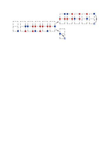
Figure 1: Effective first- and second-nearest-neighbor hoppings of the hole (the blue square) achieved with loops involving only up to three spin defects. The latter is realized when the hole starts a second loop before removing the last spin defect it created during the first loop. The spin defects are shown by red circles. The properly oriented spins are not shown.

Longer loops involve more costly intermediate states with more spin defects, therefore we can proceed within a variational approach in which a limit is set for the maximum number of spin defects that can be generated as the hole propagates. We choose to work with up to three spin-defects, which is the minimum number necessary for the hole to complete the shortest possible loop. Moreover, we only keep spin defect configurations consistent with these short closed loops (i.e., we exclude, for example, configurations where all three spin defects are collinear). Figure 1 shows how both types of effective hoppings can be generated with the three spin defects types of configurations that we keep in our variational calculation. One can include more configurations with numerical simulations, but this was shown to results in only quantitative differences as long as $t/\mathrm{J}$ is not too large.Riera ; Mona

Coming back to the equation of motion for $F_{1}$, it relates it to $G_{\bf 0,R}(\omega)$ and also to three GSs $F_{2}$ with two spin defects. One of these, with the two spin defects collinear with the hole, cannot lead to a closed loop without generating more than three spin defects, therefore we exclude it from the variational space, as discussed. Hence, we are left with only three terms

$$F_{1}({\bf R,u})=-tg_{1}[G_{\bf 0,R}+\sum_{\bf v\perp u}F_{2}({\bf R,u,v})],$$ (7)

where $F_{2}({\bf R},{\bf u},{\bf v})=\langle 0|h_{\bf 0}\hat{G}(\omega)d^{\dagger}_{\bf R}d^{\dagger}_{\bf R+u}h^{\dagger}_{\bf R+u+v}|0\rangle$, ${\bf v}=\pm{\bf x}$ if ${\bf u}\in\{{\bf y,-y}\}$ and vice versa, $g_{1}=1/(\omega-10\mathrm{\bar{J}}+i\eta)$ and $10\mathrm{\bar{J}}$ is the cost of having a spin defect near the hole.

Within our variational space, the equation of motion for $F_{2}$ is

$$F_{2}({\bf R,u,v})=-tg_{2}[F_{1}({\bf R,u})+F_{3}({\bf R,u,v,-u})],$$ (8)

where

$$F_{3}({\bf R},{\bf x},{\bf y},{\bf z})=\langle 0|h_{\bf 0}\hat{G}(\omega)d^{\dagger}_{\bf R}d^{\dagger}_{\bf R+x}d^{\dagger}_{\bf R+x+y}h^{\dagger}_{\bf R+x+y+z}|0\rangle$$

and $g_{2}=1/(\omega-14\mathrm{\bar{J}}+i\eta)$, where $14\mathrm{\bar{J}}$ is the cost of the allowed two spin-defects configurations. The other two three spin-defect configurations that can be reached starting from $d^{\dagger}_{\bf R}d^{\dagger}_{\bf R+u}h^{\dagger}_{\bf R+u+v}|0\rangle$ do not belong to our variational space and are discarded. Finally, in this variational space $F_{3}$ relates to $F_{2}$ only

$$F_{3}({\bf R},{\bf u},{\bf v},{\bf-u})=\\ -tg_{3}[F_{2}({\bf R,u,v})+F_{2}({\bf R+u+v,-v,-u})],$$ (9)

with $g_{3}=1/(\omega-16\mathrm{\bar{J}}+i\eta)$, $16\mathrm{\bar{J}}$ being the energy of the allowed three-spin-defect configurations.

These equations can be used to eliminate all $F_{3},F_{2},F_{1}$ unknowns and be left with equations involving only $G_{\bf 0,R}(\omega)$. The details are presented in the Appendix. The final results is:

$$G_{\bf 0,R}(\omega)=\bar{g}_{0}(\omega)[\delta_{\bf R,0}\\ -t_{1}(\omega)\sum_{{\bf\boldsymbol{\delta}}}G_{\bf 0,R+{\boldsymbol{\delta}}}(\omega)-t_{2}(\omega)\sum_{{\boldsymbol{\xi}}}G_{\bf 0,R+\boldsymbol{\xi}}(\omega)],$$ (10)

in which $\bar{g}_{0}(\omega)=1/(\omega-4\mathrm{\bar{J}}+4t\zeta_{1}(\omega)+i\eta)$, $t_{1}(\omega)=2t\zeta_{3}(\omega)$, $t_{2}(\omega)=t\zeta_{2}(\omega)$ and $\boldsymbol{\delta}={\bf\pm u\pm v}$ and $\boldsymbol{\xi}={\pm 2\bf u}$ are all the second- and third-nearest-neighbor vectors of the full lattice, respectively. The explicit expressions of the $\zeta$ functions are given in the Appendix.

Equation (10) shows that the motion of the hole is similar to that of a quasiparticle with effective second- and third-nearest-neighbor hoppings $t_{1}(\omega)$ and $t_{2}(\omega)$, respectively, and an effective on-site energy $\varepsilon(\omega)=4\mathrm{\bar{J}}-4t\zeta_{1}(\omega)$. This quasiparticle is comprised of the hole accompanied by a cloud of spin defects which are constantly created and annihilated, helping to release the quasiparticle to move freely on the lattice. Note that all sites ${\bf R}$, ${\bf R+\boldsymbol{\delta}}$, and ${\bf R+\boldsymbol{\xi}}$ belong to the same sublattice. Therefore, the quasiparticle propagates on the sublattice on which the hole is originally introduced, and for which $\boldsymbol{\delta}$ and $\boldsymbol{\xi}$ are the first- and second-nearest-neighbor vectors, respectively. The constraint that keeps the quasiparticle moving on one sublattice is very general, being due to the spin-conserving nature of the Hamiltonian which prevents the hole from ending up on the other sublattice in the absence of spin defects: if the hole starts on one sublattice and ends up on the other one, the $z$ component of the total spin angular momentum of the system changes from $S^{z}_{i}=\pm 1/2$ to $S^{z}_{f}=\mp 1/2$, therefore there needs to be an odd number of spin defects around to compensate for the change of spin $S_{f}^{z}-S_{i}^{z}=\mp 1$.

Before presenting the real-space solution of Eq. (10), note that we are now in a position to construct the momentum-space Green’s function:

$$G({\bf k};\omega)=\langle\mathrm{0}|h_{\bf k}\hat{G}(\omega)h^{\dagger}_{\bf k}|\mathrm{0}\rangle=\frac{1}{\omega+i\eta-\epsilon(\omega;{\bf k})},$$ (11)

where $h_{\bf k}=\sum_{\bf r}\exp(-i{\bf k\cdot{\bf r}})h_{\bf r}/\sqrt{\bar{N}}$ and the sum is over the sites in the hole’s sublattice and $\bar{N}\rightarrow\infty$ is their number. $\epsilon(\omega;{\bf k})$ is the self-energy coming from coupling to the spin degrees of freedom, which is responsible for the dynamical generation of the hole’s energy dispersion:

$$\epsilon(\omega;{\bf k})=\varepsilon(\omega)-2t_{1}(\omega)[\cos(k_{x}+k_{y})+\cos(k_{x}-k_{y})]\\ -2t_{2}(\omega)[\cos(2k_{x})+\cos(2k_{y})].$$ (12)

As required, this is identical to the solution derived using a momentum space formalism in Ref. Mona, .typo The spectral function $A({\bf k};\omega)=-\mathrm{Im}G({\bf k};\omega)/\pi$ is then used to identify the quasiparticle excitations and their various properties such as energy dispersion, effective mass, etc.Mona

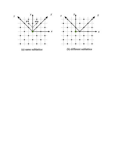
Figure 2: (Color online) The choice of coordinate systems for the lattice with impurity. The impurity, shown in green, is at the origin of the $xy$ axes that span the original lattice with unit vectors ${\bf x,y}$. The $XY$ axes are rotated by $45\,^{\circ}$ and span the sublattice (black dots) on which the quasiparticle propagates via the elementary vectors ${\bf y\pm x}$.

Equation (10) can be solved directly in real space by the method of continued fractions detailed in Ref. Mirko, . For completeness, we briefly outline it here. Let $n$ and $m$ be the $x$ and $y$ components of ${\bf R}\neq{\bf 0}$ on the coordinates axes $XY$ which is rotated by $45\,^{\circ}$ with respect to the lattice. It spans the sublattice on which the quasiparticle moves, shown by the black dots in Fig. 2(a); its elementary vectors are ${\bf y\pm x}$. In this coordinate system, Eq. (10) can be written as

$$G_{n,m}=\bar{g}_{0}[-t_{1}(G_{n+1,m}+G_{n-1,m}+G_{n,m+1}+G_{n,m-1})\\ -t_{2}(G_{n+1,m+1}+G_{n+1,m-1}+G_{n-1,m+1}+G_{n-1,m-1})],$$ (13)

where $G_{n,m}\equiv G_{\bf 0,R}(\omega)$ for ${\bf R}=n({\bf y+x})+m({\bf y-x})$ is a shorthand notation. Eq. (13) can be expressed as a single-index recursive relation by grouping distinct GF’s with $n\geq m\geq 0$ into column vectors $V_{M}$ according to their Manhattan distance $M=n+m$:

$$V_{M=2r}=\begin{pmatrix}G_{2r,0}\\ G_{2r-1,1}\\ \vdots\\ G_{r,r}\end{pmatrix},V_{M=2r-1}=\begin{pmatrix}G_{2r-1,0}\\ G_{2r-2,1}\\ \vdots\\ G_{r,r-1}\end{pmatrix}.$$

These are the only distinct GFs since all others can be related to these using symmetries: $G_{n,m}=G_{m,n}=G_{n,-m}=G_{-n,m}$, etc. In terms of these vectors, Eqs. (13) be grouped into the following matrix form

$$\lambda_{r}V_{r}=\tilde{\alpha}_{r}V_{r-2}+\alpha_{r}V_{r-1}+\beta_{r}V_{r+1}+\tilde{\beta}_{r}V_{r+2}$$ (14)

for $r\geq 2$ and

$$\begin{array}[]{rcl}V_{0}&=&\bar{g}_{0}(\omega)+\beta_{0}V_{1}+\beta_{0}V_{2}\\ V_{1}&=&\alpha_{1}V_{0}+\beta_{1}V_{2}+\tilde{\beta}_{1}V_{3}\end{array}$$ (15)

for the GFs with $M=0,1$. Here, $\lambda$, $\tilde{\alpha}$, $\alpha$, $\beta$ and $\tilde{\beta}$ are extremely sparse matrices whose elements can be read from Eq. (13). Combining two copies of Eq. (14) corresponding to $r=2s-1$ and $r=2s$ leads to:

$$\Gamma_{s}W_{s}=A_{s}W_{s-1}+B_{s}W_{s+1},$$ (16)

where $W_{s}=\begin{pmatrix}V_{2s-1}\\ V_{2s}\end{pmatrix}$, $\Gamma_{s}=\begin{pmatrix}\lambda_{2s-1}&-\beta_{2s-1}\\ -\alpha_{2s}&\lambda_{2s}\end{pmatrix}$, etc. Because Eq. (16) links three consecutive terms, it can be solved in terms of continued fractions of matrices. Specifically, assuming a solution as $W_{s}=\Omega_{s}W_{s-1}$ and using it in Eq. (16) gives

$$\Omega_{s}=(\Gamma_{s}-B_{s}\Omega_{s+1})^{-1}A_{s},$$ (17)

which can be calculated starting from a cutoff $c$ such that $\Omega_{c+1}=0$. This results in a continued-fraction solution for $\Omega_{s}$. In particular, this gives $\Omega_{2}$ which relates $W_{2}$ (set of $V_{3}$ and $V_{4}$) to $W_{1}$ (set of $V_{1}$ and $V_{2}$). Finally, the diagonal element of Green’s function is found by using these in Eqs. (15) and (14) with $r=2$ to solve for $V_{0}=G_{0,0}(\omega)$ from which we find the hole’s local density of states (LDOS):

$$\rho({\bf r};\omega) =-\frac{1}{\pi}\mathrm{Im}\langle 0|h_{\bf r}\hat{G}(\omega)h^{\dagger}_{\bf r}|0\rangle$$ (18)

$$=-\frac{1}{\pi}\mathrm{Im}G_{0,0}(\omega),$$

which is same as the total density of states in the clean system. Other GFs $G_{0,{\bf r\neq 0}}(\omega)$ can be then calculated from $G_{0,0}(\omega)$ using the continued fraction matrices $\Omega_{s}$. In practice, the calculation is done on a finite lattice which is chosen sufficiently large that the GFs become negligible beyond its boundaries (the broadening $\eta$ introduces an effective lifetime $1/\eta$ that prevents the quasiparticle from going arbitrarily far away from its original location). Note that the equations are modified for the lattice sites close to the boundary: if the hole can not hop outside the boundary, some of the generalized GS $F_{1},F_{2},F_{3}$ must be set to zero for sites close to the boundary, resulting in modified effective hoppings $t_{1}(\omega),t_{2}(\omega)$, and on-site energy $\varepsilon(\omega)$ near the boundary. If the cutoff is large enough, however, the solution becomes insensitive to these changes.

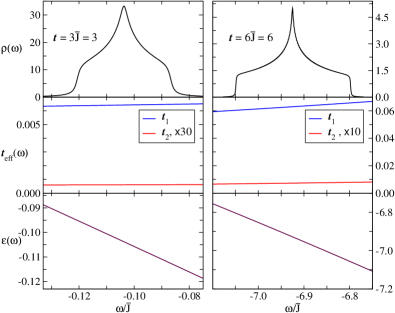
Figure 3: (Color online) The total density of states (top panels), effective hoppings $t_{1}(\omega),t_{2}(\omega)$ (middle panels) and on-site energy $\varepsilon(\omega)$ (bottom panels) in the clean system for two different values of $t/\mathrm{\bar{J}}$. The effective parameters are relatively constant within the energy band, explaining why the DOS has the generic form expected for a bare particle with nearest-neighbor hopping on a square lattice. Here $\mathrm{\bar{J}}=1$, $\eta=10^{-3}$ and $\mathrm{t}=3$ (left panels) and $\mathrm{t}=6$ (right panels), respectively.

The top panels in Fig. 3 show the hole’s total density of states (DOS) at two moderate $t/J$ values, for which this variational approximation was shown to be in good agreement with the numerical results.Mona The quasiparticle bandwidth for $t=6$ is considerably larger than that for $t=3$, showing the rapid decrease of the quasiparticle’s effective mass with increasing hopping. In the lower panels we plot the quasiparticle’s effective hoppings $t_{1}(\omega),t_{2}(\omega)$ and on-site energy $\varepsilon(\omega)$ over this energy range. It shows that their energy dependence is relatively weak in this range and that $t_{2}(\omega)$, which would make the DOS asymmetric, is vanishingly small. This explains why the quasiparticle, in spite of being dressed with magnons, has a DOS similar to that of a featureless bare particle with only a constant first-nearest-neighbor hopping.

IV The effect of the impurity

In the previous section we confirmed that the hole’s motion in the clean system is described by an effective tight-binding Hamiltonian with second- and third-nearest-neighbor hoppings which keep the quasiparticle on the same sublattice at all times. In this section we investigate the effect of an attractive impurity on the spectrum of the quasiparticle. The impurity can be on the sublattice in which the quasiparticle moves, or it can be on the other sublattice. In the former case, one expects the quasiparticle to bind to the impurity. As mentioned in the introduction, when they are on different sublattices one might naively expect the quasiparticle to remain mobile and insensitive to the presence of impurity. However, we will see that this is not the case.

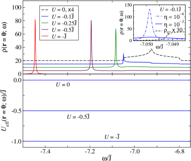
Figure 4: (Color online) (Top) LDOS at the impurity site for various values of $U$. The dashed line is the DOS in the clean system, times 4. At finite $U$, a single bound state splits from the continuum and its binding energy increases with $U$. Curves are shifted vertically to help visibility. (bottom) The effective on-site energy at the impurity site is essentially equal to $U$. Parameters are $t=6$, $\mathrm{\bar{J}}=1$ and $\eta=10^{-3}$.

IV.1 Quasiparticle and impurity on the same sublattice

The translational invariance of the clean system requires the equal spreading of the hole’s wave function over the entire lattice. This is expected to change when introducing an attractive impurity and, in particular, there may exist low-energy bound states where it is energetically more favourable for the hole to stay close to the impurity. This tendency can be studied using the hole’s Green’s function, $G_{\bf 0,R}(\omega)$, where ${\bf R}$ and the impurity site, ${\bf r=0}$ belong to the same sublattice. This can be calculated similar to the previous section, while keeping track of the position of hole with respect to the impurity in order to include the energy gain $U$ whenever they meet. As a result, some of the equations of motion are changed. For example, Eq. (6) now reads as

$$G_{\bf 0,R}(\omega)=g_{0}(\omega;{\bf R})[\delta_{\bf 0,R}-t\sum_{\bf u}F_{1}(\bf R,u;\omega)],$$ (19)

where $g_{0}(\omega;{\bf R})=1/(\omega+i\eta+U\delta_{\bf R,0}-4\mathrm{\bar{J}})$. The coefficients in the equations of motion for $F_{2}$ also become position-dependent, reflecting the possibility that the hole is at the impurity site. The equations for $F_{1}$ and $F_{3}$, for which the hole is on the sublattice without the impurity, remain the same as their counterparts in the clean system. Tracking these changed coefficients and their effects on the effective hoppings and on-site energies, we now find:

$$G_{\bf 0,R}(\omega)=\tilde{g}_{0}(\omega;{\bf R})[\delta_{\bf R,0}-\sum_{{\bf\boldsymbol{\delta}}}\tilde{t}_{1}({\bf R,\boldsymbol{\delta}};\omega)G_{\bf 0,R+{\boldsymbol{\delta}}}(\omega)\\ -\sum_{{\boldsymbol{\xi}}}\tilde{t}_{2}({\bf R,\boldsymbol{\xi}};\omega)G_{\bf 0,R+\boldsymbol{\xi}}(\omega)],$$ (20)

which is similar to Eq. (10), but now $\tilde{t}_{1}$ and $\tilde{t}_{2}$ depend both on the location and on the direction of hopping, if R has the impurity within the range of its second- or third-nearest-neighbors. If ${\bf R}$ is further away, the effective parameters take the same values as in the clean system.

Equation (20) can be solved similar to Eq. (10), that is, by grouping GFs according to their Manhattan distance. Because the problem has rotational symmetry about the impurity, $G_{\bf 0,R}(\omega)$ continues to have the same symmetries as in the clean system, so only the GFs corresponding to $n\geq m\geq 0$ need to be calculated.

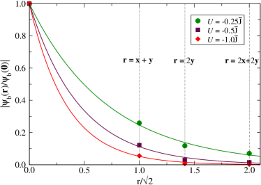
Figure 5: (Color online) Relative amplitude of the wave functions corresponding to three of the bound states shown in Fig. 4, at various distances from the impurity site. Lines are exponential fits. States with bigger binding energies have shorter decay lengths.

Given the almost constant values of $\varepsilon$, $t_{1}$ , $t_{2}$ in this range of energies and the fact that the problem is two dimensional, bound states are expected to appear for any finite $U$. The top panel in Fig. 4 shows the LDOS at the impurity site ${\bf r=0}$ for various values of the on-site attraction $U$. The peaks that appear below the DOS of the clean system (shown by the dashed line) are proportional to Dirac delta functions which are broadened into Lorentzians by the finite $\eta$. They signal the appearance of quasiparticle bound states, characterized by exponential decay of the quasiparticle’s wave function $\psi_{b}({\bf r})$ away from the impurity. The inset verifies that this is true even for the smallest $U$: the height of the ”shoulder”-like feature appearing at the bottom of the band in the main figure scales like $1/\eta$ and evolves into a separate Lorentzian for small enough $\eta$, showing the presence of a bound state below the continuum.

The bottom panel shows the effective attraction at the impurity site $U_{\rm eff}({\bf r=0},\omega)=\mbox{Re}\left[\varepsilon({\bf r=0},\omega)-\varepsilon(\omega)\right]$, i.e. the difference between the effective on-site potential at the impurity site and that at sites far away from the impurity (or in the clean system). Not surprisingly, $U_{\rm eff}({\bf r=0},\omega)\approx U$, although a small dependence of $\omega$ is observed if the scale is significantly expanded.

The exponential decay of the quasiparticle’s wave function can be checked explicitly by calculating the amplitude of these bound states at various distances ${\bf r}$, which is easily done if we note that at $\omega=\omega_{\mathrm{peak}}$ the dominant term in the Lehmann representation is:

$$G_{\bf 0,r}(\omega=\omega_{\mathrm{peak}})\approx{1\over i\eta}\psi_{b}({\bf 0})\psi_{b}({\bf r})^{*}.$$ (21)

Figure 5 shows the ratio $|\psi_{b}({\bf r})/\psi_{b}({\bf 0})|=|G_{\bf 0,r}(\omega=\omega_{\mathrm{peak}})/G_{\bf 0,0}(\omega=\omega_{\mathrm{peak}})|$. The dots are the numerical values, while the lines are exponential fits. Those corresponding to larger binding energies (more negative $\omega_{\mathrm{peak}}$) are more tightly bound to the impurity and therefore decay faster, as expected. This agrees with the larger quasiparticle weight of these states at ${\bf r=0}$, (see Fig. 4). All these results are quite reasonable.

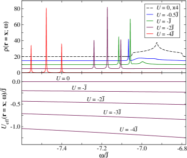
Figure 6: (Color online) (Top) LDOS $\rho({\bf r=x};\omega)$ with curves shifted vertically to help visibility; (Bottom) $U_{\mathrm{eff}}({\bf r=x};\omega)$ at the quasiparticle’s sublattice site located nearest to the impurity. Up to three bound states split from the continuum upon increasing $U$. The presence of the impurity at ${\bf r=0}$ induces a finite effective on-site attraction at ${\bf r=x}$, whose value is significantly smaller than $U$ (Bottom). Parameters are $t=6$, $\mathrm{\bar{J}}=1$, and $\eta=10^{-3}$.

IV.2 Quasiparticle and impurity on different sublattices

We now investigate the more interesting case with the impurity and the quasiparticle located on different sublattices. To this end, we construct the Green’s function $G_{\bf x,R}(\omega)$ in which ${\bf x}$ and ${\bf R}$ are on the quasiparticle’s sublattice [the rotated frame $XY$ is centered to the right of the impurity, see Fig. 2(b)]. In particular, we are interested in the LDOS on this sublattice closest to the impurity $\rho({\bf r=x};\omega)=-\mathrm{Im}G_{\bf x,x}(\omega)/\pi$.

The equations of motion for $G_{\bf x,R}(\omega)$ are derived as before, however now the equations for $F_{1}$ and $F_{3}$ are modified by the presence of the impurity if ${\bf R}$ is close enough to it. This leads to equations of motion for $G_{\bf x,R}(\omega)$ that are similar to those in Eq. (20), but with different values for the effective hoppings and on-site energies close to the impurity. We solve these equations using the same method, but note that now the number of distinct GFs is higher due to the lower symmetry of this case.

In Fig. 6, we plot $\rho({\bf r=x};\omega)$ for various values of $U$. The appearance of Dirac delta peaks shows that bound states exist in this case as well. A comparison with $\rho({\bf r=0};\omega)$ in Fig. 4 for the same value of $U$ shows that these peaks have different energies, therefore they are distinct states. This is further confirmed by the fact that up to three bound states appear here for sufficiently large $U$, as opposed to only one when the quasiparticle and the impurity were on the same sublattice.

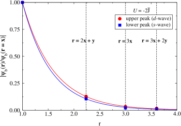
Figure 7: (Color online) Relative amplitude of the upper and lower bound states for $U=-2\mathrm{\bar{J}}$, at various distances from the impurity site. Lines are exponential fits.

These bound states exist in spite of the fact that the impurity is not located on the sublattice in which the quasiparticle propagates. As noted above, within a naive picture one does not expect this: the quasiparticle should not be trapped by an on-site impurity located on the other sublattice. This shows that the quasiparticle does not interact with the bare disorder, but with a renormalized one. This comes about because the quasiparticle’s effective motion on one sublattice is made possible via hopping of the hole through the other sublattice, when the hole and impurity can interact. Indeed, we define the effective on-site attraction:

$$U_{\mathrm{eff}}({\bf x};\omega)=\mathrm{Re}[\varepsilon({\bf x};\omega)-\varepsilon(\omega)|$$

which again compares the effective on-site energy near the impurity to that of sites far away from the impurity (or the clean system). This quantity is plotted in the lower panel of Fig. 6 for various values of $U$. It is finite even though the bare disorder at this site is zero. $U_{\mathrm{eff}}({\bf x};\omega)$ is much weaker than $U$, as expected since it is an indirect effect; this explains why the binding energies for these peaks are much smaller than in the previous case. Retardation effects (dependence on $\omega$) are now clearly visible, especially for the larger $U$ values. They are due to the spin defects accompanying the hole: in order to interact with the impurity, the hole must hop onto its sublattice, however its ability to do so depends on the structure of the surrounding cloud of spin defects. At low energies, the probability for the hole to visit the impurity is further suppressed by the energy cost of the spin defects generated during hopping, explaining why $U_{\mathrm{{eff}}}$ becomes weaker at these energies. A similar effect has been predicted for hole-doped CuO ladders with non-magnetic impurities that affect the propagating holes even if they do not lie in their path.Chudzinski

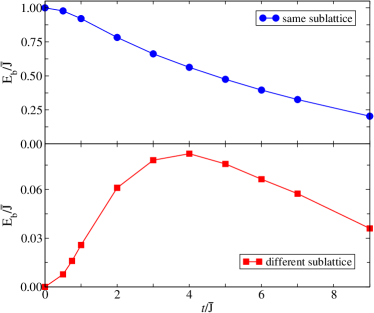
Figure 8: Binding energy of the $s$-wave bound state at $U=-\mathrm{\bar{J}}$ vs. $t/\mathrm{\bar{J}}$, when the quasiparticle and the impurity are on the same sublattice (top panel) and different sublattices (bottom panel). The smaller binding energy at strong hopping is due to the reduction in the quasiparticle’s effective mass, which makes it harder to trap. When the quasiparticle and the impurity are on different sublattices, the enhancement of $U_{\mathrm{{eff}}}$ at small $t$ dominates over the effective mass decrease, explaining the growth of the binding energy here.

Perturbation theory to zero order in $t$ suggests that there should be a finite threshold for $U$ in order for bound states to appear. It can be estimated by comparing the hole’s energy at any other site in the lattice, $4\mathrm{\bar{J}}+{\cal O}(t^{2})$, to its minimum energy at the impurity site, $\mathrm{10\bar{J}}-U+{\cal O}(t^{2})$ (the increased energy is due to the presence of at least one spin defect). If $U<\mathrm{6\bar{J}}$, this implies that it should not be energetically favorable for the hole to be at the impurity site. Including $t^{2}$ corrections does not change this: a finite threshold value is still predicted. However, we do not see any such threshold in the full calculation. This emphasizes again the importance of the (higher-order) loop processes in describing the actual behavior.

As noted, a total of three bound states emerge upon increasing the impurity attraction $U$. Further increase of $U$ increases their binding energy, but it does not give rise to more bound states. One can identify the nature of these bound states by comparing their amplitudes on the four neighboring sites of the impurity, $\langle{\bf r=u}|\psi_{b}\rangle$. These are extracted from $G_{\bf x,u}(\omega=E_{b})$, just as we did in Eq. (21). For the lower peak, we find the same value of $\langle\psi^{1}_{b}|{\bf u}\rangle$ for all ${\bf u}$, implying $s$-wave symmetry. A state with $s$-wave symmetry is expected to have the strongest binding to the impurity since, to the leading order in hopping, all of its four segments meet constructively on the impurity. For the upper peak, $\langle\psi^{3}_{b}\boldsymbol{|}{\bf x}\rangle=-\langle\psi^{3}_{b}\boldsymbol{|}{\bf y}\rangle=\langle\psi^{3}_{b}\boldsymbol{|}{\bf-x}\rangle=-\langle\psi^{3}_{b}\boldsymbol{|}{\bf-y}\rangle$, i.e., this state has $d$-wave symmetry. The middle state has $p_{x}$ symmetry: $\langle\psi^{2}_{b}\boldsymbol{|}{\bf x}\rangle=-\langle\psi^{2}_{b}\boldsymbol{|}{\bf-x}\rangle$ and $\langle\psi^{2}_{b}\boldsymbol{|}{\bf y}\rangle=\langle\psi^{2}_{b}\boldsymbol{|}{\bf-y}\rangle=0$. It has a degenerate twin bound state with $p_{y}$ symmetry, which has zero amplitude at ${\bf r=x}$ and therefore it does not appear in $G_{\bf x,x}(\omega)$. Since the full lattice has rotational symmetry about the impurity, the resulting bound states are expected to mirror this symmetry as well. The spatial profile of $s$- and $d$-wave states is presented in Fig. 7. It shows that they have very similar decay lengths, consistent with their fairly similar binding energies and with the fact that their corresponding peaks in Fig. 6 have similar quasi-particle weights. The $p_{x}$ state, however, is expected to have about twice larger weight as it is divided between only the ${\bf x}$ and ${\bf-x}$ lobes, whereas the $s$ and $d$ states have weights equally distributed in all four directions. Again, this is consistent with its spectral weight shown in Fig. 6.

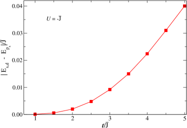
Figure 9: The gap between the $p_{x}$ and either of the $s$ or $d$ states, for a fixed $U$. Its enhancement as a function of $t/\mathrm{\bar{J}}$ reflects the rotational kinetic energy gain of the quasiparticle as it becomes lighter with increasing $t$.

Fig. 8 shows the hole’s binding energy $E_{b}$ for the $s$-states as a function of the hopping $t$, when $U=-\bar{\mathrm{J}}$. It exhibits quite different trends in the two cases. As the hopping becomes stronger, the kinetic energy of the quasiparticle is increased (its effective mass decreases). A lighter quasiparticle is harder to trap and this explains why its binding energy at fixed $U$ gets weaker when it is on the same sublattice with the impurity (top panel).

When the quasiparticle is on the other sublattice (bottom panel) it interacts with the impurity by virtue of $U_{\mathrm{{eff}}}$ which is dynamically generated and therefore strongly depends on $t$. At $t=0$, the hole is locked at a lattice site and is unaware of the presence of impurity, therefore $E_{b}=0$. As $t$ is increased, $U_{\mathrm{{eff}}}$ is enhanced as the hole is able to visit the impurity, whereas the quasiparticle’s effective mass is reduced as it gains more kinetic energy. The former tends to increase the binding energy while the latter reduces it, and it is their competition that sets the dependence of binding energy on hopping. The initial growth of $E_{b}$ implies that the enhancement of $U_{\mathrm{{eff}}}$ dominates over the reduction of effective mass at small $t$. However, since $U_{\mathrm{{eff}}}$ is weaker than $U$ for all $t$ (Fig. 6), further increase of the hopping makes the hole too light to be easily trapped by $U_{\mathrm{{eff}}}$ and the binding energy eventually starts to decrease. While only the binding energy of the $s$-wave state is shown in the lower panel of Fig. 8, all three peaks exist for small $t$, although they are energetically very close to each other. With increasing $t$ they move closer to and eventually merge into the continuum such that, at the highest $t$ considered in Fig. 8, the $s$-wave state is the only existing bound state.

The energy gaps between the three bound states (when all are present) are nearly identical. Figure 9 shows its evolution with $t$ at a fixed value $U=-\bar{\mathrm{J}}$. Since this must be due to differences in the rotational kinetic energy, it is expected to increase with $t$, as the quasiparticle’s effective mass decreases. This is indeed the observed behavior.

V Summary and conclusions

We investigated the effect of a non-magnetic impurity on the motion of a hole in a 2D square Ising AFM. The resulting quasiparticle, which propagates on one sublattice, is confirmed to form bound states around the impurity. This is true both when the hole and impurity are on the same sublattice and when they are on different ones. The latter occurs because of the renormalization of the effective on-site energy which results in finite effective attraction at the sites next to the impurity that can be visited by the quasiparticle. This also explains why a total of (up to) three bound states with $s$, $p$, and $d$ symmetries were found in this case, as opposed to only one $s$-wave state in the case when the quasiparticle is on the same sublattice with the impurity. In this latter case, the impurity is located in the node of $p$ and $d$ symmetry states, therefore such states do not see it and can not be bound to it. (In reality, a non-zero $U_{\rm eff}$ arises at sites different from those occupied by the impurity, but given the longer distance to the impurity site, this is not large enough to bind new states).

Bound states with $s$, $p$, and $d$ symmetries have also been observed near an inert vacancy in a Heisenberg AFM. However, in that case, it is the distortion of the magnetic environment around the vacancy that binds the hole.Poilblanc1 ; Poilblanc2 Such a distortion is only possible in a Heisenberg model and comes from a local modification of the spin fluctuations. In an Ising AFM, an inert site would have no effect on the AFM order of the other sites. Moreover, if the hole is not allowed to visit this inert impurity site, there are no Trugman loops including it so the hole loses kinetic energy when located in that neighborhood. As a result, we expect that in an Ising AFM, an inert impurity like that of Ref. Poilblanc1, would repulse the hole. Bound states could only appear if a sufficiently strong exchange was turned on between the hole and the inert spin, so that the exchange energy gained through it compensated for the loss of kinetic energy. Such a model was analyzed in Ref. Poilblanc2, , although for the Heisenberg model it was found that bound states persist only if this exchange with the inert site is rather weak. All these differences show that the underlying reasons for the appearance of bound states are very different in these other models. This is further substantiated by the fact that while a sublattice dependence is observed in Refs. Poilblanc1, ; Poilblanc2, , it consists of a variation of the spectral weight but this is associated with the same eigenstates. By contrast, in our model, the two sublattices show different spectra of bound states.

This result is important because it suggests that two very different patterns of bound states should be observed with scanning tunneling microscopy (STM) in such systems, even if only one type of impurity is present. Note that we assumed that the impurity is located directly at (or above) a lattice site. If, on the other hand, the impurity was located either half-way between two sites or in the center of the plaquettes, then it would not break the symmetry between the two sublattices and only one pattern of bound states should appear. These cases can be studied by similar means as presented here.

A major simplifying factor of this problem was the assumption of an Ising AFM. If spin fluctuations are turned on, in a Heisenberg AFM, a major difference is that the hole no longer needs to go twice around closed loops in order to become delocalized: spin fluctuations can remove pairs of neighboring spin defects, thus cutting the string short and releasing the hole. As a result, one expects a significant decrease in the effective mass of the quasiparticle, which is indeed observed.Trugman However, it is interesting to note that if there is true long-range AFM order in the plane (as is the case in cuprates, due to coupling between planes), the resulting quasiparticle should continue to primarily reside on one sublattice, because spin fluctuations can only remove pairs of spin defects and spin conservation would continue to make the two sublattices inequivalent. This suggests that the results we present here, which are directly traceable to the fact that the quasiparticle lives on one sublattice, could be relevant for the Heisenberg AFM as well, although it is impossible to say a priori if the effective attraction generated when the quasiparticle and impurity are on different lattices would suffice to bind states (we would still expect $s$-symmetry bound states to appear if the quasiparticle and impurity are on the same sublattice). A follow-up of this issue would be interesting.

In the broader context, these results confirm the view that coupling to bosonic degrees of freedom renormalizes not just a quasiparticle’s dispersion, but also the effective disorder it sees. If the latter were not the case, no bound states could arise when the quasiparticle lives on a difference sublattice than the impurity. Similar large and non-trivial renormalization of the disorder seen by a dressed quasiparticle, arising from its coupling to bosons, was also demonstrated for lattice polarons.earlier

Appendix A The equations of motion for $G_{\bf 0,R}(\omega)$

Here we present the details of the calculations that lead to Eq. (10), which relates the various $G_{\bf 0,R}(\omega)$ GFs. Eq. (9) enables us to eliminate $F_{3}$ from Eq. (8) to obtain:

$$F_{2}({\bf R},{\bf u},{\bf v})-t^{2}\bar{g}_{2}g_{3}F_{2}({\bf R+u+v,-v,-u})\\ =-t\bar{g}_{2}F_{1}({\bf R,u}),$$ (22)

and

$$F_{2}({\bf R+u+v},{\bf-v},{\bf-u})-t^{2}\bar{g}_{2}g_{3}F_{2}({\bf R,u,v})\\ =-t\bar{g}_{2}F_{1}({\bf R+u+v,-v}),$$ (23)

where $\bar{g}_{2}=1/(\omega-14\mathrm{\bar{J}}-t^{2}g_{3}+i\eta)$ and Eq. (23) results from Eq. (22) after changing the coordinates ${\bf R\rightarrow R+u+v}$, ${\bf u\rightarrow-v}$, ${\bf v\rightarrow-u}$. Solving the coupled equations (22) and (23), we find

$$F_{2}({\bf R},{\bf u},{\bf v})=\gamma_{1}F_{1}({\bf R},{\bf u})+\gamma_{2}F_{1}({\bf R+u+v},{\bf-v}),$$ (24)

in which $\gamma_{1}=-t\bar{g}_{2}/[1-(t^{2}\bar{g}_{2}g_{3})^{2}]$ and $\gamma_{2}=t^{2}\bar{g}_{2}g_{3}\gamma_{1}$. Using this in Eq. (7) gives

$$F_{1}({\bf R},{\bf u})=\\ -t\bar{g}_{1}[G_{\bf 0,R}+\gamma_{2}\sum_{\bf v\perp u}F_{1}({\bf R+u+v},{\bf-v})],$$ (25)

in which $\bar{g}_{1}=1/(\omega-10\mathrm{\bar{J}}+2t\gamma_{1}+i\eta)$ and the sum includes the two nearest-neighbor vectors, ${\pm\bf v}$, along the direction perpendicular to ${\bf u}$. With a proper change of coordinates, each $F_{1}$ on the right-hand side of Eq. (25) can be expressed in term of a component of $G$ and new $F_{1}$’s. For example,

$$F_{1}({\bf R+u+v},{\bf-v})+t\bar{g}_{1}G_{\bf 0,R+u+v}=\\ -t\bar{g}_{1}\gamma_{2}[F_{1}({\bf R+2u,-u})+F_{1}({\bf R,u})],$$ (26)

and

$$F_{1}({\bf R+u-v},{\bf v})+t\bar{g}_{1}G_{\bf 0,R+u-v}=\\ -t\bar{g}_{1}\gamma_{2}[F_{1}({\bf R+2u,-u})+F_{1}({\bf R,u})],$$ (27)

which results after applying either of ${\bf R\rightarrow R+u\pm v}$, ${\bf u\rightarrow\mp v}$, ${\bf v\rightarrow u}$ to Eq. (25), respectively. The additionally introduced $F_{1}$ can be written in terms of the existing ones by doing ${\bf R\rightarrow R+2u}$, ${\bf u\rightarrow-u}$ on Eq. (25)

$$F_{1}({\bf R+2u,-u})+t\bar{g}_{1}G_{\bf 0,R+2u}=\\ -t\bar{g}_{1}\gamma_{2}[F_{1}({\bf R+u+v,-v})+F_{1}({\bf R+u-v,v})].$$ (28)

The four equations (25) to (28) can be simultaneously solved for the four $F_{1}$’s in terms of the existing components of $G$. In particular, we find:

$$F_{1}({\bf R,u})=\zeta_{1}G_{\bf 0,R}\\ +\zeta_{2}G_{\bf 0,R+2u}+\zeta_{3}[G_{\bf R+u+v}+G_{\bf R+u-v}],$$ (29)

where $\zeta_{1}=-t\bar{g}_{1}[1-2(t\bar{g}_{1}\gamma_{2})^{2}]/[1-4(t\bar{g}_{1}\gamma_{2})^{2}]$, $\zeta_{2}=-2t\bar{g}_{1}(t\bar{g}_{1}\gamma_{2})^{2}/[1-4(t\bar{g}_{1}\gamma_{2})^{2}]$ and $\zeta_{3}=-t\bar{g}_{1}\gamma_{2}(\zeta_{1}+\zeta_{2})$. Finally, using this in Eq. (6) results in the equation of motion for the GF

$$G_{\bf 0,R}(\omega)=\bar{g}_{0}(\omega)[\delta_{\bf R,0}\\ -t_{1}(\omega)\sum_{{\bf\boldsymbol{\delta}}}G_{\bf 0,R+{\boldsymbol{\delta}}}(\omega)-t_{2}(\omega)\sum_{{\boldsymbol{\xi}}}G_{\bf 0,R+\boldsymbol{\xi}}(\omega)],$$ (30)

and its various coefficients are given in the text following Eq. (10).

These effective hoppings and on-site energies are identical to those derived for the clean system in Ref. Mona, .typo In the presence of disorder, the solution proceeds similarly but now the various $g$ functions acquire dependence on the location since their argument is shifted by $U$ if ${\bf R=0}$. This leads to dependence on location (and even direction of hopping) for the effective hopping and on-site energies, at sites close enough to the impurity.

References

- (1) C. L. Kane, P. A. Lee, and N. Read, Phys. Rev. B 39, 6880 (1989).
- (2) F. Marsiglio, A. E. Ruckenstein, S. Schmitt-Rink, and C. M. Varma, Phys. Rev. B 43, 10882 (1991).
- (3) S. Sachdev, Phys. Rev. B 39, 12232 (1989).
- (4) A. V. Chubukov and D. K. Morr, Phys. Rev. B 57, 5298 (1998).
- (5) B. I. Shraiman and E. D. Siggia, Phys. Rev. Lett. 60, 740 (1988).
- (6) P. A. Lee, N. Nagaosa, and X. G. Wen, Rev. Mod. Phys. 78, 17 (2006).
- (7) P. Phillips, Rev. Mod. Phys. 82, 1719 (2010).
- (8) E. Dagotto, R. Joynt, A. Moreo, S. Bacci and E. Gagliano, Phys. Rev. B 41, 9049 (1990); H. Fehske, V. Waas, H. Röder and H. Büttner, ibid. 44, 8473 (1991); E. Dagotto, Rev. Mod. Phys. 66, 763 (1994).
- (9) J. Riera, S. Koval, D. Poilblanc, and F. Pantigny, Phys. Rev. B. 54, 7441 (1996); G. Xiao, M. Z. Cieplak, J. Q. Xiao, and C. L. Chien, Phys. Rev. B 42, 8752 (1990).
- (10) D. N. Basov, B. Dabrowski, and T. Timusk, Phys. Rev. Lett. 81, 2132 (1998).
- (11) H. Alloul, J. Bobroff, M. Gabay, and P. J. Hirschfeld, Rev. Mod. Phys. 81, 45 (2009).
- (12) D. Heidarian and N. Trivedi , Phys. Rev. Lett. 93, 126401 (2004); Yun Song, R. Wortis and W. A. Atkinson, R. Wortis and W. A. Atkinson, Phys. Rev. B 77, 054202 (2008); Phys. Rev. B 82, 073107 (2010).
- (13) A. Suchaneck, V. Hinkov, D. Haug, L. Schulz, C. Bernhard, A. Ivanov, K. Hradil, C. T. Lin, P. Bourges, B. Keimer, and Y. Sidis, Phys. Rev. Lett. 105, 037207 (2010).
- (14) S. Wessel, B. Normand, M. Sigrist, and S. Haas, Phys. Rev. Lett. 86, 1086 (2001).
- (15) D. Poilblanc, D.J. Scalapino, and W. Hanke, Phys. Rev. Lett. 72, 884 (1994).
- (16) D. Poilblanc, D.J. Scalapino, and W. Hanke, Phys. Rev. B. 50, 13020 (1994).
- (17) W. F. Brinkman and T. M. Rice, Phys. Rev. B 2, 1324 (1970).
- (18) D. Poilblanc, H. J. Schulz, and H. T. Ziman, Phys. Rev. B 47, 3268 (1993).
- (19) S. A. Trugman, Phys. Rev. B 37, 1597 (1988).
- (20) M. Berciu and and H. Fehske, Phys. Rev. B 84, 165104 (2011). If the constraints are not enforced, this model is known as the Edwards model and has been shown to have interesting behavior, for example see: A. Alvermann, D. M. Edwards and H. Fehske, Phys. Rev. Lett. 98, 056602 (2007); S. Ejima, G. Hager and H. Fehske, Phys. Rev. Lett. 102, 106404 (2009).
- (21) Note that Eq. (18) in Ref. Mona, has a typo in the denominator, where the prefactor 4 behind has to be replaced with 2.
- (22) J. Riera and E. Dagotto, Phys. Rev. B 47, 15346 (1993); E. Lahoud, O. Nganba Meetei, K. B. Chaska, A. Kanigel, and N. Trivedi, arXiv:1303.0649v1.
- (23) M. Möller, A. Mukherjee, C. P. J. Adolphs, D. J. J. Marchand, and M. Berciu, J. Phys. A: Math. Theor. 45, 115206 (2012).
- (24) P. Chudzinski, M. Gabay, and T. Giamarchi, New J. Phys. 11, 055059 (2009).
- (25) M. Berciu, A. S. Mishchenko, and N. Nagaosa, Europhys. Lett. 89, 37007 (2010); H. Ebrahimnejad and M. Berciu, Phys. Rev. B 85, 165117 (2012); H. Ebrahimnejad and M. Berciu, Phys. Rev. B 86, 205109 (2012).