The ‘Higgs’ amplitude mode in weak ferromagnetic metals

Abstract

Using Ferromagnetic Fermi liquid theory, Bedell and Blagoev derived the collective low-energy excitations of a weak ferromagnet. They obtained the well-known magnon (Nambu-Goldstone) mode and found a new gapped mode that was never studied in weak ferromagnetic metals. In this article we have identified this mode as the Higgs boson (amplitude mode) of a ferromagnetic metal. This is identified as the Higgs since it can be show that it corresponds to a fluctuation of the amplitude of the order parameter. We use this model to describe the itinerant-electron ferromagnetic material MnSi. By fitting the model with the existing experimental results, we calculate the dynamical structure function and see well-defined peaks contributed from the magnon and the Higgs. Our estimates of the relative intensity of the Higgs amplitude mode suggest that it can be seen in neutron scattering experiments on MnSi.

The emergence of low-energy excitations in systems with spontaneously broken symmetry plays a very important role in our fundamental understanding of nature. There are two types of fundamental excitations (particles) that may be present in the field theory descriptions of these spontaneously broken symmetries: massless Nambu-Goldstone bosons (magnons, or phase modes) and massive Higgs bosons (amplitude modes). Let the order parameter that describes a state with a spontaneously broken symmetry be $\phi({\bf x})=\rho({\bf x})e^{i\theta({\bf x})}$. Then, in the ground state we have $<\phi({\bf x})>=\rho_{0}e^{i\theta_{0}}$, where finite values for $\theta_{0}$ and $\rho_{0}$ correspond to a broken symmetry. The two fundamental excitations are the Nambu-Goldstone boson, which corresponds to fluctuations of the phase of the order parameter with fixed amplitude, $\rho_{0}$, and the Higgs boson, with fluctuations of $\rho({\bf x})$ with the phase fixed at $\theta_{0}$.

The understanding of the amplitude mode is particularly important for the Standard model of elementary particle physicsW . Recent experiments from LHCLHC1 ; LHC2 which detected Higgs-like particles has drawn much attention to this subject. This Higgs-like mode was predicted theoretically and found experimentally in many condensed matter systems. This includes incommensurate charge-density-wave (CDW) statesLRA , superconducting systemsSK ; LV1 ; LV2 ; V , and lattice Boson systems with superfluid and Mott insulator transitionPAP ; AA ; PP ; HABB ; Nature , which can be realized by ultracold bosonic atoms on an optical lattice.

In this article we have identified the amplitude mode in another well-known system with spontaneously broken symmetry, a ferromagnetic metal. The Nambu-Goldstone magnon mode in ferromagnetic systems was first predicted by BlochB and SlaterS , and observed in iron in a neutron scattering experimentL . Abrikosov and DzyaloshinkiiAD first predicted spin waves in ferromagnetic Fermi liquids using a ferromagnetic Fermi liquid theory (FFLT) for itinerant ferromagnets. This approach was put on a more microscopic foundation in the work of Dzyaloshinskii and KondratenkoDK . Moriya and Kawabata also developed a band theory (MK theory) to study the long wavelength spin fluctuation in itinerant ferromagnetic systemsMK . Bedell and BlagoevBB generalized the FFLT and they discovered a new collective mode of the system; they found a mode with a gap in the excitation spectrum. We have identified this mode as the Higgs amplitude mode of a ferromagnetic metal.

We begin by quickly describing the FFLT approach used by Bedell and Blagoev BB , in the small magnetic moment limit, to study the collective excitations in a ferromagnetic metal. We then arguee that the massive mode is indeed an amplitude mode. To estimate the collective modes’ frequencies we use a simple one-band description with a spherical Fermi surface for the itinerant-electron ferromagnet MnSi. By fitting existing experimental results we can pin down some of the Landau parameters and use them to calculate dynamical structure function, $S(q,\omega)$. As we will see there are two sharp peaks in $S(q,\omega)$ corresponding to the two collective modes, the well-known Nambu-Goldstone mode (sometimes referred to as the transverse spin wave) and a gapped Higgs amplitude mode. From our estimates of the spectral weight of the amplitude mode it should be observable in neutron scattering experiments.

We consider a three dimensional weak ferromagnetic material below its Curie temperature. According to FFLT, in the weak moment limit, the system can be described by the quasi-particle distribution function $n_{{\bf p}\alpha\alpha^{{}^{\prime}}}(\vec{r},t)=n_{\bf p}({\bf r},t)\delta_{\alpha\alpha^{{}^{\prime}}}+{\bf m_{p}}({\bf r},t)\cdot\vec{\sigma}_{\alpha\alpha^{{}^{\prime}}}$, and the quasi-particle energy function $\epsilon_{{\bf p}\alpha\alpha^{{}^{\prime}}}(\vec{r},t)=\epsilon_{\bf p}({\bf r},t)\delta_{\alpha\alpha^{{}^{\prime}}}+{\bf h_{p}}({\bf r},t)\cdot\vec{\sigma}_{\alpha\alpha^{{}^{\prime}}}$BP ; AD , with ${\bf m_{p}}$ the quasi-particle magnetization and ${\bf h_{p}}=-{\bf B}+2\sum_{\bf p^{\prime}}f_{\bf pp^{\prime}}^{a}{\bf m_{p}^{\prime}}$ the effective magnetic field which includes the external magnetic field $\bf B$ and the internal magnetic field generated by quasi-particle interactions $f_{\bf pp^{{}^{\prime}}}^{a}$. Here and throughout the paper we set $\mu_{mag}=\frac{\gamma\hbar}{2}=1$ and $\hbar=1$. The quasi-particle interaction can be expanded in Legendre Polynomials, and in this weak moment limit, it can be treated as spin rotation invariantBEB , so that it can be separated into the spin symmetric and spin anti-symmetric parts $N(0)f_{\bf pp^{\prime}}^{\sigma\sigma^{\prime}}=\sum_{l}(F_{l}^{s}+F_{l}^{a}\sigma\cdot\sigma^{\prime})P_{l}(\hat{\bf p}\cdot\hat{\bf p}^{\prime}).$ Here, $N(0)$ is the average density of states over the two Fermi surfaces and in the ferromagnetic phase, $F_{0}^{a}<-1$. This state can be said to be protected by the generalized Pomeranchuck stability conditionP ; YB , and its ground state is described by the distribution function ${\bf m}_{\bf p}^{0}=-{\bf m}_{0}\partial n_{{\bf p}}^{0}/\partial\varepsilon_{{\bf p}}^{0},$ where ${\bf m}_{0}$ is the equilibrium magnetization divided by $N(0)$. Fluctuations about equilibrium, $\delta{\bf m_{p}}$, are described by a linearized spin kinetic equation,BP

$$\frac{\partial{\delta\bf m_{p}}({\bf r},t)}{\partial t}+{\bf v_{p}}\cdot{\bf\nabla}(\delta{\bf m_{p}}({\bf r},t)-\frac{\partial n_{\bf p}^{0}}{\partial\varepsilon_{\bf p}^{0}}\delta{\bf h_{p}}({\bf r},t))\\ =-2({\bf m}_{\bf p}^{0}({\bf r},t)\times\delta{\bf h}_{\bf p}({\bf r},t)+\delta{\bf m_{p}}({\bf r},t)\times{\bf h}_{\bf p}^{0}({\bf r},t))+I[{\bf m_{p}}]$$ (1)

where ${\bf h_{p}^{0}}=-{\bf B}+2\sum_{\bf p^{\prime}}f_{\bf pp^{\prime}}^{a}{\bf m_{p}^{\prime}}$ and $\delta{\bf h_{p}}=-\delta{\bf B}+2\sum_{\bf p^{\prime}}f_{\bf pp^{\prime}}^{a}\delta{\bf m_{p}^{\prime}}$ are the effective equilibrium field and its fluctuation, respectively. Here, a small magnetic field $\delta{\bf B}$ is set transverse to the equilibrium magnetization. A direct way to obtain the dispersions is to take the limit of free oscillations of Eq.(1) by setting ${\bf B}=0$ and ${\delta\bf B}=0$, and looking at the low temperature limit for which the collision integral $I[{\bf m_{p}}]$ can be ignored. This is the quantum spin hydrodynamic regime whose details of the derivation are more explicit in Ref.BB, . In addition to the free oscillation limit, it is also possible to use Eq.(1) to calculate the response function $\chi(q,\omega)$ that relates ${\delta\bf B}$ with its induced transverse response $\delta{\bf m}=\sum_{\bf p}\delta{\bf m_{p}}$ ($\delta{\bf m}=\chi(q,\omega)\delta{\bf B}$) and from it the dynamical structure function $S(q,\omega)=-Im[\chi(q,\omega)]/\pi$. The calculations are done by projecting out the $l$ components of both the kinetic equation and the spin density distribution function $\delta{\bf m_{p}}=-(\partial n_{\bf p}^{0}/\partial\varepsilon_{\bf p}^{0})\sum_{l}{\bm{\nu}}_{l}P_{l}(\hat{\bf p}\cdot\hat{z})$. We will return to the full calculation of $S(q,\omega)$ a little later.

We can use the kinetic equation to derive the continuity equation for the magnetization and the equation of the spin current defined as ${\bf j}_{i}^{\sigma}({\bf r},t)=\sum_{\bf p}v_{pi}{\bf m_{p}}({\bf r},t)(1+F_{1}^{a}/3)$. The dispersions found using the free- oscillation limit are

$$\omega_{1}^{\pm}(q)=\frac{c_{s}^{2}}{\omega^{\pm}}q^{2},$$ (2)

$$\omega_{2}^{\pm}(q)=\omega^{\pm}-\frac{c_{s}^{2}}{\omega^{\pm}}q^{2}$$ (3)

where $\omega^{\pm}=\pm 2m_{0}\left|F_{0}^{a}-F_{1}^{a}/3\right|$, $c_{s}^{2}=\left|1+F_{0}^{a}\right|(1+F_{1}^{a}/3)v_{F}^{2}/3$, and $v_{F}$ is the Fermi velocity on the average Fermi surface. The $\pm$ signs correspond simply to the different precessional directions so that we effectivelly have two modes.

Before we go to the full calculation of $S(q,\omega)$, we can extract the basic physics from these results. The ‘Standard Model’ of a ferromagnetic metal is often referred to as the Stoner model and it can best be characterized by its elementary excitations. To begin with there are the spin 1/2 particle-like excitations (sometimes referred to as quasi-particles), consisting of up spins ($\sigma=\uparrow$ ), majority spins, and down spins ($\sigma=\downarrow$ ), minority spins. In the presence of spontaneous long range ferromagnetic order there are also gapless transverse spin waves (the Nambu-Goldstone mode). This mode has a total spin of $\pm 1$ associated with the two precessional directions of the equilibrium magnetization. For simplicity, in what follows we will consider only the spin $+1$ excitations. If we think in terms of the order parameter for the ferromagnetic state this would be a fluctuation of the phase (rotation about the z axis in space) with the magnitude of the order parameter fixed at its equilibrium value, $m_{0}$. In addition to these spin waves, there are other spin $+1$ excitations in the Stoner model that correspond to fluctuations in the magnitude of the order parameter at a fixed phase. At $q=0$ these excitations have a gap in their spectrum usually referred to as the Stoner gap. For $q\neq 0$, these spin $+1$ excitations have a range of frequencies (shaded region shown in Fig.1) and these are the incoherent particle-hole excitations, $\omega_{p-h}^{\pm}=\mp 2m_{0}F_{0}^{a}+{\bf q}\cdot{\bf v_{p}}$. These excitations are not collective, thus, there is no Higgs amplitude mode in the Stoner model: When the momentum-transfer, $q$, is large enough the Goldstone mode decays into these incoherent particle-hole excitations (Landau damping), while the gapped exitations are Landau damped for all values of $q$.

The FFLT description of Bedell and Blagoev[20] for small momentum transfers is qualitatively the same as the Stoner model if we set all Landau parameters, $F_{l}^{a}=0$, for all $l>0$, and keep only $F_{0}^{a}$. If we keep only the $l=0$ and $l=1$ moments of the spin density distribution function ($\nu_{0}$ and $\nu_{1}$), we get the two modes, Eqs.(2) and (3). The first mode is just the Nambu-Goldstone mode and the second mode has a gap in its spectrum, where at $q=0$, it is just the Stoner gap, $\omega_{2}^{+}=2\left|F_{0}^{a}\right|m_{0}$. This excitation causes a change in the magnitude (amplitude) of the order parameter since it is a spin flip process. In the spin flip process we take a down spin and flip it to an up spin causing an amplitude fluctuation since we decreased the number of down spins while increasing the number of up spins during this fluctuation. These fluctuations of the amplitude of the order parameter could have been the Higgs amplitude mode, however, in the Stoner model this mode sits in the particle-hole continuum and it is Landau damped; it is not a collective mode.

The Fermi liquid description of the collective modes of a Ferromagnetic metalBB goes beyond the Stoner model described above in a simple but most important way. As can be seen from Eqs.(2) and (3) there are two modes, the first one is the Goldstone mode. The second mode has a gap in its spectrum given by $\omega_{2}^{+}=2m_{0}\left|F_{0}^{a}-F_{1}^{a}/3\right|$. The introduction of the higher order Fermi liquid parameter $F_{1}^{a}$ is responsible for the propagation of the mode. This parameter couples the momentum of the quasi-particle to its spin and it is responsible for pushing the mode out of the particle-hole continuum. Most of the spectral weight in this propagating mode comes from the incoherent particle-hole continuum. As we noted earlier the particle-hole continuum is made up from incoherent spin flip (spin $+1$) excitations and they correspond to an amplitude fluctuation. This mode can sit above the Stoner gap for positive $F_{1}^{a}$ and below the Stoner gap for negative $F_{1}^{a}$, with the lower bound, $F_{1}^{a}>-3$YB . It propagates and is built out of fluctuations that change the amplitude of the order parameter, thus it is the ferromagnetic metal example of the Higgs amplitude mode. Also since it couples to the spin fluctuations it can be seen in the transverse spin fluctuation response function that could be measured in a neutron scattering experiment, as we see below.

We calculate the dynamical spin-spin response function based on the kinetic equation, Eq.(1). Here we go beyond the hydrodynamic approach by keeping ${\bm{\nu}}_{l}$ for arbitrary values of $l$ and the Landau parameters $F_{l}^{a}$ up to $l=1$. The response function obtained is given by

$$\frac{\chi(q,\omega)}{N(0)}=\frac{-\chi_{0}^{+}+\frac{2m_{0}F_{1}^{a}}{qv_{F}(1+F_{1}^{a}/3)}\chi_{1}^{+}}{1-F_{0}^{a}\chi_{0}^{+}-\frac{\omega}{qv_{F}}\frac{F_{1}^{a}}{1+F_{1}^{a}/3}\chi_{1}^{+}}$$ (4)

where

$$\begin{split}&\chi_{0}^{+}(q,\omega)=-1\\ &\ +\frac{1}{2qv_{F}}[\omega+2m_{0}(1+F_{0}^{a})]\ln{\left(\frac{\omega+2m_{0}F_{0}^{a}+qv_{F}}{\omega+2m_{0}F_{0}^{a}-qv_{F}}\right)},\end{split}$$ (5)

$$\begin{split}&\chi_{1}^{+}(q,\omega)=-\frac{1}{qv_{F}}[\omega+2m_{0}(1+F_{0}^{a})]\\ &\times[1-\frac{1}{2qv_{F}}(\omega+2m_{0}F_{0}^{a})\ln\left(\frac{\omega+2m_{0}F_{0}^{a}+qv_{F}}{\omega+2m_{0}F_{0}^{a}-qv_{F}}\right)].\end{split}$$ (6)

From the response function, we obtain the dynamic structure function $S(q,\omega)=-Im[\chi(q,\omega)]/\pi$, whose poles will give, for small $q$s, $\omega_{1}^{+}(q)$ and $\bar{\omega}_{2}^{+}(q)=\omega^{+}-(\frac{c_{s}^{2}}{\omega^{+}}-\alpha)q^{2}$ with $\alpha=2v_{F}^{2}(1+3/F_{1}^{a})/15m_{0}$, corresponding to the two collective modes derived in hydrodynamic approach respectively. In [20] it was noted that ${\bm{\nu}}_{2}$ is of the same order of ${\bm{\nu}}_{1}$ while ${\bm{\nu}}_{l}\ll{\bm{\nu}}_{2}$ for all $l\geq 3$. In our calculation we look for the pole of the response function, which includes all ${\bm{\nu}}_{l}$s. A comparison to the modes obtained in Ref.BB, with the hydrodynamic approach is illustrated in Fig.(1).

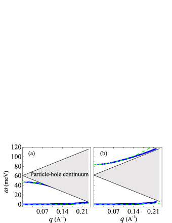
Figure 1: (color on line) Collective modes together with the p-h continuum in the case (a) $F_{0}^{a}=-1.18$, $F_{1}^{a}=-0.84$ and (b) $F_{0}^{a}=-1.16$, $F_{1}^{a}=1.32$. The green-dashed lines represent the dispersion calculated using the hydrodynamic approach, Eqs.(2) and (3) while the blue-solid lines are the dispersions taken from the poles of the response function. Plots obtained by using parameters fitted to early experiments (see text), including the following: $N(0)=6.4\times 10^{29}\;{\rm eV^{-1}m^{-3}}$, $k_{F}=1.23\;{\rm\AA}^{-1}$, $m^{*}=39.3m_{e}$, $E_{F}=0.147\;{\rm eV}$, and $v_{F}=3.63\times 10^{4}\;{\rm ms^{-1}}$.

It shows, as expected, agreement of the two results over a considerable range of small values for $q$. However, the full calculation of $S(q,\omega)$ captures additional features, as, e.g., seen in Fig.(2) where the value of $F_{1}^{a}$ is varied to illustrate the building of the Higgs mode out of the particle-hole continuum. As we noted earlier, all of the spectral strength for the Higgs mode comes from the continuum, which makes the observation of the continuum itself difficult, as it is known from neutron scattering experiments.

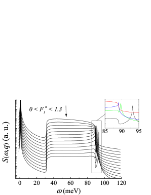
Figure 2: (color on line) Dynamic structure function for different values of of $F_{1}^{a}$. As $F_{1}^{a}$ is switched on, the Higgs builds out of the particle-hole continuum (the wider peak in the middle) while the Goldstone mode remains approximately unchanged.

The itinerant ferromagnetic material MnSi is a very good candidate for the experimental search of the Higgs mode. MnSi is metallic and it behaves ferromagnetically in a magnetic fieldWWSW ; SA ; WWS ; LLS . Neutron scattering leads to the magnon dispersionIST , $\omega\;({\rm meV})=0.13+52q^{2}\;({\rm\AA^{-2}})$ and specific heat measurement givesCV1 ; CV2 $(C/T)_{0}=85*10^{-}4\;{\rm cal/(K^{2}mole})$. From the band structure calculationJP , we know the density of the quasi-particles. We fit the experimental data to a single band description with the quadratic dispersion $E=\hbar^{2}k^{2}/2m^{*}$, which keeps the volume of the Fermi surface unchanged. We obtain all the parameters we need and a relationship between two of the Landau parameters, $F_{1}^{a}=-(375+321F_{0}^{a})/(143+125F_{0}^{a})$. Since the system is weakly ferromagnetic, $F_{0}^{a}$ should be close to and smaller than $-1$, and $F_{1}^{a}$ depends on $F_{0}^{a}$ very sensitively in this region. We don’t have extra experimental results to pin down the sign of $F_{1}^{a}$, so we take the values of ($F_{0}^{a}$, $F_{1}^{a}$) to be (-1.16, 1.32) and (-1.18,-0.84) as typical examples to show the two collective modes in these two cases.

Figure 3: Dynamical structure function showing both the collective modes and the p-h continuum in the cases of $F_{0}^{a}=-1.16,$ $F_{1}^{a}=1.32$ (a) and $F_{0}^{a}=-1.18$, $F_{1}^{a}=-0.84$ (b).

Fig.(3) shows the dynamic structure function in the two typical cases for different momentum transfer. We can clearly see the two sharp peaks contributed by the two collective modes and the wider one coming from the p-h continuum.

In summary, following from the earlier work of Bedell and BlagoevBB , we used the ferromagnetic Fermi liquid theory to study the collective modes in a weak ferromagnetic metal. In addition to the well-known magnon (the phase mode), a gapped mode was also foundBB . We have shown here that this gapped mode corresponds to the Higgs amplitude mode. This mode sits close to the Stoner gap and is propagating at small $\bf q$ and becomes Landau damped at larger $\bf q$. We believe that this is the first time that the Higgs amplitude mode has been predicted in a weak ferromagnetic metal. We believe the itinerant weak ferromagnet MnSi is a good candidate to search for this mode and that it should be visible in inelastic neutron scattering experiments.

We would like to thank Stephen Wilson and Krastan Blagoev for valuable discussion and advice.

References

- (1) S. Weinberg, The Quantum Theory of Fields Vol.2, (Cambridge Univ. Press, 1991).
- (2) ATLAS Collaboration, Phys. Lett. B 716 1 C29 (2012).
- (3) CMS Collaboration, Phys. Lett. B 716 30-61 (2012).
- (4) P.A. Lee, T.M. Rice and P.W. Anderson, Solid State Commun. 14, 703 (1974).
- (5) R. Sooryakumar and M.V. Klein, Phys. Rev. Lett. 45, 660 (1980).
- (6) P.B. Littlewood and C.M. Varma, Phys. Rev. Lett. 47, 811 (1981).
- (7) P.B. Littlewood and C.M. Varma, Phys. Rev. B 26, 4883 (1982).
- (8) C.M. Varma, J. Low Temp. Phys. 126, 901 (2002).
- (9) D. Podolsky, A. Auerbach and D.P. Arovas, Phys. Rev. B 84, 174522 (2011).
- (10) E. Altman and A. Auerbach, Phys. Rev. Lett. 89, 250404 (2002).
- (11) L. Pollet and N. Prokof’ev, Phys. Rev. Lett. 109, 010401 (2012).
- (12) S.D. Huber, E. Altman, H.P. Büchler and G. Blatter, Phys. Rev. B 75, 085106 (2007).
- (13) M. Endres, T. Fukuhara, D. Pekker, M. Cheneau, P. Schaub, C. Gross, E. Demler, S. Kuhr, and I. Bloch, Nature 487, 454 (2012).
- (14) F. Bloch, Z. Phys. 31, 206 (1930).
- (15) J.C. Slater, Phys. Rev. 35, 509 (1930).
- (16) R.D. Lowde, Proc. R. Soc. A, 235, 305 (1956).
- (17) A.A. Abrikosov and I.E. Dzyaloshinskii, Sov. Phys. JETP 35, 535 (1959).
- (18) I.E. Dzyaloshinskii and P.S. Kondratenko, Zh. Eksp. Teor. Fiz. 70, 1987-2005 (1976).
- (19) T. Moriya and A. Kawabata, J. Phys. Soc. Jpn. 34, 639 (1973); see also, T. Moriya, Physica (Utr.) 8 91, 235 (1977).
- (20) K.S. Bedell and K.B. Blagoev, Philos. Mag. Lett. 81, 511 (2001).
- (21) G. Baym and C. Pethick, Landau Fermi-liquid Theory, (John Wiley & Sons. Inc., 1991).
- (22) K.B. Blagoev, J. R. Engelbrecht, and K.S. Bedell, Phys. Rev. Lett. 82, 133 (1999); K.B. Blagoev, J. R. Engelbrecht, and K.S. Bedell, Philos. Mag. Lett. 78, 169 (1998).
- (23) I.I. Pomeranchuk, Sov. Phys. JETP 8, 361 (1959).
- (24) Yi Zhang and K.S. Bedell, Phys. Rev. B 87 115134(2013).
- (25) H.J. Williams, J.H. Wernick, R.C. Sherwood, and G.K. Wertheim, J. Appl. Phys. 37, 1256 (1966).
- (26) D. Shinoda and S. Asanabe, J. Phys. Soc. Jpn. 21, 555 (1966).
- (27) J.H. Wernick, G.K. Wertheim, and R.C. Sherwood, Mat. Res. Bull. 7, 1431 (1971).
- (28) L.M. Levinson, G.H. Lander, and M.O. SteInitz, AIPConf. Proc. 10, 1138 (1972).
- (29) Y. Ishikawa, G. Shirane, J.A. Tarvin, and M. Kohgi, Phys. Rev. B 16, 4956 (1977).
- (30) E. Fawcett, J.P. Maita and J.H. Wernick, Intern. J. Magnetism 1 29 (1970).
- (31) S.M. Stishov, A.E. Petrova, S. Khasanov, G.Kh. Panova, A.A. Shikov, J.C. Lashley, D. Wu and T.A. Lograsso, J. Phys.: Condens. Matter 20 235222 (2008).
- (32) T. Jeong and W.E. Pickett, Phys. Rev. B 70, 075114 (2004).