Third-Epoch Magellanic Cloud Proper Motions II:
The Large Magellanic Cloud Rotation Field in Three Dimensions

Abstract

We present the first detailed assessment of the large-scale rotation of any galaxy based on full three-dimensional velocity measurements. We do this for the Large Magellanic Cloud (LMC) by combining our Hubble Space Telescope average proper motion (PM) measurements for stars in 22 fields, with existing line-of-sight (LOS) velocity measurements for 6790 individual stars. We interpret these data with a model of circular rotation in a flat disk. The PM and LOS data paint a consistent picture of the LMC rotation, and their combination yields several new insights. The PM data imply a stellar dynamical center that coincides with the HI dynamical center (but offset from the photometric center), and a rotation curve amplitude that is consistent with that inferred from LOS velocity studies. This resolves several puzzles posed by existing work. The implied viewing angles of the LMC disk agree with the range of values found in the literature, but continue to indicate variations with stellar population and/or radius in the disk. Young (red supergiant) stars rotate faster than old (red and asymptotic giant branch) stars due to asymmetric drift. Outside the central region, the rotation curve is approximately flat out to the outermost data. The circular velocity $V_{\rm circ}=91.7\pm 18.8\ {\rm{km\ s^{-1}}}\>$ (with the uncertainty dominated by inclination uncertainties) is consistent with the baryonic Tully-Fisher relation, and implies an enclosed mass $M(8.7\>{\rm kpc})=(1.7\pm 0.7)\times 10^{10}\>{\rm M_{\odot}}$. The virial mass is larger, depending of the full extent of the LMC’s dark halo. The tidal radius is $22.3\pm 5.2\>{\rm kpc}$ ($24.0^{\circ}\pm 5.6^{\circ}$), if the circular velocity stays flat this far out. Combination of the PM and LOS data yields kinematic distance estimates for the LMC, but these are not yet competitive with other methods.

1. Introduction

Measurements of galaxy rotation curves form the foundation of much of our understanding of galaxy formation, structure, and dynamics (e.g., Binney & Merrifield 1998; Binney & Tremaine 2008; Mo, van den Bosch, & White 2010). The current knowledge of galaxy rotation is based entirely on observations of Doppler shifts in radiation from galaxies. This yields only one coordinate of motion, the LOS velocity. If a galaxy rotates, and is not viewed edge-on, it will also rotate in the plane of the sky. Until now, the implied PMs have generally been undetectable, given the available observational capabilities. However, the observational capabilities have steadily advanced. We present here new results for the LMC that constitute the first detailed measurement and analysis of the large-scale rotation field of any galaxy in all three dimensions.

The Hubble Space Telescope (HST) provides a unique combination of high spatial resolution, long-term stability, exquisite instrument calibrations, and ever-increasing time baselines. Over the past decade, this has opened up the Local Group of galaxies to detailed PM studies. These studies have focused primarily on the satellites of the Milky Way (Kallivayalil et al. 2006a, hereafter K06; Kallivayalil, van der Marel & Alcock 2006b; Piatek & Prior 2008, and references therein; Pryor, Piatek & Olszewski 2010; Lépine et al. 2011; Sohn et al. 2013; Boylan-Kolchin et al. 2013). More recently it has even become possible to go out as far as M31 (Sohn et al. 2012; van der Marel et al. 2012a,b). All of these studies have aimed at measuring the systemic center-of-mass (COM) motion of the target galaxies, and not their internal kinematics. So typically, only 1–3 different fields were observed in any given galaxy. By contrast, a study of internal kinematics requires, in addition to high PM accuracy, a larger number of different fields spread out over the face of the galaxy.

In K06 we presented a detailed PM study of the LMC. We used HST to observe 21 fields centered on background quasars, in two epochs separated by a median baseline of 1.9 years. The distribution of observed fields extends to 4^∘ from the LMC center ($1^{\circ}=0.87\>{\rm kpc}$ for an assumed distance of $50.1\>{\rm kpc}$, i.e., $m-M=18.50$; Freedman et al. 2001). From the data we derived the average PM of the stars in each field. We used this to estimate the PM of the LMC COM. In Besla et al. (2007) our team studied the implied orbit of the Magellanic Clouds, and argued that they may be falling into the Milky Way for the first time. The data also allowed us to detect the PM rotation of the LMC at $1.3\sigma$ significance. The rotation sense and magnitude were found to be consistent with the detailed predictions for the LMC PM rotation field presented by van der Marel et al. (2002; hereafter vdM02), based on the observed LOS rotation field of carbon stars.

Piatek et al. (2008a, hereafter P08) performed a more sophisticated reanalysis of our K06 data, including small corrections for charge-transfer efficiency (CTE) losses. This yielded better PM consistency between fields, but implied a similar PM for the LMC COM. P08 used their measurements to derive the first crude PM rotation curve for the LMC, assuming fixed values for the dynamical center and disk orientation. However, their inferred rotation amplitude $V_{\rm rot}=120\pm 15\ {\rm{km\ s^{-1}}}\>$ appears unphysically high, exceeding the known rotation of cold HI gas (Kim et al. 1998; Olsen & Massey 2007) by $\sim 40\ {\rm{km\ s^{-1}}}\>$. So better data are needed to accurately address the PM rotation of the LMC.

We recently presented a third epoch of HST PM data for 10 fields (Kallivayalil et al. 2013; hereafter Paper I), increasing the median time baseline to 7.1 years. For these fields we obtained a median per-coordinate PM uncertainty of only 7 km/s (0.03 mas/yr), which is a factor 3–4 better than in K06 and P08. This corresponds to $\sim 10$% of the LMC rotation amplitude. As we show in the present paper, these data are sufficient to map out the LMC PM rotation field in detail, yielding new determinations of the LMC dynamical center, disk orientation, and rotation curve.

The LMC is a particularly interesting galaxy for which to perform such a study. At a distance of only $\sim 50\>{\rm kpc}$, it is one of nearest and best-studied galaxies next to our own Milky Way (e.g., Westerlund 1997; van den Bergh 2000). It is a benchmark for studies on various topics, including stellar populations and the interstellar medium, microlensing by dark objects, and the cosmological distance scale. As nearby companion of the Milky Way, with significant signs of interaction with the Small Magellanic Cloud (SMC), the LMC is also an example of ongoing hierarchical structure formation. For all these applications it is important to have a solid understanding of the LMC structure and kinematics.

The current state of knowledge about the kinematics of the LMC was reviewed recently by van der Marel, Kallivayalil & Besla (2009). Studies of the LOS velocities of many different tracers have contributed to this knowledge. The kinematics of gas in the LMC has been studied primarily using HI (e.g., Kim et al. 1998; Olsen & Massey 2007; Olsen et al. 2011, hereafter O11). Discrete LMC tracers which have been studied kinematically include star clusters (e.g., Schommer et al. 1992; Grocholski et al. 2006), planetary nebulae (Meatheringham et al. 1988), HII regions (Feitzinger, Schmidt-Kaler & Isserstedt 1977), red supergiants (Prevot et al. 1985; Massey & Olsen 2003; O11), red giant branch (RGB) stars (Zhao et al. 2003; Cole et al. 2005; Carrera et al. 2011), carbon stars and other asymptotic giant branch (AGB) stars (e.g., Kunkel et al. 1997; Hardy et al. 2001; vdM02; Olsen & Massey 2007; O11), and RR Lyrae stars (Minniti et al. 2003; Borissova et al. 2006). For the majority of tracers, the line-of-sight velocity dispersion is at least a factor $\sim 2$ smaller than their rotation velocity. This implies that on the whole the LMC is a (kinematically cold) disk system.

Specific questions that can be addressed in a new way through a study of the LMC PM rotation field include the following:

• What is the stellar dynamical center of the LMC, and does this coincide with the HI dynamical center? It has long been known that different measures of the LMC center (e.g., center of the bar, center of the outer isophotes, HI dynamical center, etc.) are not spatially coincident (e.g., van der Marel 2001, hereafter vdM01; Cole et al. 2005), but a solid understanding of this remains lacking.

• What is the orientation under which we view the LMC disk? Past determinations of the inclination angle and the line-of-nodes position angle have spanned a significant range, and the results from different studies are often not consistent within the stated uncertainties (e.g., van der Marel et al. 2009). Knowledge of the orientation angles is necessary to determine the face-on properties of the LMC, with past work indicating that the LMC is not circular in its disk plane (vdM01).

• What is the PM of the LMC COM, which is important for understanding the LMC orbit with respect to the Milky Way? We showed in Paper I that the observational PM errors are now small enough that they are not the dominant uncertainty anymore. Instead, uncertainties in our knowledge of the geometry and kinematics of the LMC disk are now the main limiting factor.

• What is the rotation curve amplitude of the LMC? Previous studies that used different tracers or methods sometimes obtained inconsistent values (e.g., P08; O11). The rotation curve amplitude is directly tied to the mass profile of the LMC, which is an important quantity for our understanding of the past orbital history of the LMC with respect to the Milky Way (Paper I).

• What is the distance of the LMC? Uncertainties in this distance form a key limitation in our understanding of the Hubble constant (e.g., Freedman et al. 2001). Comparison of the PM rotation amplitude (in mas/yr) and the LOS rotation amplitude (in km/s) can in principle yield a kinematical determination of the LMC distance that bypasses the stellar evolutionary uncertainties inherent to other methods (Gould 2000; van der Marel et al. 2009).

In Paper I of this series we presented our new third epoch observations, and we analyzed all the available HST PM data for the LMC (and the SMC). We included a reanalysis of the earlier K06/P08 data, with appropriate corrections for CTE losses. We used the data to infer an improved value for the PM and the Galactocentric velocity of the LMC COM, and we discussed the implications for the orbit of the Magellanic Clouds with respect to the Milky Way (and in particular whether or not the Clouds are on their first infall).

In the present paper we use the PM data from Paper I to study the internal kinematics of the LMC. The outline of this paper is as follows. Section 2 discusses the PM rotation field, including both the data and our best-fit model. Section 3 presents a new analysis of the LOS kinematics of LMC tracers available from the literature. By including the new constraints from the PM data, this analysis yields a full three-dimensional view of the rotation of the LMC disk. Section 4 discusses implications of the results for our understanding of the geometry, kinematics, and structure of the LMC. This includes discussions of the galaxy distance and systemic motion, the dynamical center and rotation curve, the disk orientation and limits on precession and nutation, and the galaxy mass. We also discuss how the rotation of the LMC compares to that of other galaxies. Section 5 summarizes the main conclusions.

2. Proper Motion Rotation Field

2.1. Data

We use the PM data presented in Table 1 of Paper I as the basis of our study. The data consist of positions $(\alpha,\delta)$ for 22 fields, with measured PMs $(\mu_{W},\mu_{N})$ in the West and North directions, and corresponding PM uncertainties $(\Delta\mu_{W},\Delta\mu_{N})$. There are 10 “high-accuracy” fields with long time baselines ($\sim 7$ years) and three-epochs of data, and 12 “low-accuracy” fields with short time baselines ($\sim 2$ years) and two-epochs of data. The PM measurement for each field represents the average PM of $N$ LMC stars with respect to one known background quasar. The number of well-measured LMC stars varies by field, but is in the range 8–129, which a median $N=31$. The field size for each PM measurement corresponds to the footprint of the HST ACS/HRC camera, which is $\sim 0.5\times 0.5$ arcmin. This is negligible compared to the size of the LMC itself, which extends to a radius of $10^{\circ}$–$20^{\circ}$ (vdM01; Saha et al. 2010).

Figure 1 illustrates the data, by showing the spatially variable component of the observed PM field, ${\vec{\mu}}_{\rm obs,var}\equiv{\vec{\mu}}_{\rm obs}-{\vec{\mu}}_{0}$, where the constant vector ${\vec{\mu}}_{0}=(\mu_{W0},\mu_{N0})=(-1.9103,0.2292)$ mas/yr. This vector is the best-fit PM of the LMC COM as derived later in the present paper, and as discussed in Paper I. Clockwise motion is clearly evident. The goal of the subsequent analysis is to model this motion to derive relevant kinematical and geometrical parameters for the LMC.

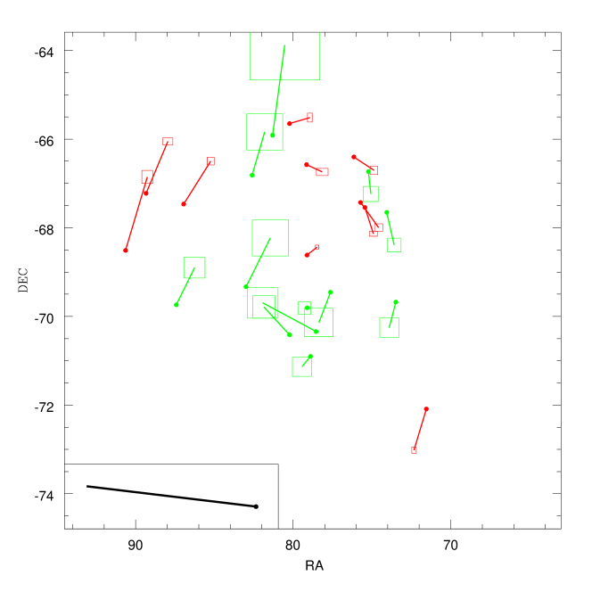
Figure 1.— The spatially variable component ${\vec{\mu}}_{\rm obs,var}$ of the observed LMC PM field. The positions of 22 fields observed with HST are indicated by solid dots. The PM vector shown for each field corresponds to the mean observed absolute PM of the stars in the given field, minus the constant vector ${\vec{\mu}}_{0}$ shown in the inset on the bottom left. The vector ${\vec{\mu}}_{0}$ is our best-fit for the PM of the LMC COM (see Table 1 and Paper I). PMs are depicted by a vector that starts at the field location, with a size that (arbitrarily) indicates the mean predicted motion over the next $7.2\>{\rm Myr}$. Clockwise motion is clearly evident. The uncertainty in each PM vector is illustrated by an open box centered on the end of each PM vector, which depicts the region $\pm\xi\Delta\mu_{W}$ by $\pm\xi\Delta\mu_{N}$. The constant $\xi=1.36$ was chosen such that the box contains $68.3$% of the two-dimensional Gaussian probability distribution. High-accuracy fields (with long time baselines, three epochs of data, and small error boxes) are shown in red, while low-accuracy fields (with short time baselines, two epochs of data, and larger error boxes) are shown in green. The figure shows an (RA,DEC) representation of the sky, with the horizontal and vertical extent representing an equal number of degrees on the sky. The figure is centered on the PM dynamical center $(\alpha_{0},\delta_{0})$ of the LMC, as derived in the present paper (see Table 1).

2.2. Velocity Field Model

To interpret the LMC PM observations one needs a model for the PM vector ${\vec{\mu}}=(\mu_{W},\mu_{N})$ as a function of position on the sky. The PM model can be expressed as a function of equatorial coordinates, ${\vec{\mu}}_{\rm mod}(\alpha,\delta)$, or as a function of polar coordinates, ${\vec{\mu}}_{\rm mod}(\rho,\Phi)$, where $\rho$ is the angular distance from the LMC COM and $\Phi$ is the corresponding position angle measured from North over East. Generally speaking, the model can be written as a sum of two vectors, ${\vec{\mu}}_{\rm mod}={\vec{\mu}}_{\rm sys}+{\vec{\mu}}_{\rm rot}$, representing the contributions from the systemic motion of the LMC COM and from the internal rotation of the LMC, respectively.

Consider first the contribution from the systemic motion. The three-dimensional velocity that determines how the LMC COM moves through space is a fixed vector. However, the projection of this vector onto the West and North directions depends on where one looks in the LMC. This introduces an important spatial variation in the PM field, due to several different effects, including: (i) only a fraction $\cos(\rho)$ of the LMC transverse velocity is seen in the PM direction; (ii) a fraction $\sin(\rho)$ of the LMC LOS velocity is also seen in the PM direction; and (iii) the directions of West and North are not fixed in a zenithal projection centered on the LMC, due to the deviation of $(\alpha,\delta)$ contours from an orthogonal grid near the South Galactic pole (see figure 4 of van der Marel & Cioni 2001, hereafter vdMC01). As a result, one can write ${\vec{\mu}}_{\rm sys}(\alpha,\delta)={\vec{\mu}}_{0}+{\vec{\mu}}_{\rm per}(\alpha,\delta)$. The first term is the constant PM of the LMC COM, measured at the position of the COM. The second term is the spatially varying component of the systemic contribution, which can be referred to as the “viewing perspective” component.

To describe the component of internal rotation, we assume that the LMC is a flat disk with circular streamlines. This is the same approach that has been used successfully to model LOS velocities in the LMC (e.g., vdM02; O11). However, it should be kept in mind that this model is only approximately correct. The LMC is not circular in its disk plane (vdM01), so the streamlines are not expected to be exactly circular. Fortunately, the gravitational potential is always rounder than the density distribution, so circular streamlines should give a reasonable low-order approximation. Also, the modest $V/\sigma$ of the LMC indicates that its disk is not particularly thin (vdM02). So the flat-disk model should be viewed as an approximation to the actual (three-dimensional) velocity field as projected onto the disk plane.

At any point in the disk, the relation between the transverse velocity $v_{t}$ in km/s and the PM $\mu$ in mas/yr is given by $\mu=v_{t}/(4.7403885D)$, where $D$ is the distance in kpc. The distance $D$ is not the same for all fields, and is not the same as the distance $D_{0}$ of the LMC COM. The LMC is an inclined disk, so one side of the LMC is closer to use than the other. This has been quantified explicitly by comparing the relative brightness of stars on opposite sides of the LMC (e.g., vdMC01).

The analytical expressions for the PM field thus obtained,

$${\vec{\mu}}_{\rm mod}(\alpha,\delta)={\vec{\mu}}_{\rm 0}+{\vec{\mu}}_{\rm per}(\alpha,\delta)+{\vec{\mu}}_{\rm rot}(\alpha,\delta),$$ (1)

were presented in vdM02. We refer the reader to that paper for the details of the spherical trigonometry and linear algebra involved. The following model parameters uniquely define the model:

• The projected position $(\alpha_{0},\delta_{0})$ of the LMC COM, which is also the dynamical center of the LMC’s rotation.

• The orientation of the LMC disk, as defined by the inclination $i$ (with $0^{\circ}$ defined as face-on) and the position angle $\Theta$ of the line of nodes (the intersection of the disk and sky planes), measured from North over East.

• The PM of the LMC COM, $(\mu_{W0},\mu_{N0})$, expressed in the heliocentric frame (i.e., not corrected for the reflex motion of the Sun).

• The heliocentric LOS velocity of the LMC COM, $v_{\rm LOS,0}/D_{0}$, expressed in angular units (for which we use mas/yr throughout this paper).

• The rotation curve in the disk, $V(R^{\prime})/D_{0}$, expressed in angular units. Here $R$ is the radius in the disk in physical units, and $R^{\prime}\equiv R/D_{0}$. (Along the line of nodes, $R^{\prime}=\tan(\rho)$; in general, the LMC distance must be specified to calculate the radius in the disk is in physical units).

The first two bullets define the geometrical properties of the LMC, and the last three bullets its kinematical properties.

Figures 10a,b of vdM02 illustrate the predicted morphology of the PM fields $\mu_{\rm per}$ and $\mu_{\rm rot}$ for a specific LMC model tailored to fit the LOS velocity field. These two components have comparable amplitudes. The spatially variable component of the observed PM field ${\vec{\mu}}_{\rm obs,var}$ in Figure 1 provides an observational estimate of the sum ${\vec{\mu}}_{\rm per}+{\vec{\mu}}_{\rm rot}$ (compare eq. [1]).

2.3. Information Content of the Proper Motion and Line-of-Sight Velocity Fields

The PM field is defined by the variation of two components of motion over the face of the LMC. By contrast, the LOS velocity field is defined by the variation of only one component of motion. The PM field therefore contains more information, and has more power to discriminate the parameters of the model. As we will show, important constraints can be obtained with only 22 PM measurements, whereas LOS velocity studies require hundreds or thousands of stars.

The following simple arguments show that knowledge of the full PM field in principle allows unique determination of all model parameters, without degeneracy.

• The dynamical center $(\alpha_{0},\delta_{0})$ is the position around which the spatially variable component of the PM field has a well-defined sense of rotation.

• The azimuthal variation of the PM rotation field determines both of the LMC disk orientation angles $(\Theta,i)$. Perpendicular to the line of nodes (i.e., $\Phi=\Theta\pm 90^{\circ}$), all of the rotational velocity $V(R^{\prime})$ in the disk is seen as a PM (and none is seen along the LOS). By contrast, along the line of nodes (i.e., $\Phi=\Theta$ or $\Theta+180^{\circ}$), only approximately $V(R^{\prime})\cos i$ is seen as a PM (and approximately $V(R^{\prime})\sin i$ is seen along the LOS). The near and far side of the disk are distinguished by the fact that velocities on the near side imply larger PMs.

• The PM of the LMC COM, $(\mu_{W0},\mu_{N0})$, is the PM at the dynamical center.

• The systemic LOS velocity $v_{\rm LOS,0}/D_{0}$ in angular units follows from the radially directed component of the PM field. A fraction $\sin(\rho)v_{\rm LOS,0}$ is seen in this direction (appearing as an “inflow” for $v_{\rm LOS,0}>0$ and an “outflow” for $v_{\rm LOS,0}<0$). This component is almost perpendicular to the more tangentially oriented component induced by rotation in the LMC disk, so the two are not degenerate. However, the radially directed component is small near the galaxy center (e.g., $\sin(\rho)\lesssim 0.07$ for $\rho\lesssim 4^{\circ}$), so exquisite PM data would be required to constrain $v_{\rm LOS,0}/D_{0}$ with meaningful accuracy.

• The rotation curve $V(R^{\prime})/D_{0}$ in angular units follows from the PMs along the line-of-nodes position angle $\Theta$.

Table 1LMC Model Parameters: New Fit Results from Three-Dimensional Kinematics

Quantity	Unit	PMs	PMs+Old	PMs+Young
			$v_{\rm LOS}$ sample	$v_{\rm LOS}$ sample
(1)	(2)	(3)	(4)	(5)
$\alpha_{0}$	deg	$78.76\pm 0.52$	$79.88\pm 0.83$	$80.05\pm 0.34$
$\delta_{0}$	deg	$-69.19\pm 0.25$	$-69.59\pm 0.25$	$-69.30\pm 0.12$
$i$	deg	$39.6\pm 4.5$	$34.0\pm 7.0$	$26.2\pm 5.9$
$\Theta$	deg	$147.4\pm 10.0$	$139.1\pm 4.1$	$154.5\pm 2.1$
$\mu_{W0}$	mas/yr	$-1.910\pm 0.020$	$-1.895\pm 0.024$	$-1.891\pm 0.018$
$\mu_{N0}$	mas/yr	$0.229\pm 0.047$	$0.287\pm 0.054$	$0.328\pm 0.025$
$v_{\rm LOS,0}$	km/s	$262.2\pm 3.4$	$261.1\pm 2.2$	$269.6\pm 1.9$
$V_{0,{\rm PM}}/D_{0}$	mas/yr	$0.320\pm 0.029$	$0.353\pm 0.034$	$0.289\pm 0.025$
$V_{0,{\rm PM}}$	km/s	$76.1\pm 7.6$	$83.8\pm 9.0$	$68.8\pm 6.4$
$V_{0,{\rm LOS}}$	km/s	$\ldots$	$55.2\pm 10.3$	$89.3\pm 18.8$
$V_{0,{\rm LOS}}\>\sin i$	km/s	$\ldots$	$30.9\pm 2.6$	$39.4\pm 1.9$
$R_{0}/D_{0}$		$0.024\pm 0.010$	$0.075\pm 0.005$	$0.040\pm 0.003$
$D_{0}$	kpc	$50.1\pm 2.5\>{\rm kpc}$	$50.1\pm 2.5\>{\rm kpc}$	$50.1\pm 2.5\>{\rm kpc}$

Note. — Column (1) lists the model quantity, and column (2) its units. Column (3) lists the values from the model fit to the PM data in Section 2. Columns (4) and (5) list the values from the model fit to the combined PM and LOS velocity data in Section 3, for the old and young $v_{\rm LOS}$ sample, respectively. From top to bottom, the following quantities are listed: Position $(\alpha_{0},\delta_{0})$ of the dynamical center; Orientation angles $(i,\Theta)$ of the disk plane, being the inclination angle and line-of-nodes position angle, respectively; PM $(\mu_{W0},\mu_{N0})$ of the COM; LOS velocity $v_{\rm LOS,0}$ of the COM; Amplitude $V_{0,{\rm PM}}/D_{0}$ or $V_{0,{\rm PM}}$ of the rotation curve in angular units or physical units, respectively, as inferred from the PM data. Amplitude $V_{0,{\rm LOS}}$ of the rotation curve as inferred from the LOS velocity data, and observed component $V_{0,{\rm LOS}}\>\sin i$. Turnover radius $R_{0}/D_{0}$ of the rotation curve, expressed as a fraction of the distance (the rotation curve being parameterized so that it rises linearly to velocity V0 at radius R0, and then stays flat at larger radii); and the distance $D_{0}$.

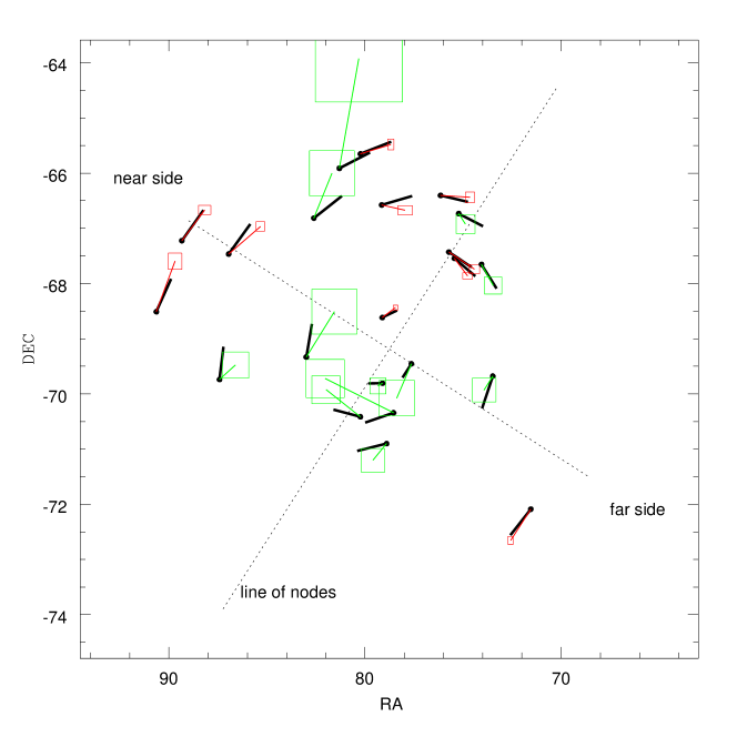
Figure 2.— Data-model comparison for the rotation component ${\vec{\mu}}_{\rm obs,rot}$ of the observed LMC PM field, with similar plotting conventions as in Figure 1. For each field we now show in color the mean observed absolute PM of the stars in the given field, minus the component ${\vec{\mu}}_{\rm sys}={\vec{\mu}}_{0}+{\vec{\mu}}_{\rm per}$ implied by the best-fit model (see Table 1). The latter subtracts the systemic motion of the LMC, and includes not only the PM of the LMC COM (as in Figure 1) but also the spatially-varying viewing perspective component. Solid black vectors show the rotation component ${\vec{\mu}}_{\rm rot}$ of the best-fit model. The observations show clockwise motion, which is reproduced by the model. A dotted line indicates the line of nodes, along position angle $\Theta$. Another dotted line connects the near and the far sides of the LMC disk, along position angles $\Theta-90^{\circ}$ and $\Theta+90^{\circ}$, respectively. Along the near-far direction, PMs are larger by a factor $1/\cos i$ than along the line of nodes. However, distances along the near-far direction are foreshortened by a factor $\cos i$ compared to distances along the line of nodes (as indicated by the length of the dotted lines). The lines intersect at the dynamical center $(\alpha_{0},\delta_{0})$. The geometrical parameters $(\Theta,i,\alpha_{0},\delta_{0})$ are all uniquely defined by the model fit to the data, as is the rotation curve in the disk which is shown in Figure 6.

By contrast, full knowledge of the LOS velocity field does not constrain all the model parameters uniquely. Specifically, there is strong degeneracy between three of the model parameters (see vdM02): the rotation curve $V(R^{\prime})$, the inclination angle $i$ (since the observed LOS velocity component is approximately $V(R^{\prime})\sin i$), and the component $v_{t0c}$ of the transverse COM velocity vector ${\vec{v}}_{t0}$ projected onto the line of nodes (which adds a solid-body component to the observed rotation). So the rotation curve can only be determined from the LOS velocity field if $i$ and $v_{t0c}$ are assumed to be known independently. Typically (e.g., vdM02; O11), $i$ has been estimated from geometric methods (e.g., vdMC01) and $v_{t0c}$ from proper motion studies (e.g., K06). It should be noted that the transverse COM velocity component $v_{t0s}$ in the direction perpendicular to the line of nodes is determined uniquely by the LOS velocity field, as is the position angle $\Theta$ of the line of nodes itself. And of course, the systemic LOS velocity $v_{\rm LOS,0}$ is determined much more accurately by the LOS velocity field than by the PM field.

An important difference between the two observationally accessible fields is that the PM field constrains velocities in angular units (mas/yr), whereas the LOS velocity field constrains the same velocities in physical units (km/s). Hence, comparison of the results for e.g. $V(R^{\prime})$ or $v_{t0s}$ from the two fields constrains the LMC distance $D_{0}$. This is discussed further in Section 4.6.

2.4. Fitting Methodology

In our earlier analysis of K06, we treated $(\mu_{W0},\mu_{N0})$ as the only free parameters to be determined from the PM data. All other quantities were kept fixed to estimates previously obtained either by vdM02 from a study of the LMC LOS velocity field, by vdMC01 from a study of the LMC orientation angles, or by Freedman et al. (2001) from a study of the LMC distance. P08 took the same approach, but as discussed in Section 1, they did treat the rotation curve $V(R^{\prime})$ as a free function to be determined from the data. Keeping model parameters fixed a priori is reasonable when only limited data is available. However, this does have several undesirable consequences. First, it does not use the full information content of the PM data, which actually constrains the parameters independently. Second, it opens the possibility that parameters are used that are not actually consistent with the PM data. And third, it leads to underestimates of the errorbars on the LMC COM PM $(\mu_{W0},\mu_{N0})$, since the uncertainties in the geometry and rotation of the LMC are not propagated into the answers (as discussed in Paper I).

The three-epoch PM data presented in Paper I have much improved quality over the two-epoch measurements presented by K06a and P08, as evident from Figure 1. We therefore now treat all of the key parameters that determine the geometry and kinematics of the LMC as free parameters to be determined from the data. There are $M=22$ LMC fields, and hence $N_{\rm data}=2M=44$ observed quantities (there are two PM coordinates per field). By comparison, the model is defined by the 7 parameters $(\alpha_{0},\delta_{0},\mu_{W0},\mu_{N0},v_{\rm LOS,0}/D_{0},i,\Theta)$ and the one-dimensional function $V(R^{\prime})/D_{0}$. The rotation curves of galaxies follow well-defined patterns, and are therefore easily parameterized with a small number of parameters. We use a very simple form with two parameters

$$V(R^{\prime})/D_{0}=(V_{0}/D_{0})\>\min[R^{\prime}/(R_{0}/D_{0}),\>1)]$$ (2)

(similar to P08 and O11). This corresponds to a rotation curve that rises linearly to velocity $V_{0}$ at radius $R_{0}$, and stays flat beyond that. The quantity $V_{0}/D_{0}$ is the rotation amplitude expressed in angular units. Later in Section 4.5 we also present unparameterized estimates of the rotation curve $V(R^{\prime})$. Sticking with the parameterized form for now, we have an overdetermined problem with more data points ($N_{\rm data}=44$) than model parameters ($N_{\rm param}=9$), so this is a well-posed mathematical problem. We also know from the discussion in Section 2.3 that the model parameters should be uniquely defined by the data without degeneracy. So we proceed by numerical fitting of the model to the data.

To fit the model we define a $\chi^{2}$ quantity

$$\chi^{2}_{\rm PM}\equiv\sum_{i=1}^{M} \left[(\mu_{W,{\rm obs},i}-\mu_{W,{\rm mod},i})/\Delta\mu_{W,{\rm obs},i}\right]^{2}+$$ (3)

$$\left[(\mu_{N,{\rm obs},i}-\mu_{N,{\rm mod},i})/\Delta\mu_{N,{\rm obs},i}\right]^{2}$$

that sums the squared residuals over all $M$ fields. We minimize $\chi^{2}_{\rm PM}$ as function of the model parameters using a down-hill simplex routine (Press et al. 1992). Multiple iterations and checks were built in to ensure that a global minimum was found in the multi-dimensional parameter space, instead of a local minimum.

Table 2LMC Model Parameters: Literature Results from Line-of-Sight Velocity Analyses

Quantity	Unit	vdM02	O11
		(carbon stars)	(RSGs)
e(1)	(2)	(3)	(4)
$\alpha_{0}$	deg	$81.91\pm 0.98$	$81.91\pm 0.98$
$\delta_{0}$	deg	$-69.87\pm 0.41$	$-69.87\pm 0.41$
$i$	deg	$34.7\pm 6.2$	$34.7\pm 6.2$
$\Theta$	deg	$129.9\pm 6.0$	$142\pm 5$
$\mu_{W0}$	mas/yr	$-1.68\pm 0.16$	$-1.956\pm 0.036$
$\mu_{N0}$	mas/yr	$0.34\pm 0.16$	$0.435\pm 0.036$
$v_{\rm LOS,0}$	km/s	$262.2\pm 3.4$	$263\pm 2$
$V_{0,{\rm LOS}}$	km/s	$49.8\pm 15.9$	$87\pm 5$
$V_{0,{\rm LOS}}\>\sin i$	km/s	$28.4\pm 7.9$	$50\pm 3$
$R_{0}/D_{0}$		$0.080\pm 0.004$	$0.048\pm 0.002$
$D_{0}$	kpc	$50.1\pm 2.5\>{\rm kpc}$	$50.1\pm 2.5\>{\rm kpc}$

Note. — Parameters from model fits to LMC LOS velocity data, as obtained by vdM02 and O11; listed in columns (3) and (4), respectively. The table layout and the quantities in column (1) are as in Table 1. Parameter uncertainties are from the listed papers. Many of these are underestimates, for the reasons stated in the footnotes.

Once the best-fitting model parameters are identified, we calculate error bars on the model parameters using Monte Carlo simulations. Many different pseudo–data sets are created that are analyzed similarly to the real data set. The dispersions in the inferred model parameters are a measure of the $1\sigma$ random errors on the model parameters. Each pseudo–data set is created by calculating for each observed field the best-fit model PM prediction, and by adding to this random Gaussian deviates. The deviates are drawn from the known observational error bars, multiplied by a factor $(\chi^{2}_{\rm min}/N_{DF})^{1/2}$. Here $\chi^{2}_{\rm min}$ is the $\chi^{2}_{\rm PM}$ value of the best-fit model, and $N_{\rm DF}=N_{\rm data}-N_{\rm param}+N_{\rm fixed}$ is the number of degrees of freedom, with $N_{\rm fixed}$ the number of parameters (if any) that are not optimized in the fit. In practice we find that $\chi^{2}_{\rm min}$ is somewhat larger than $N_{DF}$, indicating that the actual scatter in the data is slightly larger than what is accounted for by random errors. This is not surprising, given the complexity of the astrometric data analysis and the relative simplicity of the model. The approach used to create the pseudo-data ensures that the actual scatter is propagated into the final uncertainties on the model parameters.

It is known from LOS velocity studies that $v_{\rm LOS,0}=262.2\pm 3.4\ {\rm{km\ s^{-1}}}\>$ (vdM02), and from stellar population studies that $D_{0}=50.1\pm 2.5$ kpc ($m-M=18.50\pm 0.10$; Freedman et al. 2001). So $v_{\rm LOS,0}$ is known to $\sim 1\%$ accuracy and $D$ to $\sim 5\%$ accuracy. Not surprisingly, we have found that the PM data cannot constrain the model parameter $v_{\rm LOS,0}/D_{0}$ with similar accuracy. Therefore, we have kept $v_{\rm LOS,0}/D_{0}$ fixed in our analysis to the value implied by existing knowledge. At $m-M=18.50$, 1 mas/yr corresponds to $237.58\ {\rm{km\ s^{-1}}}\>$. Hence, $v_{\rm LOS,0}/D_{0}=1.104\pm 0.053$ mas/yr. The uncertainty in this value was propagated into the analysis by using randomly drawn $v_{\rm LOS,0}/D_{0}$ values in the fitting of the different Monte-Carlo generated pseudo-data sets.

2.5. Data-Model Comparison

Table 1 lists the parameters of the best-fit model and their uncertainties. These parameters are discussed in detail in Section 4. Figure 2 shows the data-model comparison for the best fit. For this figure, we subtracted the systemic velocity contribution ${\vec{\mu}}_{\rm sys}={\vec{\mu}}_{0}+{\vec{\mu}}_{\rm per}$ implied by the best-fit model, from both the observations and the model. By contrast to Figure 1, this now also subtracts the spatially-varying viewing perspective. So the observed rotation component ${\vec{\mu}}_{\rm obs,rot}\equiv{\vec{\mu}}_{\rm obs}-{\vec{\mu}}_{0}-{\vec{\mu}}_{\rm per}$ is compared to the model component ${\vec{\mu}}_{\rm rot}$. Clockwise motion is clearly evident in the observations, and this is reproduced by the model.

The best-fit model has $\chi^{2}_{\rm min}=116.0$ for $N_{DF}=36$. Hence, $(\chi^{2}_{\rm min}/N_{DF})^{1/2}=1.80$. So even though the model captures the essence of the observations, it is not formally statistically consistent with it. There are three possible explanations for this. First, the observations could be affected by unidentified low-level systematics in the data analysis, in addition to the well-quantified random uncertainties. Second, shot noise from the finite number of stars may be important for some fields with low $N$, causing the mean PM of the observed stars to deviate from the true mean motion in the LMC disk. And third, the model may be too over-simplified (e.g., if there are warps in the disk, or if the streamlines in the LMC disk deviate from circles at a level comparable to our measurement uncertainties). It is difficult to establish which explanation may be correct, and the explanation may be different for different fields.

Two of our HST fields are close to each other at a separation of only $0.16^{\circ}$, and this provides some additional insight into potential sources of error. The fields, labeled L12 and L14 in table 1 of Paper I, are located at $\alpha\approx 75.6^{\circ}$ and $\delta\approx-67.5^{\circ}$ (see Figure 1). Since the fields are so close to each other, the best-fit model predicts that the PMs should be similar, ${\vec{\mu}}_{\rm mod,L12}-{\vec{\mu}}_{\rm mod,L14}=(-0.015,-0.031)$ mas/yr. However, the observations differ by ${\vec{\mu}}_{L12}-{\vec{\mu}}_{L14}=(-0.110\pm 0.047,-0.001\pm 0.037)$ mas/yr. This level of disagreement can in principle happen by chance (9% probability), but maybe a possible additional source of error is to blame. The disagreement in this case cannot arise because the model is too oversimplified, since almost any model would predict that closely-separated fields in the disk have similar PMs. Also, shot noise is too small to explain the difference. These fields had $N=16$–18 stars measured, and a typical velocity dispersion in the disk is $\sigma\approx 20\ {\rm{km\ s^{-1}}}\>$ (vdM02). This implies a shot noise error (per coordinate, per field) of only $\sim 0.02$ mas/yr, which is below the random errors for these fields. These fields have lower $N$ and smaller random errors than most other fields, so this means that shot noise in general plays at most a small role. So in the case of these fields, and maybe for the sample as a whole, it is likely that we are dealing with unidentified low-level systematics in the data analysis.

Either way, the exact cause why $\chi^{2}_{\rm min}>N_{DF}$ does not matter much, since in the Monte-Carlo analysis of pseudo-data we multiply all observational errors by $(\chi^{2}_{\rm min}/N_{DF})^{1/2}$. So the actual residuals in the data-model comparison are accounted for when calculating the uncertainties in the model parameters. Moreover, the astrometric observations presented in Paper I are extremely challenging. So the level of agreement in the data-model comparison of Figure 2 is actually extremely encouraging.

3. Line-of-Sight Rotation Field

Many studies exist of the LOS velocity field of tracers in the LMC, as discussed in Section 1. Two of the most sophisticated studies are those of vdM02 and O11. The vdM02 study modeled the LOS velocities of $\sim 1000$ carbon stars, and its results formed the basis of the rotation model used in K06. The more recent O11 study obtained a rotation fit to the LOS velocities of $\sim 700$ red supergiants (RSGs), and also presented $\sim 4000$ new LOS velocities for other giant and AGB stars. The parameters of the vdM02 and O11 rotation models are presented in Table 2.

Comparison of the vdM02 and O11 parameters to those obtained from our PM field fit in Table 1 shows a few important differences. The COM PM values used by both vdM02 and O11 are inconsistent with our most recent estimate from Paper I. This is important, because the transverse motion of the LMC introduces a solid body rotation component into the LMC LOS velocity field, which must be corrected to model the internal LMC rotation. Also, the dynamical centers either inferred (vdM02) or used (O11) by the past LOS velocity studies are in conflict with the dynamical center implied by the new PM analysis. These differences are discussed in detail in Section 4. Motivated by these differences, we decided to perform a new analysis of the available LOS velocity data from the literature, taking into account the new PM results. This yields a full three-dimensional view of the rotation of the LMC disk.

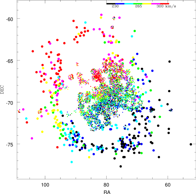
Figure 3.— LMC LOS velocity field defined by 6790 observed stellar velocities available from the literature. All stars in the combined young and old samples discussed in the text are shown. Each star is color-coded by its velocity according to the legend at the top. Most of the stars at large radii are carbon stars from the study of Kunkel et al. (1997); these stars are shown with larger symbols. A velocity gradient is visible by eye, and this is modeled in Section 3 to constrain rotation models for the LMC. The area shown in this figure is larger than that in Figures 1, 2, and 5.

3.1. Data

It is well-known that the kinematics of stars in the LMC depends on the age of the population, as it does in the Milky Way. Young populations have small velocity dispersions, and high rotation velocities. By contrast, old populations have higher velocity dispersions (e.g., van der Marel et al. 2009), and lower rotation velocities (see Table 4) due to asymmetric drift. For this reason, we compiled two separate samples from the literature for the present analysis: a “young” sample and an “old” sample. The young sample is composed of RSGs, which is the youngest stellar population for which detailed accurate kinematical data exist. The old sample is composed of a mix of carbon stars, AGB stars, and RGB stars.

For our young sample, we combined the RSG velocities of Prevot et al. (1985), Massey & Olsen (2003), and O11 (adopting the classification from their figure 1). For the old sample, we combined the carbon star velocities of Kunkel et al. (1997), Hardy et al. (2001; as used also by vdM02), and O11; the oxygen-rich and extreme AGB star velocities of O11; and the RGB star velocities of Zhao et al. (2003; selected from their figure 1 using the color criterion $B-R>0.4$), Cole et al. (2005), and Carrera et al. (2011).

When a star is found in more than one dataset, we retained only one of the multiple velocity measurements. If a measurement existed from O11, we retained that, because the O11 data set is the largest and most homogeneous dataset available. Otherwise we retained the measurement from the data set with the smallest random errors.

Stars with non-conforming velocities were rejected iteratively using outlier rejection. For the young and old samples we rejected stars with velocities that differ by more than $45\ {\rm{km\ s^{-1}}}\>$ and $90\ {\rm{km\ s^{-1}}}\>$ from the best-fit rotation models, respectively. In each case this corresponds to residuals $\gtrsim 4\sigma$, where $\sigma$ is the LOS velocity dispersion of the sample. The outlier rejection removes both foreground Milky Way stars, as well as stripped SMC stars that are seen in the direction of the LMC (estimated by O11 as $\sim 6$% of their sample).

All samples were brought to a common velocity scale by applying additive velocity corrections to the data for each sample. These were generally small, except for the Zhao et al. (2003) sample. We adopted the absolute velocity scale of O11 as the reference. Since they observed both young and old stars in the same fields with the same setup, this ties together the velocity scales of the young and old samples. To bring other samples to the O11 scale we used stars in common between the samples, and we also compared the residuals relative to a common velocity field fit.

Our final samples contain LOS velocities for 723 young stars and 6067 old stars in the LMC. Figure 3 shows a visual representation of the discrete velocity field defined by the stars in the combined sample. The coverage of the LMC is patchy and incomplete, as defined by the observational setups used by the various studies. The young star sample is confined almost entirely to distances $\lesssim 4$ degrees from the LMC center. This is where the old star sample has most of its measurements as well. However, a sparse sampling of old star velocities does continue all the way out to $\sim 14$ degrees from the LMC center. A velocity gradient is easily visible in the figure by eye. What is observed is the sum of the internal rotation of the LMC and an apparent solid-body rotation component due to the LMC’s transverse motion (vdM02). The latter component contributes more as one moves further from the LMC center, which causes an apparent twisting of the velocity field with radius.

3.2. Fitting Methodology

To interpret the LOS velocity data we use the same rotation field model for a circular disk as in Section 2.2. The model is defined by the 7 parameters $(\alpha_{0},\delta_{0},D_{0}\mu_{W0},D_{0}\mu_{N0},v_{\rm LOS,0},i,\Theta)$ and the one-dimensional function $V(R^{\prime})$, which we parameterize with the two parameters $V_{0}$ and $R_{0}$ as in equation (2). Note that the LOS velocity field depends on the physical velocities $v_{W0}\equiv D_{0}\mu_{W0}$, $v_{N0}\equiv D_{0}\mu_{N0}$, $v_{\rm LOS,0}$, and $V(R^{\prime})$, unlike the PM field, which depends on the angular velocities $\mu_{W0}$, $\mu_{N0}$, $v_{\rm LOS,0}/D_{0}$, and $V(R^{\prime})/D_{0}$. As before, the model can be written as a sum of two terms, $v_{\rm LOS,mod}=v_{\rm LOS,sys}+v_{\rm LOS,rot}$, representing the contributions from the systemic motion of the LMC COM and from the internal rotation of the LMC, respectively. The analytical expressions for the LOS velocity field $v_{\rm LOS,mod}(\alpha,\delta)$ thus obtained were presented in vdM02. As before, we refer the reader to that paper for the details of the spherical trigonometry and linear algebra involved.

In Section 2 we have fit the PM data by themselves, and in other studies such as vdM02 and O11, the LOS data have been fit by themselves. These approaches require that some systemic velocity components ($v_{\rm LOS,0}$ for the PM field analysis, and $(\mu_{W0},\mu_{N0})$ for the LOS velocity field analysis) must be fixed a priori to literature values. But clearly, the best way to use the full information content of the data is to fit the PM and LOS data simultaneously. This is therefore the approach we take here.

To fit the combined data, we define a $\chi^{2}$ quantity

$$\chi^{2}\equiv\chi^{2}_{\rm PM}+\chi^{2}_{\rm LOS}.$$ (4)

The quantity $\chi^{2}_{\rm PM}$ is as defined in equation (3). The observational PM errors are adjusted as in Section 2.5 so that the best fit to the PM data by themselves yields $\chi^{2}_{\rm PM}=N_{\rm DF}$. Similarly, we define

$$\chi^{2}_{\rm LOS}\equiv\sum_{i=1}^{N}\left[(v_{{\rm LOS,obs},i}-v_{{\rm LOS,mod},i})/\sigma_{\rm LOS,obs}\right]^{2},$$ (5)

which sums the squared residuals over all $N$ LOS velocities. Here $\sigma_{\rm LOS,obs}$ is a measure of the observed LOS velocity dispersion of the sample, which we assume to be a constant for each LOS velocity sample. We set $\sigma_{\rm LOS,obs}$ to be the RMS scatter around the best-fit model that is obtained when the LOS data are fit by themselves (this yields $\chi^{2}_{\rm LOS}=N$, analogous to the case for $\chi^{2}_{\rm PM}$).

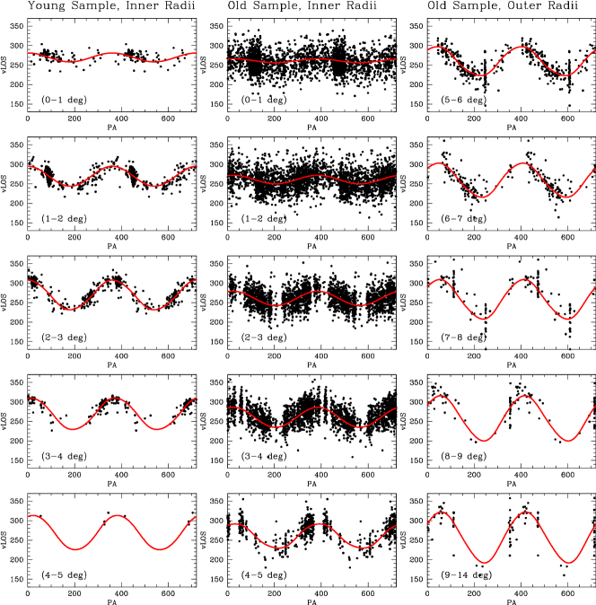
Figure 4.— Data-model comparison for LOS velocities available from the literature. Each panel shows the heliocentric velocity of observed stars as function of the position angle $\Phi$ on the sky. The displayed range of the angle $\Phi$ is $0^{\circ}$–$720^{\circ}$, so each star is plotted twice. The left column is for the young star sample described in the text; the middle and right columns are for the old star sample. Each panel corresponds to a different range of angular distances $\rho$ from the LMC center, as indicated. The curves show the predictions of the best-fit models (calculated at the center of the radial range for the given panel), that also fit the new PM data.

This approach yields that $\sigma_{\rm LOS,obs}=11.6\ {\rm{km\ s^{-1}}}\>$ for the young sample, and $\sigma_{\rm LOS,obs}=22.8\ {\rm{km\ s^{-1}}}\>$ for the old sample. This confirms, as expected, that the older stars have a larger velocity dispersion. These results are broadly consistent with previous work (e.g., vdM02; Olsen & Massey 2007). Note that $\sigma_{\rm LOS,obs}$ represents a quadrature sum of the intrinsic velocity dispersion $\sigma_{\rm LOS}$ of the stars and the typical observational measurement error $\Delta v_{\rm LOS}$. For all the data used here, $\Delta v_{\rm LOS}\ll\sigma_{\rm LOS}$, so it is justified to not include the individual measurement errors $\Delta v_{{\rm LOS},i}$ explicitly in the definition of $\chi^{2}_{\rm LOS}$.

As before, we minimize $\chi^{2}$ as function of the model parameters using a down-hill simplex routine (Press et al. 1992), with multiple iterations and checks built in to ensure that a global minimum is found. We calculate error bars on the best-fit model parameters using Monte Carlo simulations. The pseudo PM data for this are generated as in Section 2.4. The pseudo LOS velocity data are obtained by drawing new velocities for the observed stars. For this we use the predictions of the best-fit model, to which we add random Gaussian deviates that have the same scatter around the fit as the observed velocities.

In minimizing $\chi^{2}$, we treat all model parameters as free parameters that are used to optimize the fit. However, we keep the distance fixed at $m-M=18.50$ (Freedman et al. 2001). The uncertainty $\Delta(m-M)=0.1$ is accounted for by including it in the Monte-Carlo simulations that determine the uncertainties on the best-fit parameters. As discussed later in Section 4.6, the combination of PM and LOS data does constrain the distance independently. However, this does not (yet) yield higher accuracy than conventional methods.

The stars for which we have measured PMs form essentially a magnitude limited sample, composed of a mix of young and old stars. This mix is expected to have a different rotation velocity than a sample composed entirely of young or old stars. For this reason, we allow the rotation amplitude $V_{0,{\rm PM}}$ in the PM field model to be different from the rotation amplitude $V_{0,{\rm LOS}}$ in the velocity field model. Both amplitudes are varied independently to determine the best-fit model. However, we do require the scale length $R_{0}$ of the rotation curve and also the parameters that determine the orientation and dynamical center of the disk to be the same for the PM and LOS models.

With this methodology, we do two separate fits. The first fit is to the combination of the PM data and the young LOS velocity sample, and the second fit is to the combination of the PM data and the old LOS velocity sample. This has the advantage (compared to a single fit to all the data, with only a different rotation amplitude for each sample) of providing two distinct answers. Comparison of the results then provides insight into both the systematic accuracy of the methodology, and potential differences in geometrical or kinematical properties between different stellar populations.

3.3. Data-Model Comparison

Table 1 lists the parameters of the best-fit model and their uncertainties. The quality of the model fits to the PM data is similar to what was shown already in Figure 2 for fits that did not include any LOS velocity constraints. A data-model comparison for the fits to the LOS velocity data is shown in Figure 4. The fits are adequate. It is clear that the young stars rotate more rapidly than the old stars, and have a smaller LOS velocity dispersion. The continued increase in the observed rotation amplitude with radius is due to the solid-body rotation component in the observed velocity field that is induced by the transverse motion of the LMC.

The parameters for the best fit models to the combined PM and LOS velocity samples can be compared to the results obtained when only the PMs are fit (Table 1), or the results that have been obtained in the literature when only the LOS velocities were fit (Table 2). This shows good agreement for some quantities, and interesting differences for others. We proceed in Section 4 by discussing the results and their comparisons in detail, and what they tell us about the LMC.

4. LMC Geometry, Kinematics, and Structure

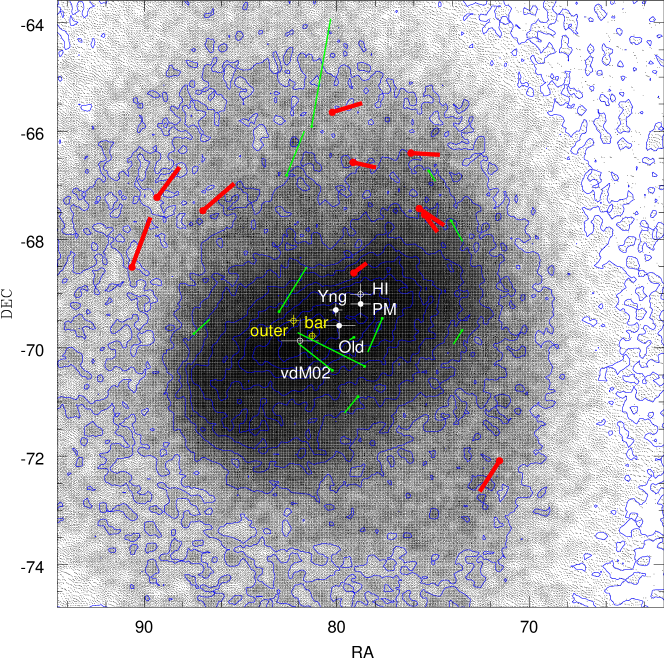
Figure 5.— Determinations of dynamical and photometric centers of the LMC, overplotted on a grey-scale image with overlaid contours (blue) of the number density distribution of old stars in the LMC (extracted from the 2MASS survey; vdM01). Each center is discussed in the text, and is indicated as a circle with error bars. Solid circles are from the present paper (Table 1), while open circles are from the literature. White circles are dynamical centers, while yellow circles are photometric centers. Labels are as follows. PM: stellar dynamical center inferred from the model fit to the new PM data; Old/Yng: stellar dynamical center inferred from the model fit to the combined sample of new PM data and old/young star LOS velocities; vdM02: stellar dynamical center previously inferred from the LOS velocity field of carbon stars; HI: gas dynamical center of the cold HI disk (Luks & Rohlfs 1992; Kim et al. 1998); bar: densest point in the bar (de Vaucouleurs & Freeman 1972; vdM01); outer: center of the outer isoplets, corrected for viewing perspective (vdM01). The rotation component ${\vec{\mu}}_{\rm obs,rot}$ of the observed LMC PM field is overplotted with similar conventions as in Figure 2. The three-epoch data (red) have significantly smaller uncertainties than the two-epoch data (green), but the actual uncertainties are shown only in Figure 2.

4.1. Dynamical Center

The LMC is morphologically peculiar in its central regions, with a pronounced asymmetric bar. Moreover, the light in optical images is dominated by the patchy distribution of young stars and dust extinction. As a result, the LMC has become known as a prototype of “irregular” galaxies (e.g., de Vaucouleurs & Freeman 1972). However, the old stars that dominate the mass of the LMC show a much more regular large-scale morphology. This is illustrated in Figure 5, which shows the number density distribution of red giant and AGB stars extracted from the 2MASS survey (vdM01). Despite this large-scale regularity, there does not appear to be a single well-defined center. It has long been known that different methods and tracers yield centers that are not mutually consistent, as indicated in the figure.

The densest point in the LMC bar is located asymmetrically within the bar, on the South-East side at $(\alpha_{\rm bar},\delta_{\rm bar})=(81.28^{\circ}\pm 0.24^{\circ},-69.78^{\circ}\pm 0.08^{\circ})$ (vdM01; de Vaucouleurs & Freeman 1972). The center of the outer isoplets in Figure 5, corrected for the effect of viewing perspective, is at $(\alpha_{\rm outer},\delta_{\rm outer})=(82.25^{\circ}\pm 0.31^{\circ},-69.50^{\circ}\pm 0.11^{\circ})$ (vdM01). This is on the same side of the bar, but is offset by $0.44^{\circ}\pm 0.14^{\circ}$. By contrast, the dynamical center of the rotating HI disk of the LMC is on the opposite side of the bar, at $(\alpha_{\rm HI},\delta_{\rm HI})=(78.77^{\circ}\pm 0.54^{\circ},-69.01^{\circ}\pm 0.19^{\circ})$ (Kim et al. 1998; Luks & Rohlfs 1992). This is $1.18^{\circ}\pm 0.21^{\circ}$, i.e., more than 1 kpc, away from the densest point in the bar ($1\>{\rm kpc}=1.143^{\circ}$ at $D_{0}=50.1\>{\rm kpc}$).

These offsets do not pose much of a conundrum. Numerical simulations have established that an asymmetric density distribution and offset bar in the LMC can be plausibly induced by tidal interactions with the SMC (e.g., Bekki et al. 2009; Besla et al. 2012). What has been more puzzling is the position of the stellar dynamical center at $(\alpha_{\rm LOS},\delta_{\rm LOS})=(81.91^{\circ}\pm 0.98^{\circ},-69.87^{\circ}\pm 0.41^{\circ})$, as determined by vdM02 from the LOS velocity field of carbon stars. Olsen & Massey (2007) independently fit the same data, and obtained a position (and other velocity field fit parameters) consistent with the vdM02 value. The vdM02 stellar dynamical center was adopted by subsequent studies of LOS velocities (e.g., O11) and PMs (K06, P08), without independently fitting it. This position is consistent with the densest point of the bar and with the center of the outer isophotes. But it is $1.41^{\circ}\pm 0.43^{\circ}$ away from the HI dynamical center. vdM02 argued that this may be due to the fact that HI in the LMC is quite disturbed, and may be subject to non-equilibrium gas-dynamical forces. However, more recent numerical simulations in which the morphology of the LMC is highly disturbed due to interactions with the SMC have shown that the dynamical centers of the gas and stars often stay closely aligned (Besla et al. 2012).

The best-fit stellar dynamical center from our model fit to the PM field is at $(\alpha_{0},\delta_{0})=(78.76^{\circ}\pm 0.52^{\circ},-69.19^{\circ}\pm 0.25^{\circ})$. This agrees with the HI dynamical center (see Figure 5). But it differs from the stellar dynamical center inferred by vdM02 by $1.31^{\circ}\pm 0.44^{\circ}$, which is inconsistent at the 99% confidence level. This is surprising, because the PM field and LOS velocity field are simply different projections of the three-dimensional velocity field of the stellar population. So one would expect the inferred dynamical centers to be the same.

When we fit the PM data and LOS velocities simultaneously (Section 3), we find centers that are somewhat intermediate between between the PM-only dynamical center, and the vdM02 dynamical center (see Figure 5). This is a natural outcome, as these model fits try to compromise between datasets that apparently prefer different centers. The old star sample that we use here is some six times larger than the sample used by vdM02, and yields a center that is consistent with the young star sample used here. Hence, the fact that LOS velocities prefer a stellar dynamical center more towards the South-East of the bar is a generic result, and does not appear to be due to some peculiarity with the carbon star sample used by vdM02. However, the dynamical centers that we infer from the combined PM and LOS samples are much closer to the HI dynamical center than the vdM02 dynamical center. Specifically, the offsets from the HI center are $0.70^{\circ}\pm 0.33^{\circ}$ for the old $v_{\rm LOS}$ sample and $0.54^{\circ}\pm 0.22^{\circ}$ for the young $v_{\rm LOS}$ sample. Such offsets occur by chance only 9% and 6% of the time, respectively. Hence, they most likely signify a systematic effect and not just a chance occurrence.

In reality, it is likely that the HI and stellar dynamical centers are coincident, since both the stars and the gas orbit in the same gravitational potential. Some unknown systematic effect may therefore be affecting the LOS velocity analyses. For example, there is good reason to believe that the true dynamical structure of the LMC is more complicated than the circular orbits in a thin plane used by our models (e.g., warps and twists of the disk plane have been suggested by vdMC01, Olsen & Salyk 2002, and Nikolaev et al. 2004). The uncertainties thus introduced may well affect different tracers differently, leading to systematic offsets such as those reported here. Visual inspection of the PM vector field in Figure 2 strongly supports that the center of rotation must be close to the position identified by the PM-only model fit. For example, the PM vectors in the central region do not have a definite sense of rotation around the position identified by vdM02. Visual inspection of the LOS velocity field in Figure 4 shows the difficulty of determining an accurate center from such data. Either way, the results in Table 1 and Figure 5 definitely indicate the LMC stellar dynamical center is much closer to the HI dynamical center than was previously believed.

4.2. Disk Orientation

Existing constraints on the orientation of the LMC disk come from two techniques. The first technique is a geometric one, based on variations in relative distance to tracers in different parts of the LMC disk (vdMC01). The second is a kinematic method, based on fitting circular orbit models to the velocity field of tracers, as we have done here. The geometric technique yields both the inclination and line-of-nodes position angle. When applied to LOS velocities, the kinematic technique yields only the line-of-nodes position angle, since the inclination is degenerate with the amplitude of the rotation curve. But when applied to PMs, the kinematic technique yields both viewing angles (see Section 2.3).

Existing constraints on the disk orientation obtained with these techniques were reviewed in, e.g., van der Marel (2006) and van der Marel et al. (2009). Some more recent results have appeared in e.g. Koerwer (2009), O11, Haschke et al. (2012), Rubele et al. (2012), and Subramanian & Subramaniam (2013). All studies in the past decade or so agree that the inclination is in the range $i\approx 25^{\circ}$–$40^{\circ}$, and that the line-of-nodes position angle is in the range $\Theta\approx 120^{\circ}$–$155^{\circ}$. However, the variations between the results from different studies are large, and often exceed significantly the random errors in the best-fit parameters. Some of this variation may be real, and due to spatial variations in the viewing angles due to warps and twists of the disk plane, combined with differences in spatial sampling between studies, differences between different tracer populations, and contamination by possible out of plane structures (e.g., O11).

Our best-fit model to the PM velocity field has $i=39.6^{\circ}\pm 4.5^{\circ}$ and $\Theta=147.4^{\circ}\pm 10.0^{\circ}$. The implied viewing geometry of the disk is illustrated in Figure 2. The inferred orientation angles are within the range of expectation based on previous work, although they are at the high end. However, they are perfectly plausible given what is known about the LMC. This is an important validation of the accuracy of the PM data and of our modeling techniques. It is the first time that PMs have been used to derive the viewing geometry of any galaxy. However, the random errors in our estimates are not sufficiently small to resolve the questions left open by past work (apart from the fact that variations in previously reported values appear to be dominated by systematic variations, and not random errors).

When we fit not only the PM data, but also LOS velocities, the best-fit viewing angles change (Table 1), in some cases by more than the random errors. However, all inferred values continue to be within the range of what has been reported in the literature. The best-fit inclination with PM data and the old star $v_{\rm LOS}$ sample is $i=34.0^{\circ}\pm 7.0^{\circ}$, consistent e.g. with the value $i=34.7^{\circ}\pm 6.2^{\circ}$ inferred geometrically by vdMC01 (and used subsequently in the kinematical studies of vdM02 and O11). The best-fit line-of-nodes position angle with the PM data and the old star $v_{\rm LOS}$ sample is $\Theta=139.1^{\circ}\pm 4.1^{\circ}$. This is somewhat larger than the carbon star result $\Theta=129.9^{\circ}\pm 6.0^{\circ}$ obtained by vdM02, due primarily to the different dynamical center inferred here.

The best-fit line-of-nodes position angle with the PM data and the young star $v_{\rm LOS}$ sample is $\Theta=154.5^{\circ}\pm 2.1^{\circ}$. This is larger than the result $\Theta=142^{\circ}\pm 5^{\circ}$ obtained by O11 for the same $v_{\rm LOS}$ sample, due primarily to the different dynamical center inferred here. The best-fit inclination with the PM data and the young star $v_{\rm LOS}$ sample is $i=26.2^{\circ}\pm 5.9^{\circ}$. This is somewhat smaller than, but consistent with, the value obtained when the old star $v_{\rm LOS}$ sample is used. However, the line-of-nodes position angles for the fits with the young and old stars differ by $\Delta\Theta=15.4^{\circ}\pm 4.6^{\circ}$. This is an intriguing result, since the data for these samples were analyzed in identical fashion, and they do yield consistent dynamical centers. This suggests that there may be real differences in the disk geometry or kinematics for young and old stars, apart from their rotation amplitudes. Indeed, the values inferred here kinematically using young stars are consistent with the values inferred geometrically for (young) Cepheids, by Nikolaev et al. (2004). They found that $i=30.7^{\circ}\pm 1.1^{\circ}$ and $\Theta=151.0^{\circ}\pm 2.4^{\circ}$. By contrast, the values inferred here kinematically using old stars are more consistent with some sets of orientation angles that have been inferred geometrically for AGB and RGB stars (e.g., vdMC01; Olsen & Salyk 2002).

All results obtained here confirm once again that the position angle of the line of nodes differs from the major axis of the projected LMC body, which is at $189.3^{\circ}\pm 1.4^{\circ}$. This implies that the LMC is not circular in the disk plane (vdM01).

4.3. Systemic Transverse Motion

In the best-fit model to the PM data, the final result for the LMC COM PM is ${\vec{\mu}}_{0}=(\mu_{W,0},\mu_{N,0})=(-1.910\pm 0.020,0.229\pm 0.047)$ mas/yr. Paper I presented a detailed discussion of this newly inferred value, including a comparison to previous HST and ground-based measurements.

There are three components that contribute to the final PM error bars, namely: (1) the random errors in the measurements of each field; (2) the excess scatter between measurements from different fields that is not accounted for by random errors, disk rotation, and viewing perspective; and (3) uncertainties in the geometry and dynamics of the best-fitting disk model. The contribution from the random errors can be calculated simply by calculating the error in the weighted average of all measurements. This yields $\Delta\mu_{W0,{\rm rand}}=\Delta\mu_{N0,{\rm rand}}=0.008$ mas/yr. This sets an absolute lower limit to how well one could do in estimating the LMC COM PM from these data, if there were no other sources of error. As discussed above, the scatter between fields increases the error bars by a factor $1.80$. Therefore, $\Delta\mu_{W0,{\rm rand+scat}}=\Delta\mu_{N0,{\rm rand+scat}}=0.014$ mas/yr. Since errors add in quadrature, this implies that $\Delta\mu_{W0,{\rm scat}}=\Delta\mu_{N0,{\rm scat}}=0.012$ mas/yr. And finally the contribution from uncertainties in geometry and dynamics of the best-fitting disk model are $\Delta\mu_{W0,{\rm mod}}=0.014$ mas/yr and $\Delta\mu_{N0,{\rm mod}}=0.045$ mas/yr. The final errors bars equal $(\Delta\mu_{\rm rand}^{2}+\Delta\mu_{\rm scat}^{2}+\Delta\mu_{\rm mod}^{2})^{1/2}$. So our knowledge of the geometry and kinematics of the LMC disk is now the main limiting factor in our understanding of the PM of the LMC COM.

The exact position of the LMC dynamical center is an important uncertainty in models of the LMC disk. For this reason, we explored explicitly how the fit to the PM velocity field depends on the assumed center. For example, we ran models in which the center was kept fixed to the position identified by vdM02 (even though this center is strongly ruled out by our data). This changes only one of the COM PM components significantly, namely $\mu_{N0}$, the LMC COM PM in the North direction. Its value increases by $\sim 0.20$ mas/yr when the vdM02 center is used instead of the best-fit PM center. When we use instead the centers from our combined PM and LOS velocity fits, then $\mu_{N0}$ increases by $0.06$–$0.10$ mas/yr, while again $\mu_{W0}$ stays the same to within the uncertainties (see Table 1). We have found more generally that if the center is moved roughly in the direction of the position angle of the LMC bar (PA $\approx 115^{\circ}$; vdM01), then the implied $\mu_{N0}$ changes while the implied $\mu_{W0}$ is unaffected. If instead the center is moved roughly perpendicular to the bar, then $\mu_{W0}$ changes while the implied $\mu_{N0}$ is unaffected. As discussed in Paper I, $\mu_{W0}$ affects primarily the Galactocentric velocity of the LMC, while $\mu_{N0}$ affects primarily the direction of the orbit as projected on the sky. In practice, all of the centers that have been plausibly identified for the LMC align roughly along the bar (see Figure 5). Any remaining systematic uncertainties in the LMC center position therefore affect primarily $\mu_{N0}$, and not $\mu_{W0}$.

4.4. Systemic Line-of-Sight Motion

In our fits to the PM field we kept the parameter $v_{\rm LOS,0}/D_{0}=1.104\pm 0.053$ mas/yr fixed to the value implied by pre-existing measurements. However, we did also run models in which it was treated as a free parameter. This yielded $v_{\rm LOS,0}/D_{0}=1.675\pm 0.687$ mas/yr. This is consistent with the existing knowledge, but not competitive with it in terms of accuracy. Interestingly, the result does show at statistical confidence that $v_{\rm LOS,0}>0$. So the observed PM field in Figure 1 contains enough information to demonstrate that the LMC is moving away from us. This is analogous to the situation for the LOS velocity field, which contains enough information to demonstrate that the LMC’s transverse velocity is predominantly directed Westward (figure 8 of vdM02).

In our fits of the combined PM and LOS velocity data, we did fit independently for the systemic LOS velocity. When using the old star $v_{\rm LOS}$ sample, this yields $v_{\rm LOS,0}=261.1\pm 2.2\ {\rm{km\ s^{-1}}}\>$. This is consistent with the results of vdM02 and Olsen & Massey (2007). However, when using the young star $v_{\rm LOS}$ sample, we obtain $v_{\rm LOS,0}=269.6\pm 1.9\ {\rm{km\ s^{-1}}}\>$. This differs significantly both from the old star result, and from the result of O11 for the same young star sample (Table 2). This is a reflection of the different centers used in the various fits, and is not due to an intrinsic offset in systemic velocity between young and old stars. When we fit the young star data with a center that is fixed to be identical to that for the old stars, we do find systemic velocities $v_{\rm LOS,0}$ that are mutually consistent.

4.5. Rotation Curve

4.5.1 Rotation Curve from the Proper Motion Field

In the best-fit model to only the PM data, the rotation curve rises linearly to $R_{0}/D_{0}=0.024\pm 0.010$, and then stays flat at $V_{0,{\rm PM}}/D_{0}=0.320\pm 0.029$. At a distance modulus $m-M=18.50\pm 0.10$ (Freedman et al. 2001), this implies that $R_{0}=1.18\pm 0.48\>{\rm kpc}$ and $V_{0,{\rm PM}}=76.1\pm 7.6\ {\rm{km\ s^{-1}}}\>$. This rotation curve fit is shown by the black lines in Figure 6.

To further assess the PM rotation curve, we also obtained a non-parametric estimate for it. For each HST field we already have from Figure 2 the observed rotation component ${\vec{\mu}}_{\rm obs,rot}\equiv{\vec{\mu}}_{\rm obs}-{\vec{\mu}}_{0}-{\vec{\mu}}_{\rm per}$, as well as the best-fit model component ${\vec{\mu}}_{\rm rot}$. The model also provides the in-plane rotation velocity $V_{\rm mod}/D_{0}$ at the field location. We then estimate the observed rotation velocity for each field as $V_{\rm obs}/D_{0}=[V_{\rm mod}(R)/D_{0}]({\vec{\mu}}_{\rm obs,rot}\cdot{\vec{\mu}}_{\rm rot}/|{\vec{\mu}}_{\rm rot}|^{2})$, where $\cdot$ designates the vector inner product. This corresponds to modifying the model velocity by the component of the residual PM vector that projects along the local direction of rotation. Similarly, the uncertainty $\Delta V_{\rm obs}/D_{0}$ is estimated as the projection of the observational PM error ellipse onto the rotation direction.

Figure 6 shows the rotation curve thus obtained. Results are shown for the individual HST fields, color-coded as in Figures 1, 2, and 5 by whether two or three epochs of data are available. The three-epoch measurements have good accuracy (median $\Delta V=12\ {\rm{km\ s^{-1}}}\>$). By contrast, the two-epoch measurements have much larger uncertainties (median $\Delta V=36\ {\rm{km\ s^{-1}}}\>$), as was the case in P08. So for the two-epoch data we also plot the results obtained upon binning in $R^{\prime}$ bins of size $0.018$. The rotation curve defined by combining the three-epoch and binned two-epoch data is listed in Table 3. The unparameterized rotation curve is fit reasonably well by the simple parameterization given by equation (2).

Table 3LMC rotation curve from proper motions

$R/D_{0}$	$R$	$V/D_{0}$	$\Delta V/D_{0}$	$V$	$\Delta V$	Field(s)
	(kpc)	(mas/yr)	(mas/yr)	(km/s)	(km/s)
(1)	(2)	(3)	(4)	(5)	(6)	(7)
0.0112	0.56	0.117	0.080	27.7	19.0	L7,21
0.0118	0.59	0.159	0.023	37.8	5.6	L3
0.0274	1.37	0.360	0.085	85.5	20.1	L5,13,15,19
0.0360	1.80	0.250	0.050	59.4	11.9	L12
0.0365	1.83	0.360	0.060	85.6	14.3	L14
0.0449	2.25	0.192	0.063	45.6	15.0	L8,9,20
0.0497	2.49	0.211	0.063	50.2	15.0	L4
0.0519	2.60	0.333	0.059	79.2	14.1	L16
0.0623	3.12	0.246	0.108	58.5	25.6	L10,17,18
0.0693	3.47	0.308	0.045	73.2	10.6	L22
0.0749	3.76	0.355	0.041	84.4	9.7	L1
0.0872	4.37	0.361	0.035	85.7	8.3	L2
0.0886	4.44	0.481	0.070	114.4	16.6	L6
0.0930	4.66	0.330	0.049	78.3	11.6	L11

Note. — Column (1) lists $R^{\prime}\equiv R/D_{0}$, where $R$ is the radius in the disk. Column (2) lists the corresponding $R$ in kpc, for an assumed LMC distance $D_{0}=50.1\>{\rm kpc}$ ($m-M=18.50$). Column (3) lists the rotation velocity $V/D_{0}$ in angular units, derived from the PM data as described in Section 4.5. Column (4) lists the corresponding random uncertainty $\Delta V/D_{0}$. Columns (5) and (6) list the corresponding rotation velocity $V$ and its random uncertainty $\Delta V$ in km/s, for an assumed $D_{0}=50.1\>{\rm kpc}$. Column (7) lists the field identifiers from Paper I. Three epoch measurements are listed singly, and two-epoch measurements are binned together in $R/D_{0}$ bins of size $0.018$. Errorbars include only the random noise in the measurements, and not the propagated errors from the uncertainties in other LMC model parameters. The rotation curve is shown in Figure 6.

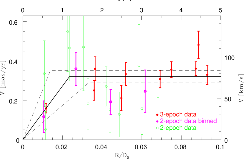
Figure 6.— The LMC rotation curve inferred from the observed PM field as described in Section 4.5.1. $V$ is the rotation velocity in the disk at cylindrical radius $R$. The left and bottom axes are expressed in angular and dimensionless units, respectively, as directly constrained by the data. The right and top axes show the corresponding physical units, assuming an LMC distance $D_{0}=50.1\>{\rm kpc}$ ($m-M=18.50$). Green and red data points show the results from individual HST fields with two and three epochs of data, respectively. Magenta data points show the result of binning the two-epoch data points into $R/D_{0}$ bins of size $0.018$. The red and magenta data points are listed in Table 3. The black curve is the best-fit parameterization of the form given by equation (2), with the surrounding black dashed curves indicating the $1\sigma$ uncertainty.

P08 estimated the PM rotation curve from only the two-epoch PM data. Their rotation velocity amplitude $V_{0,{\rm PM}}=120\pm 15\ {\rm{km\ s^{-1}}}\>$ was surprisingly high. This exceeds the value derived from the radial velocities of HI and young stars by approximately 30–$40\ {\rm{km\ s^{-1}}}\>$ (O11). It would be hard to understand how any stars in the LMC could be rotating significantly faster than the HI gas. When we use the method discussed above on our own reanalysis of the two-epoch PM data, the resulting unparameterized rotation curve is qualitatively similar to that of P08, but the uncertainties are very large. With the improved quality of our three-epoch data, the rotation curve is much better determined. Moreover, the rotation amplitude comes down to $V_{0,{\rm PM}}=76.1\pm 7.6\ {\rm{km\ s^{-1}}}\>$. This is more in line with expectation, and removes a significant puzzle from the previous work.

The uncertainties in our unparameterized rotation curve in Table 3 are underestimates, because they do not take into account the propagated uncertainties in other model parameters (such as the dynamical center, viewing angles, and COM motion). The weighted average $V/D_{0}$ in Table 3 for $R>R_{0}$ equals $0.323\pm 0.015$ mas/yr. By contrast, the best-fit from the parameterized model in Table 1 is $0.320\pm 0.029$ mas/yr. Since errors add in quadrature, the uncertainties in the other model parameters contribute an uncertainty of $0.025$ mas/yr to the rotation amplitude. This dominates the error budget, even though it is small compared to the typical per-field error bars in Table 3. So the per-field PM uncertainties are not the main limiting factor in our understanding of the rotation curve amplitude.

When we fit not only the PM data, but also the LOS velocity data, then the PM rotation amplitude $V_{0,{\rm PM}}$ changes by about the random uncertainty $\Delta V_{0,{\rm PM}}=\pm 7.6\ {\rm{km\ s^{-1}}}\>$. When we fit the old star $v_{\rm LOS}$ sample, $V_{0,{\rm PM}}$ goes up, and when we fit the young star sample, $V_{0,{\rm PM}}$ goes down. This is because the inclusion of the LOS velocities alters the best-fit line-of-nodes position angle $\Theta$ to lower or higher values, respectively (Table 1). This affects $V_{0,{\rm PM}}$, because our Monte-Carlo simulations show that $\Theta$ is anti-correlated with $V_{0}$.

4.5.2 Rotation Curve from the Line of Sight Velocity Field

In our best-fit models to the $v_{\rm LOS}$ data (combined with the PM data), the rotation amplitude $V_{0,{\rm LOS}}$ is not very accurately determined. This is because only a fraction $\sin i$ of any velocity is observed along the line of sight. The inclination is not accurately known from our or any other data (see Section 4.2), and the deprojection therefore introduces significant uncertainty. By contrast, $V_{0,{\rm LOS}}\>\sin i$ is determined much more accurately. For our old star sample, we find that $V_{0,{\rm LOS}}\>\sin i=30.9\pm 2.6\ {\rm{km\ s^{-1}}}\>$. This is consistent with the result from vdM02 (see Table 2). For our young star sample, we find that $V_{0,{\rm LOS}}\>\sin i=39.4\pm 1.9\ {\rm{km\ s^{-1}}}\>$. So the young stars have a higher rotation curve amplitude than the old stars, consistent with previous findings. However, the value inferred here is about 20% less than the value implied by the rotation curve fits of O11, for the same sample of stars (but not including PMs). This is due primarily to the larger value of $\Theta$ inferred here.

As for the PM case, we also determined unparameterized rotation curves from the LOS velocity data, separately for the young and old star samples. For this we kept all model parameters fixed, except the rotation amplitude, to the values in Table 1. We then binned the stars by their radius $R^{\prime}=R/D_{0}$ in the disk, and fit the rotation amplitude separately for each radial bin. The rotation curves thus obtained are listed in Table 4. The uncertainties only take into account the shot noise from the finite number of stars. This yields underestimates, because it does not take into account the propagated uncertainties in other model parameters. The inferred rotation curves are shown in Figure 7, together with the parametrized fits from Table 1. The rotation curves are well fit by the simple parameterization given by equation (2). For the parameterized fits, the uncertainty in the amplitude shown is $(\Delta V_{0,{\rm LOS}}\>\sin i)/\sin i$; so this includes the propagated uncertainty from all model parameters except the inclination. In general, for all rotation curve results derived here from LOS velocities, the inclination is the dominant uncertainty ($\Delta V/V=[\Delta i/180^{\circ}]\pi/\tan i$).

The turnover radii in our rotation curve fits, $R_{0}/D_{0}=0.075\pm 0.006$ for the old stars, and $R_{0}/D_{0}=0.040\pm 0.004$ for the young stars, are similar to what was found by vdM02 and O11, respectively (Table 2). The value of $R_{0}$ for the young stars is only about half that for the old stars. So the young stars not only have a higher rotation curve amplitude, but the rotation curve also rises faster. The value of the turnover radius $R_{0}/D_{0}$ inferred from the fit to only the PM data, $R_{0}/D_{0}=0.024\pm 0.010$, is even lower than the value for the young star $v_{\rm LOS}$ sample, but only at the $\sim 1.5\sigma$ level. We do not attach much significance to this, given the sparse radial sampling of our PM data, especially with high-quality WFC3 fields at small radii (only one field at $R<2.5$ kpc; see Figure 7). The radial behavior and turnover of the rotation curve are therefore more reliably constrained by the LOS data than by the PM data.

The values of $V_{0,{\rm LOS}}$ implied by our fits are $55.2\pm 10.3$ for the old stars, and $89.3\pm 18.8$ for the young stars, respectively. These results are consistent with the results obtained by vdM02 and O11 (Table 2). It should be noted that while O11 reported $V_{0,{\rm LOS}}=87\pm 5\ {\rm{km\ s^{-1}}}\>$ for the same sample of young stars, their listed uncertainty did not include the uncertainty from propagation of uncertainties in the center, inclination, COM PM, or distance. The inclination alone (from vdMC01, as adopted by O11) adds a $14\ {\rm{km\ s^{-1}}}\>$ uncertainty. So while the random uncertainties between our fit and that of O11 are in fact similar, our result should be more accurate in a systematic sense. This is because of our new determination of, e.g., the dynamical center and the COM PM. The good agreement between the $V_{0,{\rm LOS}}$ values reported here and in O11 is actually somewhat fortuitous. We find the LOS component of the rotation to be $\sim 20$% less than O11 did, but they adopted a larger inclination.

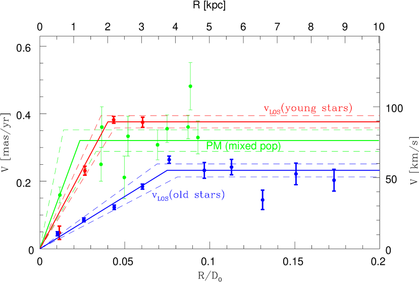
Figure 7.— Comparison of LMC rotation curves inferred from different tracers as described in the text, with axes similar to Figure 6. Red/Blue: young/old star $v_{\rm LOS}$ sample from Table 4; Green: three-epoch HST PM data from Table 3. Solid curves are the best-fit parameterizations of the form given by equation (2), with parameters from Table 1. The surrounding dashed curves indicate the $1\sigma$ uncertainty. Errorbars on the data points include only the shot/random noise from the measurements. The parameterized curves also include the propagated errors from the uncertainties in other LMC model parameters, except that the $v_{\rm LOS}$ fits shown do not include the inclination uncertainties.

4.5.3 Comparison of Proper Motion and Line of Sight Rotation Curves

The rotation amplitude inferred from our PM data, $V_{0,{\rm PM}}=76.1\pm 7.6\ {\rm{km\ s^{-1}}}\>$, falls between the values inferred from the LOS velocities of old stars, $V_{0,{\rm LOS}}=55.2\pm 10.3\ {\rm{km\ s^{-1}}}\>$, and young stars, $V_{0,{\rm LOS}}=89.3\pm 18.8\ {\rm{km\ s^{-1}}}\>$, respectively (see also Figure 7). This is because our stellar PM sample is essentially a magnitude limited sample, composed of a mix of young and old stars.

To assess quantitatively whether the rotation amplitudes derived from the PM data and LOS velocities are consistent, let us assume that a fraction $f$ of the stars that contribute to our PM measurements are young, and a fraction $(1-f)$ are old. The designations “young” and “old” in this context refer to the fact that the stars are assumed to have the same kinematics as the stars in our young and old $v_{\rm LOS}$ samples. This implies an expected PM-inferred rotation amplitude $V_{0,{\rm PM}}=55.2+f(34.1)\pm\sqrt{(}[(1-f)10.3]^{2}+[f18.8]^{2})\ {\rm{km\ s^{-1}}}\>$. Equating this with the observed $V_{0,{\rm PM}}$ implies that $f=0.61\pm 0.42$.

Table 4LMC rotation curve from LOS velocities

$R/D_{0}$	$R$	$V$	$\Delta V$	$V$	$\Delta V$
		[young]	[young]	[old]	[old]
	(kpc)	(km/s)	(km/s)	(km/s)	(km/s)
(1)	(2)	(3)	(4)	(5)	(6)
0.011	0.5	11.2	4.7	10.6	1.4
0.026	1.3	54.9	3.1	20.3	1.4
0.044	2.2	90.7	2.4	29.2	1.6
0.060	3.0	89.0	3.6	43.7	1.7
0.076	3.8	$\ldots$	$\ldots$	62.7	2.5
0.097	4.9	$\ldots$	$\ldots$	55.2	5.5
0.113	5.7	$\ldots$	$\ldots$	57.4	5.4
0.131	6.6	$\ldots$	$\ldots$	34.4	6.8
0.151	7.6	$\ldots$	$\ldots$	52.7	7.6
0.173	8.7	$\ldots$	$\ldots$	48.3	7.6

Note. — Column (1) lists $R^{\prime}\equiv R/D_{0}$, where $R$ is the radius in the disk. Column (2) lists the corresponding $R$ in kpc, for an assumed LMC distance $D_{0}=50.1\>{\rm kpc}$ ($m-M=18.50$). Columns (3) and (4) list the rotation velocity $V$ in km/s with its uncertainty, determined as in Section 4.5.2, for the young $v_{\rm LOS}$ sample. Columns (5) and (6) list the same quantities for the old $v_{\rm LOS}$ sample. Error bars include only the shot noise from the measurements, and not the propagated errors from the uncertainties in other LMC model parameters. The rotation curves are shown in Figure 7.

Figure 6 of K06 shows a color-magnitude diagram (CMD) of the LMC stars that contribute to our PM measurements. At the magnitudes of interest, there are two main features in this diagram. There is a blue plume, consisting of main sequence stars and evolved massive stars at the blue edge of their blue loops. And there is a red plume, consisting mostly of RGB stars and some AGB stars. Bright RSGs, such as those in the $v_{\rm LOS}$ samples, are too rare to contribute significantly to our small HST fields. To count the relative numbers of blue and red stars, we adopt a separation at $V-I=0.65$. We then find that the fraction of blue stars (as ratio of the total stars that contribute to our PM measurements) increases from $\sim 50$% at the brightest magnitudes to $\sim 70$% at the faintest magnitudes. If we assume that the blue stars have kinematics typical of young stars, and the red stars have kinematics typical of old stars, then this implies $f\approx 0.6\pm 0.1$. This CMD-based value is in excellent agreement with the value inferred above from the observed kinematics. So to within the uncertainties, the observed rotation of the LMC in the PM direction is consistent with the observed rotation in the LOS direction.

The LMC rotation amplitude $V_{0,{\rm PM}}$ inferred from the PM field is relatively insensitive to the inclination (see Section 2.3). By contrast, the LOS velocity data accurately constrain $V_{0,{\rm LOS}}\>\sin i$. Since the fraction $f$ must be between 0 and 1, comparison of these quantities can set limits on the inclination. The inclination must be such that $[V_{0,{\rm LOS}}\>\sin i]_{\rm old}/\sin i\leq V_{0,{\rm PM}}\leq[V_{0,{\rm LOS}}\>\sin i]_{\rm young}/\sin i$. With the inferred values from Table 1 this implies that at $1\sigma$ confidence $18.5^{\circ}\leq i\leq 39.3^{\circ}$. As discussed in Section 4.2, this encompasses most of the results reported in the literature. Alternatively, we could be less conservative and assume that we know from the CMD analysis that $f=0.6\pm 0.1$. In that case we obtain the more stringent range $24.3^{\circ}\leq i\leq 32.4^{\circ}$. But this assumes that we know the difference in kinematics between different stars in our HST CMDs, which has not actually been measured.

4.6. Kinematical Distance Estimates

So far, we have assumed that the distance $D_{0}$ to the LMC center of mass is known. However, a comparison of the PM and LOS velocity fields does in fact constrain the distance independently, since PMs are measured in mas/yr, and LOS velocities are measured in km/s. As we will discuss, this comparison provides several independent distance constraints.

The first distance constraint is obtained by requiring that the rotation amplitude measured from PMs matches that obtained from LOS velocities. This is called the “rotational parallax” method. Based on the discussion in the previous section, this implies that

$$D_{0}=(f[V_{0,{\rm LOS}}]_{\rm young}+(1-f)[V_{0,{\rm LOS}}]_{\rm old})/[V_{0,{\rm PM}}/D_{0}].$$ (6)

To use this equation, we must assume the relative fractions of young and old stars that contribute to the PM measurements. Using the analysis in Section 4.5.3, we set $f=0.6\pm 0.1$. With the inferred values from Table 1 this implies that $D_{0}=18.48\pm 0.40$. This is consistent with existing knowledge (e.g., Freedman et al. 2001). However, the uncertainty is very large, due primarily to the uncertainties in the LMC inclination. To obtain a distance estimate with a random error $\Delta(m-M)\leq 0.1$, the inclination would have to be known to better than $1.5^{\circ}$, not even accounting for other uncertainties. Based on the discussion in Section 4.2, it is clear that this is not currently the case, despite many papers devoted to the subject. Moreover, one would need to know the fraction $f$ more accurately than is possible with only CMD information. So for the LMC, the method of rotational parallax is not likely to soon yield a competitive distance estimate.

An alternative method to constrain the LMC distance from comparison of the PM and LOS velocity fields uses the observed LOS velocities perpendicular to the line of nodes. Rotation is perpendicular to the line of sight there, so that the observed velocities are due entirely to the solid-body rotation induced by the LMC’s transverse motion. Hence, the velocities obey $v_{\rm LOS}=\pm D_{0}\mu_{\perp}\sin\rho$, where $\rho$ is the distance from the COM, and $\mu_{\perp}$ is the component of the COM PM that lies along the line of nodes (vdM02). Since $\mu_{\perp}$ is constrained by the PM data in mas/yr, the distance $D_{0}$ can be determined from the LOS data in km/s. For accurate results, this method benefits from having data that extends to large distances $\rho$, and from having a sample with many velocity measurements. We therefore apply it to the old star $v_{\rm LOS}$ sample (see Figure 4). To use the full information content of the data, and to adequately propagate all uncertainties, one must fit the combined PM and old star $v_{\rm LOS}$ sample with $m-M$ as a free parameter. When we do this while keeping $\Theta=139.1^{\circ}\pm 4.1^{\circ}$ fixed to the previously obtained value from Table 1, we obtain $m-M=18.53\pm 0.20$ (similar to an earlier estimate in van der Marel et al. (2009), which was based on the vdM02 carbon star LOS velocity data and the K06 COM PM estimate). This has a smaller random error than the result from the rotational parallax method, but is still not competitive with existing knowledge. Moreover, it may be a biased estimate. When fitting $m-M$, one should really fit $\Theta$ simultaneously, because $\Theta$ and $m-M$ are generally anti-correlated in our model fits. However, we found that the multi-dimensional solution space becomes more degenerate when both $\Theta$ and $m-M$ are left to vary. Specifically, the best fit $m-M$ can vary by $\pm 0.2$, depending on how we choose to weight the PM data relative to the LOS velocity data in the $\chi^{2}$ definition (eq. [4]). So this method does not currently yield a competitive distance either.

A final method for estimating the the LMC distance from comparison of the PM and LOS velocity fields uses the observed systemic LOS velocity. As stated in Section 4.4, our PM field fit constrains $v_{\rm LOS,0}/D_{0}=1.675\pm 0.687$ mas/yr. Using the known systemic LOS velocity $v_{\rm LOS,0}=261.1\pm 2.2\ {\rm{km\ s^{-1}}}\>$ for the old star $v_{\rm LOS}$ sample, this yields an estimate for the distance: $m-M=17.58\pm 0.89$. Again, this is consistent with existing knowledge, but not competitive in terms of accuracy.

4.7. Disk Precession and Nutation

The preceding analysis in this paper has assumed that the viewing angles of the LMC disk are constant with time. vdM02 showed that there are additional contributions to PM and LOS velocity fields when the viewing angles vary with time, i.e., $di/dt\not=0$ or $d\Theta/dt\not=0$. This corresponds to a precession or nutation of the spin axis of the LMC disk. To induce such motion requires external tidal torques. While it is not impossible that such motion may exist, there is no theoretical requirement that it should.

The main impact of a value $di/dt\not=0$ is to induce a solid-body rotation component in the LOS velocity field, with its steepest gradient perpendicular to the line of nodes. To assess the existence of such a component, we repeated our fits to the combined PM data and old star $v_{\rm LOS}$ sample, but now with $di/dt$ free to vary. This yields $di/dt=-0.08\pm 0.17$ mas/yr. This result is consistent with zero. So with the presently available data, there is no need to invoke a non-zero value of $di/dt$.

Constraints on $di/dt$ from the young star $v_{\rm LOS}$ sample are weaker, because those data don’t extended as far from the COM, and don’t have as many velocity measurements. O11 inferred $di/dt=-0.66\pm 0.29$ mas/yr for that same sample ($-184^{\circ}\pm 81^{\circ}$ Gyr^-1). However, their uncertainty is an underestimate, because it does not propagate the known uncertainties in the center, inclination, COM PM, or distance. Based on our analysis of the young stars, we have found no compelling reason to assume they require $di/dt\not=0$. It would in fact be difficult to understand how the spin axis of the young star disk could be moving relative to the old star disk.

A value $d\Theta/dt\not=0$ does not affect the LOS velocity field. However, it does cause circular motion in the observed PM field. This is almost entirely degenerate with the actual rotation of the LMC disk, as measured by the rotation amplitude $V_{0,{\rm PM}}$ (compare Figure 2). We have shown in Section 4.5.3 that the amplitude inferred assuming $d\Theta/dt=0$ agrees with the rotation amplitudes inferred from LOS velocities. Therefore, the data do not require a value $d\Theta/dt\not=0$. If there is a deviation from zero, it would have to be small enough to not perturb the agreement discussed in Section 4.5.3.

4.8. Mass

To estimate the dynamical mass of the LMC, it is necessary to know the kinematics of tracers at large radii. The outermost tracers for which kinematics are available are the old stars in our $V_{\rm LOS}$ sample (see Figure 4), most of which are carbon stars from Kunkel et al. (1997; see Figure 3). Figure 7 shows that the rotation curve of these stars stays more-or-less flat out the last data point, at radius $R=8.7\>{\rm kpc}$ in the disk (see also figure 6 of vdM02). Since this is true for the old stars, it must be true for the young stars as well. After all, both orbit in the same gravitational potential.

Based on this reasoning, we infer that the young stars have a rotation amplitude $V_{0,{\rm LOS}}=89.3\pm 18.8\ {\rm{km\ s^{-1}}}\>$ at $R=8.7\>{\rm kpc}$. Olsen & Massey (2007) inferred a velocity dispersion for these stars of $\sigma_{\rm LOS}=9\ {\rm{km\ s^{-1}}}\>$. The formalism of vdM02 then implies an upward asymmetric drift correction of only $\Delta V=2.4\ {\rm{km\ s^{-1}}}\>$, much smaller than the random errors. This is as expected, given that O11 found that the young stars and HI gas have essentially the same rotation curve. So we obtain that $V_{\rm circ}=91.7\pm 18.8\ {\rm{km\ s^{-1}}}\>$ at $R=8.7$ kpc, with the error dominated by inclination uncertainties.

The total mass of the LMC inside the last measured data point is $M_{\rm LMC}(R)=RV_{\rm circ}^{2}/G$, where the gravitational constant $G=4.3007\times 10^{-6}\>{\rm kpc}(\ {\rm{km\ s^{-1}}}\>)^{2}\>{\rm M_{\odot}}^{-1}$. This yields $M_{\rm LMC}(8.7\>{\rm kpc})=(1.7\pm 0.7)\times 10^{10}\>{\rm M_{\odot}}$. This is consistent with the total mass of the LMC that has been used in several past $N$-body simulation studies of the LMC (e.g., Gardiner & Noguchi 1996). However, this is likely an underestimate of the total LMC mass. Since the rotation curve is flat, the mass likely continues to rise almost linearly beyond $8.7\>{\rm kpc}$. Many virial masses are possible, as long as the concentration of the dark halo is varied to reproduce the dynamical mass. In Paper I we considered models with virial masses up to $25\times 10^{10}\>{\rm M_{\odot}}$.

4.9. Tidal Radius

The tidal radius of the LMC can be estimated using the formalism of vdM02. We assume that the LMC rotation curve is flat at $V_{\rm circ}=91.7\pm 18.8\ {\rm{km\ s^{-1}}}\>$, and the Milky Way rotation curve at the distance of the LMC is flat at $V_{\rm MW}=206\pm 23\ {\rm{km\ s^{-1}}}\>$ (based on the enclosed mass out to the LMC distance given by Kochanek 1996). This implies a tidal radius of $22.3\pm 5.2\>{\rm kpc}$ (i.e., a radius on the sky of $24.0^{\circ}\pm 5.6^{\circ}$). If instead there is no LMC mass outside of $8.7\>{\rm kpc}$, then the tidal radius is smaller by a factor $0.73$. Either way, the LMC tidal radius is beyond $17^{\circ}$. Indeed, photometric studies of the LMC have traced the LMC disk almost this far out (Saha et al. 2010).

4.10. Tully-Fisher Relation

To determine whether the rotation curve of the LMC is typical, it is useful to assess how its circular velocity compares to that of other similar galaxies. The classical Tully-Fisher relation in spirals has been shown to extend into the low-mass regime when the total baryonic content of the galaxies is used (gas in addition to stars; McGaugh et al. 2005; Stark et al. 2009). In Figure 8 (blue triangle) we place the LMC on the baryonic Tully-Fisher (BTF), using $V_{\rm circ}$ from Section 4.8 and $M_{\rm b}=3.2\times 10^{9}\>{\rm M_{\odot}}$ from vdM02.

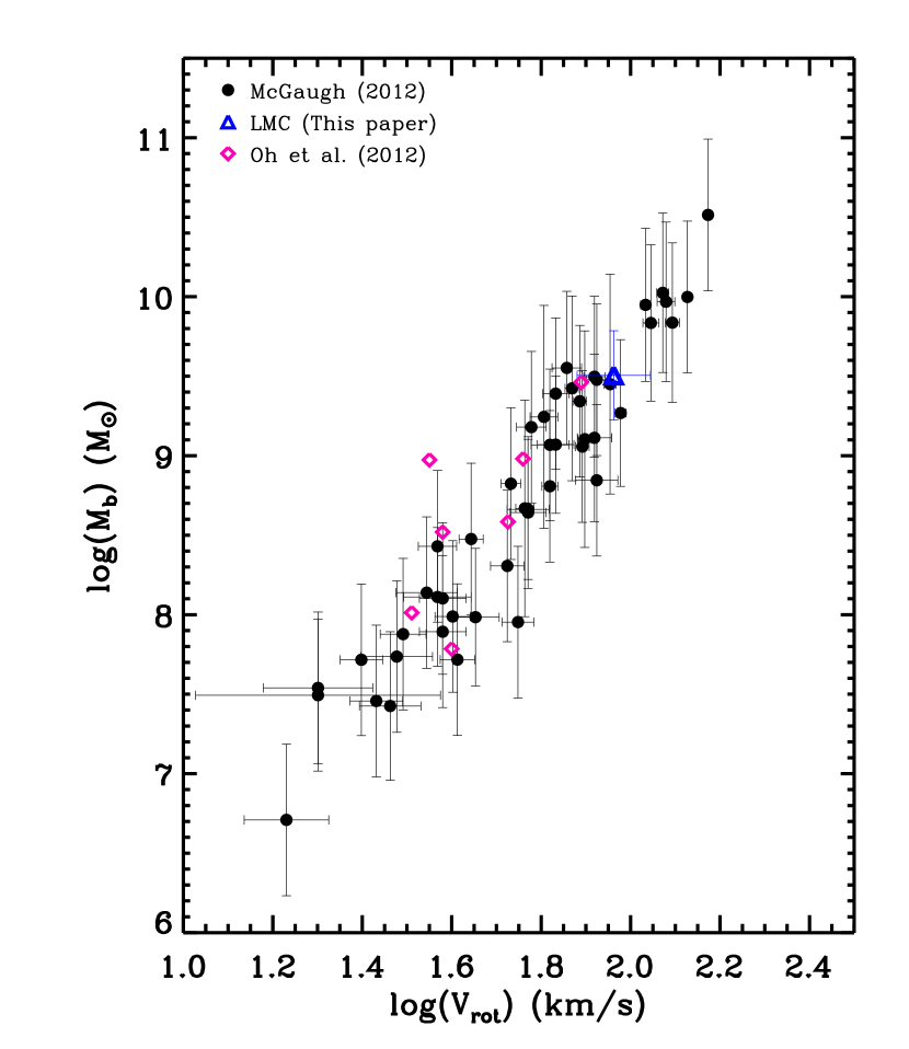
Figure 8.— Baryonic galaxy mass versus rotation velocity in a log-log plot. The LMC (blue triangle) follows the baryonic Tully-Fisher relation defined by low-mass gas-dominated galaxies (black circles; McGaugh 2012) and dwarf galaxies from the THINGS survey (pink diamonds; Oh et al. 2012a,b).

McGaugh (2012) recently calibrated the BTF relation using a sample of gas-dominated low-mass systems, arguing that the errors introduced by modeling the stellar component is minimized in these gas-rich systems. These galaxies follow a very tight relation. As with high-mass galaxies, the scatter is below what is expected from initial conditions in cosmological models, implying the need for some feedback process that is correlated with the galaxy potential (Eisenstein & Loeb 1996; McGaugh 2012). Similarly, Oh et al. (2011a) placed a sample of dwarf galaxies from the HI Nearby Galaxy Survey (THINGS; Walter et al. 2008), a high velocity-resolution HI survey of dwarf galaxies, on the BTF relation. In Figure 8, black points show gas-rich low-mass galaxies compiled in McGaugh (2012) and pink diamonds show the THINGS dwarfs from Oh et al. (2011a,b). The LMC falls on the BTF relation followed by these galaxies. So even though the LMC is a member of an interacting pair, it is not atypical in terms of its BTF position.

As discussed in Section 4.8, the error in our $V_{\rm circ}$ is dominated by inclination uncertainties. So if one assumes a priori that the LMC must fall exactly on the BTF, then this would in principle provide an alternative method to constrain the LMC inclination (see also Oh et al. 2011a). Also, central density profile slopes are a powerful probe of the properties of dark matter (Navarro, Frenk, & White et al. 1997; Dalcanton & Hogan 2001), and these can be constrained from observed rotation curves of dwarf galaxies (e.g., de Blok 2010, and references therein; Oh et al. 2011a,b). However, for the LMC only sparse discrete PM and LOS datasets are available, and these are not ideally suited for constraining the central rotation curve slope. Also, the possibility of non-circular orbits in the poorly understood LMC bar region would complicate any interpretation. So we have decided not to pursue a detailed rotation curve decomposition here.

5. Conclusions

We have presented a detailed study of the large-scale rotation of the LMC based on observed stellar velocities in all three Cartesian directions. This is the first time that such a study has been possible for any galaxy, made possible by the exquisite capabilities of HST for measuring PMs in the nearby Universe. While the LOS velocity field of the LMC has been studied previously using many tracers, our analysis of the PM rotation field is new. This is important, because the PM rotation field is defined by two components of motion, and it therefore has a higher information content than the LOS velocity field. As a result, quantities that are degenerate in analyses of the LOS velocity field (such as the rotation curve, the inclination, and one component of the transverse motion of the COM) are uniquely determined by analysis of the PM rotation field. We interpret the data with simple models of circular rotation in a flat disk, which fit the data reasonably well. By and large, we find that the LMC rotation properties as revealed by PM and LOS data are mutually consistent, as they should be. However, by analyzing accurate PM data and combining it with existing LOS data we do obtain several new insights into the geometry, kinematics, and structure of the LMC.

Previous studies of the LMC have found that the photometric center is offset significantly from the dynamical center defined by the rotating HI gas disk. This is not difficult to explain, since the LMC has a lopsided off-center bar that could be a transient feature induced by the LMC’s interaction with the SMC. What is more puzzling has been the finding that the LOS velocity field of stellar tracers is best fit by a dynamical center that is also offset from the HI dynamical center. Our new analysis of the PM rotation field does not confirm this. We find that the stellar dynamical center revealed by PMs agrees with the HI dynamical center. However, we also find that previous analyses of the LOS velocity field were not in error. Our new analysis of the now very large sample of available LOS velocity data continues to indicate a dynamical center offset, albeit by a smaller amount than reported previously. This cannot be real, since the PM and LOS analyses observe the same stellar populations. This likely reveals limitations of the simple rotation model used. In reality, the stars and gas in the LMC probably do have the same dynamical center, because they orbit in the same gravitational potential.

The best-fit values for the viewing angles that define the orientation of the LMC disk, as inferred from the PM rotation field, are within the range of values implied by previous studies. However, several puzzles remain. First, the position angle of the line of nodes $\Theta$ is not the same for the young and old stellar populations of the LMC. When LOS velocities of the young population are fit jointly with the PM data, we obtain $\Theta=154.5^{\circ}\pm 2.1^{\circ}$. By contrast, when LOS velocities of the old population are fit jointly with the PM data, we obtain $\Theta=139.1^{\circ}\pm 4.1^{\circ}$. When the PM data are fit by themselves, the intermediate result $\Theta=147.4^{\circ}\pm 10.0^{\circ}$ is obtained. The second puzzle is that all these kinematically determined values are larger than several results obtained from geometrical methods (e.g., vdMC01, Rubele et al. 2012). Similarly for the inclination, the results obtained here and those discussed in the literature span a much larger range than the random errors in the individual measurements. These results can be explained if the structure of the LMC is more complicated than a single flat disk in circular rotation. Indeed, the data provide indications for variations with both stellar population and radius in the disk. However, by contrast to previous authors we have found no evidence for precession or nutation of the LMC disk. Given the latest insights into the position and motion of the LMC COM, we find that acceptable fits to all the kinematical data can be obtained with $di/dt=0$ and $d\Theta/dt=0$.

The LMC rotation curve as implied by our PM measurements has an amplitude $V_{0,{\rm PM}}=76.1\pm 7.6\ {\rm{km\ s^{-1}}}\>$. This applies to a magnitude-limited sample, composed of a mix of stellar populations. This value of $V_{0,{\rm PM}}$ falls between the rotation amplitudes implied by the LOS velocities of old and young stars, $V_{0,{\rm LOS}}=55.2\pm 10.3$ and $89.3\pm 18.8$, respectively. These results are quantitatively consistent with the natural hypothesis that the blue stars in our HST CMDs have predominantly young-star kinematics and the red stars have predominantly old-star kinematics. These results resolve a puzzle posed by analysis of the two-epoch PM rotation curve amplitude. P08 previously reported $V_{0,{\rm PM}}=120\pm 15\ {\rm{km\ s^{-1}}}\>$, which was difficult to understand as it exceeded the rotation amplitude of both the young stars and the HI gas.

After correction for asymmetric drift, we infer a circular velocity for the LMC of $V_{\rm circ}=91.7\pm 18.8\ {\rm{km\ s^{-1}}}\>$. The large uncertainty is due mostly to uncertainties in the inclination of the LMC. This $V_{\rm circ}$ places the LMC on the same baryonic Tully-Fisher relation defined by samples of other low-mass gas-rich galaxies. Also, it implies an enclosed mass $M_{\rm LMC}=(1.7\pm 0.7)\times 10^{10}\>{\rm M_{\odot}}$, out to the radius $8.7\>{\rm kpc}$ to which it has been verified that the rotation curve remains approximately flat. The virial mass of the LMC should be larger than this, with the exact value depending on how far the LMC’s dark halo extends, and on whether it has been tidally truncated. If the LMC circular velocity curve remains flat outside of the region probed observationally, then the tidal radius is $22.3\pm 5.2\>{\rm kpc}$ (i.e., a radius on the sky of $24.0^{\circ}\pm 5.6^{\circ}$).

We have discussed three independent methods for combining PM and LOS velocity information to obtain a kinematical estimate for the LMC distance. While each of these methods yields results that are consistent with existing knowledge, none of them is currently competitive in terms of accuracy. This is due in large part to the fact that the exact viewing angles of the LMC continue to be poorly understood. These distance determination methods might become competitive in the future, if better PM data become available and our understanding of the structure and orientation of the LMC improve further.

References

- (1)
- (2) Bekki, K. 2009, MNRAS, 393, L60
- (3)
- (4) Bekki, K. 2011, ApJ, 730, L2
- (5)
- (6) Besla, G., Kallivayalil, N, Hernquist, L., Robertson, B., Cox, T. J., van der Marel, R. P., & Alcock, C. 2007, 668, 949
- (7)
- (8) Besla, G., Kallivayalil, N., Hernquist, L., van der Marel, R. P., Cox, T. J., Keres, D. 2012, MNRAS, 421, 2109
- (9)
- (10) Binney, J., & Merrifield, M. 1998, Galactic Astronomy, (Princeton: Princeton University Press)
- (11)
- (12) Binney, J., & Tremaine, S. 1987, Galactic Dynamics, 2nd ed. (Princeton: Princeton University Press)
- (13)
- (14) Borissova, J., Minniti, D., Rejkuba, M., & Alves, D. 2006, A&A, 460, 459
- (15)
- (16) Boylan-Kolchin, M., Bullock, J. S., Sohn, S. T., Besla, G., & van der Marel, R. P. 2013, ApJ, 768, 140
- (17)
- (18) Brunthaler, A., Reid, M. J., Falcke, H., Greenhill, L. J., & Henkel, C. 2005, Science, 307, 1440
- (19)
- (20) Brunthaler, A., Henkel, C., de Blok, W. J. G., Reid, M. J., Greenhill, L. J., & Falcke, H. 2006, A&A, 457, 109
- (21)
- (22) Brunthaler, A., Reid, M. J., Falcke, H., Henkel, C., & Menten, K. M. 2007, A&A, 462, 101
- (23)
- (24) Carrera, R., Gallart, C., Aparicio, A., & Hardy, E. 2011, AJ, 142, 61
- (25)
- (26) Cole, A. A., Tolstoy, E., Gallagher, J. S., III, & Smecker-Hane, T. A. 2005, AJ, 129, 1465
- (27)
- (28) Dalcanton, J. J., Hogan, C. J. 2001, ApJ, 561, 35
- (29)
- (30) de Blok, W. J. G. 2010, Adv. Astron., 2010, 1
- (31)
- (32) de Vaucouleurs, G., & Freeman, K. C. 1972, Vistas in Astronomy, 14, 1, 163
- (33)
- (34) Eisenstein, D. J., & Loeb, A. 1996, ApJ, 459, 432
- (35)
- (36) Feitzinger, J. V., Schmidt-Kaler, T., & Isserstedt, J. 1977, A&A, 57, 265
- (37)
- (38) Freedman, W. L., et al. 2001, ApJ, 553, 47
- (39)
- (40) Freedman, W. L., Madore, B. F., Scowcroft, V., Burns, C., Monson, A., Persson, S. E., Seibert, M., Rigby, J. 2012, ApJ, 758, 24
- (41)
- (42) Gardiner, L. T., & Noguchi, 1996, MNRAS, 278, 191
- (43)
- (44) Gould, A. 2000, ApJ, 528, 156
- (45)
- (46) Grocholski, A. J., Cole, A. A., Sarajedini, A., Geisler, D., & Smith, V. V. 2006, AJ, 132, 1630
- (47)
- (48) Hardy, E., Alves, D. R., Graff, D. S., Suntzeff, N. B., & Schommer, R. A. 2001, Ap&SS, 277, 471
- (49)
- (50) Haschke, R., Grebel, E. K., & Duffau, S. 2012, AJ, 144, 106
- (51)
- (52) Herrnstein, J. R., Moran, J. M., Greenhill, L. J., Diamond, P. J., Inoue, M., Nakai, N., Miyoshi, M., Henkel, C., & Riess, A. 1999, Nature, 400, 539
- (53)
- (54) Kallivayalil, N., van der Marel, R. P., Alcock, C., Axelrod, T., Cook, K. H., Drake, A. J., & Geha, M. 2006a, ApJ, 638, 772 (K06)
- (55)
- (56) Kallivayalil, N., van der Marel, R. P., & Alcock, C. 2006b, ApJ, 652, 1213
- (57)
- (58) Kallivayalil, N., van der Marel, R. P., Besla, G., Anderson, J., & Alcock, C. 2013, ApJ, 764, 161 (Paper I)
- (59)
- (60) Kim, S., Staveley-Smith, L., Dopita, M. A., Freeman, K. C., Sault, R. J., Kesteven M. J., & McConnell, D. 1998, ApJ, 503, 674
- (61)
- (62) Kochanek, C. S. 1996, ApJ, 457, 228
- (63)
- (64) Koerwer, J. F. 2009, AJ, 138, 1
- (65)
- (66) Kunkel, W. E., Demers, S., Irwin, M. J., & Albert, L. 1997, ApJ, 488, L129
- (67)
- (68) Lépine, S., Koch, A., Rich, R. M., & Kuijken, K. 2011, ApJ, 741, 100
- (69)
- (70) Luks, T., & Rohlfs, K. 1992, A&A, 263, 41
- (71)
- (72) Massey, P., & Olsen, K. A. G., 2003, AJ, 126, 2867
- (73)
- (74) McGaugh, S. S., Schombert, J. M., Bothun, G. D., & de Blok, W. J. G. 2005, ApJ, 632, 859
- (75)
- (76) McGaugh, S. S. 2012, AJ, 143, 40
- (77)
- (78) Meatheringham, S. J., Dopita, M. A., Ford, H. C., & Webster, B. L. 1988, ApJ, 327, 651
- (79)
- (80) Minniti, D., Borissova, J., Rejkuba, M., Alves, D. R., Cook, K. H., & Freeman, K. C. 2003, Science, 301, 1508
- (81)
- (82) Mo, H., van den Bosch, F. C., & White, S. D. M. 2010, Galaxy Formation and Evolution (Cambridge: Cambridge University Press)
- (83)
- (84) Navarro, J., Frenk, C. S., White, S. 1997, ApJ, 490, 493
- (85)
- (86) Nikolaev, S., Drake, A.J., Keller, S. C., Cook, K. H., Dalal, N., Griest, K., Welch, D. L., & Kanbur, S. M. 2004, 601, 260
- (87)
- (88) Oh, S.-H., de Blok, W. J. G., Brinks, E., Walter, F., & Kennicutt, R. C., Jr. 2011a, AJ, 141, 193
- (89)
- (90) Oh, S.-H., Brook, C., Governato, F., et al. 2011b, AJ, 142, 24
- (91)
- (92) Olsen, K. A. G., & Salyk, C. 2002, AJ, 124, 2045
- (93)
- (94) Olsen, K. A. G., & Massey, P. 2007, ApJ, 656, L61O
- (95)
- (96) Olsen, K. A. G., Zaritsky, D., Blum, R. D., Boyer, M. L., & Gordon, K. D. 2011, ApJ, 737, 29O (O11)
- (97)
- (98) Piatek, S., Pryor, C., & Olszewski, E. W. 2008a, AJ, 135, 1024 (P08)
- (99)
- (100) Piatek, S., & Pryor, C. 2008b, in “A Giant Step: from Milli- to Micro-arcsecond Astrometry,” Proc. IAU Symposium, 248, 244
- (101)
- (102) Press, W. H., Teukolsky, S. A., Vetterling, W. T., & Flannery, B. P. 1992, Numerical Recipes (Cambridge: Cambridge University Press)
- (103)
- (104) Prevot, L., et al. 1985, A&AS, 62, 23
- (105)
- (106) Pryor, C., Piatek, S., & Olszewski, E. W. 2010, AJ, 139, 839
- (107)
- (108) Rubele, S., et al. 2012, A&A, 537, A106
- (109)
- (110) Schommer, R. A., Suntzeff, N. B., Olszewski, E. W., & Harris, H. C. 1992, AJ, 103, 447
- (111)
- (112) Sohn, S. T., Anderson, J., & van der Marel, R. P. 2012, ApJ, 753, 7
- (113)
- (114) Sohn, S. T., Besla, G., van der Marel, R. P., Boylan-Kolchin, M., Majewski, S. R., & Bullock, J. S. 2013, ApJ, 768, 139
- (115)
- (116) Stark, D. V., McGaugh, S. S., & Swaters, R. A. 2009, AJ, 139, 312
- (117)
- (118) Subramanian, S., Subramaniam, A. 2013, A&A, 552, 144
- (119)
- (120) van den Bergh, S. 2000, The Galaxies of the Local Group (Cambridge: Cambridge University Press)
- (121)
- (122) van der Marel, R. P. 2001, AJ, 122, 1827
- (123)
- (124) van der Marel, R. P., & Cioni, M. R. L. 2001, AJ, 122, 1807
- (125)
- (126) van der Marel, R. P., Alves, D. R., Hardy, E., & Suntzeff, N. B. 2002, AJ, 124, 2639 (vdM02)
- (127)
- (128) an Astrophysical Laboratory”, Proc. STScI Symposium, M. Livio, T. M. Brown., eds., 47 (Cambridge, UK: Cambridge University Press)
- (129)
- (130) van der Marel, R. P., Kallivayalil, N., & Besla, G. 2009, in “The Magellanic System: Stars, Gas, and Galaxies,” Proc. IAU Symposium 256, 81
- (131)
- (132) van der Marel, R. P., Fardal, M., Besla., G., Beaton, R., Sohn, S. T., Anderson, J., Brown, T., & Guhathakurta, P. 2012a, ApJ, 753, 8
- (133)
- (134) van der Marel, R. P., Besla, G., Cox, T. J., Sohn, S. T., & Anderson, J. 2012b, ApJ, 753, 9
- (135)
- (136) Westerlund, B. E. 1997, The Magellanic Clouds (Cambridge: Cambridge University Press)
- (137)
- (138) Zhao, H., Ibata, R. A., Lewis, G. F., & Irwin, M. J. 2003, MNRAS, 339, 701
- (139)