THE ANTICORRELATED NATURE OF THE PRIMARY AND SECONDARY ECLIPSE TIMING VARIATIONS FOR THE KEPLER CONTACT BINARIES

Abstract

We report on a study of eclipse timing variations in contact binary systems, using long-cadence lightcurves in the Kepler archive. As a first step, ‘observed minus calculated’ ($O-C$) curves were produced for both the primary and secondary eclipses of some 2000 Kepler binaries. We find $\sim$390 short-period binaries with $O-C$ curves that exhibit (i) random-walk like variations or quasi-periodicities, with typical amplitudes of $\pm$200-300 seconds, and (ii) anticorrelations between the primary and secondary eclipse timing variations. We present a detailed analysis and results for 32 of these binaries with orbital periods in the range of $0.35\pm 0.05$ days. The anticorrelations observed in their $O-C$ curves cannot be explained by a model involving mass transfer, which among other things requires implausibly high rates of $\sim$$0.01\,M_{\odot}{\rm yr}^{-1}$. We show that the anticorrelated behavior, the amplitude of the $O-C$ delays, and the overall random-walk like behavior can be explained by the presence of a starspot that is continuously visible around the orbit and slowly changes its longitude on timescales of weeks to months. The quasi-periods of $\sim$$50-200$ days observed in the $O-C$ curves suggest values for $k$, the coefficient of the latitude dependence of the stellar differential rotation, of $\sim$0.003$-$0.013.

1. Introduction

Contact binary stars occur relatively frequently among binaries (Rucinski 1998). A contact binary system consists of two dwarf stars, most often from the F, G, and K spectral classes, that are surrounded by a common convective envelope. The orbital period distribution peaks in the 8 to 12 hour range. Most systems, though not all, have orbital periods between 0.2 and 1.0 days (Maceroni & van’t Veer 1996; Paczyński et al. 2006). While the masses of the two component stars of a contact binary are typically unequal, the two stars usually have approximately equal surface temperatures due to the effects of mass and energy transfer between the components via a common convective envelope (Lucy 1968). The properties of the envelope, the energy transfer between the components, and the overall internal structure of the components have been investigated by many authors (see, e.g., Kähler 2002; Webbink 2003; Kähler 2004; Csizmadia & Klagyivik 2004; Li et al. 2004; Yakut & Eggleton 2005; Stepień & Gazeas 2012). Eclipsing contact binaries are often referred to as W UMa systems in honor of the prototype.

Some variable stars that were classified as contact binaries in earlier studies are now considered otherwise; their light curves are thought to merely mimic the light curves of true contact binaries. For example, while AW UMa is actually a semi-detached system with a material ring, it exhibits a light curve much like that of a contact binary (Pribulla & Rucinski 2008). This example and others demonstrate that it may be difficult to determine in practice whether a binary is a contact or a semi-detached system based only on a photometric time series.

Although contact binaries make up an important part of the Galactic stellar population, their formation and final-stage evolutionary states are still not clear (Paczyński et al. 2006; Eggleton 2006). Possible formation processes and evolutionary outcomes have recently been summarized by Eggleton (2012). Many, if not all, contact binaries may be members of triple star systems, which could drive the formation of these extremely close binaries through a combination of the Kozai mechanism and tidal friction (Robertson & Eggleton 1977; Kozai 1962; Kiseleva et al. 1998; Fabrycky & Tremaine 2007). It is also thought that rapidly rotating single stars may be formed from the coalescence of the components of contact binaries (Li et al. 2008; Gazeas & Stepień 2008). These open questions about the formation, evolution, and final state of contact binaries make them one of the most intriguing classes of objects in stellar astrophysics (Eggleton 2012).

Many contact binaries show signs of stellar activity, presumably because the component stars are rapid rotators with deep convective zones. Doppler imaging has revealed that some contact binaries are almost fully covered by rather irregular spot-like structures (AE Phe, Maceroni et al. 1994 and Barnes et al. 2004; YY Eri, Maceroni et al. 1994; VW Cep, Hendry & Mochnacki 2000; SW Lac, Senavci et al. 2011). Signs of high levels of coronal activity are often apparent; this helps explain why contact binaries can be relatively strong X-ray emitters (Geske et al. 2006). It may be noted that the first flare event which was simultaneously observed both in X-rays and at radio wavelengths from a star other than our Sun was from the contact binary VW Cephei (Vilhu et al. 1988). Ground based multicolor photometry demonstrated an H$\alpha$ excess in two contact binary systems that is thought to have a coronal origin, and to be related to the presence of dark spots on the photosphere (Csizmadia et al. 2006).

Several contact binaries exhibit night-to-night light curve variations which may be explained by fast spot evolution on orbital- (or even suborbital-) period timescales (Csizmadia et al. 2004). On the other hand, the eclipse timing variations of several contact binaries show quasi-periodic oscillations on a time-scale of $\sim$10 years, and those features were interpreted as indirect evidence of solar-like magnetic cycles (see e.g., Qian 2003; Awadalla et al. 2004; Borkovits et al. 2005; Pop & Vamos 2012). These results are in accord with the work of Lanza & Rodonó (1999), which concluded that the timescales for magnetic modulations are strongly and positively correlated with the orbital periods of the systems. This relation makes contact binaries excellent laboratories in which to investigate the temporal variations and evolution of stellar spots, in part because the timescales of the variations are shorter than in other types of binary and single stars. However, the shortest among these timescales can be problematic to study using ground-based observatories because they are comparable to the length of an Earth night.

Kalimeris et al. (2002) noted that the migration of starspots on the surface(s) of the constituent stars in short-period binaries, especially contact binaries, could affect measurements of eclipse times and thereby mimic changes in the orbital period. Kalimeris et al. (2002) also showed that the perturbations to the observed minus calculated ($O-C$) eclipse-time curves would generally have amplitudes smaller than $\sim$0.01 days, and could appear to be quasiperiodic on timescales of a few hundred days or so if the spot migration is related to differential rotation of the host star.

The planet-finding Kepler mission (Borucki et al. 2010; Koch et al. 2010; Caldwell et al. 2010) has observed more than 150,000 stars over the past four years. The monitoring of each star is nearly continuous, and the photometric precision is exquisitely high (Jenkins et al. 2010a; 2010b). These capabilities have led to the discovery of more than 2600 planet candidates (Batalha et al. 2013), and also of a comparable number of binary stars (Slawson et al. 2011; Matijevič et al. 2012). Some 850 of the Kepler binaries have been classified as contact, overcontact, or elliposidal light variable (‘ELV’) systems (Slawson et al. 2011; Matijevič et al. 2012).

In this work we report on a study of eclipse timing variations of binaries in archival Kepler data, with a particular focus on contact and overcontact binaries. In Section 2 we describe the data preparation, the estimation of the eclipse times, and the production of $O-C$ curves for each contact binary. In Sect. 3 we present the $O-C$ data for an illustrative selection of 32 contact binaries (out of the several hundred we found) which exhibit common interesting features including random-walk like, or quasi-periodic excursions in the $O-C$ behavior with amplitudes of $\sim$$\pm$ 300 sec, and a generally anticorrelated behavior in the $O-C$ curves for the primary and secondary eclipse minima or ellipsoidal-light-variation minima. In Sect. 4 we extend the work of Kalimeris et al. 2002 in order to explain some of these characteristics with a very simple model involving a cool (or hot) spot on one of the stars that drifts slowly around the star on timescales of weeks to months. We discuss the significance of our results in Sect. 5.

2. Data Analysis

2.1. Data Preparation

The present study is based on Kepler long-cadence (LC) lightcurves. To start, we retrieved the LC lightcurve files for Quarters 1 through Quarter 13 for all of the candidates in the latest Kepler eclipsing binary catalog (Slawson et al. 2011) that were available at the Multimission Archive at STScI (MAST). We used the lightcurves made with the PDC-MAP algorithm (Stumpe et al. 2012; Smith et al. 2012), which is intended to remove instrumental signatures from the flux time series while retaining the bulk of the astrophysical variations of each target. For each quarter, the flux series was normalized to its median value. Then, for each target, the results from all available quarters were concatenated together in a single file. We also checked our results using the SAP-MAP processed data set, and the results are unchanged.

The next step in the data processing was to apply a high-pass filter to each stitched light curve. A smoothed light curve was obtained by convolving the unsmoothed light curve with a boxcar function of duration equal to the known binary period. The smoothed light curve was then subtracted from the unsmoothed light curve. This procedure largely removes intensity components with frequencies below about half the binary frequency, while leaving largely intact temporal structures that are shorter than the binary period. Periodically-recurring features of the light curve are essentially unaffected.

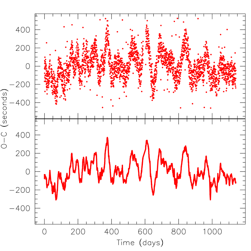
Figure 1.— Illustrative $O-C$ curve for one of the contact binaries considered in this work, KIC 2159783 (“KIC” refers to the Kepler Input Catalog; Batalha et al. 2010). Top panel: raw $O-C$ curve. Bottom panel: $O-C$ curve after performing a 5-day boxcar smoothing operation. The smoothed versions of the $O-C$ curves are the ones displayed in the remainder of this work.

2.2. $O-C$ Eclipse Times

Since long-cadence data with relatively coarse time resolution were used for the present study, an interpolation method was needed to estimate eclipse times with an accuracy better than $\sim$1700 s. The algorithm utilized for the determination of eclipse times consists simply of identifying the flux values in the light curve that represent local minima, and then fitting a parabola to that value and the immediately preceding and succeeding values. The time of the minimum of the fitted parabola is used as the time of eclipse minimum (see Rappaport et al. 2013 for details of the algorithm). This algorithm provides excellent accuracy for short-duration eclipses, but loses some accuracy when the eclipse duration is longer than $\sim$10 long-cadence samples. For contact binaries with periods between $\sim$0.2 and 1 day, however, the algorithm works well and typically yields eclipse times subject to an rms scatter of $\sim$30 s.

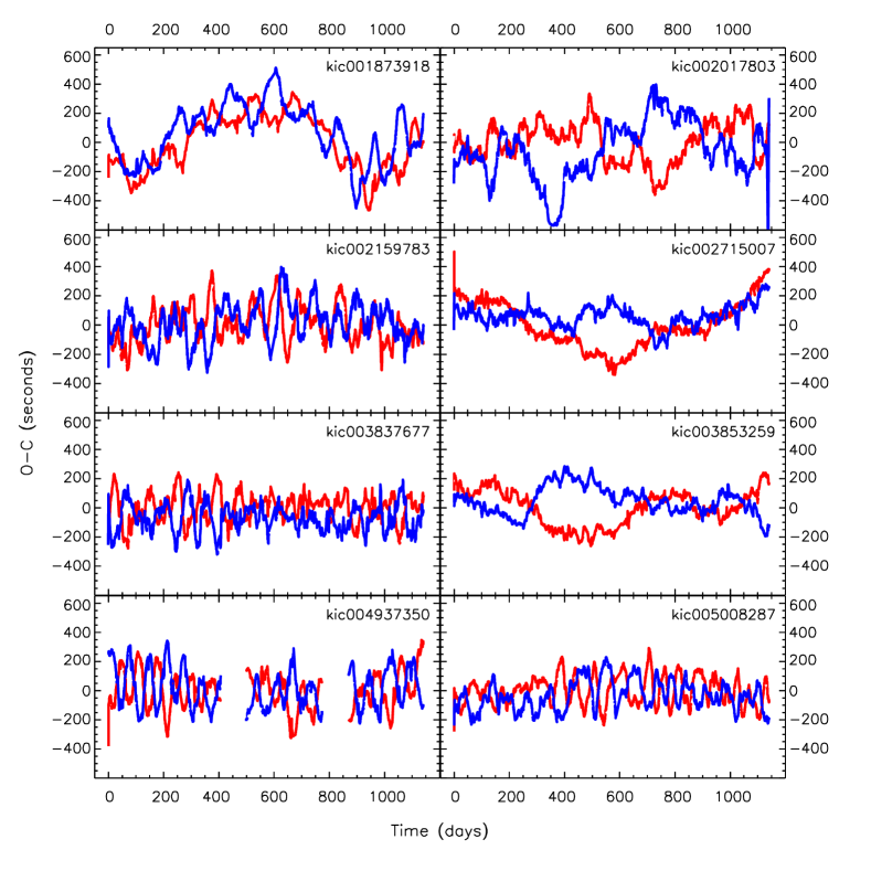
Figure 2.— A sample of $O-C$ curves for an illustrative set of eight Kepler contact binary systems with KIC numbers in the range of 1873918 to 5008287. The $O-C$ curves for the primary and secondary eclipses are shown as red and blue curves, respectively. The curves have been smoothed over a 5-day interval, comprising typically 10-15 eclipses. These $O-C$ curves typically exhibit random-walk-like or quasi-periodic behavior. The $O-C$ curves for the primary and secondary eclipses are often anticorrelated.

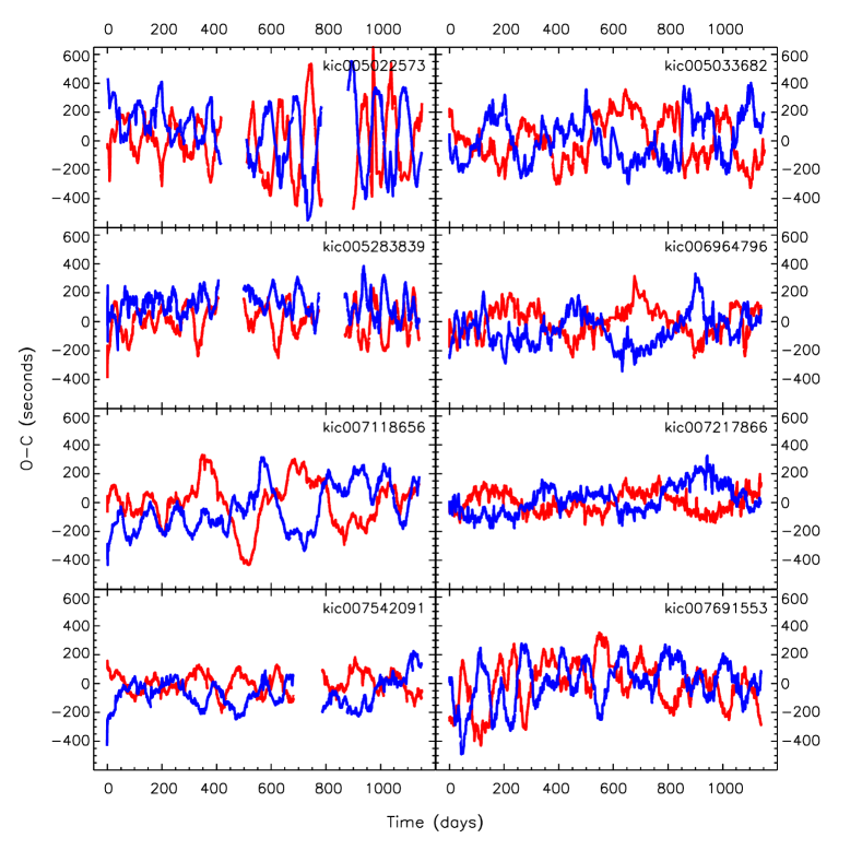
Figure 3.— A sample of $O-C$ curves for an illustrative set of eight contact binary systems with KIC numbers in the range of 5022573 to 7691553. The specifications are otherwise the same as for Fig. 2.

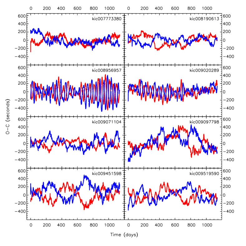
Figure 4.— A sample of $O-C$ curves for an illustrative set of eight contact binary systems with KIC numbers in the range of 7773380 to 9519590. The specifications are otherwise the same as for Fig. 2.

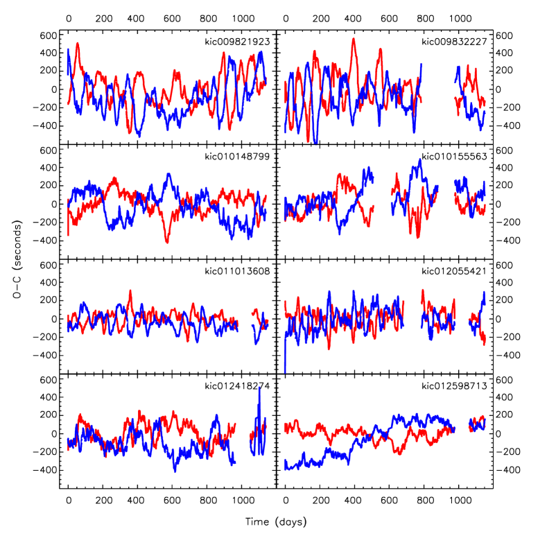
Figure 5.— A sample of $O-C$ curves for an illustrative set of eight contact binary systems with KIC numbers in the range of 9821923 to 12598713. The specifications are otherwise the same as for Fig. 2.

Once the times of the primary eclipses were found for each source, a linear function consisting of the eclipse cycle count times the orbital period taken from the Slawson et al. (2011) catalog was used in order to form an ‘observed minus calculated’ (or “$O-C$”) curve. If the binary orbit is circular and is not perturbed by a third body in the system, and if the shape of the eclipses remains constant, the $O-C$ curve should be a straight line.

In addition to the primary eclipses, $O-C$ curves were also calculated for the secondary eclipses of all the binary systems.

For each binary, the $O-C$ curve for the primary eclipse was fit with a linear function to determine the best average of the orbital period over the $\sim$3-year interval of the Kepler data set (Quarters 1-13). This corrected period was used to produce final $O-C$ curves for both the primary and secondary eclipses.

Since most of the interesting variations in the $O-C$ curves occur on time scales of weeks to months, the $O-C$ curves were smoothed to reduce the amplitudes of high-frequency variations without substantially degrading longer-term features. This procedure was accomplished by convolving each $O-C$ curve with a boxcar function with a five day duration, thereby typically averaging over some $10-15$ $O-C$ values, i.e., orbital cycles (see Fig. 1 for an illustrative sample). This operation, of course, will remove any physical $O-C$ variability on scales $\lesssim 5$ days, but there are some artifacts, e.g., beats between the orbital period and the Kepler long-cadence integration interval of 29.4 min, that make a search for short periodicities in the $O-C$ curves difficult.

3. Contact Binary $O-C$ Curves

In the process of examining the eclipse-timing-variation $O-C$ curves for all $\sim$2000 binaries, while searching for evidence for the presence of third bodies (Rappaport et al. 2013), we discovered that a very large fraction of the shorter period binaries had a set of common features in their $O-C$ curves. These features include (i) random-walk or quasi-periodic variations, and (ii) anticorrelated behavior between the $O-C$ curves of the primary and secondary eclipses. We found that some 390 of the short period binaries exhibited these features in their $O-C$ curves (see Table 1 for the numbers as a function of orbital period).

We used the numerical morphological classification scheme of Matijevič et al. (2012) to characterize the binaries that seem to exhibit both properties listed above. The results are displayed in Table 1. There are some 306, 49, 30, and 4 of these binaries in the orbital period ranges $0.2-0.5$, $0.5-1$, $1-2$, and $>2$ days, respectively. The mean, median, minimum, maximum, and standard deviation of the Matijevič et al. (2012) morphology parameter, $c$, are given for each orbital period category. It is clear that the systems of interest are mostly in the orbital period range $0.2-0.5$ days, where contact and overcontact binaries are found. The numbers fall off sharply with increasing orbital period.

The Matijevič et al. (2012) numerical morphological descriptor, between 0 and 1, is given for each binary. The sense of this classification scheme is that morphological values of $\lesssim$ 0.5 correspond to detached binaries, while values in the ranges $0.5-0.7$ and $0.7-0.8$ correspond to semidetached and overcontact binaries, respectively. Values higher than 0.8 are ellipsoidal light variables and “uncertain” classifications, and a number of these may not be eclipsing. As can be seen from Table 1, as well as by looking at the actual distribution of values, some 2/3 of the binaries of interest have $c\gtrsim 0.8$ and $\sim$1/3 have $0.7<c<0.8$. This implies that the vast majority of them are contact binaries, with a substantial fraction exhibiting largely ellipsoidal light variations (‘ELV’) rather than pronounced eclipses.

For contact systems, the transition between purely ELV behavior, partial eclipses, and full eclipses is a smooth one. Thus, we do not make a sharp distinction between eclipsing contact binaries of the W UMa class vs. contact binaries that exhibit pure ELVs. We therefore use the terms ‘eclipse times’ and ‘times of minima’, or ‘eclipses’ and ‘minima’, somewhat interchangeably.

Table 1 Binary Morphology Statistics

		$P_{\rm orb}$ (days)			This
Parameter	$0.2-0.5$	$0.5-1$	$1-2$	$~{}~{}~{}~{}~{}>2~{}~{}~{}~{}~{}$	Work
# Systems	306	49	30	4	32
$\langle c\rangle$	0.86	0.73	0.75	0.82	0.93
Median $c$	0.87	0.69	0.78	0.83	0.91
$\delta_{c}$	0.09	0.14	0.20	0.11	0.05
$c_{\rm min}$	0.65	0.53	0.47	0.68	0.81
$c_{\rm max}$	1.0	0.98	1.0	0.92	1.0

Note. — Binary morphology statistics for the short period Kepler binaries with anticorrelated $O-C$ curves for the primary and secondary minima (http://keplerebs.villanova.edu/; Matijevič et al. 2012). The morphology index, $c$ is defined such that detached systems have values $\lesssim 0.5$; semi-detached systems are in the range $0.5-0.7$; and overcontact binaries lie in the range $0.7-0.8$. Systems with morphology index above $\sim$0.8 are ellipsoidal variables and or uncertain categories.

3.1. Illustrative $O-C$ Curves for Contact Binaries

From the set of 390 systems whose $O-C$ curves exhibit (i) random-walk or quasi-periodic variations, and (ii) anticorrelated behavior between the primary and secondary eclipses, we selected 32 systems to display and discuss in some detail. These all fall into the period range of $0.2-0.5$ days, where the vast majority of these systems lie, but are otherwise indistinguishable from the other $\sim$275 systems that we identified in this period range. We focus on this set for the remainder of the paper. The morphology statistics of this group of 32 are summarized in Table 1.

The $O-C$ curves for these 32 illustrative systems are shown in Figs. 2 – 5, and some of the system parameters are listed in Table 2. There are several potentially important features to note about the selected sets of $O-C$ curves presented in this paper. The peak-to-peak amplitudes of the short-timescale random-walk like behavior are typically about 500 seconds, although a few systems exhibit somewhat higher amplitude variations. The latter includes KIC 5022573 (top left panel of Figure 3). The characteristic time scales of the quasiperiodicities vary greatly, but are often in the range of $\sim$50-200 days.

The selected $O-C$ curves also exhibit clear anticorrelated behavior on at least some time scales and for some time intervals, even when positive correlations between the primary and secondary curves are evident on relatively long time scales. For example, the $O-C$ curves for KIC 1873918 (see Figure 2) are anticorrelated over the 100-day time scales of their quasiperiodic variations, but show an overall positive correlation on timescales over $\sim$800 days.

For this sample of contact binaries, $O-C$ curves were also calculated for the times of the two maxima in each orbital cycle. The $O-C$ curves for the two maxima as well as the two eclipse minima of one of the contact binaries, KIC 9451598, are shown in Figure 6. The two $O-C$ curves for the eclipse maxima are clearly anticorrelated with respect to each other in the same way as are the $O-C$ curves for the minima. In addition, the plot suggests that the $O-C$ curves of the maxima are offset in phase from the curves of the minima by about 90^∘, i.e., that the rate of change in one curve is maximal at the amplitude extrema in the other curve. We attempt to explain both the 180^∘ and 90^∘ phase shifts with a simple starspot model in Sect. 4.

To demonstrate more quantitatively the anticorrelated behavior between the $O-C$ curves of the primary and secondary minima, we show a point by point correlation plot for one system: KIC 7691553 ($O-C$ curves shown in the bottom right panel in Fig. 3) in Fig. 7. To create this particular plot, the $O-C$ values were averaged in one-day time bins. The plot shows a clear negative correlation, and confirms what is seen in a visual inspection of the $O-C$ curves. The formal correlation coefficient is $-0.5$ for the particular example shown in Fig. 7. For systems that are dominated by anticorrelated $O-C$ curves, the correlation coefficients range down to $-0.77$, with a median value of $-0.42$.

In addition to computing and displaying correlation plots for the contact binaries in our sample, we also computed formal cross correlation functions (CCFs) for all the pairs of (one-day rebinned) eclipse $O-C$ curves. The plots mostly confirm the characteristic timescales observed in the $O-C$ curve variations, as well as the anticorrelated behavior at zero time lag.

Fourier transforms of the $O-C$ curves for our sample of contact binaries do not show, in general, any strong peaks, except for the known beat frequencies between the orbital period and the long-cadence sampling time (see Rappaport et al. 2013 for details). Plots of $\log A_{\nu}$ vs. $\log\nu$, where $A_{\nu}$ is the Fourier amplitude and $\nu$ is the frequency, generally show more or less linear relations with logarithmic slopes of approximately $-1.0$ to $-1.3$ that are similar to Fourier spectra associated with random-walk behavior.

4. Models

4.1. Period Changes

Most of the structure seen in the $O-C$ curves for the contact binaries cannot represent actual changes in the orbital periods (see Kalimeris et al. 2002 for a related discussion). The argument is simple. For circular orbits like those expected for contact binaries, period changes would produce similar, i.e., positively correlated, effects in both the primary and secondary $O-C$ curves. Therefore, the variations associated with anticorrelated behavior cannot be the result of orbital period changes.

In addition, mass transfer could not drive such rapid changes in the $O-C$ curves even if the primary and secondary eclipses were not anticorrelated. This may be understood quantitatively by representing a small portion of the $O-C$ curve as:

$$O-C\simeq\tau\sin(2\pi t/T)$$ (1)

where $\tau$ and $T$ are rough measures of the amplitude and cycle time of the undulations in the $O-C$ curve, and $t$ is the time. If the variations were caused by orbital period changes, the second derivative of the $O-C$ curve would be related to the first derivative of the orbital period as

$$\frac{\dot{P}_{\rm orb}}{P_{\rm orb}}=\frac{d^{2}\hbox{}}{dt^{2}}(O-C)=-\frac{4\pi^{2}}{T^{2}}\tau\sin(2\pi t/T).$$ (2)

It is straightforward to show that mass transfer in a binary results in $\dot{P}_{\rm orb}/P_{\rm orb}\approx\dot{M}/M$. Therefore, the implied mass transfer rate would be of order

$$\frac{\dot{M}}{M}\approx 4\pi^{2}\frac{\tau}{T^{2}}.$$ (3)

For characteristic $O-C$ amplitudes of $\sim\pm$200 seconds and cycle times of $\sim$50-200 days (see Figs. 2-5), we find implied mass transfer rates of $\dot{M}/M\simeq 0.001-0.01$ yr^-1. These rates are implausibly large even for a contact binary. More physically reasonable mass transfer rates have been inferred for contact binaries such as $\sim$$10^{-7}\,M_{\odot}$ yr^-1 in VW Boo, a typical overcontact binary (Liu et al. 2011), and in several W UMa systems (Borkovits et al. 2005).

4.2. Slightly Eccentric Orbits

The orbits of contact binaries must generally be circular or nearly circular. However, it is perhaps conceivable that perturbations from a third body, or even some stochastic mass-exchange, magnetic event, or other physical process could induce a very minor eccentricity from time to time. The apsidal motion that would then ensue would result in $O-C$ variations, to first order in eccentricity, with amplitudes of $\pm(P_{\rm orb}/2\pi)2e\cos\omega$ for the primary and secondary minima, respectively (Gimenez & Garcia-Pelayo 1983); $\omega$ is the longitude of periastron. Consequently, an $O-C$ amplitude of $\pm$300 sec in a binary with an orbital period of 0.3 days requires a minimum eccentricity of $\sim$0.04. Since this is implausibly high for a contact binary, slightly eccentric orbits are unlikely to be the cause of most of the anticorrelated behavior that is apparent in the observed amplitudes.

4.3. A Simple Starspot Model

4.3.1 Spot Visibility

Here we consider a simple geometric model wherein a single spot on one of the stars might produce the anticorrelated behavior seen in the timing of the primary and secondary minima. In this simplistic picture, the stars are taken to be spherical and to be rotating synchronously with the orbit. The $\hat{z}$ direction is defined to be parallel to the orbital angular momentum vector; the stars revolve in the $x-y$ plane. The observer is located in the $y-z$ plane and views the system with conventional orbital inclination angle $i$. The unit vector in the direction from the system toward the observer is then $\vec{V}=\cos i\,\hat{z}+\sin i\,\hat{y}$. For a spot located at colatitude $\alpha$, the angle from the stellar pole, and stellar longitude, $\ell$, the unit vector pointing from the center of the star through the spot is $\vec{S}=\sin\alpha\,\sin(\omega t+\ell)\,\hat{x}+\sin\alpha\cos(\omega t+\ell)\,\hat{y}+\cos\alpha\,\hat{z}$, where $\omega$ is the orbital angular velocity. A starspot located at $\ell=0^{\circ}$ and $\alpha=90^{\circ}$ is defined to lie along the line segment connecting the two stellar centers.

The spot is assumed to occupy a small portion of the surface of the star and is taken to radiate in a Lambertian manner. The projected area of the spot normal to the line of sight is proportional to the cosine of the angle between the normal to the spot area and the direction toward the observer, $\vec{V}\cdot\vec{S}$. If this dot product is negative, the spot is on the hemisphere of the star facing away from the observer and is not visible. When the dot product is positive, the spot is not occulted, and if limb darkening may be neglected, the apparent brightness of the star is changed by the presence of the spot according to the expression

$$\Delta F=\epsilon\left[\cos\alpha\cos i+\sin\alpha\sin i\cos(\omega t+\ell)\right]$$ (4)

where $\epsilon$ is a constant with dimensions of flux assumed to be much less than the overall flux from the binary. In order for the spot to remain continuously visible, $\Delta F$ must always be positive. Such a condition requires that $\cos\alpha\cos i>\sin\alpha\sin i$, or, equivalently, $\alpha+i<$ 90^∘.

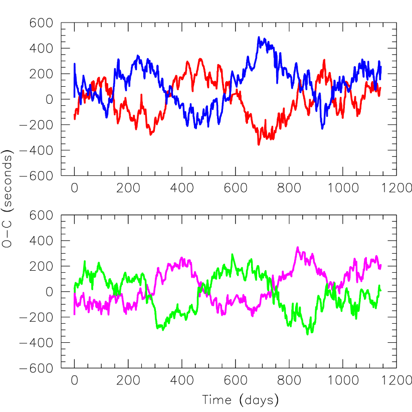
Figure 6.— The O-C curves for KIC 9451598 showing anticorrelated behavior between the minima (top panel) as well as the maxima (bottom panel). Note that the curves in the bottom panel are $\sim$90^∘ out of phase with respect to those in the top panel.

4.3.2 Analytic Estimate of the $O-C$ Amplitudes

When no spots are present, the light curve of a contact binary may be represented with sufficient accuracy by

$$\mathcal{B}=-B\cos 2\omega t$$ (5)

where time $t=0$ corresponds to the time of primary minimum (here indistinguishable from the secondary minimum) and where the constant term has been dropped. In this crude model, $B$ is the modulation amplitude due to both ellipsoidal light variations and eclipses.

When one spot is present, the observed flux as a function of time, again aside from constant terms, will then be:

$$\mathcal{F}=-B\cos 2\omega t+\epsilon\sin\alpha\sin i\cos(\omega t+\ell).$$ (6)

We can now examine analytically how the two minima and the two maxima are shifted in phase relative to the case of no spot. The analysis is straightforward since it is assumed that $\epsilon\ll B$ as mentioned above. After expanding the relevant trigonometric functions for small excursions about their nominal extrema, and neglecting high order terms, the four phase shifts, in radians, are found to be:

$$\Delta\phi_{\rm min,n} = -(-1)^{n}\,\frac{\epsilon\sin\alpha\sin i}{4B}~{}\sin\ell$$ (7)

$$\Delta\phi_{\rm max,n} = (-1)^{n}\,\frac{\epsilon\sin\alpha\sin i}{4B}~{}\cos\ell$$ (8)

where $n=1$ or 2 for the first or second, respectively, minimum or maximum.

It is immediately clear that (i) the shifts of the times of the two minima are anticorrelated; (ii) the shifts in the two times of maxima are anticorrelated; and (iii) the changes in the times of the two maxima are 90^∘ out of phase with respect to the times of the two minima. It is also clear from these expressions that the phase shifts depend on the spot longitude; a near uniform migration in longitude with time leads to a quasiperiodic $O-C$ curve.

In some timing analyses, the eclipse center is defined as the midpoint between the ingress and egress times, e.g., at their half intensity points. Perturbations to such eclipse centers can also be worked out analytically using the same formalism and approximations as discussed above. The corresponding shifts in the eclipse times are the same as given by eqn. (7), except that they are larger by a factor of $\sqrt{2}$.

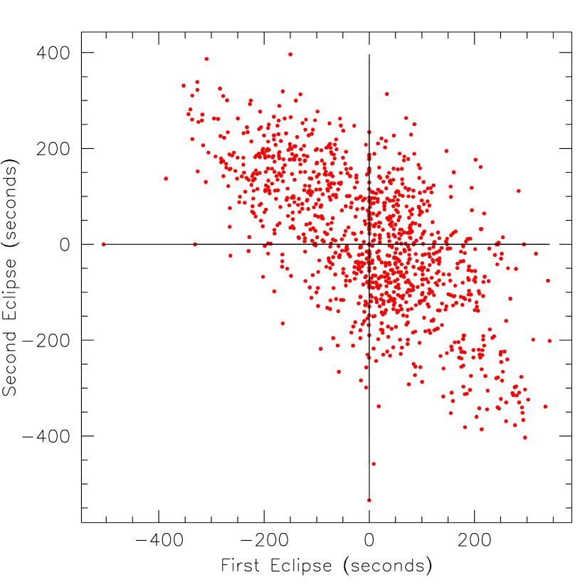
Figure 7.— A point-by-point correlation plot of the binned O-C curves for the primary and secondary eclipses of KIC 7691553. The negative slope of the plot clearly demonstrates the anticorrelation of the $O-C$ curves, with a correlation coefficient of $-0.5$.

The (half peak-to-peak) amplitude of the $O-C$ variations seen as the spot migrates around the star at constant $\alpha$ can be computed from eqn. (7) and is given in units of time by:

$$\tau=\frac{\epsilon\sin\alpha\sin i}{4B}\frac{P_{\rm orb}}{2\pi}$$ (9)

The coefficient quantifying the photometric strength of the spot may be estimated by

$$\epsilon\simeq\frac{4\Delta T}{T}\frac{\pi r_{\rm spot}^{2}}{\pi R_{\rm 1}^{2}}\frac{B_{0}}{2}$$ (10)

where $r_{\rm spot}$ is the radius of the spot, $R_{\rm 1}$ is the radius of the star with the spot, $\Delta T$ is the decrement (increment) in temperature of the cool (hot) spot, and $B_{0}$ is the mean brightness of the binary. Finally, if we define an eclipse depth in terms of the fractional decrease in intensity at the minimum, $\xi\equiv B/B_{0}$, the expression for the amplitude of the $O-C$ shifts becomes:

$$\tau=\frac{1}{4\pi\xi}\sin\alpha\sin i\frac{\Delta T}{T}\frac{r_{\rm spot}^{2}}{R_{\rm 1}^{2}}P_{\rm orb}.$$ (11)

For the illustrative parameter values of $\xi=0.04$, $\alpha=45^{\circ}$, $i=40^{\circ}$, $r_{\rm spot}/R_{\rm 1}=0.2$ (equivalent to a spot radius of 11.5^∘ of arc on the stellar surface), $\Delta T/T=0.15$, and $P_{\rm orb}=8.7$ hours, we find $\tau\sim$170 s, a value similar to those seen in the $O-C$ observations.

4.3.3 Eclipses and Spot Occultations

An eclipse in a binary system consisting of two spherical stars of radii $R_{1}$ and $R_{2}$ will only occur if the inclination satisfies

$$i\gtrsim\cos^{-1}\left[\frac{R_{1}+R_{2}}{a}\right]$$ (12)

If we use the Eggleton (1983) analytic approximation for the size of the Roche lobe for a range of mass ratios of $0.3\lesssim M_{2}/M_{1}\lesssim 3$, we find that $(R_{1}+R_{2})/a$ is very close to $\sim$0.76, corresponding to a minimum inclination angle of $\sim$$41^{\circ}$ (see Fig. 8).

Finally, this model only produces strictly anticorrelated primary and secondary $O-C$ curves if the spot is not occulted by the companion star. If the spot is not occulted when it is located at longitude $\ell=0$, then it will not be occulted when it is at any other longitude. A condition on the inclination angle to avoid occultation of the spot at $\ell=0$ is relatively straightforward to derive. If the radii of the star with the spot and the second star are $R_{1}$ and $R_{2}$ respectively, then the constraint can be written as one on the angle $\alpha$ as a function of inclination:

$$\alpha<\sin^{-1}\left[\frac{a}{R_{1}}\cos i-\frac{R_{2}}{R_{1}}\right]+i$$ (13)

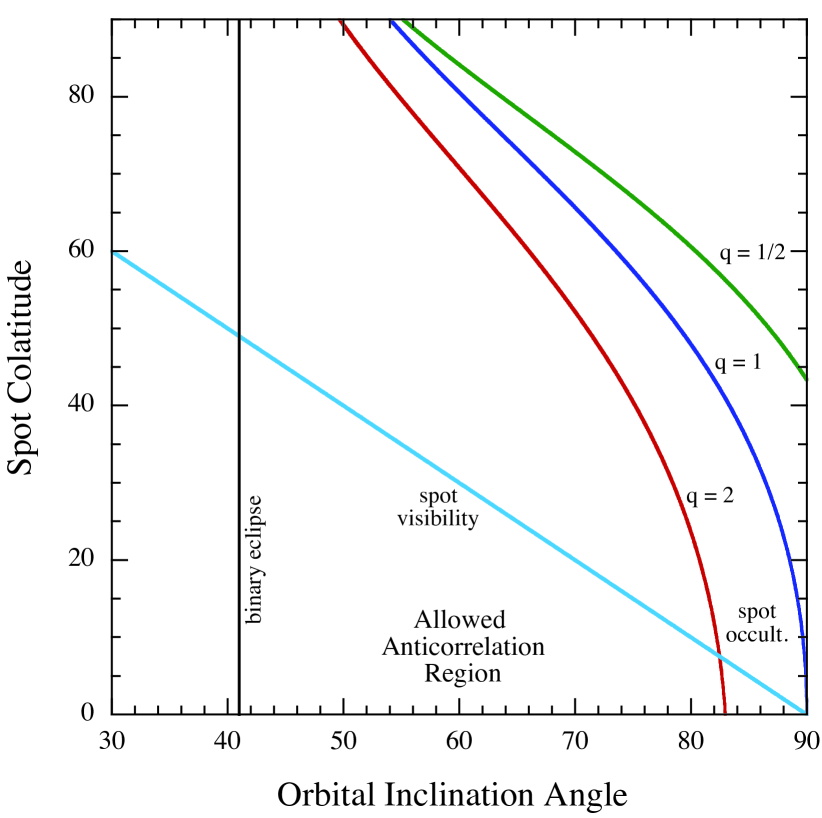
Figure 8.— Geometric requirements for the observer to be able to see a starspot around an entire orbit of an eclipsing binary. The allowed region lies below all the curves – which is essentially dictated by the diagonal spot visibility line. Eclipses will be seen for system parameters to the right of the vertical line, or even possibly above inclination angles as small as $34^{\circ}$. All angles are in degrees. The quantity $q\equiv M_{2}/M_{1}$. The relative stellar radii are computed from $q$ which dictates the relative sizes of the two Roche lobes.

The constraints on the inclination angle and the spot colatitude are summarized in Fig. 8. The spot colatitude is plotted on the y axis and the inclination angle on the x axis. Viable regions in this parameter space lie to the right of the vertical line at $41^{\circ}$, below the spot visibility line given by the requirement that $\alpha+i<90^{\circ}$, and below the curves given by eq. (13).

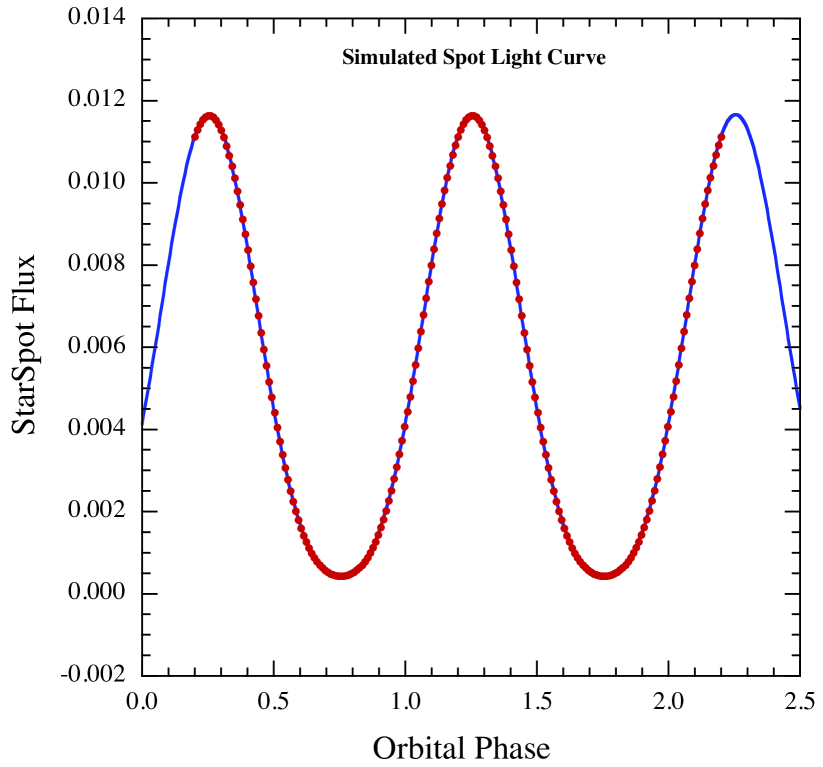
Figure 9.— Phoebe generated ‘light curve’ of a single hot spot. The red points are the relative flux coming from a hot spot as a function of the orbital phase. To generate these points we adopted the following spot parameters: colatitude $\alpha=45^{\circ}$, longitude $\ell=90^{\circ}$, radius = 10^∘, $T_{\rm spot}/T_{\rm star}=1.15$. The orbital inclination is $40^{\circ}$. The blue curve is a model fit to equation (5) in the text with $\ell$ set to 90^∘.

5. Light Curve Simulations with Phoebe

In order to verify the validity of some of the approximations used for our simple model, we utilized the Phoebe binary light curve emulator (Prša & Zwitter 2005) to model a contact binary system where either one cool or one hot spot may be present on one star. As a strictly illustrative model, we utilized the Phoebe fit to the folded light curve of KIC 3437800, a Kepler contact binary whose $O-C$ curves are also anticorrelated, though it is not included in the present sample of 32 systems. That fit yielded the parameters $P_{\rm orb}=8.7$ hours; $i=40^{\circ}$, $T_{\rm eff}=6185$ K, and $q=M_{2}/M_{1}=0.62$ that specify the baseline no-spot model. A hot or cold spot was then placed at one of a variety of locations on the surface of the primary star, and orbital light curves were simulated. The times of the four extrema (two minima and two maxima) were found using the same parabolic interpolation method used for the actual Kepler data. We emphasize that the system parameters adopted for KIC 3437800 are illustrative only.

For this particular example, the spot was positioned at $\alpha=45^{\circ}$, $\ell=90^{\circ}$, and was given a radius of 10^∘ on the surface of the primary and a temperature that was elevated by 15% over the local $T_{\rm eff}$ of the star. Fig. 9 shows the difference between the light curves of the models with and without the spot. The difference curve is not exactly a pure sine function. This can readily be understood in terms of limb-darkening, by modifying eq. (4) with a simple linear limb darkening law such that:

$$\Delta F_{\rm spot}\propto\cos\theta\left[1-u(1-\cos\theta)\right]$$ (14)

where $\cos\theta$ represents the dot product between the direction to the observer and the spot vector with respect to the center of its host star, and $u$ is the linear limb-darkening coefficient. Substituting in the expression for the dot product, we can write the above expression as:

$$\Delta F_{\rm spot} = A+b(1-u+2au)\cos(\omega t+\ell)+ub^{2}\cos^{2}(\omega t+\ell)$$

$$~{}~{}~{}~{}a \equiv \cos\alpha\cos i~{}~{}~{}~{}~{}~{}~{}{\rm and}~{}~{}~{}~{}~{}~{}~{}b\equiv\sin\alpha\sin i$$

where $A$ is a $DC$ offset. Basically, this is equivalent to equation (4) except for the addition of a $\cos^{2}$ term which accounts for the limb darkening. A best-fit curve of the form given by eq. (5) is superposed on the data obtained from the Phoebe simulations in Fig. 9. The fit is excellent.

Phoebe model light curves were then computed for cases with the spot centered at each of a set of longitudes covering the range $0^{\circ}\leq\ell\leq 360^{\circ}$, and still at a colatitude of $\alpha=45^{\circ}$. The $O-C$ results are shown in Fig. 10 for the two minima as well as the two maxima. It is immediately evident that the $O-C$ curves for the two minima are indeed anticorrelated, as are the curves for the two maxima; however, they are not pure sine curves. The nonsinusoidal behavior of the $O-C$ curves must differ from that in the simple model because limb darkening produces a lightcurve for the spot that is not exactly sinusoidal (see Fig. 9). When the analytic expressions for the phase shifts, as given in eqns. (7) and (8), are rederived while accounting for limb-darkening per eq. (5), highly analogous results are found except that the $\sin\ell$ term in eq. (7) is multiplied by a factor of $(1\pm\chi\cos\ell)$ while the $\cos\ell$ term in eq. (8) is multiplied by a factor $(1\pm\chi\sin\ell)$, where $\chi$ is a geometry-dependent number of order $1/3-1/2$. Therefore, even after including limb darkening, the $O-C$ curves for the primary and secondary minima (as well as for the two maxima) are still anticorrelated in the sense that their values always have opposite signs, however the magnitudes are not quite equal.

In Fig. 10 we show fits to the Phoebe-generated $O-C$ curves (filled circles) using the functions of $\ell$ given in eqns. (7) and (8), but with each multiplied by the extra factor discussed above. The free parameter $\chi$ was found to be consistent with 0.45 $\pm 0.04$ for all four curves. Since the fits are quite good, it appears that the simple model formalism captures the important aspects of the effects of starspots.

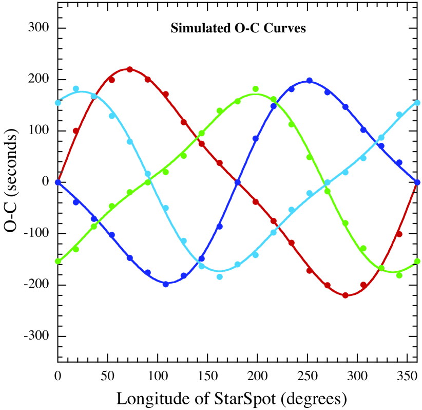
Figure 10.— $O-C$ curves generated by Phoebe for the binary system described in Fig. 9, and modeled after KIC 3437800. The red and blue points are for the primary and secondary eclipses, respectively, while the green and cyan points are for the out-of-eclipse maxima. The smooth curves are fits to a simple spot model, modified by limb darkening, as discussed in Sect. 5.

6. Discussion

The simple starspot model presented here to explain both the general appearance and amplitude of the $O-C$ curves for contact binaries, as well as the anticorrelations between the $O-C$ curves for the primary and secondary eclipses, seems to work remarkably well. At this point, it is natural to wonder to what degree similar effects, especially the anticorrelations between the $O-C$ curves for the primary and secondary eclipses, would be observable in longer period binaries.

First, and perhaps most importantly, in order for the present starspot model to be effective in producing visibly detectable anticorrelated $O-C$ curves, the stars in the binary would be required to rotate nearly synchronously with the orbit. With increasing orbital periods this becomes less and less likely. Second, for longer orbital periods, eclipses will only be seen in general for inclinations nearer to $90^{\circ}$. For larger inclination angles, starspots must be located nearer to the poles of the stars (see Fig. 8) to avoid being occulted during the eclipses. Not only will the unocculted region be smaller, but also spots may be less likely to occur near a stellar pole. Third, it is plausible that contact binaries are more likely to have large spots and that any spots on them tend to be larger than the spots on the stars in longer period binaries.

Finally, there will be a decrease in any $O-C$ amplitude due essentially to the smaller duty cycle of the eclipse in longer period binaries. For longer orbital periods, the eclipse duration is given in terms of orbital cycles by:

$$\frac{\Delta\theta_{\rm ecl}}{2\pi}=\frac{1}{\pi}\sin^{-1}\left[\frac{(R_{1}+R_{2})}{a}\right]\simeq\frac{(R_{1}+R_{2})}{\pi a}$$ (16)

where the approximation has been made that $R_{1}\sim R_{2}\ll a$. The eclipse profiles may be crudely approximated as in eq. (5) by taking $\mathcal{B}=-B\cos N\omega t$ for times $t$ near those for which $\omega t=0$ and $\omega t=\pi$. Here $N$ would be given by

$$N\simeq\frac{\pi}{\Delta\theta_{\rm ecl}}\simeq\frac{\pi a}{2(R_{1}+R_{2})}$$ (17)

In the discussion presented above, e.g., in eq. (5), we had taken $N=2$ to represent a contact binary. For stars of a fixed, typical, unevolved size, eq. (17) states that $N\propto a\propto P_{\rm orb}^{2/3}$. When the calculation that led to eqs. (7) through (11) is recast in terms of $N$ with all other parameters held fixed, the leading factor of $1/4$ becomes $1/N^{2}$. In turn, this implies that

$$\tau\propto\frac{P_{\rm orb}}{N^{2}}\propto P_{\rm orb}^{-1/3}$$ (18)

This result may be applied, in an extreme example, to a binary with a $\sim$30-day period, i.e., a period approximately two orders of magnitude longer than that of a typical contact binary. In a binary with this longer period the spot-induced $O-C$ variations would be reduced in amplitude by a factor of $\sim$5 over those of a contact binary comprising similar stars and having similar spots.

We note that in keeping with these conclusions, based on the spot model, close binaries are strongly favored to exhibit anticorrelated $O-C$ curves. Table 1 shows just how rapidly the anticorrelation phenomenon decreases with increasing orbital period.

Another question that arises in connection with the proposed starspot model is what happens to the basic equation for shifts in the timing, as in eq. (7), when there is more than one starspot present at the same time? The result is simply a sum of terms as given in eq. (7) but with a distribution of spot parameters, including different stellar longitudes – the latter being by far the most important. For the case where a single spot of a given area and temperature decrement is divided into $n$ smaller spots of the same total area, and assigned a random distribution of $\ell$ values, the net result will be a simple decrease in the amplitude of the resultant $O-C$ curve by roughly $\sqrt{n}$. Thus, even if there are, e.g., 10 smaller spots present on one star, the amplitude of the shifts in timing are likely to be reduced by only a factor of a few. If, by contrast, the number of spots increases to $n$, but their sizes and temperature decrements remain unchanged, then the amplitude of the $O-C$ curve increases by $\sqrt{n}$. In either case, these collections of spots still have to migrate in a semi-coherent way, if quasi-periodic behaviors in the $O-C$ curves are to be observed.

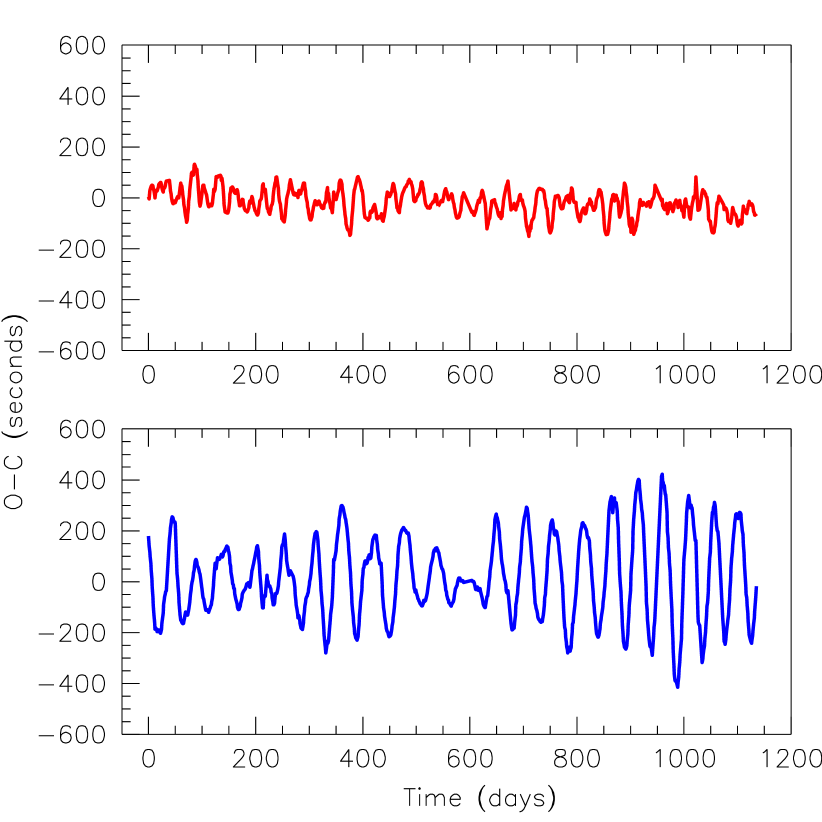
Figure 11.— The sum (top) and difference (bottom) of the $O-C$ curves (divided by 2) for the primary and secondary eclipses of KIC 8956957, respectively.

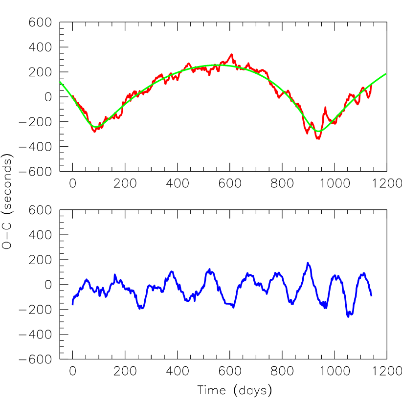
Figure 12.— The sum (top) and difference (bottom) of the $O-C$ curves (divided by 2) for the primary and secondary eclipses of KIC 1873918, respectively. The solid green curve on the top panel represents an orbital fit to the $O-C$ (see text for details).

The quasiperiodic $O-C$ variations with characteristic time scales $\sim$50-200 days should carry information about the surface differential rotation of the stellar components in our sample of contact binaries. Following Kalimeris et al. (2002) and Hall & Busby (1990), we use a differential rotation law of the form:

$$P_{\alpha}=\frac{P_{\rm orb}}{(1-k\cos^{2}\alpha)}$$ (19)

where, again, $\alpha$ is the colatitude of the spot, and $P_{\alpha}$ is the rotation period at colatitude $\alpha$. The migration period, $P_{\rm mig}$ is then:

$$P_{\rm mig}=\frac{P_{\rm orb}^{2}}{(P_{\alpha}-P_{\rm orb})}\simeq\frac{P_{\rm orb}}{k\cos^{2}\alpha}$$ (20)

where the right hand approximation is based on the assumption that $k\ll 1$. If the 50-200 day time scales are interpreted as migration periods, the values of $k$ must be in the range 0.003 – 0.013, in good agreement with, but covering a smaller range than, the values cited by Kalimeris et al. (2002) and Hall & Busby (1990).

Finally, we noted above that the $O-C$ curves for some systems show evidence of positive correlations between the primary and secondary curves on relatively long time scales. For contact binary systems with a high degree of anticorrelated behavior between the $O-C$ curves for the primary and secondary minima, there is a simple way to separate out most of the starspot-induced eclipse timing changes from most of the changes that represent other effects such as the perturbations due to third bodies. This involves forming the sum of the two $O-C$ curves, divided by 2, as well as the difference, divided by 2 (see also Conroy et al. 2013 who apply the same technique). The latter tends to emphasize the effects of starspot activity, while the former tends to remove them, and thereby possibly show more clearly any effects due to, e.g., a third body. These sum and difference curves are particularly illuminating for systems that show long timescale positively correlated $O-C$ curves, but with short timescale anticorrelated behavior. This is demonstrated in Fig. 11 for KIC 8956957. The top panel shows the average of the two $O-C$ curves, and indicates very little residual structure of interest. By contrast, the bottom panel, which shows the differences between the $O-C$ curves, clearly exhibits the quasiperiodic behavior that we attribute to a starspot (or spotted region).

Figure 12 shows sum and difference $O-C$ curves for KIC 1873918. In this case, the summed curve (top panel) shows long-term behavior that could be indicative of orbital motion induced by a third star. The superposed smoothed curve shows the results of fitting for both the Roemer delay and the physical delay (see, e.g., Rappaport et al. 2013, and references therein; Conroy et al. 2013), both due to the presence of a third star. The inferred physical delay for this system is very small, as expected from the short binary period and the much longer inferred orbital period of the third star. Aside from some residual small-amplitude modulations in the $O-C$ curve, presumably due to starspots, the fit is quite respectable. The fitted parameters are: $P_{\rm orb}\simeq 854$ days, eccentricity $\simeq 0.63$, longitude of periastron $\omega\simeq 251^{\circ}$, Roemer amplitude $\simeq 280$ s, and mass function $\simeq 0.032\,M_{\odot}$. This object was missed as a candidate triple-star system in the initial search by Rappaport et al. (2013) likely because of the effects of starspot activity.

Summed $O-C$ curves for all 32 of our illustrative sample of contact and ELV binaries were computed and examined for possible evidence of a third body. The results for some six of the systems show clear long term quadratic trends which correspond to constant rates of change in the orbital periods. Typical values of the quadratic terms are $\dot{P}_{\rm orb}\simeq 10^{-8}$ days/day, or $P_{\rm orb}/\dot{P}_{\rm orb}\simeq 0.1$ Myr. The presence of long term quadratic trends in the $O-C$ curves of overcontact binaries is not unusual. For example, Qian (2001a; 2001b) lists 42 systems that evidently exhibit such features. The mean value of $P_{\rm orb}/\dot{P}_{\rm orb}$ found by Qian (2001a) for 12 contact binaries is 2.7 Myr, and for an additional 10 classified as ‘hot contact binaries’ is 4.4 Myr. All but one of these has a positive sign, indicating a lengthening period. Several other systems are also listed elsewhere in the literature. The Qian (2001a) values for $\dot{P}_{\rm orb}$ thus represent a factor of $\sim$30 more slowly evolving periods than the handful that we are able to detect in the Kepler collection. The greater sensitivity of the Qian (2001a) results is due to the long historical baseline of the plates they utilized ($\sim$80 years vs. 4 years for the Kepler data base), in spite of the lower precision in timing the eclipses. We note, however, that larger detected values of $\dot{P}_{\rm orb}$ in contact binaries are not unprecedented, e.g., LP UMa has $P_{\rm orb}/\dot{P}_{\rm orb}\simeq 0.2$ Myr (Csizmadia, Bíró, & Borkovits 2003).

In any case, such quadratic trends observed for the Kepler binaries might indicate the presence of a third body in an orbit with a period much longer than $\sim$1200 days, i.e., the length of the Kepler data train utilized in this work. Or, such quadratic trends could possibly be explained by evolutionary effects, which manifest themselves via different forms of mass exchange between the stellar components. These could include mass transfer in the context of thermal relaxation oscillation theory (Lucy 1976; Webbink 1976; Webbink 2003), or via angular momentum loss driven by stellar winds and/or magnetic braking (see, e.g., van’t Veer 1979; Mochnacki 1981; van’t Veer & Maceroni 1989).

7. Summary and Conclusions

Kalimeris et al. (2002) and earlier works showed that photometric perturbations, and, in particular, starspots may affect measured $O-C$ curves, and that those perturbations are not properly interpreted in terms of orbital period changes. They noted that spot migration could produce (quasi)periodic effects in the O-C curves.

In this work, we have substantially extended these earlier results. We have used the Kepler data base for binary stars, and an analytic model to provide good insight into the timing effects of starspots seen in the $O-C$ curves. In particular, we identified a large sample of Kepler target short-period binaries (i.e., $P_{\rm orb}\lesssim 1/2$ day) that appear to manifest the effects of a single spot or a small number of spots on their $O-C$ curves; these quite often have the form of a random-walk or quasiperiodic behavior, with typical amplitudes of $\sim$$\pm$ 300 s. Most of these $O-C$ curves also exhibit a very pronounced anticorrelation between the primary and secondary minima.

We developed a simple idealized model that illustrates the major effects that starspots have on measured eclipse times. In particular we showed that a spot will, in general, affect the times of primary minimum and secondary minimum differently, with the predominant effect being an anticorrelated behavior between the two, provided that the spot is visible around much of the binary orbit. We also showed that a spot can equally well affect the times of the two maxima in each orbital cycle, and that the effects on the two maxima should be different, typically including anticorrelated behavior between them and a 90^∘ phase shift with respect to the eclipse minima.

All of the same types of timing behavior are expected for close binaries that do not eclipse at all, i.e., so-called “ELV” binaries, and in fact, a significant fraction of the $\sim$390 binary systems exhibiting these properties may be in this category. There is probably even a selection effect whereby the anticorrelation properties of the $O-C$ curves are enhanced in binaries that either do not eclipse or which have only partial eclipses. The reason is that if an eclipse also occults a starspot over a substantial range of longitudes, $\ell$, on the surface, then the anticorrelation effect will be diminished. We can even turn this argument around and suggest that the detection of anticorrelated $O-C$ curves tends to indicate that the system being observed is a binary, as opposed to a false positive, such as a pulsator. This gives us some confidence that the four systems listed in Table 2 marked as false positives by Matijevič et al.(2012) are, in fact, actual binaries.

We have found that a few of the selected contact binaries showed positively correlated variations in the $O-C$ curves for their primary and secondary minima on long time scales as well as the anticorrelated variations that are most evident on shorter time scales. We then demonstrated that sum and difference $O-C$ curves between the primary and secondary eclipses are useful in distinguishing between the two types of variations. We used this latter technique (i.e., of summing the two $O-C$ curves of the primary and secondary eclipses) to better isolate the effects of a possible third body in the system. In the process we found a likely Roemer delay curve for one of the systems, as well as convincing evidence for a long-term quadratic trend in six other systems.

Finally, we found that the $O-C$ difference curves often appear to be dominated by 50 to 200 day quasiperiodicities that we interpret in terms of the migration of spots, due to differential rotation, relative to the frame rotating with the orbital motion.

Table 2 Kepler Contact Binaries with Anticorrelated $O-C$ Curves

Source	Binary Period	Morphology1	Magnitude	$T_{\rm eff}$	Correlation	Minimum 1	Minimum 2
KIC #	(days)	$(0-1)$	($K_{p}$)	(K)	Coefficient2	Depth3	Depth3
18739184	0.332433	0.86	13.72	5715	0.42(5)	0.104	0.099
20178034	0.305742	0.97	14.61	5056	-0.50	0.046	0.036
2159783	0.373886	0.87	14.96	5643	-0.16	0.217	0.194
2715007	0.297107	0.87	14.73	5598	0.10	0.025	0.018
3837677	0.461984	0.94	15.55	5466	-0.46	0.104	0.096
3853259	0.276648	1.00	13.92	4467	-0.42	0.076	0.073
49373504	0.393664	-1.00	14.27	5862	-0.60	0.072	0.068
5008287	0.291878	0.93	15.31	5881	-0.34	0.050	0.048
5022573	0.441724	0.98	11.47	5648	-0.13	0.056	0.056
5033682	0.379916	0.95	13.26	5611	-0.63	0.056	0.034
5283839	0.315231	0.92	15.16	5906	0.09	0.160	0.146
6964796	0.399966	0.97	12.61	5657	-0.52	0.050	0.044
7118656	0.321355	0.94	15.03	5271	-0.24	0.052	0.040
7217866	0.407157	0.90	13.86	5600	-0.15	0.106	0.093
7542091	0.390499	0.81	12.34	5673	-0.31	0.154	0.143
7691553	0.348309	0.93	14.62	5786	-0.48	0.092	0.088
7773380	0.307577	0.94	14.47	5357	-0.40	0.084	0.066
8190613	0.332584	0.90	15.13	5384	-0.28	0.117	0.113
8956957	0.324382	0.96	13.98	6307	-0.72	0.056	0.054
9020289	0.384027	0.94	14.74	5997	-0.60	0.061	0.059
9071104	0.385213	0.81	13.65	5959	-0.52	0.158	0.130
9097798	0.334068	1.00	14.58	5592	-0.41	0.027	0.026
9451598	0.362349	0.93	13.63	6060	-0.77	0.041	0.030
9519590	0.330895	0.88	13.92	5961	-0.24	0.039	0.036
9821923	0.349532	0.95	14.21	5730	-0.53	0.087	0.083
9832227	0.457950	0.94	12.26	5854	-0.19	0.094	0.086
10148799	0.346605	0.91	15.41	5340	-0.66	0.068	0.037
10155563	0.360268	0.94	11.99	5982	- 0.03	0.017	0.013
110136084	0.318287	-1.00	12.57	6223	-0.33	0.048	0.044
12055421	0.385607	0.96	12.52	6118	-0.47	0.041	0.038
12418274	0.352723	0.93	14.35	5215	0.22	0.050	0.038
12598713	0.257179	0.94	12.76	5189	-0.14	0.013	0.008

Note. — All parameters, unless otherwise specified, are from http://keplerebs.villanova.edu/ (Matijevič et al. 2013). (1) The binary light curve morphology index is defined such that detached systems have values $\lesssim 0.5$; semi-detached systems are in the range $0.5-0.7$; and overcontact binaries lie in the range $0.7-0.8$. Systems with morphology index above $\sim$0.8 are ellipsoidal variables and or uncertain categories. Systems with -1 are unclassified. (2) A description of how the correlation coefficients were computed is given in Sect. 3.1. (3) Depths of the primary and secondary minima in our folded light curves. (4) These systems are labeled as “binary false positives” by the Kepler team. We believe that the anticorrelated light curves provide evidence that they are, in fact, binaries. (5) The significant positive correlation for this system arises from the likely Roemer delay in the $O-C$ curve due to the possible presence of a third body.

References

- Awadalla, et al. (2004) Awadalla, N.S., Chochol, D., Hanna, M., & Pribulla, T. 2004, CoSka, 34, 20
- Barnes et al. (2004) Barnes, J. R., Lister, T. A., Hilditch, R. W., & Collier Cameron, A. 2004, MNRAS, 348, 1321
- Batalha et al. (2010) Batalha, N.M., Borucki, W.J., Koch, D.G, et al. 2010, ApJ, 713, L109
- Batalha et al. (2013) Batalha, N.M., Rowe, J.F., Bryson, S.T., et al. 2013, ApJS, 204, 24
- Borkovits et al. (2005) Borkovits, T., Elkhateeb, M. M., Csizmadia, Sz., Nuspl, J., Bíró, I. B., Hegedüs, T., & Csorvási, R. 2005, A&A, 441, 1087
- Borucki et al. (2010) Borucki, W. J., et al. 2010, Science, 327, 977
- Caldwell et al. (2010) Caldwell, D.A. 2010, ApJ, 713, L92
- Conroy et al. (2013) Conroy, K. E., Prša, A., Stassun, K. G., Orosz, J. A., Fabrycky, D. C., & Welsh, W. F. 2013, submitted to ApJ [arXiv: 1306.0512]
- Csizmadia et al. (2003) Csizmadia, Sz., Bíró, I.B., & Borkovits, T. 2003, A&A, 403, 637
- Csizmadia et al. (2004) Csizmadia, Sz., Patkós, L., Moór, A., & Könyves, V. 2004, A&A, 417, 745
- Csizmadia et al. (2006) Csizmadia, Sz., Kővári, Zs., Klagyivik, P. 2006, Ap&SS 304, 355
- Csizmadia & Klagyivik (2004) Csizmadia, Sz. & Klagyivik, P. 2004, A&A, 426, 1001
- Eggleton (1983) Eggleton, P. P. 1983, ApJ, 268, 368
- Eggleton (2006) Eggleton, P. P. 2006, Evolutionary Processes in Binary and Multiple Stars. ISBN 0521855578. Cambridge, UK: Cambridge University Press.
- Eggleton (2012) Eggleton, P. P. 2012, JASS, 29, 145
- Fabrycky & Tremaine (2007) Fabrycky, D. & Tremaine, S. 2007, ApJ, 669, 1298
- Gazeas & Stepień (2008) Gazeas K. & Stepień K. 2008, MNRAS, 390, 1577
- Geske et al. (2006) Geske, M. T., Gettel, S. J., & McKay, T. A. 2006, AJ, 131, 633
- Gimenez & Garcia-Pelayo (1983) Gimenez, A., & Garcia-Pelayo, J.M. 1983, ApJS, 92, 203
- Hall & Busby (1990) Hall, D. S., & Busby, M. R. 1990, in Active Close Binaries, ed. C. Ibanoǧlu (Dordrecht: Kluwer), 377
- Hendry & Mochnacki (2000) Hendry, P.D. & Mochnacki, S.W. 2000, ApJ, 531, 467
- Jenkins et al. (2010a) Jenkins et al. 2010a, Society of Photo-Optical Instrumentation Engineers (SPIE) Conference Series, Vol. 7740
- Jenkins et al. (2010) Jenkins et al. 2010b, ApJ, 713, L87
- Kähler (2002) Kähler, H. 2002, A&A, 395, 899
- Kähler (2004) Kähler, H. 2004, A&A, 414, 317
- Kalimeris et al. (2002) Kalimeris, A., Rovithis-Livaniou, H., & Rovithis, P. 2002, A&A, 387, 969
- Kiseleva et al. (1998) Kiseleva, L. G., Eggleton, P. P., & Mikkola, S. 1998, MNRAS, 300, 292
- Koch et al. (2010) Koch, D.G., et al. 2010, ApJ, 713, L79
- Kozai (1962) Kozai, Y. 1962, AJ, 67, 591
- Lanza & Rodonó (1999) Lanza, A. & Rodonó, M. 1999, A&A, 349, 887
- Li et al. (2004) Li, L., Han, Z., & Zhang, F. 2004, MNRAS, 351, 137
- Li et al. (2008) Li, L., Zhang, F., Han, Z., Jiang, D., & Jiang, T. 2008, MNRAS, 387, 97
- Liu et al. (2011) Liu, L., Qian S.-B., Zhu, L.-Y., He, J.-J., & Li, L.-J. 2011, ApJ, 141, 147
- Lucy (1968) Lucy, L. B. 1968, ApJ 151, 1123
- Lucy (1976) Lucy, L. B., 1976, ApJ, 205, 208
- Maceroni et al. (1994) Maceroni, C., Vilhu, O., van’t Veer, F., & van Hamme, W. 1994, A&A, 288, 529
- Maceroni & van’t Veer (1996) Maceroni, C. & van’t Veer, F. 1996, A&A, 311, 523
- Matijevic et al. (2012) Matijevič, G., Prša, A., Orosz, J.A., Welsh, W.F., Bloemen, S., Barclay, T. 2012, AJ, 143, 123
- Mochnacki (1981) Mochnacki, S.W. 1981, ApJ 245, 650
- Morris (1999) Morris, S. 1999, ApJ, 520, 797
- Paczyński et al. (2006) Paczyński, B., Szczygieł, D. M., Pilecki, B.; Pojmański, G. 2006, MNRAS, 368, 1311
- Pop & Vamos (2012) Pop, A., & Vamos, C. 2012, New Astr, 17, 667
- Pribulla & Rucinski (2008) Pribulla, T. & Rucinski, S. M. 2008, MNRAS, 386, 377
- Prsa & Zwitter (2005) Prša, A., & Zwitter, T. 2005, ApJ, 628, 426
- Qian (2001a) Qian, S. 2001a, MNRAS, 328, 635
- Qian (2001b) Qian, S. 2001b, MNRAS, 328, 914
- Qian (2003) Qian, S. 2003, MNRAS, 342, 1260
- Rappaport et al. (2013) Rappaport, S., Deck, K., Levine, A., Borkovits, T., Carter, J., El Mellah, I., Sanchis-Ojeda, R., & Kalomeni, B. 2013, ApJ, 768, 33
- Robertson & Eggleton (1977) Robertson, J. A., & Eggleton, P. P. 1977, MNRAS, 179, 359
- Rucinski (1998) Rucinski, S. M. 1998, AJ, 116, 2998
- Senavci et al. (2011) Senavci, T., Hussain, G. A. J., O’Neal, D., & Barnes, J. R. 2011, A&A 529, 11
- Slawson et al. (2011) Slawson, R., et al. 2011, AJ, 142, 160
- Smith et al. (2012) Smith, J. C., Stumpe, M. C., Van Cleve, J. E., et al. 2012, PASP, 124, 1000
- Stepień & Gazeas (2012) Stepień, K. & Gazeas, K. 2012, AcA, 62, 153
- Stumpe et al. (2012) Stumpe, M. C., Smith, J. C., Van Cleve, J. E., et al. 2012, PASP, 124, 985
- van’t Veer (1979) van’t Veer, F. 1979, A&A 80, 287
- van’t Veer, F. & Maceroni (1989) van’t Veer, F. & Maceroni, C. 1989, A&A 220, 128
- Vilhu et al. (1988) Vilhu, O., Caillault, J-P., & Heise, J. 1988, ApJ, 330, 922
- Webbink (1976) Webbink, R. 1976, ApJ, 209, 829
- Webbink (2003) Webbink, R.F. 2003, in 3D Stellar Evolution, ASP Conf. Ser., Vol. 293, eds. S. Turcotte, S. C. Keller, & R. M. Cavallo, p. 76
- Wilson (1994) Wilson, R. E., 1994, PASP 106, 921
- Yakut & Eggleton (2005) Yakut, K. & Eggleton, P. P. 2005, ApJ, 629, 1055