A Topological Extension of General Relativity to Explore the Nature of Quantum Space-Time, Dark Energy and Inflation

Abstract

General Relativity is extended into the quantum domain. A thought experiment is explored to derive a specific topological build-up for Planckian space-time. The presented arguments are inspired by Feynman’s path integral for superposition and Wheeler’s quantum foam of Planck mass mini black holes/wormholes. Paths are fundamental and prime 3-manifolds like $T^{3}$, $S^{1}\times S^{2}$ and $S^{3}$ are used to construct quantum space-time. A physical principle is formulated that causes observed paths to multiply: It takes one to know one. So topological fluctuations on the Planck scale take the form of multiple copies of any homeomorphically distinct path through quantum space-time.

The discrete time equation of motion for this topological quantum gravity is derived by counting distinct paths globally. The equation of motion is solved to derive some properties of dark energy and inflation. The dark energy density depends linearly on the number of macroscopic black holes in the universe and is time dependent in a manner consistent with current astrophysical observations, having an effective equation of state $w\approx-1.1$ for redshifts smaller than unity. Inflation driven by mini black holes proceeds over ${\rm n}\approx 55$ e-foldings, without strong inhomogeneity, a scalar-to-tensor ratio $r=ln(7)/{\rm n}\approx 0.036$ and a spectral index $n_{s}=1-r\approx 0.964$. A discrete time effect visible in the cosmic microwave background is suggested.

PACS numbers: 04.20.Gz; 98.80.Hw; 04.60.Pp; 95.36.+x; 04.70.Dy

1 Introduction

General Relativity (GR) is one of the most beautiful and succesful physical theories.^1,2 It links the action of gravity to the geometry of space-time. GR’s extension to the quantum domain has been explored over many years by many authors, e.g., quantum foam ideas for geometric dynamics, loop quantum gravity, loop algebras for quantum connectivity in four dimensions, spin foams that suggest a lower effective dimensionality of space-time and string theory that requires a much higher dimensionality.^{3,4,5,6,7,8,9,10,11,12,13}

Early work in Refs. 3-5 on the Wheeler-deWitt equation already considered quantum geometric dynamics through a sum over all possible 3-geometries, including topologically non-trivial ones. In this, a proper measure and factor ordering were identified as problems. Another line of research that goes beyond pure geometry is loop quantum gravity. In it, well chosen operators allow one to quantize space-time geometry and derive important insights into the quantum properties of BHs.^6,7 Also, the ideas of Mach, a great motivation for Einstein, are still powerful today in the form of approaches that highlight the fundamental importance of background independence.¹⁴ Indeed, although local formulations of physical laws have proven to be very succesful, a truly self-consistent universe appears only to be constructable if one explicitly incorporates a global notion of space-time using topology.^12,13

In this context, Wheeler’s quantum foam of Planck mass mini black holes (BHs) or wormholes remains an intuitively appealing picture of quantum space-time. The lack of conformal invariance in the Einstein equation leads to the inevitable presence of large metric fluctuations. Also, the Schwarschild BH is a perfectly fine solution of the Einstein equation. This while the evaporation of BHs, as well as the thermodynamic laws that their horizons obey, makes them the perfect entities to bridge classical and quantum space-time.^15,16 Of course, quantum space-time may host more than just mini BHs and likely calls for a completely new structure altogether.

Nevertheless, the absence of topology in GR, while it predicts BHs, suggests that the mere continuity of space-time may hold important clues to quantizing it. Also, if the unstable nature of the quantum foam could be remedied, i.e., if its (effective) energy density is lowered in a controlled manner, then this may help to resolve the discrepancy between the large expected vacuum energy and the perceived low value of present-day dark energy.^{17,18,19,20,21}

Furthermore, topology deals with connectivity while geometry pertains to shape. The connectivity of space-time, i.e., the existence of homeomorphically distinct paths between arbitrary points $A$ and $B$, lies at the heart of quantum physics. It is the path integral formulation of Feynman that shows how the superposition principle is an expression of path multiplicity.²² The fact that many of the paths in Feynman’s path integral are continuous but not differentiable favors an a priori topological approach. Finally, if one views paths as fundamental, then Nature must have some way to construct them and assert that they are truly distinct. This is a highly non-trivial task in the presence of the quantum uncertainty in Planck scale geometry discussed above.^3,4

This work therefore finds its inspiration in Wheeler’s quantum foam and Feynman’s path integral formulation for quantum superposition, and uses topology as the natural language of quantum space-time. The efforts in Refs. 12 and 13, which use algebraic topology to define quantum geometry, are taken as a basis. These are elaborated upon to highlight the crucial role of a multiply (so non-simply) connected space-time for quantum gravity, dark energy and inflation.

The section below presents a thought experiment that provides a physical basis for the mostly mathematical considerations of Ref. 12. Subsequently, the equation of motion for the “topological dynamics” of quantum gravity is derived, and solved under certain approximations to explore the nature of dark energy and its relation to inflation. In all, this paper is self-contained.

2 Topological Dynamics

2.1 Thought Experiment: The Multiplication of Paths

Consider the following thought experiment for an observer who wishes to assess the structure of his space-time through some measurement process. Excluding the philosophically interesting case of a completely isolated observer, it seems reasonable to assume that the observer can detect phenomena and come to some quantitative view of his universe through a measuring apparatus. What properties of space-time should the observer measure and how can he quantify these?

Going back to the introduction of this paper, it is good to recall the central tenet of quantum physics: the superposition principle. At the root of all quantum phenomena lies the notion of space-time paths. It is with paths that the fabric of space-time can be woven and the superposition principle of quantum physics be expressed, at the same time.

Most straightforwardly the observer can start by choosing a few (material) objects and measuring the paths these objects take to map out properties of space through time. While doing so for smaller and smaller objects and decreasing scales, he will encounter the distinct paths that quantum particles travel along. For example, when he performs the well known double slit experiment and identifies interference effects because electrons follow a multitude of routes.

At this stage, he can start to quantify the properties of his space-time by identifying different classes of paths. E.g., one class of paths contains all those paths that go through slit 1 and another class those that go through slit 2. Of course, the two classes of paths are a priori a consequence of matter (the double slit), but the observer decides to extend his experiments all the way to the Planck scale to explore the spirit of superposition.

On the Planck scale, geometric fluctuations in space-time are large and inhibit him to perform accurate measurements. This does not surprise him because the lack of conformal invariance of the Einstein equation already implies this quantum behavior. However, these fluctuations do not preserve the shape of space-time, while the observer wants to measure what paths comprise space-time despite any such quantum uncertainty in geometry.

He then recalls the double slit experiment, with the two distinct classes of paths, and realizes he can still measure paths that cannot be obtained from each other by simply changing the shape of space. I.e., paths are detectable if they cannot be transformed into each other through a homeomorphism of space-time. Consequently, the properties of such paths are assessable by the observer.

But, when taking a good look at his, by now formidable, measuring apparatus, it is also obvious to him that he is as much observer as actor in these experiments. The quantum uncertainty in geometry that plagues him, is as much caused by his apparatus as it is a consequence of the lack of conformal invariance in GR. While performing experiments in this manner, he develops the following insight. It is through the observational comparison of paths that one comes to an assessment of their identity, and thus the structure of quantum space-time. As such, no path can exist, or remain to exits, on its own when scrutinized and the observer thinks: “It takes one to know one. So topological fluctuations on the Planck scale take the form of multiple copies of any homeomorphically distinct path through quantum space-time.”

So due to Planckian quantum effects, the very act of identification requires paths to multiply, in 4-space. Although puzzled, the observer also realizes that the minimal form that any identification of an entity takes, is to at least count it. Apparently, his counting of paths is prone to quantum fluctuations with pertinent consequences for Planckian space-time.

The observer then summarizes his observational acts as follows. The minimal form of space-time path identification is to count them. In order to count paths, he must confirm their existence by recognizing their intrinsic properties. This requires at least a proper example to observationally compare to and implies a sense of multiplicity, if he is to make any quantitative sense of space-time and its quantum geometric uncertainty on the Planck scale.

Being somewhat mathematically inclined, the observer recognizes the importance of distinction when speaking of paths and their multiplicity. Path distinction is the expression of homeomorphic inequivalence. I.e., using the symbol $\sim$ for equivalence, paths $X$ and $Y$ that obey $X\sim Y$ belong to the same class $[X]$ because a continuous map transforms one into the other. Hence, to assert that there are paths $[X]$ the observer concludes that he must have at least one other class $[X^{\prime}]$ to compare to. For example, consider a landscape with a bridge. One can walk along many paths $[X]$ across the bridge and these paths are all topologically distinct from those paths $[Z]$ that choose to cross the water. The comparison class $[X^{\prime}]$ then simply represents all those paths crossing another bridge.

Pondering this some further, the observer realizes that he is only one and that Nature herself needs to take on the task of counting distinct space-time paths. In doing so unremittingly, the very act of counting distinct paths must result in pertinent and persistent changes to the structure of scrutinized quantum space-time.

The observer concludes that the nature of these multiplicative changes preserves the intrinsic topological properties of the original paths. That is, quantum fluctuations in geometry are merely incidental on the Planck scale. It is the connectivity of the bridge mentioned above that matters, not its shape. Furthermore, when counting that bridge, the interaction between observer and observee requires Nature to build at least one other bridge. If Nature would not, then no proper confirmation of a path’s identity is possible at all. Because first cause lies in the act of identification (counting), path multiplication is an expression of observation.

In everyday life such a notion appears untenable, but on the Planck scale it has long been argued^3,4 that any formal measurement on the order of a Planck time, using a Planck mass worth of energy, must lead to a space-time with topologically exotic objects like wormholes, loops, etc. I.e., Planckian space-time is multiply connected, supporting a plethora of homeomorphically distinct paths that are caused by the act of observation.

This space-time path multiplication phenomenon, first discussed for local paths in Ref. 12 and referred to as induction for BHs in Ref. 13, is elevated here to a fundamental physical property of quantum space-time: the multiplicity principle (MP). It is formulated as follows.

Paths that are distinct under the continuous deformation of space-time constitute a fundamental observable property of space-time. To confirm the identity of such paths on the Planck scale, they must at least be countable. Under the observational act of counting, no distinct path can (remain to) exist individually. If it would, then its intrinsic properties would be unknown and its fundamental nature undefined. Instead, it takes one to know one. So, when scrutinized by any observer, these distinct paths must multiply and thus build quantum space-time. Therefore, topological fluctuations on the Planck scale take the form of multiple copies of any homeomorphically distinct path through quantum space-time.

The above considerations are in line with usual quantum phenomenology, in which no formal distinction can be made between observer and observee, and interactions between them affect both in a pertinent manner. The MP allows Nature to distinguish paths, despite any quantum uncertainty in geometry, using topology. The MP also forces Nature to treat paths as dynamical entities on the Planck scale, requiring multiplication. The information on the (number of) different equivalence classes of paths is distributed through homeomorphisms. This information therefore constitutes a global quantity. I.e., topology cares only for integer numbers, and a Machian perspective on the universe results.

2.2 Quantum Space-Time Structure

The MP can be reworded as that one single path modulo homeomorphisms has the same physical significance as no path. Or equivalently, that the minimal¹² building block of space-time is the loop $S^{1}$. That is, a loop is the combination of two paths from A to B such that one cannot be deformed into the other by a homeomorphism.

2.2.1 The Prime Manifolds $T^{3}$, $S^{1}\times S^{2}$ and $S^{3}$

When dealing with space-time, so with 4 dimensions, the natural building blocks are so-called prime 3-manifolds and their number evolution in time. Any topologically non-trivial space-time manifold^23,24,25 can be constructed by adding together 3-primes, embedded in 4 dimensions, through a connected sum. These 3-primes (e.g., handles, three-tori, three-spheres) lend their name from the property that they themselves cannot be written as the connected sum of smaller 3-dimensional units. Furthermore, interactions among prime manifolds can never change their intrinsic properties, like the number of closed loops they contain.

The MP then dictates that the path dynamics of any 4-dimensional quantum space-time must be carried by 3-primes that contain pairs of paths through their $S^{1}$ loop make-up. Once a basis set of 3-primes is chosen, the MP also imposes that quantum space-time is constructed by them. In Refs. 12 and 13 a 3-prime basis set has been proposed that consists of the three-torus $T^{3}$, the handle $S^{1}\times S^{2}$ and the three-sphere $S^{3}$. In this work, somewhat different arguments are presented but the same basis set of 3-primes is found.

1) A multiply connected space-time should be locally flat and locally isotropic in the absence of gravity. Using the $S^{1}$ loop, there is only one 3-prime that is locally isotropic and non-simply connected. This is the three-torus²³, $T^{3}=S^{1}\times S^{1}\times S^{1}$. The three loops that $T^{3}$ contains require it to be embedded in four dimensions. Indeed, the three loops are topological identifications, through the fourth dimension, of the front-back, top-bottom and left-right surfaces that form the boundaries of the solid cube $I^{3}$.

When confined to the Planck scale, the three-torus also introduces, in a local sense, the homeomorphically distinct paths that are needed for the superposition principle as expressed by Feynman’s path integral.²² Note that the Euler characteristic of $T^{3}$ is zero, so it is the boundary of a Lorentz 4-manifold.

2) The Einstein equation enjoys the Schwarzschild solution for a macroscopic BH. The latter constitutes the low energy limit of Wheeler’s quantum foam. I.e., Planckian BHs are transient under Hawking evaporation while macroscopic BHs are among the most stable entities in the universe on entropic grounds. One should note then that the loop containing handle $S^{1}\times S^{2}$ is just like the Schwarzschild BH solution when one considers Hawking evaporation in 4-space, as follows.

Even a macroscopic BH evaporates very slowly. So, in a topological sense, the Schwarzschild BH allows a connection between different times for accreted versus radiated mass-energy. It is therefore topologically equivalent to a handle $S^{1}\times S^{2}$, which connects different spatial regions, when one treats a macroscopic BH as a time-dependent embedding in 4-space. One could consider the handle or BH as a bridge between entirely different universes, with orthogonal sets of dimensions. However, a single multiply connected 4-space is considered to be the universe here, albeit with many superposed quantum histories (see further in section 2.2.3).

In this work, there is no limitation imposed by the null energy condition. Planckian wormholes evaporate on the order of a Planck time. Macroscopic BHs only possess a wormhole topology across cosmically separated time slices (probably in a completely incoherent fashion). Obviously, a countable quantity like the number of BH event horizons is invariant under homeomorphisms of four-dimensional space-time. Note that the Euler characteristic of $S^{1}\times S^{2}$ is zero, so that it is also the boundary of a Lorentz 4-manifold.

3) When one counts pairs of distinct paths, there should be the possibility of finding zero. With the loop being the central object of a multiply connected space-time, the zero represents the absence of loops and thus a simply connected space-time. The latter is equivalent to the three-sphere $S^{3}$ and homeomorpisms thereof. Diffeomorphisms are a subset of all homeomorphisms. The coordinate invariance of shape should therefore appear as one goes to large $S^{3}$ scales (see further in section 4.2).

One can then conclude that a plausible basis set consists of the non-chiral prime 3-manifolds $T^{3}$, $S^{1}\times S^{2}$ and $S^{3}$, where 1) the three-torus is confined to the Planck scale and carries local isotropy and superposition for a multiply connected space-time; 2) the non-irreducible handle appears as the large scale solution of the Einstein equation, i.e., the Schwarzschild BH; 3) the topologically trivial three-sphere represents the zero loop space-time, i.e., the unit element for path multiplication.

2.2.2 Construction through the Connected Sum

With the basis set in place, it is necessary to apply the MP. Starting with $T^{3}$, a space-time with a single three-torus cannot exist by itself. Rather, the act of counting multiplies it. Even though embedded in 4-space, $T^{3}$ is a 3-prime and its paths in 3-space proceed through the six faces that it possesses. Hence, the multiplication of three-tori that the MP requires can only connect the additional three-tori through 3-dimensional junctions (homeomorphic to the solid cube). In other words, one has a lattice.

Such a lattice of three-tori can be constructed by performing a connected sum. I.e., by using three-ball surgery to connect each face of a three-torus to a face of another three-torus through a junction. So a lattice $L$ of three-tori can be written as

$$L(T^{3})=\oplus^{i}T^{3}_{i},$$ (1)

where $\oplus$ denotes a connected sum. The Einstein summation convention is adopted and $i$ can be arbitrarily large unless noted otherwise. It is important to realize that the origin of $\oplus^{i}T^{3}_{i}$ in Eq. (1) lies purely in the topological dynamical consequences that application of the MP has. That is, only connected pairs of three-tori have comparative meaning.

The construction of the lattice can be performed along each of the 6 directions defined by the 6 faces. Subsequently, one can always apply a homeomorphism $H$ that relocates the junctions between three-tori. Hence, for $i>>1$ and all homeomorphisms $H_{k}\{L(T^{3})\}$, the equivalence classes $[H_{k}\{L(T^{3})\}]_{p}$ contain all distinct paths $p$ on $L(T^{3})$. Einstein gravity that bends $L(T^{3})$ on large scales is then naturally allowed by a subset of smooth homeomorphisms.

Through $L(T^{3})$, the motion of matter, like a particle world line, derives from a superposition of wave amplitudes along many different paths. One thus obtains, from the MP and expressed by the topology of space-time, the superposition principle as formulated by the Feynman path integral. Many of the paths that enter the Feynman path integral are continuous, but not necessarily differentiable. This is in the spirit of the homeomorphic invariance that underlies the approach in this work. The constructed distinct paths are now expressed, independent of quantum uncertainty in geometry, by the global multiply connected character of quantum space-time.

Furthermore, handles can be attached to the lattice of three-tori through the connected sum as well. This structure is denoted by $L(T^{3})^{+}$, i.e.,

$$L(T^{3})^{+}=L(T^{3})\oplus\ [\oplus^{j}(S^{1}\times S^{2})_{j}],$$ (2)

for arbitrary $j$. Because of the homeomorphic freedom of the connected sum, handles can connect to three-tori as well as other handles. The simply connected three-sphere $S^{3}$ embodies the freedom of homeomorphisms and one has that

$$T^{3}\oplus S^{3}\sim T^{3},$$ (3)

and

$$S^{1}\times S^{2}\oplus S^{3}\sim S^{1}\times S^{2}.$$ (4)

Even with the heuristic application of the MP, it is therefore possible to construct a continuous quantum space-time from 3-primes that possesses, dynamically active, global paths based on connected $S^{1}$ loops. Information on the number of connected three-tori and handles is distributed through homeomorphisms, as already mentioned above. That is, the number of three-tori and the number of BHs are global, Machian, quantities. Knowledge of these dimensionless integer numbers is accessible to all Planckian observers. This while acquisition of such information proceeds without violation of causality because homeomorphisms allow any two quantum space-time points to be infinitesimally close. The latter point deserves further elaboration.

2.2.3 The Wave Function of the Universe

One may wonder how an observer can physically know about the formation of a BH far-away from him. The essence lies in being an observer on the Planck scale, so that the equivalence classes $[H_{k}\{L(T^{3})^{+}\}]_{p}$ are fully available. Then note the following.

In classical 4-space, one can see past events and their future consequences combined into one. In quantum space-time this is augmented with the notion of superposition. Taking a global perspective on quantum events then leads to a wave function of the universe $\psi$, and one that enjoys correlations spanning across space and time. On macroscopic scales, every day experience tells us that classical processes tend to dominate over quantum correlated ones. However, on the Planck scale the converse is true.

Hence, the formation of a BH involves the irreducible collapse of $\psi$ to a state with one extra BH. The universe as a whole, and all Planckian observers in it, then occupies a new state in the present. This while before, the universe was in a superposition of states that involved both the succesful and unsuccesful creation of the BH.

As long as all the chains of events, all the space-time paths $p$, that lead to a particular present can be distinguished homeomorphically on $L(T^{3})^{+}$, then the collapse of $\psi$ is a global event. Specifically, it is one that is global for all Planckian observers in terms of countable topological quantities like BHs, three-tori and the paths through them. The nature of the information involved in the formation of a BH (just a single integer number) is thus crucial here. This while the distribution of this information is an integer change within $\psi$.

There is a clear analogy here with the superposition of two electrons, in a joint up/down spin state, that are moved macroscopically far apart. Observation of one electron in an up state leads to wave function collapse and the instantaneous implementation of the down state for the other electron, and vice versa. The reason is that no information needs to be exchanged causally upon wave function collapse. This has already been taken care of while creating the macroscopic superposition in the first place.

Similarly, the formation of a BH is a history, one of many, that ends with a quantum mechanically leaky event horizon. In 3-space, at some moment in time, such an event causes local geometric disturbances that travel causally from its source. In 4-space, the formation of a handle constitutes a topological change that globally distinguishes one time-like slice through 4-space from another, by a single bit of information.

Indeed, experiments similar to the double slit experiment mentioned above appear not to produce an interference pattern if a single bit of information labels a path²⁶, and Schrödinger’s entanglement is destroyed. Analogously, BH formation leads to the selection and distinction of (and thus a choice for) a particular path through 4-space. These points will be returned to in the following sections, but the qualitative argument is as stated here.

2.3 Intermezzo: The $S^{1}$ Loop in Explorations of Quantum Gravity

In a phenomenological sense, the importance of loops is of course well recognized in other fields as well, e.g., loop quantum gravity and the theory of closed strings.^6,7,8,9,10 To place the explorations of this work in context, one can note the following.

2.3.1 Loop Quantum Gravity

The main motivation for loop quantum gravity, in terms of physical perspective, lies in the determination of space-time curvature. The latter is most elegantly defined through a closed path integration, which brings out curvature as the differences between parallel transported vectors.²⁵ When the loop is elevated to a fundamental geometric object, one can succesfully quantize geometry and derive important properties on the spectrum of the BH event horizon. Also, loop quantum cosmology appears to be free of a big bang singularity. In this, invariance under diffeomorphsms is adhered to as motivated by GR.

Loop quantum gravity and topological dynamics share their appreciation for, and implementation of, background independence. The main difference between them lies in the topological nature of the MP. I.e., in the global characterization of quantum space-time using homeomorphisms and the multiplication of (pairs of) paths as the operative aspect of quantization.

2.3.2 String Theory

The mathematics underlying string theory are beautiful. The 2-spin excitation that the string possesses as well as the AdS correspondence are very promising. Nevertheless, any string (closed or open) inhabits a higher-dimensional background space-time that needs to be provided for a priori. Even though the mathematical necessity for such an embedding space is clear, and driven by anomaly cancellation, the origin and evolution of these extra dimensions lies beyond the physical principles of string theory.

In string theory, the $n$-fold torus $T_{n}$ is the connected sum of two-tori $T^{2}=S^{1}\times S^{1}$. So, for $i=1$ to $i=n$,

$$T_{n}=\oplus^{i}T^{2}_{i}.$$ (5)

The n-fold torus is the result of closed string interactions because individual $S^{1}$ loops map out cylinders that build up $T_{n}$ when glued together. Such a structure nicely removes the single point interactions that plague particle field theory. Like $L(T^{3})$, the manifold $T_{n}$ is multiply connected. That being said, the difference in dimensionality between $T_{n}$ and $L(T^{3})$ is fundamental. While the MP helps one to build a quantum space-time, $T_{n}$ describes string interactions and not space-time itself.

However, one can identify an interesting connection between string theory and topological dynamics. If $\partial$ is the boundary operator²⁵ with the usual property

$$\partial^{2}=0,$$ (6)

then

$$\partial T^{3}=0\ \ \&\ \ \partial T^{2}=0.$$ (7)

Hence, ignoring boundary terms and noting that $\partial D^{2}=S^{1}$ for the solid disk $D^{2}$, one has that

$$L(T^{3})=\oplus^{i}[T^{2}\times\partial D^{2}]_{i}.$$ (8)

Now imagine that the two topologically identified spatial dimensions of $T^{2}$ are much larger, by a factor of $n$ compared to the Planck length, than the third $S^{1}$ boundary of $D^{2}$. The latter then represents much higher energies and constitutes a rapidly varying phase that stores its effects in the membrane $D^{2}$. Because of the large metric fluctuations that occur on the Planck scale, it is natural to identify this $\partial D^{2}$ with the metric component of Wheeler’s quantum foam.

That is, for the analysis in this section the Planck size surface $D^{2}$ is assumed not to be transformed into an event horizon $S^{2}$, which would require handles to be attached to $L(T^{3})$. Under these conditions, for $n^{2}>>1$ but small compared to the total number of three-tori in $L(T^{3})$, one finds locally for $i=1$ to $i=n^{2}$ that

$$L(T^{3})\approx[\oplus^{i}T^{2}_{i}]/n^{2}\times\partial D^{2}=\frac{T_{n}}{n^{2}}\times\partial D^{2}.$$ (9)

The sub-lattice $\oplus^{i}T^{2}_{i}$ has a weight $1/n^{2}$ because there are two independent directions in $T_{n}$ (it is a surface) that are each sampled with a duty cycle of $1/n$ relative to $\partial D^{2}$. The occurrence of a weight as part of the connected sum in Eq. 9 may seem odd. However, this weight simply counts the relative multiplicity with which components are connected. In Eq. (9), one has a ratio of $1/n^{2}$ $T_{n}$ to 1 $\partial D^{2}$. So only 1 of $n^{2}$ loops in $T_{n}$ is connected to $\partial D^{2}$. The above allows one to properly work, despite homeomorphic invariance, with fractions of otherwise integer topological quantities.

The above brings out $T_{n}$ as a lower-dimensional large scale topological perturbation for $n^{2}>>1$. I.e., $T_{n}$ is a slowly varying amplitude of $L(T^{3})$ and one that only weakly affects the rapid phase changes carried by the surface $D^{2}$. This because a Planckian observer on $\partial D^{2}$ can only count a (small) $1/n^{2}$ fraction of the total number of closed string interactions on $T_{n}$ during a Planck time.

In all, the heuristic value of the $S^{1}$ loop is beyond doubt. It is the physical principle guiding its use as a mathematical building block that sets at least a few of the various approaches to quantum gravity apart.

3 An Equation of Motion for the Evolution of Quantum Space-time

So far, the discussion has been mostly heuristic. To make quantitative progress, an equation of motion should be derived for the evolution of quantum space-time and it must be solved to make falsifiable predictions. In Ref. 12 a mathematical derivation is presented of a quantum space-time equation of motion, employing loop algebraic topology. A more physical derivation is presented here.

3.1 Physical Derivation: Counting Globally Distinct Paths

The key in the derivation of the equation of motion is 1) to incorporate the MP through proper counting of paths that are embodied by the basis set of 3-primes; and 2) to embrace the discrete nature of a topologically based quantum space-time all the way to time itself.

3.1.1 Right Hand Side

First, one recalls that basic connectivity, i.e., the need to travel from A to B, requires homeomorphically distinct paths. The minimal duo being the loop $S^{1}$. Second, one reasons that the existence of the loop-containing prime 3-manifolds $T^{3}$ and $S^{1}\times S^{2}$ follows directly from Feynman (superposition) and Wheeler (quantum foam), respectively. Third, one counts all loops in 3-primes self-consistently using the MP, every Planck time.

An observer, or rather Nature, who wishes to identify a three-torus can do so while approaching a $T^{3}$ along any of 6 spatial directions (top, bottom; front, back; left, right). In order to assess the properties of the three-torus from some side, within a Planck time, the MP requires an additional three-torus. The same holds for all neighboring directions, also within a Planck time. Combined, this implies that the complete identification of a three-torus under the MP requires 6 additional copies, and thus a multiplication factor of 7.

For the handle, the same logic applies. Albeit that a handle constitutes a bridge and counting can proceed only on either side of the bridge. This yields 2 sides, spatially separated for a handle and temporally separated for a slowly evaporating BH, from which to assess the nature of the handle/BH. The MP then imposes two additional copies, every Planck time, and thus a multiplication by a factor of 3.

One can formulate the numerical considerations above in terms of the action of the differential counting operators $\delta_{i}$, with $i=0$ for the three-torus, $i=1$ for the handle and $i=2$ for the three-sphere, as

$$\delta_{i}P_{i}=\mu_{i}P_{i},$$ (10)

for the 3-prime manifolds $P_{i}$, with

$$\mu_{0}=6\ \ \&\ \ \mu_{1}=2\ \ \&\ \ \mu_{2}=0.$$ (11)

Therefore, a single BH/three-torus becomes a triplet/heptaplet of BHs/three-tori under the MP. This confirms the need for a lattice of three-tori under the MP. However, BHs carry mass and are subject to Hawking evaporation. So, the MP imposes additional pairs of BHs with a success that depends on the longevity of existing BHs.

3.1.2 Left Hand Side

For the left hand side of the equation of motion one first realizes that the MP deals with global properties, basically just countable numbers. Furthermore, as mentioned before, homeomorphisms acting on $L(T^{3})^{+}$ allow for causally close proximity between any two space-time points. This is not to say that space-time is static, but rather that only a 1st order in time differential is needed for the left hand side, as with the Schrödinger equation. Furthermore, the nature of the time variable (which will be addressed in more detail below) has to be taken as discrete.

Afterall, even though the mathematical basis of quantum space-time derives from continuity, physically measurable quantities that are globally accessible to a Planckian observer are integer numbers only. Hence, when speaking of space, one does so in units of the Planck volume $l_{P}^{3}$ for the Planck length $l_{P}\approx 1.6\times 10^{-33}$ cm. While for time the proper unit is the Planck time $t_{P}\approx 5.4\times 10^{-44}$ s.

When counting as the MP requires, the massless three-torus has its 4-space dimensions specified by $l_{P}$ and $t_{P}$. However, the handle carries mass. Therefore, the natural unit of mass for a handle/BH that results from multiplication in the equation of motion is the Planck mass $m_{P}\approx 2.2\times 10^{-5}$ g. The counted numbers of three-tori and handles are denoted by the multiplicities $n_{i}$ and one has that

$$\Delta n_{i}P_{i}=n_{i}(m+1)P_{i}-n_{i}(m)P_{i},$$ (12)

for discrete times $(m+1)t_{P}$ and $mt_{P}$, in physical units, and integer steps $m=0,1,2,...\$.

3.1.3 Final Form: Discrete Time Evolution of 3-Prime Multiplicities

The correct connection between the left hand side and right hand side again involves the MP. Evolution is simply $\Delta n_{i}$. However for the counting of 3-primes on the right hand side only a single three-torus and handle have been considered, with $\mu_{0}=6$ and $\mu_{1}=2$. Of course, the act of counting is performed unremittingly. Therefore, the total multiplication that one incurs under the MP is $\delta_{i}n_{i}P_{i}$. This yields

$$\Delta n_{i}P_{i}=\delta_{i}n_{i}P_{i}=\mu_{i}n_{i}P_{i}.$$ (13)

Because the index $i$ already labels the 3-primes $P_{i}$ on which the operators act, one can also suppress the appearance of $P_{i}$ and write

$$\Delta n_{i}=\delta_{i}n_{i}=\mu_{i}n_{i}.$$ (14)

Note that there is no topologically dynamical role for the basis 3-prime $S^{3}$, as would be expected since

$$\Delta n_{2}S^{3}=\delta_{2}n_{2}S^{3}=0.$$ (15)

However, for the handles/BHs there are matter degrees of freedom that play a role as well. Afterall, the number of BHs changes as BHs form by gravitational collapse, evaporate by quantum processes or merge when brought into close proximity.

These processes are denoted by $F$ (formation), $E$ (evaporation) and $M$ (merging), respectively. Because such effects change the multiplicity $n_{1}$, they are also subject to the discrete time variable $m$ and written as $\Delta F$, $\Delta E$ and $\Delta M$. Going from one Planck time to the next, and adding the matter degrees of freedom terms to the right hand side, one thus finds the quantum space-time equation of motion as

$$\Delta n_{i}=\delta_{i}n_{i}+\delta_{1i}(\Delta F-\Delta E-\Delta M),$$ (16)

with $\delta_{1i}$ the usual Kronecker delta. Equivalently, explicitly including discrete time dependence as well as the masses that BHs have, one has

$$n_{i}(m+1)=(\mu_{i}+1)n_{i}(m)+\delta_{1i}(\Delta F(m+)-\Delta E(m+)-\Delta M(m+)),$$ (17)

where $(m+)$ denotes the change $\Delta$ during the continuous time interval $(m,m+1)$. Proper accounting of $n_{1}(m)$ under formation, evaporation and merging is assumed. I.e., $\Delta F=1$ means the formation of one BH (hence the plus sign). Also, $\Delta E=1$ means that one BH has evaporated during one time step (hence the minus sign), while $\Delta M=1$ means that two BHs have merged into one (minus sign). Naked singularities may in principle form and these could yield $\Delta E=0$ after an evaporation event. Gravitational lensing observations may be used to confirm the possible existence of naked singularities.¹⁶

It should be noted, and this is discussed further below, that $n_{1}(m)$ pertains to BHs of all masses, from the Planck mass to Solar masses and more. This is particularly relevant for the $\Delta E(m+)$ term. So one can best write $n_{1}(m)[\{M_{k}\}]$ (and also include charge and angular momentum if they play a role) for the masses $M_{k}$ that BHs $k=1...n_{1}(m)$ have. For ease of writing, this will typically be suppressed and $n_{1}$ is used.

3.1.4 GR and the Equation of Motion

Eq. (17) appears quite simple, but this is slightly misleading because the matter degrees of freedom term after the Kronecker delta affects the number of handles $n_{1}$ in a manner that potentially involves the full impact of GR.

Indeed, the evolution of the handle multiplicity $n_{1}$ is in part determined by the formation, evaporation and merging of black holes. These processes depend on the cosmic evolution of the energy-momentum tensor and space-time curvature tensor in the Einstein equation. Afterall, the occurrence of structure in the universe is intimately tied to the formation of massive stars, their BH stellar remnants, the subsequent dynamical interactions between those BHs, and their accretion histories.

Therefore, the longevity and transience of all BHs comes into play through the right hand side of Eq. (17). As such, “extension” appears to be the correct terminology for the topological approach pursued in this work. Eq. (17) serves GR, as follows.

GR remains completely valid down to the Planck scale as long as care is taken to include the effects of induced BHs and BH evaporation into the Einstein equation. These effects are determined in sections 5.1 (dark energy and accelaration today), 6.2 (dark energy and inflation in the early universe) 6.3 (amplitude of mass-energy fluctuations) and 6.5 (scaling properties of mass-energy fluctuations). When included, then the terms $\Delta F$, $\Delta E$ and $\Delta M$ can be computed as one would otherwise do when following the evolution of energy-momentum and curvature.

It will turn out that these corrections leave the form of GR unaffected. That is, GR can be extended all the way to the Planck scale in its usual formulation of $G_{\mu\nu}+\Lambda g_{\mu\nu}=8\pi GT_{\mu\nu}$, for the Einstein tensor $G_{\mu\nu}$, the cosmological constant $\Lambda$, the metric tensor $g_{\mu\nu}$ and the energy-momentum tensor $T_{\mu\nu}$.

This is because the evolution of $n_{1}$ due to Eq. (17) finds a natural place in $\Lambda$ (sections 5.1 and 6.2), leaving $G_{\mu\nu}$ unaffected. While the statistical properties (sections 6.3 and 6.5) of $T_{\mu\nu}$ in its standard form are completely specified by topological dynamics. Therefore, the beautiful properties of GR are completely preserved under the topological extension further explored below.

3.1.5 The Initial State and Superposition

The natural initial condition for Eq. (17) is a single $T^{3}$ as the start of a multiply connected 4-space at $m=0$. On this $T^{3}$ quantum fields can live with matter degrees of freedom and therefore the possibility to form the first BH(s) through GR. This way, quantum superposition in the form of distinct paths on a three-torus in 4-space is what forms the initial cause for our universe.

Multiplied three-tori and induced BHs, in every time slice $m$, carry no spatial information. When created, the connected sum assures that all 3-primes within a time slice are linked through junctions homeomorphic to $S^{3}$. Thus assuring that there are no island universes, but only a single path connected 4-space.

3.2 A Topological Extension of Mach’s Principle

Before solving Eq. (17) under certain circumstances, there is an immediate result that can be read off in the context of Mach’s principle. The quantum foam stability problem that plaques GR on the Planck scale, as explored by Wheeler, may find a natural resolution in the quantum space-time equation of motion above. If one considers the limit where

$$\Delta n_{1}=\Delta M=\Delta F\approx 0,$$ (18)

so a static or very slowly evolving population of handles with little classical BH formation and merging due to matter degrees of freedom, then

$$2n_{1}\approx\Delta E.$$ (19)

The quantum foam instability problem is solved if $n_{1}$ in Eq. (19) pertains to long-lived BHs. I.e., if there is an ensemble of BHs that lives for discrete times $mt_{P}$ at least comparable to the current age of the universe, then this population of $n_{1}$ long-lived BHs must cause the evaporation of twice that many induced BHs every Planck time. Afterall, for $n_{1}(m+1)\approx n_{1}(m)$ the evaporation term $\Delta E$ must act on not more than the Planck time for consistency.

The natural mass for these associated mini BHs is the Planck mass, if they are to evaporate in a Planck time. This while the evaporation time of a BH scales as its mass to the third power. So a BH of more than $2\times 10^{15}$ g would live as long as 10 billion years. Hence, an ensemble of macroscopic BHs provides a naturally stable quantum foam of Planckian mini BHs because of the MP. This leads to the quantum foam that Wheeler envisioned, but one that is constrained by the longevity of macroscopic BHs.

Einstein’s interpretation of Mach’s principle states that the global distribution of matter somehow determines the (changes in) local geometry, and vice versa. Wheeler’s local quantum foam of mini BHs, with its multiply connected topology, is an expression of GR. Therefore, following Einstein’s ideas for geometry with the MP for topology, matter that is globally observed to be in the form of macroscopic BHs somehow determines the (changes in) Planck scale topology, and vice versa. One may thus go one step further and use the MP to derive the topological extension of Mach’s principle (EMP). It is formulated as follows.

The global topology and geometry of the universe determine the changes in Planck scale topology and the local motions of matter, and vice versa.

This EMP is in essence the answer to the following question: How does Nature know what quantum fluctuations in geometry to provide for, in every Planckian volume? The answer suggested here, is that the collective action of all long-lived BHs provides this. Although strange, the EMP is in the spirit of Mach’s and Einstein’s ideas, with some help of the MP.

The number of macroscopic BHs in the entire universe, so in all of 3-space for some time slice through 4-space, is therefore the global quantity that determines the local occurrence of mini BHs in Wheeler’s quantum foam. Because of homeomorphic invariance, there is no specific volume to which induced mini BHs couple. However, despite being global principles, the MP and the EMP together do constrain this volume.

To speak of a Machian universe in the extended topological sense, there should be a stable global topology. That is, the inducing population of macroscopic BHs should have a longevity $m^{\prime}t_{P}$ that exceeds the age $mt_{P}$ of the universe at that time (the existence of a global time coordinate is addressed in section 4 below). Furthermore, the MP dictates that Eq. (19) already holds for a single long-lived BH and that any local observer of the quantum foam can determine the (growing) number of such macroscopic BHs.

This renders the first occurrence of a long-lived BH a locally and globally observable quantity on $L(T^{3})^{+}(m)$ in 4-space. I.e., paths that enter such a BH connect to a topologically distinguishable future $m^{\prime}>m$. So, if $L_{f}$ is the size of the universe when the first BH forms that exists for longer than the contemporary age of the universe, then $L_{f}$ is frozen in and the quantum foam stabilizes. That is, even though topological in origin, $L_{f}$ in Planck lengths is above all a geometric number that quantifies the first embedding volume $L_{f}^{3}$ of our universe in 4-space. The scale $L_{f}$ will be re-addressed in the context of dark energy in section 5 below.

3.3 Some Further Solutions: Exponential Self-Multiplication and Decay

Besides the Machian solution above, Eq. (17) can be also be solved straightforwardly under other approximations. For example, if $\Delta F=\Delta E=\Delta M\approx 0$ then

$$n_{i}(m+1)-n_{i}(m)\approx\mu_{i}n_{i}(m),$$ (20)

with the approximate exponential solutions

$$n_{0}(m)\approx 7^{m}$$ (21)

and

$$n_{1}(m\geq x)\approx 3^{m-x},$$ (22)

for initial conditions of the universe at $m=0$ that involve a single $T^{3}$ and with a first $S^{1}\times S^{2}$ formed by matter degrees of freedom after a short time $xt_{P}$ ($x<10$). Hence, quantum space-time can experience a self-multiplication phase that very quickly builds up a lattice of three-tori with an (unstable) foam of mini BHs attached to it. Such a state for the quantum foam will re-addressed in the context of inflation in section 6 below.

For the three-tori, which are always confined to the Planck scale contrary to the BHs, there are no further solutions unless one allows for reversals of the arrow of time. For the handles, there is also the situation where $\Delta F<<\Delta E$ and $\Delta M<<\Delta E$ over extended ($m>>1$) periods. In this limit one has that

$$n_{1}(m+1)-n_{1}(m)\approx\mu_{1}n_{1}(m)-\Delta E,$$ (23)

and for $-\Delta E+2n_{1}(m)\equiv-Dn_{1}(m)<0$, with $D<<1$, that

$$n_{1}(m+1)-n_{1}(m)\approx-Dn_{1}(m),$$ (24)

if the radiation background in the universe is low enough to allow all induced mini BHs on the right hand side of Eq. (24) to evaporate in a Planck time or so.

This yields the approximate decay solution for times $m>m_{1}$

$$n_{1}(m>m_{1})\approx N_{1}(m_{1})e^{-mt_{P}/t_{e}},$$ (25)

if there is a longer-lived population of BHs, at time $m_{1}$ and $N_{1}$ in number, that evaporates on a time scale $t_{e}=D^{-1}t_{p}$ with $t_{e}/t_{P}<m_{1}$. I.e., one can think of a population of $N_{1}$ primordial BHs, with masses much larger than the Planck mass but much smaller than $\sim 10^{15}$ g, in a cooled/cooling down universe.

4 The Global Nature of Time

The equation of motion derived above is discrete in time, but with continuous time intervals, because the MP is based on the concept of counting. One may feel uncomfortable with this approach to the nature of time. However, it is possible to use the $T^{3}$ solution in Eq. (21), and the identifications on $L(T^{3})$, to provide a more solid foundation for time as a global topological notion as well as an approximate geometric variable.

4.1 Counting Three-Tori

Unlike handles, three-tori always increase in number monotonically as $n_{0}=7^{m}$. Turning this around, it is the homeomorphically invariant number $n_{0}$ that is fundamental and globally known according to the MP. Hence, a sense of topological time is naturally defined as the quantity $m\ =\ ^{7}log(n_{0})$, or $mt_{P}$ in physical units. I.e., the MP endows continuous 4-space with a countable 3-space structure.

It is not the case that every observer goes about the task of counting three-tori to experience some sense of time. Afterall, time is merely the parameter to denote the local changes that the universe undergoes from one’s own perspective. This while the number $n_{0}$ is currently $n_{0}(m_{0})\sim 7^{610}$, for an of age $m_{0}$ of the universe of about 14 billion years (or $\sim 10^{61}t_{P}$).

Rather than counting the number $n_{0}(m_{0})$, one concludes that as many as $n_{0}(m_{0})$ degrees of freedom are required to exhaust the state space capacity of the lattice of three-tori, and to expose its current fine-grained structure. With $\sim 10^{80}$ particles in the universe, this is not likely to occur and even a multiverse could be supported by $L(T^{3})^{+}(m_{0})$.

4.2 The Appearance of Relativity

The global notion of time explored above, based on counting, may seem at odds with the usual local relativistic nature of time. However, one actually complements the other. The number of three-tori, like the number of birds in the sky, is a Lorentz invariant. Information on the number of birds can only travel at the speed of light, so has a local effect. At the Planck scale, as mentioned above already, the lattice of three-tori enjoys homeomorphisms. These allow any two quantum space-time points to be brought into close proximity, facilitating information transfer without exceeding the speed of light. On scales much larger than $l_{P}$, the diffeomorphism invariance of $S^{3}$ should dominate. The latter limit can be established as follows.

The MP preserves the feature of every $T^{3}$ that it is the boundary of a Lorentz 4-manifold. Subsequently, $L(T^{3})(m)$ yields a Lorentzian signature $-+++$ for the 4-space that it bounds, through every Planckian $T^{3}$ volume in a time slice through 4-space. Because $S^{1}\times S^{2}$ has a zero Euler characteristic as well, the lattice $L(T^{3})^{+}(m)$ also guarantees a quantum space-time with the local causal properties envisioned by Minkowski. One thus finds that quantum superposition and the MP lead to a lattice of three-tori that impose a metric signature appropriate for relativity.

Similar to the connection between $L(T^{3})$ and $T_{n}$ for topological dynamics and string theory, there is a relation between topological time $m$ and geometric time $t$. The handles are ignored in what follows, so $L(T^{3})(m)$ instead of $L(T^{3})^{+}(m)$ is used, because on large scales macroscopic BHs are local perturbations only.

Using the homeomorphic equivalence $T^{3}\oplus S^{3}\sim T^{3}$, one can write $L(T^{3})$ as

$$\oplus^{i}[T^{3}_{i}\oplus S^{3}_{i}],$$ (26)

and consider the limit in which the scale $R$ of $S^{3}$ obeys $R>>l_{P}$. Observers that measure with modest frequencies, so $<<1/t_{P}$, are not able to detect the rapidly varying phases of the $S^{1}$ loops in a $T^{3}$. That is, any global number information on three-tori (as well as handles and their longevity) is carried by 4-space topological identifications. The latter become sampled at very poor temporal resolution, with a duty cycle $\delta_{t}=1/m$. In a universe with a speed of light that is empirically found to be constant, one has $R(m)=ml_{P}$ in physical units and can write, for $i=1$ to $i=m^{3}$, that

$$L(T^{3})\approx[\oplus^{i}T^{3}_{i}]/m^{3}\oplus S^{3}|R,$$ (27)

in which $S^{3}|R$ is a three-sphere with geometric scale $R$. The $m^{3}$ normalization of the $T^{3}$ sub-lattice $|L(T^{3})|\equiv\oplus^{i}T^{3}_{i}$ signifies its sampling weight (analogous to $T_{n}$ in section 2.3.2 above), for three independent directions that are each sampled with a $1/m$ topological time duty cycle.

As in section 2.3.2, the $1/m^{3}$ weight augments the connected sum with a proper relative count of the components that it acts on, independent of homeomorphic invariance. In Eq. (27), the relative multiplicity of components is thus $1/m^{3}$ $|L(T^{3})|$ to 1 $S^{3}|R$. The weight of the sub-lattice $|L(T^{3})|$ signifies that a very lethargic observer on $S^{3}|R$ can only count one of the $m^{3}$ identifications on $|L(T^{3})|$ during a topological time $m>>1$.

Consequently, one can make the step to the large scale geometry of space-time through

$$L(T^{3})\approx T^{3}|[R,\delta_{t}^{-1}]\oplus S^{3}|R,$$ (28)

in which $T^{3}|[R,\delta_{t}^{-1}]$ is a three-torus with geometric scale $R=ml_{P}$ that requires a geometric time $t=t_{P}/\delta_{t}$ to causally traverse its internal solid cube 3-space. Time enters the discussion relativistically here because for $R>>l_{P}$ (so $m>>1$) the propagation of information should proceed causally, at the speed of light, as if the universe is simply connected. For any universe with a size law $R(t)$ that is monotonically increasing in geometric time $t$, the limit $R\rightarrow\infty$ is well defined for any observer. Locally, so for $d<<R$ but $d$ and $R$ both very large, one has

$$L(T^{3})\approx S^{3}|d$$ (29)

since $T^{3}|[R,\delta_{t}^{-1}]$ appears simply connected on scale $d$.

Globally, so on scale $R$ for any finite $t$,

$$L(T^{3})\approx T^{3}|[R,\delta_{t}^{-1}],$$ (30)

since $S^{3}$ is simply connected. In physical units, the topological time $mt_{P}=t_{P}/\delta_{t}$ becomes the geometric time $t$ for $m\rightarrow\infty$, so $\delta_{t}\rightarrow 0$. This occurs because a three-torus is always the boundary of a Lorentz 4-manifold (it has a zero Euler characteristic), while $T^{3}|[R,\delta_{t}^{-1}]$ limits to a locally flat and locally simply connected geometry for large $m$.

The local differential structure on this Lorentz 4-manifold is stable, and provided by GR, only for time intervals $\Delta m$ that obey $2\Delta m<m$. Under the latter condition two three-tori of spatial size $R$ and time size $\Delta m$ are insufficient to cover the full time interval $m$ through topological identifications across $\Delta m$. Subsequently, at least one more three-torus of spatial size $R$ and time size $t_{P}$ is necessary. The latter Planckian time slice can be placed anywhere in 4-space and allows one to represent every discrete time $m^{\prime}\in(1,m)$, on spatial scale $R$, by differencing relative to $\Delta m$.

So the diffeomorphic invariance of shape and a geometric notion of time result from the limit of large $R(m)$ and small $\delta_{t}=1/m$, but only for observers that enjoy $2\Delta m<m$. For $2\Delta m\geq m$ an observer would see the coarse-grained nature of time through the topological identification of two different time-like slices over an interval $\Delta m>>1$ in $L(T^{3})(m)$. See also sections 6.4 and 7.1 for further consequences of this topological feature of time.

5 Dark Energy

In order to test the idea of topological dynamics in a definitive manner, pertinent predictions should be made. To this effect, dark energy is now studied. I.e., the expansion of the universe appears to be accelerating, as indicated by the magnitude-redshift relation of type Ia supernovae, over the past $\sim 7$ billion years.^17,18,19

This negative gravity phenomenon constitutes one of the biggest mysteries in cosmology. Dark energy appears to be fundamentally connected to the dynamics of quantum space-time.¹² The simplest expression of dark energy is in the form of a positive cosmological constant term on the left hand (so geometric) side of the Einstein equation. Nowadays, dark energy is often included on the right hand (so energy-momentum) side of the Einstein equation, as a fluid that possesses the property of negative pressure. The origin of a cosmological constant (or any other) term is not specified by GR, leaving one with an incomplete description of space-time dynamics.

5.1 The Globally Embedded Quantum Foam of Wheeler

The handle multiplicity evolution discussed above leads to the unambiguous prediction that macroscopic BHs stabilize the quantum foam of Wheeler. The induced mini BHs of Eq. (19) require an increase in 4-volume for their embedding. This immediately yields the correct sign for a cosmological “constant” term on the metric side of the Einstein equation.

That is, this form of negative gravity has a topological origin. Any observer on $L(T^{3})^{+}(m)$ sees the formation of an induced mini BH as the spontaneous bulging out of a locally $S^{3}$ piece of 3-space into a $S^{1}\times S^{2}$ part of future 4-space, under the act of BH observation. Hence, the MP induced mini BHs pull 3-space into 4-space and the proper sign for a dark energy term is obtained purely topologically. In this, and as mentioned before, induced mini BHs appear randomly throughout a time slice, so at at any spatial position, changing only the integer properties of the wave function of the universe $\psi$.

Furthermore, the number of macroscopic BHs is a function of time and may vary from one time slice of thickness $t_{P}$ to the next. Dark energy, as an evolutionary expression of vacuum energy, is therefore associated in this work with the mini BHs that are induced by long-lived BHs.

To be more quantitative about this, recall that the MP and the EMP lead to a specific scale $L_{f}$ equal to the size of the universe when the first BH was formed that lives longer than the age of the universe at that time. With $N_{\rm BH}(m)$ the number of macroscopic BHs as a function of topological time, one then finds from Eq. (19) a dark energy density of

$$\Lambda(m)=2\frac{N_{\rm BH}(m)\ m_{P}}{L_{f}^{3}}.$$ (31)

Note here that the topological time $m$ manifestly expresses that no violation in causality occurs as information on the total number of macroscopic BHs is distributed by the irreducible collapse of $\psi$ across time-like slices of 4-space on the Planck scale. Time is still relative of course and one may freely choose any foliation for the time slices $m$ since the number of BHs is a generally covariant quantity. In cosmology it is common to use the redshift $z$ for this, where $1+z$ measures the change in scale factor of the universe. So $N_{\rm BH}(z)$ will be used in the remainder of this section.

Furthermore, the evaporation of mini BHs typically occurs within about a Planck time of the ambient environment is cold. Hence, the dark energy density of the stabilized quantum foam is a true 4-space vacuum energy, with its place on the left hand side of the Einstein equation. Indeed, mini BH hole decay does not automatically lead to a particle evaporation signature that can be observed by a macroscopic long-lived observer (somewhere in the entire universe). Rather, it requires a detailed solution of GR to determine which induced mini BHs can live for longer than a time interval $(m+)$ (see further comments in section 6).

Eq. (31) shows that, for $N_{\rm BH}(z)$ independent of redshift, any local observer concludes that the dark energy density $\Lambda$ in g cm^-3 stays constant as the universe expands. I.e., a true cosmological constant is allowed for this topological form of dark energy, but this depends on the BH number evolution of the universe.

5.2 Dark Energy and the BH Formation History of the Universe

As is evident from above, the dark energy density of our universe is linearly proportional to the total number of macroscopic BHs in three-space at any redshift labelling a time slice through 4-space. The bulk of the stars, and thus stellar BHs, in the universe appears to be present as early as $z=1$, when a $(1+z)^{4}$ decline ensues in the cosmic star formation rate²⁷ after a peak at $z\sim 2$. Roughly 1% of all formed stars are so-called high-mass ($>8M_{\odot}$) stars.

BHs are the remnnant of such high-mass stars. One therefore expects to find an effectively constant $\Lambda$ for $z\leq 1$ because the bulk of all stars has been formed by then. Conversely, given the rapidity with which massive stars/BHs are produced during $z=1-3$, one expects a strong decrease in the number of BHs, and thus in $\Lambda$, from $z=1$ to $z=3$.

These qualitative expectations can be quantified as follows. In Ref. 27, their figure 7, the comoving type II supernovae (SNe) rate density is derived from the star formation history of the universe. In this, it is assumed that macroscopic (so stellar mass) BHs are produced by type II SNe with some constant efficiency (roughly 10%). Furthermore, the initial mass function of stars is taken to follow the (universal) Salpeter shape.

For a local observer today, it is plausible to consider $\Lambda(z)$ normalized to its current value $\Lambda(0)$, where the latter corresponds to the present number of BHs in the entire universe. The ratio $\Lambda(z)/\Lambda(0)$ can be expressed in terms of $dN_{\rm BH}/dz$, using the data in Ref. 27 and for a comoving volume²⁸, as

$$\Lambda(z)/\Lambda(0)=\frac{\int_{y}^{z}dt\ dN_{\rm BH}/dt}{\int_{y}^{0}dt\ dN_{\rm BH}/dt}\approx(1+z)^{-0.36}\ {\rm for}\ z<1.$$ (32)

This is independent of a constant BH formation efficiency. Here, a flat WMAP9 cosmology is adopted, with macroscopic BH formation starting at some large redshift $y>30$ but at a very modest pace, and the usual cosmic time interval $dt(z)$ is used.

Although a redshift coordinate is adopted for different time slices through 4-space, there is no pertinent dependence on coordinate system because of the normalization in Eq. (32). Any observer, whatever its coordinate system, finds the dimensionless ratio of two numbers to be generally covariant. It is assumed here that any observer can derive the temporal change in the total number of BHs, as three-space evolves, because he lives in a representative comoving volume that undergoes the same relative evolution in BH formation as the entire universe.

One finds numerically that $\Lambda(z)/\Lambda(0)$ roughly scales as $(1+z)^{-0.36}$ for $z<1$. I.e., $\Lambda(z)$ changes by less than $\sim 30$% for an epoch more recently than a redshift of unity. The value of the equation of state parameter $w=p/\rho$, for pressure $p$, density $\rho$ and constant $w$, is estimated through WMAP9 data to be $w=-1.08\pm 6\%$ for $z<1$.²⁹ This while recent PLANCK results yield $w=1.13\pm 10\%$.³⁰

These observational data are consistent with Eq. (32). This is because a constant value of $w=-1.1$ is equivalent to a change in $\Lambda(z)/\Lambda(0)$ of about 30%, for $z<1$. The latter follows from the conservation equation

$$\frac{d\rho/dt}{\rho}=-3H(1+p/\rho)=-3H[1+w(z)],$$ (33)

with the Hubble parameter squared $H^{2}=8\pi\rho/3$.

If one expands $1+w$ as $1+w\approx\delta w$, around $w\approx-1$, then the relative change in $\rho$ over a local Hubble time is about $(H\rho)^{-1}d\rho/dt=-3\delta w$, for constant $\delta w$. Conversely, because the majority of the stellar mass BHs appears not to have been formed before $z=1-2$, one expects to have $w<-1$ for $z>1-2$. Figure 1 shows a graphic representation of Eq. (32). The shading in Fig. (1) represents the observational uncertainty in deriving the type II SNe rate from the cosmic star formation history, when a Salpeter initial mass function is adopted.^27,28

It is possible that many, comparable to the stellar mass BH count, primordial BHs exist^15,31 that start to evaporate only for $z<3$. If so, then values of $w$ larger than $-1$ are possible during that cosmic epoch because the dark energy density diminishes as $N_{\rm BH}(z)$ goes down with decreasing redshift $z$. Such primordial black holes can also be a result of the exponential self-multiplication discussed above. They only survive until today if these primordial BHs are more massive than $\sim 2\times 10^{15}$ g.

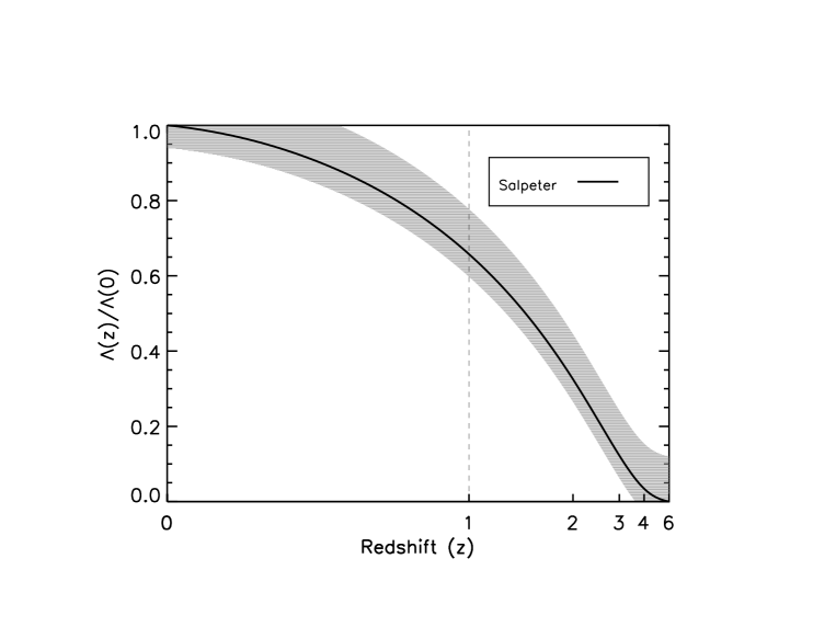
Figure 1: Normalized redshift evolution of the dark energy density, denoted by $\Lambda(z)$ and normalized to its present-day value $\Lambda(0)$. The shading in the figure represents the observational uncertainty in deriving the type II SNe rate, when a universal Salpeter initial mass function is adopted.

In Ref. 20 it is pointed out that, although $-w$ is close to unity, there is room for evolution during $z>0.5-1$. This is because the SNe Ia data only weakly constrain dark energy for such early times (there are still only a modest number of them detected). Furthermore, recent WMAP7 work³² provides limits on the properties of time dependent dark energy parameterized by

$$w(a)=w_{0}+w_{a}(1-a),$$ (34)

where $a$ is the scale factor of the universe ($a=\frac{1}{1+z}$), and $w_{0}=-0.93\pm 0.12$ with $w_{a}=-0.38^{+0.66}_{-0.65}$, for a flat cosmology.

The 13% uncertainty in $w_{0}$ is easily accommodated by the shading in Fig. (1), while the fiducial range of $w_{a}$ allows for a factor of 5 change in $\Lambda$ over $z=1-3$. Recent results by Ref. 33 yield $w_{0}=-0.905\pm 0.196$ and $w_{a}=-0.984^{+1.094}_{-1.097}$, which are again consistent with Fig. (1).

In any case, it is apparent that a modest improvement in future measurement precision of an effective $w$ around $z\sim 1$ could confirm or rule out the topological dynamics model for dark energy advocated here. Furthermore, the one-to-one correspondence between the number of macroscopic BHs and the dark energy density is very much open to astrophysical detection, given the accuracy with which the cosmic star formation history can be probed.²⁷ If verified, then this one-to-one link constitutes the proverbial smoking gun in support of the validity of the MP and the EMP.

5.3 The Spatial Scale and Timing of Dark Energy

The current value of the dark energy density $\Lambda$ is $\sim 10^{-29}$ g cm^-3.²⁹ Because $\Lambda=2N_{\rm BH}m_{P}/L_{f}^{3}$, the relation between the dark energy density and BH number can be used to compute $L_{f}$.

The present number of macroscopic (mostly stellar mass) BHs in the entire universe is approximately $N_{\rm BH}\sim 10^{19}$. From the present-day value of the dark energy density it then follows that $L_{f}\approx 2\times 10^{14}$ cm, about the size of the Solar system. Hence, the physical scale of the dark energy density, not specified in the topological dynamics studied here, is determined by empirical data. This renders the form of quantum gravity presented here fully fixed.

A number of other concerns regarding dark energy find a natural resolution when macroscopic BHs induce mini BHs. No modifications to matter degrees of freedom or additional (scalar) fields, like in quintessence as well as k-essence and Chaplygin gas approaches, are required or need to be justified in order to introduce dark energy.^34,35 In fact, because the star formation history of the universe sets the appearance of present-day dark energy, it is ultimately the Einstein equation itself that determines the evolution of $\Lambda$ (or some effective $w$).

Furthermore, since BHs are stellar remnants, it should come as no surprise that we witness dark energy in our time. Today is part of an epoch during which the bulk of the stars in the universe has been formed. This while the most massive of those stars have already exploded as SNe to leave behind BHs.

The change in the magnitude of the current dark energy density is set by the number of macroscopic BHs. With the bulk of all stars formed, so with much of the baryonic matter in galaxies turned into stars, this number cannot increase much further. We thus find ourselves, orbiting a typical star, close to the maximum dark energy density in time. This is for some value of $L_{f}$. The fact that the dark energy density is roughly comparable to the total matter density, in units of the critical density, then seems an odd coincidence.

However, a larger embedding volume $L_{f}^{3}$ for the universe diminishes $\Lambda$ as much as it increases the total mass in the universe available to make BHs. So $\Lambda$ is mostly affected by the mean mass of a BH as well as the fraction of baryonic matter that is converted into stars and subsequently into BHs. For the present universe these numbers are about a few Solar masses and 0.1%, respectively. Interestingly, stellar physics forbids much lower mass BHs because electron or neutron degeneracy pressure provides stability. A much larger BH mass or fraction would require a very exotic (and not observed) stellar initial mass function.

Hence, the value of $\Lambda\sim 10^{-29}$ g cm^-3 is a robust number, within 1-2 orders of magnitude, for an epoch after the peak in the cosmic star formation rate. This assumes that stellar remnants are the main source of long-lived BHs. The mean cosmic density, with its steep $(1+z)^{3}$ dependence, is currently about a few $\times 10^{-30}$ g cm^-3 and increases by orders of magnitude in the past. This while the universe has spend most of its cosmic life after the peak in the star formation history. This peak occurs for $z=1-2$, at least 9 billion years ago, but also billions of years after the big bang.

The densities of dark energy and matter are therefore roughly and naturally comparable for $z\sim 1-2$ if the bulk of the stars/BHs are in place. Also, we are likely to find ourselves after the peak in the cosmic star formation rate. The latter favors, through cosmic expansion, the dark energy density by a modest factor relative to the total matter density.

Hence, both the timing and magnitude of $\Lambda$ are as one would expect. An anthropic principle does not appear to be needed in any strong sense. Had the Earth been formed already a few billion years after the big bang, before the peak in the cosmic star formation history, then $N_{\rm BH}$ had simply not yet reached its maximum. Still, dark energy would not be completely absent either.

6 Inflation

The inflationary paradigm has shaped modern-day cosmology and knows many different incarnations.^{36,37,38,39,40} To further constrain topological dynamics, this section aims to link the solutions of the equation of motion above to a possible inflationary phase of the universe.

6.1 Number of e-Foldings and Present-Day Dark Energy

In the early universe, before the first long-lived BH stabilizes the quantum foam, Eq. (22) presents an exponential solution of the equation of motion for the handle multiplicity. Just like Wheeler’s stabilized quantum foam can be associated with dark energy, so can the young and unstable quantum foam be used to drive inflation.

For inflation to continue, so for Eq. (22) to pertain, it is necessary that the handle multiplicity is maintained. I.e., that the ambient matter and radiation density are high enough to suppress induced mini BH evaporation. The latter requires a detailed exploration of topologically extended GR. Such a study is postponed to a future paper. Nevertheless, if topological dynamics has any merit, then it is possible to compute the number of e-foldings during inflation from $L_{f}$, as follows.

The inflationary expansion of the universe is one of (infinitely) many homeomorphisms that space-time enjoys. Eq. (17) is invariant under homeomorphisms because of its topological nature (the MP). However, the form of Eq. (17) should also lead to the correct geometric limit because the longevity of macroscopic black holes yields the notion of a specific size scale $L_{f}$ (the EMP). Hence, one should seek a geometrization of Eq. (17).

At this point, the topologically void sub-equation of motion for $S^{3}$ actually becomes useful. Recall that

$$\Delta n_{2}S^{3}=\delta_{2}n_{2}S^{3}=0,$$ (35)

and consider topological time in the limit $m>>1$ and $\Delta m>>1$, written as $\tau$ for $m$ and $d\tau$ for $\Delta m<m$, during inflation. The value of $\Delta m$ need not be small when using the variable $\tau$. In physical units $\tau=mt_{P}>>t_{P}$, with an associated physical scale $R(\tau)=mt_{P}/c=ml_{P}$ (the same as $R(m)$). It is important to distinguish $\tau$ from geometric time $t$ here, because $2\Delta m<m$ does not hold for all $d\tau$. I.e., a priori, one considers all time intervals in the universe’s history.

One can now turn to the geometrization of Eq. (35). Although yielding a zero in terms of counting loops, geometrically one can represent the three-sphere by the relative size of the universe $S(\tau)$ for $n_{2}(m)\rightarrow S(\tau)$. That is, $S(\tau)$ measures the ratio (a dimensionless number) of the size of the universe with respect to its pre-inflationary state. Afterall, any notion of geometry on $S^{3}$, irrespective of a metric, should allow one to count Planck lengths if time is intrinsically discrete and if the speed of light $c$ is empirically found to be a universal constant.

The action of $\Delta$ is a first order time difference, which can now be written as $dS/d\tau$, for changes that are not necessarily small. The action of the counting operator $\delta_{2}$ only has meaning in conjunction with $n_{2}(m)\rightarrow S(\tau)$ and must yield $\delta_{2}S\rightarrow 0$ when one takes the limit $S\rightarrow\infty$. Therefore, $\delta_{2}$ must be representable as a function of $S$ alone and be a decreasing function thereof. Inflation is a homeomorphism that drives the universe to a flat state. The geometrization of $\delta_{2}$ thus represents vanishingly small curvature. Hence, $\delta_{2}\rightarrow 1/S^{2}$ and one finds that Eq. (35) turns into

$$\frac{dS}{d\tau}=\frac{1}{S}.$$ (36)

The solution $S(\tau)=(2\tau)^{1/2}$ is easily found. Because $\tau_{f}=L_{f}/l_{P}$ when $L_{f}$ becomes frozen in, one obtains $S_{f}=2^{1/2}(L_{f}/l_{P})^{1/2}$. Note that $L_{f}\approx 1.3\times 10^{47}$ in units of $l_{P}$, so that $S_{f}\approx 5.0\times 10^{23}$. One therefore finds that there is a natural correspondence. The pre-inflationary scaling law $R(t)\propto t^{1/2}$, for a local observer experiencing geometric time $t$, has the same form as the inflationary period scaling law $S(\tau)\propto\tau^{1/2}$, expressed in topological time $\tau$. This correspondence between $t$ and $\tau$ shows that a topologically driven inflationary period leads to a specific geometric embedding in 4-space for our universe.

It is good to realize here what the physical meaning of $\tau_{f}$ and $L_{f}$ is. The MP leads to the $L(T^{3})^{+}(m)$ structure of quantum space-time, which possesses a Lorentzian signature (see section 4.2). The large $m$ topological time $\tau$ then indicates a topological size $ml_{P}>>l_{P}$ on the lattice. Only when the first long-lived BH forms, can one speak of our universe as an entity of size $L_{f}$ that exists on $L(T^{3})^{+}$ with a distinct future $m^{\prime}>m_{f}=L_{f}/l_{P}$.

Since $L_{f}\propto N_{\rm BH}^{1/3}$ it follows that the increase in this characteristic size obeys $S_{f}\propto N_{\rm BH}^{1/6}$. This is a weak dependence. The number of e-foldings n scales as ${\rm n}\propto logN_{\rm BH}^{1/6}$ for $S_{f}\equiv e^{\rm n}$. The current value of $N_{\rm BH}\sim 10^{19}$ for stellar mass BHs in the observable universe yields ${\rm n}\approx 55$.

The stellar initial mass function in active galaxies or the early universe may have been top-heavy.⁴¹ Such a non-Salpeter shape favors high mass stars and can boost $N_{\rm BH}$ by easily an order of magnitude. Still, this will have a limited effect on n. Of course, the observable universe might be a lot smaller than the entire universe. Nevertheless, even a boost in $N_{\rm BH}$ by a factor of $10^{6}$ leads to an increase in n to $\approx 57$. In any case, these values are within the fiducial Planck range⁴² of 50-60.

6.2 The Onset of Inflation

A form of inflation that is driven by mini BHs suggests a start that picks up right after the big bang. However, this is not the case. First, one needs an ensemble of small BHs that are long-lived enough. In the sense that the mean lifetime of the ensemble is at least much larger than a Planck time. I.e., so that the handle multiplicity can at least be maintained, as already mentioned above. These BHs are referred to as longer-lived mini BHs.

The dark energy density is linearly proportional to the number of such longer-lived mini BHs, denoted as $N_{\rm BHll}$. Because $L_{f}$ is not yet frozen in at some time $mt_{P}<m_{f}t_{P}$, it is not obvious how to determine the specific volume $l^{3}$ for the dark energy density

$$\Lambda(m)=2N_{\rm BHll}\ m_{P}/l^{3}.$$ (37)

But, this characteristic length $l$ must be approximately set by the Schwarzschild radius $R_{\rm Sll}$ of the longest living mini BH, $l=R_{\rm Sll}$. The latter radius is the proper local length scale in topological dynamics. The number of Planck times $1<k<m$ in a BH’s existence is expressed through the number of three-tori. The longest living BH then sets $l$ because its life span comprises many more three-tori and their connections on $L(T^{3})^{+}(m)$ than do mini BHs with life times $k^{\prime}<k$.

Because $n_{0}(k)/n_{0}(k^{\prime})=7^{k-k^{\prime}}$, the longest living BH dominates the $L(T^{3})^{+}$ state space in terms of the information (entropy) required to describe it in 4-space. The longest living BH thus defines the most likely entropic state that the universe finds itself in. The precise number and characteristic mass of longer-lived mini BHs requires a full exploration of Eq. (17) within GR. Still, one can try to make an estimate of the typical longer-lived mini BH mass to obtain a grip on the timing of inflation.

Grand unified theory has a characteristic energy scale of $E_{c}\sim 10^{16}$ GeV, or about $\epsilon\sim 10^{-3}$ of the Planck energy. During this epoch, the universe has substantially cooled down in energy scale $E$ relative to the Planck energy, while primordial BH production may naturally occur during the associated phase transition. The thermodynamic temperature $T_{\rm BH}$ of a BH scales with its mass $m_{\rm BH}$ as $T_{\rm BH}\propto 1/m_{\rm BH}$, and thus its typical life time $t_{e}$ as $t_{e}\propto m_{\rm BH}^{3}$. It is therefore reasonable to estimate that one has longer-lived mini BHs with $m_{\rm BHll}\sim m_{P}/\epsilon$ that live for about $t_{e}\sim t_{P}/\epsilon^{3}\sim 10^{9}t_{P}$.

Consequently, one has a duration of at most $t_{e}$ to build up an ensemble of longer-lived mini BHs that can act as a base for inflation. Conversely, the size scale $R$ of the universe grows as $R\propto t^{1/2}$, so $t\propto R^{2}$, prior to inflation. It then takes a cool down period $t_{c}$ of about $t_{c}\sim t_{P}/\epsilon^{2}\sim 10^{6}t_{P}$ to reach the grand unification energy scale, since $E\propto 1/R$. In all, one expects inflation to commence after $t_{c}$ and before $t_{e}$. This yields a fiducial range of about $10^{6}-10^{9}t_{P}$. Although broad, the square root mean value is in line with general expectations.⁷

6.3 The Persistence of Homogeneity

There is also the issue of the initial conditions for inflation and how likely these are.⁴³ In units of $t_{P}$ a long time passes before mini BH driven inflation commenses. Over this time, some region of the vacuum that is to become inflated need not be in a state of homogeneity. If it has to be, then this renders the initial conditions quite unlikely.

However, the combination of the MP and the EMP form the topological heart of mini BH driven inflation. Together they dictate that every local Planckian volume responds, though the induction of Planckian mini BHs, in the same manner to the global ensemble of longer-lived mini BHs. This joint response prevents any strong inhomogeneity on scales larger than the Planck scale from occurring. The magnitude of fluctations on the Planck scale can be estimated as follows.

If the handle multiplicity is large, then the standard deviation of statistical fluctuations $\sigma$ decrease with $N_{\rm BHll}$ as $\sigma(m)=1/(2N_{\rm BHll}(m))^{1/2}$. Given the discrete nature of induced mini BHs, shot noise is the proper statistic for this phenomenon.

Also, the typical mass of a longer-lived mini BH was estimated above as $m_{\rm BHll}\sim 10^{3}m_{P}$, which yields $l\sim 10^{3}l_{P}$. Once the epoch of primordial longer-lived BH formation commences, $\Lambda(m)=2N_{\rm BHll}m_{P}/l^{3}$ is driven to the Planck energy density. This constitutes a form of topological reheating, because it is determined by the number of (quantum mechanically leaky) event horizons in the universe. It also implies that $N_{\rm BHll}\sim 10^{9}$ for $l\sim 10^{3}l_{P}$.

The latter number of $10^{9}$ should be close to the maximum value and thus set $\sigma$. An energy density on the order of the Planck density strongly suppresses the evaporation of induced mini BHs, thereby increasing the number of longer-lived BHs $N_{\rm BHll}$. However, the accretion rate of already existing longer-lived BHs would also be very high at the the Planck density. The latter boosts the mass of these BHs, and thus their longevity since $t_{e}\propto m_{\rm BH}^{3}$.

Hence, $N_{\rm BHll}\sim 10^{9}$ is not likely to grow much before a BH exists with a life span that exceeds the age of the universe at that time, thus freezing in the value of $L_{f}$. In all, one finds a very acceptable value of $\sigma\lesssim 2\times 10^{-5}$ for the magnitude of cosmological mass-energy fluctuations. Given that $N_{\rm BHll}(m)>>1$, the Poisson distribution of shot noise will typically be indistinguishable from Gaussian noise.

These perturbations are a result of the discrete nature of $\Lambda(m)$ and find their place in $T_{\mu\nu}$, so on the right hand side of the Einstein equation. Indeed, the very fact that GR relates geometry and matter allows one to include the global topological impact of dark energy as well as its local realization in energy-momentum.

6.4 Black Hole X: The End of Inflation

When $L_{f}$ is frozen in, this is locally determined by the favorable accretion history of one particular BH. However, $L_{f}$ is a global quantity. So if it is much larger than $l$, then the dark energy density drops very strongly and the universe exits inflation in a homogeneous (so-called graceful) manner. The actual size $l_{X}$ of the longer-lived mini BH $X$ that sets $L_{f}$ requires a detailed (numerical) computation. Nevertheless, a rough estimate of $l_{X}$ can be obtained.

Typically, $l\sim 10^{3}l_{P}$ while $t_{e}\propto m_{\rm BH}^{3}$ strongly depends on BH mass. Therefore, a relatively modest increase in the longer-lived mini BH mass likely suffices to freeze in $L_{f}$, given that the age of the universe at the onset of inflation is less than $\sim 10^{9}t_{P}$ and set by $t_{e}$. So, taking an excursion from the mean by a factor of 10, yields $m_{X}\sim 0.03$ g and an evaporation time $t_{X}\sim 10^{12}t_{P}$ for the first BH that lives longer than the age of the universe at that time.

Obviously, $l_{X}\sim 10^{4}l_{P}$ is very much smaller than the size $L_{f}$ of the universe at that time. In fact, $L_{f}/l_{X}\sim 10^{43}$ while $N_{\rm BHll}\sim 10^{9}$ during inflation and $N_{\rm BH}\sim 10^{19}$ today. Assuming that $l_{X}$ is an upper limit, this yields a ratio between the current dark energy density and the inflationary vacuum energy density of $\zeta\sim(N_{\rm BH}/N_{\rm BHll})(l_{X}/L_{f})^{3}\lesssim 10^{-119}$. This is approximately equal to the well known 120 orders of magnitude vacuum energy gap, and alleviates it through the MP and the EMP.

In all, the vacuum energy density at the end of the inflation diminishes globally by many orders of magnitude when BH X forms. This is a very desirable feature to match the very early universe energy scale with the current one. At the beginning of inflation the ambient radiation temperature was high and mini BH evaporation surpressed. The MP induces mini BHs every Planck time, providing fresh candidates. Combined this at least helps to build up a tail of (lucky) massive longer-lived BHs that can survive over cosmic times. That said, BH $X$ may not have lived to the present day. Still, that is irrelevant. BH $X$ is forever a part of the universe’s 4-space past.

6.5 The Scaling of Cosmological Perturbations

The longer-lived mini BHs are the driving force behind inflation in this work. Consequently, it is to be expected that the first and second order time derivative of $N_{\rm BHll}$ is small. Afterall, accretion does not affect BH number, while the evaporation time of these BHs is required to be at least on the order of the age of the universe in the first place. Because $N_{\rm BHll}$ acts as the single field here, there is thus a strong lack of rapidity in this type of inflation. The above fits the picture of slow-roll inflation.

The very nature of mini BH driven inflation avoids any problems with entropy generation (or reheating). In fact, the evaporation of induced mini BHs, in every Planckian volume, optimally uses (the second law of) thermodynamics at very large $T_{\rm BH}$. This while Eq. (22) supports an exponential dependence for $n_{1}(m)$ with topological time $m$. It is also good to recall the comments on $L_{f}$ and $\tau_{f}$ here, and to realize that our universe is properly embedded geometrically in 4-space only when BH $X$ forms and inflation ends. The latter can be pursued a bit further to also constrain the scaling of cosmological perturbations.

The induced mini BHs, denoted by $\Delta N$, appear in a quantum space-time $L(T^{3})^{+}$ that enjoys an exponentially rapid increase in geometric size $R(t)$. This picture introduces temporal effects, even when $N_{\rm BHll}$ is intrinsically constant, and can be used to determine the tensor-to-scalar ratio $r$ and the spectral index $n_{s}$, as follows.

Consider a local Planckian observer during inflation who is comoving with $R(t)$, so conformally, while $R(\tau)=l_{P}\tau$ measures the size of the universe in topological time $m>>1$ and $\Delta m>>1$, since the onset of inflation. Then $t\propto ln(R)\propto ln(\tau)$ and $dt=d\tau/\tau$. If $2\Delta m<m$ does not hold, then the coarse-grained nature of topological time affects the appearance of the induced mini BHs $\Delta N$ on $L(T^{3})^{+}$ because time slices $m$ are topologically identified over $\Delta m>>1$.

Under the assumption that the longer-lived BHs are local perturbations only, one has that $L(T^{3})^{+}\approx L(T^{3})$. The local Planckian observer, measuring for a geometric time interval $dt$ (not necessarily a small number), then notes the following. Induced mini BHs are spread out through time over intervals $dt>>t_{P}$. This generates very specific curvature perturbations. The observer sees mini BHs appear and disappear with a duty cycle that is set by the topological time $\tau$, for $\Delta m\rightarrow m$ and $\delta_{t}=1/m$ in $T^{3}|[R,\delta_{t}^{-1}]\in L(T^{3})$.

Furthermore, the scale invariance of these perturbations is broken because the duration $\tau$ of inflation sets a characteristic size $R(\tau)/l_{P}$ on $L(T^{3})$. So, even though $N_{\rm BHll}$ is constant, one has the situation that there is a gravitational wave generating quantity $r$ that should obey

$$r=\frac{dt}{t_{P}}\ \frac{d(\Delta N)}{d\tau}.$$ (38)

The observer concludes that there are ${\rm n}=\tau$ e-foldings ($\tau\rightarrow\tau+1$ stretches $t$ by a factor $e$) that diminish this tensor component during inflation. Indeed,

$$\frac{d(\Delta N)}{d\tau}=t_{P}\frac{d(\Delta N)}{\tau dt}\propto\frac{1}{{\rm n}}.$$ (39)

Also, every induced mini BH is attached to a heptaplet of three-tori on $L(T^{3})$ every $t_{P}$, driving its 7-fold topological identification across $\Delta m$. The observer counts these as 7 in his local geometric time frame, but $t\propto ln(\tau)$ and this yields $d(\Delta N)=ln(7)$. Hence, combined this gives $r=ln(7)/{\rm n}\approx 0.036$. According to the Planck results in Ref. 42, $r<0.11$ and one finds comfortable consistency.

In the constant $N_{\rm BHll}$ approximation, $r$ is fully driven by the distinction between topological and geometric time intervals. This while the spatial scaling properties of $T^{3}|[R,\delta_{t}^{-1}]\in L(T^{3})$ are completely expressed by the difference between $R(\tau)$ and $R(t)$, with the latter pertaining to our observational perspective. From above it also follows that $r\propto 1/\tau\propto 1/R(\tau)$, which is scale free.

So to find the relation between $r$ and $n_{s}$ one realizes that there is no fundamental topological distinction between $\tau$ and $R(\tau)$ or $t$ and $R(t)$. Any member of these two pairs can be taken as a temporal or spatial variable. Therefore, $r$ is equal to the relative amplitude of curvature perturbations ($\tau$ versus $t$) associated with mini BH induction on a dynamic $L(T^{3})$ background as well as to the deviation ($R(\tau)$ versus $R(t)$) from scale-free behavior of that $L(T^{3})$ background. Subsequently, $r$ and $n_{s}$ are equivalent and related by $n_{s}=1-r\approx 0.964$. This agrees very well with recent Planck observations⁴², which indicate $n_{s}=0.9603\pm 0.0073$.

In standard inflation theory, there is the subtle point of when modes cross the horizon. Such a phenomenon is not pertinent in inflation driven by topological dynamics. Rather, the Gaussian statistics of $T_{\mu\nu}$ in terms of $\sigma(m)$ are spatially uniform in a global manner thanks to the MP and EMP. With the additional numbers $n_{s}$ and $r$, the energy-momentum tensor has its properties fully specified.

7 Closing Remarks

7.1 Detecting the Topological to Geometric Time Transition

An additional route to explore the global character of our universe is to look for a macroscopic manifestation of the Planckian lattice of three-tori. The structure $L(T^{3})^{+}(m)$ is being build up further as we speak, rendering it exponentially more fine-grained spatially through Eq. (21). This precludes the occurrence of a multiply connected space-time on large spatial scales for cosmologically short time intervals. However, the transition of topological time $m$ to geometric time $t$ was described in section 4.2. The validity of the latter only holds for time intervals $\Delta m$ that obey $2\Delta m<m$.

An interesting situation then occurs for the cosmic microwave background (CMB). The current age of the universe is $t_{0}\approx 10^{61}t_{P}=m_{0}t_{P}$, about 14 billion years. The CMB has been travelling towards us since very close to that time, because the last scattering surface occurs only $\sim 10^{5.5}$ years after the big bang. Hence, geometric time is not a proper variable to describe topological dynamics cosmologically.

In particular, $L_{0}=ct_{0}$ is the largest scale that can be observed today, whatever the size $R(t_{0})>L_{0}$ of the universe. On $L_{0}$, the only observable constituent of $L(T^{3})^{+}$ is a pair of three-tori. For $2\Delta m\geq m_{0}$, the members of this pair are macroscopically separated and topologically identified on a scale $L_{0}/2$. Through this $T^{3}$ connection CMB radiation is temporally displaced over $t_{0}/2$. Because $L_{0}$ is what an observer perceives of the universe at $t_{0}$, geometric time only holds for scales $2L<L_{0}$. Note here that quantum space-time, so $L(T^{3})^{+}(m)$, is still continuous. It is our perception thereof that becomes crude.

This coarse-grained character of geometric time therefore leads to global spatial asymmetries in the CMB’s tiny temperature fluctuations. This topological redistribution process has some efficacy, which can be estimated as follows. As a consequence of the MP, each three-torus has a multiplication factor $F=1+\mu_{0}=7$, i.e., two heptaplets of three-tori perturb the CMB. Hence, some amount of radiation $U$ on the scale $L_{0}/2$ of one three-torus is temporally displaced across a scale $L_{0}/2$ to the other three-torus, and vice versa. One thus finds for the amplitude $B=dU/U$ of the resulting scalar fluctuation that

$$B=\frac{1}{2F}\approx 0.07.$$ (40)

Recent Planck data⁴⁴ indicate a large scale asymmetry with an amplitude of $B=0.07\pm 0.02$. This empirical value of $B$ is suggestively close to the theoretical prediction. Furthermore, the Planck data indicate multipole scales $\lambda\lesssim 60$. These correpond to spatial scales of $L_{0}-L_{0}/60$, fully consistent with $L_{0}/2$. This while such a $L(T^{3})^{+}$ driven asymmetry does not complicate the inflationary scenario discussed above.

Electromagnetic signals across time intervals $\Delta m<m_{0}/2$ experience no temporal displacement effects. But the early universe, roughly $z>0.6$ for more than 7 billion years ago, should also exhibit temporal displacement features. The distribution of luminous matter (e.g., galaxies) is the best place to look for these fluctuations. In a series of time slices through 4-space, they constitute a violation of the cosmological principle, driven by coarse-grained time as an expression of quantum space-time topology. Of course, the small amplitude $B$ of about 7% makes such temporal displacement fluctuations on a scale $L_{0}/2$ difficult to discern in an ensemble of large scale tracers.

7.2 Identification by Multiplication

Suppose the predictions on dark energy and inflation in this work are confirmed. Then quantum gravity, as a topological extension of GR in the form of Eq. (17), is an expression of the global multiply connected nature of Planckian space-time. In this, the EMP provides the link between the macroscopic and microscopic cosmos. Long-lived BHs induce mini BHs on the Planck scale, as miniature copies of the large scale originals.

The work presented here advocates the role of a very specific space-time topology for quantum gravity. In it, homeomorphically distinct paths in the form of loops take central stage and the prime manifolds $T^{3}$ and $S^{1}\times S^{2}$ express Feynman’s superposition and Wheeler’s quantum foam, respectively. The fundamental principle is the MP. The resulting quantum space-time is $L(T^{3})^{+}(m)$.

The MP dictates that the paths of quantum space-time are dynamical. Nature, so all observers combined, counts distinct paths unremittingly in order to identify them. Because it takes one to know one, a path that has been identified on the Planck scale must, in response to such observation, also have been multiplied as a part of quantum space-time. In all, the distinct paths that drive topological fluctuations on the Planck scale and underlie quantum gravity, obey a simple rule: multiply to identify.

Recall that Eq. (17) only appears simple. All the properties of Einstein gravity, as well as its possible modifications/unifications, are both part of and reduced to the complex temporal evolution of the number of quantum mechanically leaky event horizons on the Planck scale.

Overall, Eq. (17) has pertinent consequences for dark energy, inflation and the nature of time. A more complete exploration of the solutions to Eq. (17) may bring out new features for our cosmic evolution. In fact, such solutions can also help to test different modifications of GR against the observed history of our universe.

Topologically extended GR, expressed in discrete global time $m$ (through, e.g., a foliation based on BH longevity) and continuous intervals $(m+)=(m,m+1)$, is

$$G_{\mu\nu}[{\rm n}]+\Lambda_{A}(m)g_{\mu\nu}=8\pi GT_{\mu\nu}[n_{1}(m),\sigma(m)]_{r,n_{s}},$$ (41)

with $A=L_{f}$ or $A=R_{\rm Sll}$ (both generally covariant), $\Lambda(m)/m_{P}=2n_{1}(m)/A^{3}$ and $\sigma(m)=1/(2N_{\rm BHll}(m))^{1/2}$ the standard deviation of Gaussian mass-energy fluctuations induced by longer-lived BHs in the early universe, for ${\rm n}\approx 55$ e-foldings, $r=ln(7)/{\rm n}\approx 0.036$ and $n_{s}=1-r\approx 0.964$. In this,

$$n_{1}(m)[\{M_{k^{\prime}}\}]=n_{1}(m)[\{M_{k}\}]+2n_{1}(m)[m_{P}]+\Delta F(m+)-\Delta E(m+)-\Delta M(m+),$$ (42)

for the masses $M_{k}$ ($M_{k^{\prime}}$) that BHs $k=1...n_{1}(m)$ ($k^{\prime}=1...n_{1}(m+1)$) have, and for pairs of induced BHs with mass $m_{P}$. Periodic boundary conditions are imposed by the initial ($m=0$) three-torus that leads to $L(T^{3})$ and quantum superposition. To solve quantum gravity in the form of Eqs. (41) and (42) it is crucial that the evolution of the BH ensemble $n_{1}$ in $\Lambda$ and $T_{\mu\nu}$ is followed completely.

References

- [1] A. Einstein, Preuss. Akad. Wiss. Berlin Sitzber. (1915) 778.
- [2] A. Einstein, Letter to Arnold Ehrenfest on his discovery of GR (28 Nov. 1915).
- [3] J.A. Wheeler, Ann. of Phys. 2 (1957) 604.
- [4] J.A. Wheeler, Quantum Cosmology, eds. L.Z. Fang & R. Ruffini (World Scientific, 1987) p.27-92. This book provides a very nice overview of earlier developments in the field.
- [5] B.S. DeWitt, The Physical Review 160 (1967) 1587.
- [6] A. Ashtekar, Phys. Rev. D 36 (1987) 1587.
- [7] A. Ashtekar, Loop Quantum Gravity and the Planck Regime of Cosmology, arXiv:1303.4989 [gr-qc]. This paper contains many references to interesting works on loop quantum gravity cosmology.
- [8] S. Kaku, Introduction to Superstrings, 2nd edn. (Springer-Verlag, 1990).
- [9] R. Dijkgraaf and C. Vafa, Nuc. Phys. B 644 (2002) 3.
- [10] J.M. Maldacena, AdTMP 2 (1998) 231.
- [11] L. Smolin, General relativity as the equation of state of spin foam, arXiv:1205.5529 [gr-qc].
- [12] M. Spaans, Nuc. Phys. B 492 (1997) 526.
- [13] M. Spaans, J. Phys.: Conf. Ser. 410 (2013) 012149.
- [14] L. Smolin, The case for background independence, arXiv:hep-th/0507235.
- [15] S.W. Hawking, Comm. Math. Phys. 43 (1975) 199 as well as S.W. Hawking and D.N. Page, ApJ 206 (1976) 1.
- [16] K.S. Virbhadra and G.F.R. Ellis, Phys. Rev. D 65 (2002) 103004 as well as K.S. Virbhadra and C.R. Keeton, Phys. Rev. D 77 (2008) 124014
- [17] A.G. Riess et al., Astron. J 116 (1998) 116.
- [18] S. Perlmutter et al., ApJ 517 (1999) 565.
- [19] B.P. Schmidt et al., ApJ 507 (1998) 46.
- [20] R. Amanullah et al., ApJ 716 (2010) 712.
- [21] P.M. Garnavich et al. ApJ 509 (1998) 74.
- [22] R.P. Feynman, Rev. Mod. Phys. 20 (1948) 367.
- [23] M. Gromow and B. Larson, Publ. Math. 58 (1976) 295.
- [24] J. Hempel, 3-Manifolds; Annals of Mathematical Studies, Vol. 86 (Princeton, 1976).
- [25] M. Nakahara, Geometry, Topology and Physics, 1st edn. (Adam Hilger, 1990).
- [26] S. Dürr, T. Nonn and G. Rempe, Nature 395 (1998) 33.
- [27] A.M. Hopkins and J.F. Beacom 2006, ApJ 651 (2006) 142.
- [28] A. Aykutalp and M. Spaans, Testing the Proposed Connection between Dark Energy and Black Holes, arXiv:1201.6372 [astro-ph.CO].
- [29] G. Hinshaw et al., Nine-Year Wilkinson Microwave Anisotropy Probe (WMAP) Observations: Cosmological Parameter Results, arXiv:1212.5226 [astro-ph.CO].
- [30] P.A.R. Ade et al., Planck 2013 results. XVI. Cosmological parameters, arXiv:1303.5076 [astro-ph.CO].
- [31] R. Anantua, R. Easther and J.T. Giblin, Phys. Rev. Lett. 103 (2009) 111303.
- [32] E. Komatsu et al., ApJS 192 (2011) 18.
- [33] M. Sullivan et al. ApJ 737 (2011) 102.
- [34] K. Bamba, S. Capozziello, S. Nojiri and S.D. Odintsov, Astrophysics and Space Science 342 (2012) 155. Also, there is S. Tsujikawa, Quintessence: A Review, arXiv:1304.1961 [gr-qc]. These papers contain many references to different dark energy approaches.
- [35] S. Nojiri and S.D. Odintsov, Physics Reports 505 (2011) 59. Also, there is T.P. Sotiriou and V. Faraoni, Rev. Mod. Phys. 82 (2010) 451.
- [36] A.H. Guth, Phys. Rev. D 23 (1981) 347.
- [37] A.D. Linde, Phys. Lett. B 108 (1982) 389.
- [38] A. Albrecht and P.J. Steinhardt, Phys. Rev. Lett 48 (1982) 1220.
- [39] A.A. Starobinsky, Phys. Lett. B 91 (1980) 99.
- [40] A.A. Starobinsky, JETP Lett. 55 (1992) 489.
- [41] S. Hocuk and M. Spaans, A&A 536 (2011) A41.
- [42] P.A.R. Ade et al., Planck 2013 results. XII. Constraints on inflation, arXiv:1303.5082 [astro-ph.CO].
- [43] A. Ijjas, P.J. Steinhardt and A. Loeb, Inflationary paradigm in trouble after Planck2013, arXiv:1304.2785 [astro-ph.CO].
- [44] P.A.R. Ade et al., Planck 2013 results. XIII Isotropy and statistics of the CMB, arXiv:1303.5083 [astro-ph.CO].