Restoration of Quantum State in Dephasing Channel

Abstract

In this paper, we propose an explicit scheme to fully recover a multiple-qubit state subject to a phase damping noise. We establish the theoretical framework and the operational procedure to restore an unknown initial quantum state for an $N$-qubit model interacting with either individual baths or a common bath. We give an explicit construction of the random unitary (RU) Kraus decomposition for an $N$-qubit model interacting with a common bath. We also demonstrate how to use only one unitary reversal operation to restore an arbitrary state with phase damping noise. In principle, the initial state can always be recovered with a success probability of $1$. Interestingly, we found that non-RU decomposition can also be used to restore some particular entangled states. This may open a new path to restore a quantum state beyond the standard RU scheme.

I Introduction

Recent research has focused on protection or restoration of a quantum state subject to the influence of intrinsic and extrinsic noises Book1 ; Book2 ; QCQI . Quantum noise is ubiquitous and is typically registered as disentanglement and loss of quantum coherence WW ; XX ; YY ; Yu-Eberly04 . Several theoretical schemes have been proposed to control decoherence, ranging from dynamic decoupling control DD and feedback control FBC , to weak measurement WK1 ; WK2 ; WK3 and error correction codes ECC , etc. While the dynamic decoupling and weak measurement are implemented to protect the quantum states by active external interventions, the error correction in quantum codes can be achieved through a passive realization of the encoded systems. However, in all realistic applications, the errors in quantum operations utilized in quantum information processing cannot be completely eliminated. Besides, the intricacy in manipulating coupled multiple-qubit systems has posed a serious challenge in scalable realizations in various quantum information carriers. All these fundamental issues of decoherence and control are still active research subjects.

Quantum decoherence can be modeled as a non-unitary process, and the non-unitary dynamics of a quantum open system can be described by a master equation. Clearly, a state evolving unitarily in an ideally closed system can be recovered by one unitary reversal operation. Therefore it is natural to ask, is it possible to recover an initial quantum state for a non-unitary evolution via a unitary quantum reversal operation?

The state of an quantum open system, denoted by the reduced density operator $\rho_{S}$ at time $t$, may be written in the form of Kraus (operator sum) representation Choi ; Lind ; Kraus ; QCQI : $\rho_{S}(t)={\textstyle\sum_{n}}K_{n}(t)\rho_{S}(0)K_{n}^{\dagger}(t)$ with $\sum_{n}K_{n}^{\dagger}K_{n}=I$. If these Kraus operators $K_{n}$ are proportional to a set of unitary operators as $K_{n}=c_{n}U_{n}$, then restoration of the initial quantum state is possible LostFound , and such a decomposition is called a random unitary (RU) decomposition with RU-type Kraus operators $\{K_{n}\}$. In a well-defined situation where the environment is measurable, M. Gregoratti and R. F. Werner explicitly provide an error correction scheme which needs only one reversal operation on the system based on the outcome of a measurement performed on the environment LostFound . Ideally, the success probability is always $1$, and the fidelity of the recovered state is also $1$. This restoration scheme is of interest in many scenarios where a quantum measurement may be performed on the environment under consideration. However, generally it is not clear whether or not the required RU decomposition always exists. In fact, it has been shown that the RU decomposition does not exist in a generic dissipative model EC_dissipative . Even in cases for which it does exist, finding the RU-type Kraus operators is often difficult. For the dephasing channel, Buscemi et al. prove that if the dimension $d$ of the Hilbert space satisfies $d\leqslant 3$, then the RU decomposition does always exist Buscemi2 . Moreover, Strunz and co-workers have provided an explicit example of the RU decomposition for the one-qubit dephasing channel Strunz . However, the explicit construction of an RU decomposition for an $N$-qubit system coupled to a general environment has not yet been proposed.

The purpose of this paper is to explicitly construct an RU decomposition for an $N$-qubit model in both the individual baths case and the common bath case. We investigate the feasibility of performing environment-assisted error correction for dephasing chanel. Since a major limitation of the original scheme LostFound is that RU decomposition rarely exists for certain models, we provide an example of how to use non-RU decomposition to fully recover some entangled states, and thus overcome the RU limitation. Moreover, in our scheme, the measurement performed on the environment is in the Fock basis, the restoration, in many interesting cases, only depends on the parity of total photon numbers (even or odd) in the environment. This may enhance the feasibility of experimental realizations of the proposed restoration scheme.

This paper is organized as follows: in Sec. II, we review the general error correction scheme proposed in LostFound and developed in EC_Depolarizing ; EC_dissipative ; Buscemi1 ; Buscemi2 ; Strunz ; Audenaert2008 ; Rosgen2008 ; Hayden2005 ; Lidar2010 ; Exp_ECC . In Sec. III, we investigate the case of an $N$-qubit model interacting with a common bath. Particularly, we explicitly construct the RU decomposition and non-RU decomposition for this $N$-qubit system. When the RU decomposition exists, the initial state may be recovered using the standard restoration scheme. Interestingly, our work goes beyond the standard restoration scheme based on the RU decomposition LostFound . We show that, for a non-RU decomposition, a quantum operation can entail a full recovery of some entangled states embedded in the phase noise. In Sec. IV, we investigate another type of interaction between system and baths, $N$ qubits interacting with individual baths. We first derive the RU-type Kraus decomposition for a single-qubit system associated with an explicit measurement basis. Then, we extend the restoration scheme to the $N$-qubit model interacting with individual dephasing baths. Thus, we show that perfect restoration can always be achieved for a multiple-qubit system for both the common bath case and the individual baths case.

II Error Correction Scheme Based on RU Decomposition

The framework of open quantum systems is established from quantum theory for the total system (system plus environment), which is governed by the Schrödinger equation. The evolution of the total density matrix is given by $\rho_{{\rm tot}}(t)=U\rho(0)U^{\dagger}$, where $U=e^{-iH_{{\rm tot}}t}$ (setting $\hbar=1$) is the total evolution operator. The evolution for the reduced density matrix of the system can be obtained by tracing over the environmental degrees of freedom $\rho_{S}(t)=\text{tr}_{E}[\rho_{{\rm tot}}(t)]$, and it can formally be written in the Kraus (operator sum) representation Choi ; Kraus ; QCQI ; Lind ,

$$\rho_{S}(t)={\textstyle\sum_{n}}\langle n|U|0\rangle\rho_{S}(0)\langle 0|U^{\dagger}|n\rangle={\textstyle\sum_{n}}K_{n}\rho_{S}(0)K_{n}^{\dagger},$$ (1)

where $K_{n}=\langle n|U|0\rangle$ are the so-called Kraus operators, which depend on the initial state of the environment and the choice of the complete basis of the environment $\{|n\rangle\}$. Changing the basis of the environment from $\{|n\rangle\}$ to $\{|m\rangle\}$ as $\langle n|=\sum_{m}\langle m|V_{n,m}$ will lead to another set of Kraus operators $L_{m}=\langle m|U|0\rangle$, where $V$ is a unitary matrix and the relation between the two sets of Kraus operators can be written as

$$K_{n}={\textstyle\sum_{m}}V_{n,m}\langle m|U|0\rangle={\textstyle\sum_{m}}V_{n,m}L_{m}.$$ (2)

Clearly, a measurement on the environment will collapse the environment into an eigenstate of the measured observable. Correspondingly, the system will also be projected into a state relative to each resultant environmental state after measurement, i.e., $\rho_{S,n}(t)=K_{n}\rho_{S}(0)K_{n}^{\dagger}$, if we observe the $n^{\text{th}}$ outcome in the measurement of environment. Equation (1) represents an ensemble of the system states without specifying the measurement outcomes. If the decomposition (1) is RU, i.e., $K_{n}=c_{n}U_{n}$ for each $n$, where $U_{n}^{\dagger}=U_{n}^{-1}$ and $c_{n}$ satisfy $\sum_{n}|c_{n}|^{2}=1$, one can apply an inverse operation to recover the initial quantum state based on the measurement outcome $n$,

$$\rho_{R}(t)=R_{n}\rho_{S,n}(t)R_{n}^{\dagger}=\rho_{S}(0),$$ (3)

where $R_{n}=\frac{1}{c_{n}}U_{n}^{-1}$. This scheme of restoring initial quantum states depends on the form of the Kraus decomposition. If an RU-type Kraus decomposition exists, the quantum information stored in the initial state can be fully recovered.

III $N$ Qubits in a Common Bath

Focusing on the dephasing channel YuPRB ; Liu , the simplest example, the single-qubit case, has been analyzed in Ref. Strunz , where an RU decomposition is constructed. Here, we will start from the model of two qubits in a common bath and then extend the method to a general $N$-qubit case. The single-qubit case can be revealed as a special case in our framework. In the discussion in subsection IV.2, we will see the measurement required in our method is based on Fock states, which is much simpler than the method discussed in Ref. Strunz .

III.1 Two-Qubit Non-RU Decomposition and Entanglement Restoration

It is instructive to consider first how to recover a quantum entangled state via a non-RU decomposition, while the restoration of arbitrary initial states based on RU decomposition will be discussed later. For the common bath case, the Hamiltonian of the two-qubit dephasing model is $H=\frac{\omega}{2}S_{z}+\sum_{k}\omega_{k}b_{k}^{\dagger}b_{k}+\sum_{k}g_{k}S_{z}(b_{k}+b_{k}^{\dagger})$, where $S_{z}=\frac{1}{2}(\sigma_{z}^{A}+\sigma_{z}^{B})$. Assuming the initial state of environment is the vacuum state $|0\rangle$, in the interaction picture, the solution of the Schrödinger equation is $|\psi_{tot}(t)\rangle=U|\psi_{S}(0)\rangle|0\rangle$, where

$$U=\prod_{k}e^{-i\phi_{k}(t)S_{z}^{2}}e^{-iS_{z}b_{k}^{\dagger}G_{k}(t)}e^{-iS_{z}b_{k}G_{k}^{*}(t)},$$ (4)

where $G_{k}(t)=\int_{0}^{t}g_{k}e^{i\omega_{k}s}ds$, and $\frac{d}{dt}\phi_{k}(t)=-ig_{k}e^{-i\omega_{k}t}G_{k}(t)$. Then,

$$\langle\{m_{k}\}|U|0\rangle=\prod_{k}e^{-i\phi_{k}(t)S_{z}^{2}}\frac{[-iS_{z}G_{k}(t)]^{m_{k}}}{m_{k}!}$$ (5)

where the notation $|\{m_{k}\}\rangle\equiv|m_{1},m_{2},m_{3}\cdots\rangle\equiv\otimes_{k}|m_{k}\rangle$ represents the multi-mode Fock state, where $m_{k}$ are photon numbers in the $k^{\text{th}}$ mode. In (5), every excitation in the environment contributes one $S_{z}$ operator, so the product contains $(S_{z})^{m}$ operators ($m=\sum_{k}m_{k}$ is the total photon number). If the total photon number $m$ is odd, we have $(S_{z})^{m}=S_{z}$; if the total photon number $m$ is even, we have $(S_{z})^{m}=S_{z}^{2}$; if all the $m_{k}$ are zero, only the first term $e^{-i\phi_{k}(t)S_{z}^{2}}$ is left. Finally, we have only three types of Kraus operators:

1. If $|\{m_{k}\}\rangle=|0\rangle$, then

$$\langle\{m_{k}\}|U|0\rangle=\text{diag}\{l_{1}(t),1,1,l_{1}(t)\},$$ (6)

where the time-dependent element is

$$l_{1}(t)=\exp[-\int_{0}^{t}dt^{\prime}\int_{0}^{t^{\prime}}\alpha(t^{\prime},s)ds],$$ (7)

with $\alpha(t^{\prime},s)=\sum_{k}g_{k}^{2}e^{-i\omega_{k}(t^{\prime}-s)}$.

2. If the total photon number $m\equiv\sum\nolimits_{k}m_{k}$ in $|\{m_{k}\}\rangle$ is odd, then

$$\langle\{m_{k}\}|U|0\rangle=F_{\{m_{k}\}}^{odd}(t)S_{z},$$ (8)

where $F_{\{m_{k}\}}^{odd}=\prod_{k}e^{-i\phi_{k}(t)}\frac{[-iG_{k}(t)]^{m_{k}}}{m_{k}!}$.

3. If the total photon number $m\equiv\sum\nolimits_{k}m_{k}$ in $|\{m_{k}\}\rangle$ is even but not $0$, then

$$\langle\{m_{k}\}|U|0\rangle=F_{\{m_{k}\}}^{even}(t)S_{z}^{2},$$ (9)

where $F_{\{m_{k}\}}^{even}=\prod_{k}e^{-i\phi_{k}(t)}\frac{[-iG_{k}(t)]^{m_{k}}}{m_{k}!}$.

The reduced density matrix can be recovered by these three types of Kraus operators as

$$\rho_{S}(t) = {\textstyle\sum_{\{m_{k}\}}}\langle\{m_{k}\}|U|0\rangle\rho_{S}(0)\langle 0|U^{\dagger}|\{m_{k}\}\rangle$$ (10)

$$= \langle 0|U|0\rangle\rho_{S}(0)\langle 0|U^{\dagger}|0\rangle$$

$$+{\textstyle\sum_{\{m_{k}\}}^{m=odd}}\langle\{m_{k}\}|U|0\rangle\rho_{S}(0)\langle 0|U^{\dagger}|\{m_{k}\}\rangle$$

$$+{\textstyle\sum_{\{m_{k}\}}^{m=even}}\langle\{m_{k}\}|U|0\rangle\rho_{S}(0)\langle 0|U^{\dagger}|\{m_{k}\}\rangle$$

$$= \langle 0|U|0\rangle\rho_{S}(0)\langle 0|U^{\dagger}|0\rangle$$

$$+{\textstyle\sum_{\{m_{k}\}}^{m=odd}}|F_{\{m_{k}\}}^{odd}|^{2}S_{z}\rho_{S}(0)S_{z}$$

$$+{\textstyle\sum_{\{m_{k}\}}^{m=even}}|F_{\{m_{k}\}}^{even}|^{2}S_{z}^{2}\rho_{S}(0)S_{z}^{2}$$

$$= {\textstyle\sum_{i=1}^{3}}L_{C,i}\rho_{S}(0)L_{C,i}^{\dagger}.$$

In the matrix form, these non-RU-type Kraus operators $L_{C,i}$ can be explicitly written as:

$$L_{C,1} = \text{diag}\{l_{1}(t),1,1,l_{1}(t)\},$$ (11)

$$L_{C,2} = l_{2}(t)\text{diag}\{1,0,0,-1\},$$ (12)

$$L_{C,3} = l_{3}(t)\text{diag}\{1,0,0,1\},$$ (13)

corresponding to the vacuum state, odd state, and even state, respectively. The time-dependent coefficients can be expressed as $l_{1}(t)=\!\exp[-\int_{0}^{t}dt^{\prime}\int_{0}^{t^{\prime}}\alpha(t^{\prime},s)ds]$, $l_{2}(t)=\sqrt{{\textstyle\sum_{\{m_{k}\}}}|F_{\{m_{k}\}}^{odd}|^{2}}$, and $l_{3}(t)=\sqrt{{\textstyle\sum_{\{m_{k}\}}}|F_{\{m_{k}\}}^{even}|^{2}}$.

The corresponding measurement operators for this set of Kraus operators are $M_{C,1}=|0\rangle\langle 0|$, $M_{C,2}=\sum_{\{m_{k}\}}^{m=odd}|\{m_{k}\}\rangle\langle\{m_{k}\}|$, and $M_{C,3}=\sum_{\{m_{k}\}}^{m=even}|\{m_{k}\}\rangle\langle\{m_{k}\}|$, where $m$ is the total photon number summed over all modes. They satisfy $M_{C,i}M_{C,j}=\delta_{i,j}M_{C,i}$, $\sum_{i=1}^{3}M_{C,i}=I$, and $M_{C,i}$ are all non-negative. Performing a measurement on this set of measurement operators, the possible outcomes give the non-RU decomposition as

$$\text{tr}_{E}[U\rho(0)U^{\dagger}M_{C,i}]=L_{C,i}\rho_{S}(0)L_{C,i}^{\dagger},\;(i=1,2,3)$$ (14)

with probability $p_{C,i}=\text{tr}[L_{C,i}\rho_{S}(0)L_{C,i}^{\dagger}]$.

This set of Kraus operators $L_{C,i}$ are obviously non-RU-type. We show below that one can exploit the non-RU decomposition to recover quantum entangled states. Then the restoration based on this set of non-RU Kraus operators goes beyond the standard scheme LostFound . Consider two major types of initially entangled states $|\Phi\rangle=\alpha|00\rangle\pm\beta|11\rangle$ and $|\Psi\rangle=\alpha|01\rangle\pm\beta|10\rangle$, where $|\alpha|^{2}+|\beta|^{2}=1$. The second one is decoherence-free in passage through the channel (10), so we only focus on the first type, $|\Phi\rangle$. For this type of initial states, the restoration operators are $R_{C,1}=l_{1}^{-1}\text{diag}\{1,1,1,1\}$, $R_{C,2}=l_{2}^{-1}\text{diag}\{1,1,1,-1\}$, and $R_{C,3}=l_{3}^{-1}\text{diag}\{1,1,1,1\}$, which are unitary operations. It is easy to check that

$$R_{C,i}L_{C,i}|\Phi\rangle\langle\Phi|L_{C,i}^{\dagger}R_{C,i}^{\dagger}=|\Phi\rangle\langle\Phi|,\;(i=1,2,3)$$ (15)

meaning that the restoration operations give back the unknown initial state precisely in all possible outcome scenarios. The experimental setup is just measuring the environment in the Fock basis, and based on the results $M_{C,1}$ ($|0\rangle$ state), $M_{C,2}$ (odd state), or $M_{C,3}$ (even state), we perform the corresponding restoration operations $R_{C,1}$, $R_{C,2}$, or $R_{C,3}$. The restoration procedure is explicitly shown in Fig. 1.

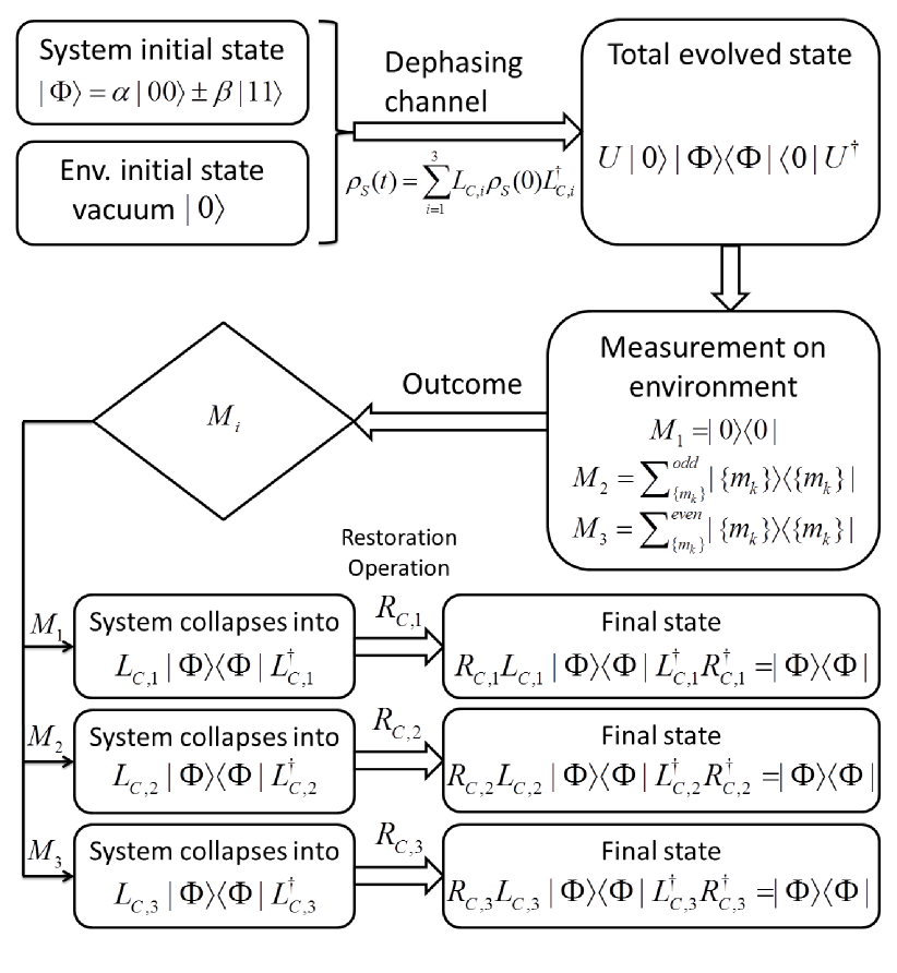
Figure 1: Entangled states restoration scheme.

Although this scheme is only applicable to some particular initial states, the experimental setup will be relatively easy since the measurement basis is just the Fock states separated into families based on parity. Besides, in most quantum information processing schemes, entangled states like $|\Phi\rangle$ and $|\Psi\rangle$ are the most commonly used initial states. Now, we treat the case of arbitrary initial states, and then compare these two schemes.

III.2 Two-Qubit RU Decomposition

In order to construct an RU decomposition and deal with arbitrary initial states, we need to find another set of RU-type Kraus operators which are linear combinations of the $L_{C,i}$. Consider the following ansatz:

Suppose the RU-type Kraus operators have the form

$$K_{C,1} = \sqrt{x_{1}}\text{diag}\{1,1,1,1\},$$ (16)

$$K_{C,2} = \sqrt{x_{2}}\text{diag}\{-1,1,1,1\},$$ (17)

$$K_{C,3} = \sqrt{x_{3}}\text{diag}\{1,1,1,-1\},$$ (18)

$$K_{C,4} = \sqrt{x_{4}}\text{diag}\{1,-1,-1,1\}.$$ (19)

Then, using the relation

$$\rho_{S}(t)={\textstyle\sum_{i=1}^{3}}L_{C,i}\rho_{S}(0)L_{C,i}^{\dagger}={\textstyle\sum_{j=1}^{4}}K_{C,j}\rho_{S}(0)K_{C,j}^{\dagger},$$ (20)

the coefficients $x_{j}$ $(j=1,2,3,4)$ are determined as

$$x_{1} = \frac{1}{4}(1+2l_{1}+|l_{3}|^{2}-|l_{2}|^{2}),$$ (21)

$$x_{2} = x_{3}=\frac{1}{4}(1-|l_{3}|^{2}+|l_{2}|^{2}),$$ (22)

$$x_{4} = \frac{1}{4}(1-2l_{1}+|l_{3}|^{2}-|l_{2}|^{2}).$$ (23)

Since the $K_{C,i}$ are all RU-type Kraus operators, then their inverse operations $R_{C,i}$ as in (3) always exist.

Finding the RU-type Kraus decomposition only proves the feasibility of perfect restoration of the initial state. In practice, we still need to find the measurement operators corresponding to the RU-type Kraus operators. It is well-known that any two Kraus decompositions of the same quantum channel must be connected by a unitary matrix QCQI ; Strunz , as in (2). The simplest Kraus decomposition is given by $L_{\{m_{k}\}}^{\prime}=\langle\{m_{k}\}|U|0\rangle$ where we have infinite numbers of Kraus operators $L_{\{m_{k}\}}^{\prime}$ since we choose the Fock basis $\{|m_{k}\rangle\}$. Then we can follow the scheme in Strunz to give the measurement basis for the $K_{C,i}$. The unitary transition matrix is just the one connecting $K_{C,i}$ and $L_{\{m_{k}\}}^{\prime}$. Although there are infinite numbers of $L_{\{m_{k}\}}^{\prime}$, we will show that only the first several $L_{\{m_{k}\}}^{\prime}$ operators are non-zero so that we can set a cutoff and find the transition matrix by simply solving a set of linear equations.

For simplicity, we use the single-mode case as an example. For a single-mode environment, the simplest $m$ Kraus operators (for a harmonic oscillator, $m$ goes from $0$ to $\infty$), can be expressed as $L_{m}^{\prime}=\langle m|U|0\rangle$, and the density matrix is

$$\rho_{S}(t) = {\textstyle\sum_{m=0}^{\infty}}\langle m|U|0\rangle\rho_{S}(0)\langle 0|U^{\dagger}|m\rangle$$ (24)

$$= {\textstyle\sum_{m=0}^{\infty}}L_{m}^{\prime}\rho_{S}(0)L_{m}^{\prime}{}^{\dagger}.$$

Each Kraus operator $L_{m}^{\prime}$ can be determined by (5) or computed directly by numerical methods. Meanwhile, we have also derived another set of RU-type Kraus operators in (16-19), since the two sets of Kraus operators must be connected by a unitary matrix $V$ as

$$K_{C,n}={\textstyle\sum_{m=1}^{\infty}}V_{n,m}L_{m-1}^{\prime},$$ (25)

where in the case that $n>4$, $K_{C,n}$ are all zero. Then, writing the equation in matrix form, it becomes

$$\left[\begin{array}[]{c}K_{C,n}(1,1)\\ K_{C,n}(2,2)\\ K_{C,n}(3,3)\\ K_{C,n}(4,4)\end{array}\right]=\left[\begin{array}[]{ccc}L_{0}^{\prime}(1,1)&\cdots&L_{m-1}^{\prime}(1,1)\\ L_{0}^{\prime}(2,2)&\cdots&L_{m-1}^{\prime}(2,2)\\ L_{0}^{\prime}(3,3)&\cdots&L_{m-1}^{\prime}(3,3)\\ L_{0}^{\prime}(4,4)&\cdots&L_{m-1}^{\prime}(4,4)\end{array}\right]\!\left[\begin{array}[]{c}V_{n,1}\\ V_{n,2}\\ \vdots\\ V_{n,m}\end{array}\right]\!,$$ (26)

where the numbers in parentheses indicate matrix elements and the coefficient matrix is a $4\times m$ matrix. Although the matrix is infinite-dimensional, the probability to find a high-excitation state $|m\rangle$ (i.e. a very large $m$) in the environment is actually very small. According to (5), when the total excitation $m$ is large, $L_{m}^{\prime}=\langle m|U|0\rangle$ is close to zero. Therefore, we can take a cutoff when solving (26).

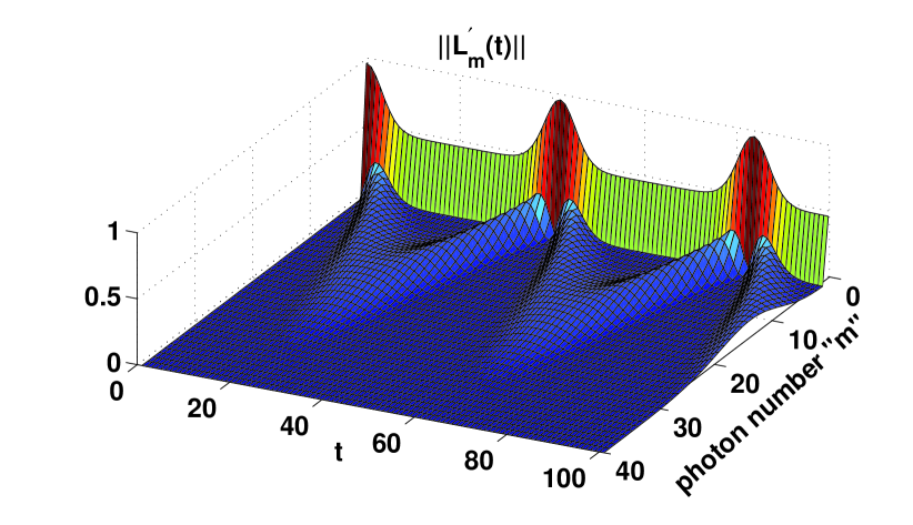
Figure 2: (color online) $||L_{m}^{\prime}(t)||$ vs $t$ and $m$.

We numerically verify this in Fig. 2, in which we can see that when the photon number is large, the trace norm ($||A||\equiv\text{tr}[\sqrt{A^{\dagger}A}]$) of the Kraus operators $L_{m}^{\prime}(t)$ is always close to zero. Therefore, it is safe to drop the high excitation states and the coefficient matrix becomes finite-dimensional. For example, according to Fig. 2, we can safely choose $L_{m-1}^{\prime}=0$ when $m>30$, so then the coefficients matrix is $4\times 30$. Therefore, the equations for $V$ form a set of first order linear equations. Since all the $L_{m-1}^{\prime}$ are known, i.e. the coefficient matrix is fully determined, it can be solved by computer rather quickly.

Finally, the measurement basis is just

$$|\psi_{n}\rangle={\textstyle\sum_{m=1}^{30}}V_{n,m}^{*}|m\rangle,\quad(m,n=1,\ldots,30).$$ (27)

The first four measurement basis states $|\psi_{n}\rangle$ ($n=1,2,3,4$) just correspond to RU-type Kraus operators $K_{C,n}$, and the probabilities of finding the other measurement outcomes $|\psi_{n}\rangle$ ($n>4$) are zero Strunz .

Although the measurement basis states for RU decomposition can be easily numerically determined by the procedure above, the physical meaning is still unclear since they are superpositions of Fock states, and more importantly, it may be difficult to perform such measurements.

In the common bath case, the Fock basis does not admit an RU decomposition. To overcome this, we have two options. The first option is to construct an RU decomposition with Kraus operators $K_{C,i}$, which will shift the difficulty to finding the measurement operators. Unfortunately, such measurement operators are difficult to realize. However, if we can overcome this by cleverly designing an experimental measurement procedure, then the advantage of this first choice is that the restoration scheme is applicable to arbitrary initial states.

On the other hand, the second option is that we can make a compromise about what we choose for the initial states. If we are only interested in recovering some particular unknown entangled states (and in most quantum information processing schemes, the initial states are usually the entangled states we discussed), then we can go beyond the RU decomposition scheme.

The non-RU decomposition may give us a much simpler way of recovering entangled states, and simplify the implementation of the measurements. Based on our current knowledge of experimental techniques, we show the whole scheme of the second option, and theoretically prove the feasibility of the first option. Then, we leave the problem of designing a clever experiment to perform a measurement on superposition Fock states to future investigations.

III.3 RU Decomposition for the $N$-Qubit Case

Using the technique of constructing RU Kraus decomposition for the two-qubit case, we can try to solve the general $N$-qubit case. Therefore, to gain some insight, we will explicitly construct the RU decomposition of the three-qubit case as a special example. First, we will review some properties of the dephasing channel which have been studied in Jing-Yu . According to Jing-Yu , the $N$-qubit dephasing channel can be expressed as

$$\rho_{S}(t)=C(N)\circ\rho_{S}(0),$$ (28)

where $A\circ B$ is the entry-wise product of matrices $A$ and $B$ (also called a Schur or Hadamard product). Although the dimension of matrix $C(N)$ is $N^{2}$, the rank $C(N)$ is

$$R(N)=\text{rank}[C(N)]=N+1,$$ (29)

i.e. only $R(N)$ rows or columns give us useful information. Therefore we can always shift the linearly independent rows (columns) to the top-left of the whole matrix, in which case it takes the form,

$$C(N)\Rightarrow\left[\begin{array}[]{cc}M&M^{\prime}\\ M^{\prime}&M^{\prime\prime}\end{array}\right],$$ (30)

where $M$ is the linearly independent part ($\text{dim}(M)\!=\!\text{rank}[C(N)]\!=\!N+1$) while $M^{\prime}$ and $M^{\prime\prime}$ are linearly dependent parts. Moreover, the matrix elements of $C(N)$ only contain $\{\gamma^{0}(t),\gamma^{1^{2}}(t),\gamma^{2^{2}}(t),\cdots,\gamma^{(N-1)^{2}}(t),\gamma^{N^{2}}(t)\}$, where $\gamma(t)$ describes the decay of off-diagonal elements. The elements in $M$ are $\gamma^{N^{2}}$ to $\gamma^{0}$, sweeping in diagonal groups anti-diagonally from the top-right to the main-diagonal elements Jing-Yu , so that

$$M=\left[\begin{array}[]{cccc}1&\cdots&\gamma^{(N-1)^{2}}&\gamma^{N^{2}}\\ \vdots&1&\cdots&\gamma^{(N-1)^{2}}\\ \gamma^{(N-1)^{2}}&\cdots&1&\vdots\\ \gamma^{N^{2}}&\gamma^{(N-1)^{2}}&\cdots&1\end{array}\right].$$ (31)

Given these facts, the following procedure shows how to construct the RU decomposition for an arbitrary $N$-qubit dephasing channel.

First, write down the Schur matrix $C(N)$ of the channel, and delete the rows (columns) which are not linearly independent. Then, we can choose $N_{K}$ (we will give this number below) basis operators $\{B_{1},\cdots,B_{N_{K}}\}$ which are all diagonal matrices in which the diagonal elements are either $1$ or $-1$, e.g.,

$$B_{1}=\text{diag}\{1,1,\cdots,1\},\quad B_{N_{K}}=\text{diag}\{1,-1,\cdots,-1\}.$$ (32)

Given this basis, the RU-type Kraus operators are

$$K_{i}=\sqrt{c_{i}}B_{i}\quad(i=1,\cdots,N_{K}),$$ (33)

where $c_{i}$ are coefficients which can be determined by

$${\textstyle\sum_{i=1}^{N_{K}}}K_{i}\rho_{S}(0)K_{i}^{\dagger}=C(N)\circ\rho_{S}(0).$$ (34)

Next, determine how many (i.e., the number $N_{K}$) basis operators are needed for the RU decomposition. In $C(N)$, only $M$ is useful while $M^{\prime}$ and $M^{\prime\prime}$ contain no new information. Thus, the number of independent equations in (34) is just the number of the upper triangular elements in $M$ plus one, i.e.,

$$N_{K}=1+{\textstyle\sum_{k=1}^{N}}k=1+\frac{N(N+1)}{2},$$ (35)

since $M$ is $(N+1)\times(N+1)$. That is the reason we need to choose $N_{K}$ basis elements; we need $N_{K}$ coefficients $c_{i}$ to satisfy those equations given by (34). Solving for the coefficients $c_{i}$ $(i=1,\cdots,N_{K})$ and substituting them back into (33), all the Kraus operators for the RU decomposition of our $N$-qubit dephasing channel are fully determined. There are a total of $2^{2^{N}}$ choices of basis, but we only need $N_{K}=1+\frac{N(N+1)}{2}$ basis elements, so the choice of basis is not unique.

It will be helpful to understand the above scheme of constructing the RU decomposition of the $N$-qubit model by explicitly solving the three-qubit case as an example. In the three-qubit case, the matrix $C(3)$ is

$$C(3)=\left[\begin{array}[]{cccccccc}1&\gamma&\gamma&\gamma^{4}&\gamma&\gamma^{4}&\gamma^{4}&\gamma^{9}\\ \gamma&1&1&\gamma&1&\gamma&\gamma&\gamma^{4}\\ \gamma&1&1&\gamma&1&\gamma&\gamma&\gamma^{4}\\ \gamma^{4}&\gamma&\gamma&1&\gamma&1&1&\gamma\\ \gamma&1&1&\gamma&1&\gamma&\gamma&\gamma^{4}\\ \gamma^{4}&\gamma&\gamma&1&\gamma&1&1&\gamma\\ \gamma^{4}&\gamma&\gamma&1&\gamma&1&1&\gamma\\ \gamma^{9}&\gamma^{4}&\gamma^{4}&\gamma&\gamma^{4}&\gamma&\gamma&1\end{array}\right].$$ (36)

The rank of $C(3)$ is $R(3)=4$, so we need at least $1+\frac{3(3+1)}{2}=7$ independent Kraus operators for the RU decomposition. The choice of Kraus operators is not unique, and one example is

$$K_{1} = \sqrt{A}\text{diag}\{1,1,1,1,1,1,1,1)\},$$ (37)

$$K_{2} = \sqrt{B}\text{diag}\{-1,1,1,1,1,1,1,1\},$$ (38)

$$K_{3} = \sqrt{C}\text{diag}\{1,-1,-1,1,-1,1,1,1\},$$ (39)

$$K_{4} = \sqrt{D}\text{diag}\{1,1,1,-1,1,-1,-1,1\},$$ (40)

$$K_{5} = \sqrt{E}\text{diag}\{1,1,1,1,1,1,1,-1\},$$ (41)

$$K_{6} = \sqrt{F}\text{diag}\{-1,-1,-1,1,-1,1,1,1\},$$ (42)

$$K_{7} = \sqrt{G}\text{diag}\{1,-1,-1,-1,-1,-1,-1,1\}.$$ (43)

Then, according to the relation

$$\rho_{S}(t)=C(3)\circ\rho_{S}(0)={\textstyle\sum_{i=1}^{7}}K_{i}\rho_{S}(0)K_{i}^{\dagger},$$ (44)

we can obtain the matrix equation

$$\left[\begin{array}[]{rrrrrrr}1&1&1&1&1&1&1\\ 1&-1&-1&1&1&1&-1\\ 1&1&-1&-1&1&-1&1\\ 1&1&1&-1&-1&1&-1\\ 1&-1&1&-1&1&-1&-1\\ 1&1&-1&1&-1&-1&-1\\ 1&-1&1&1&-1&-1&1\end{array}\right]\left[\begin{array}[]{c}A\\ B\\ C\\ D\\ E\\ F\\ G\end{array}\right]=\left[\begin{array}[]{c}1\\ \gamma\\ \gamma\\ \gamma\\ \gamma^{4}\\ \gamma^{4}\\ \gamma^{9}\end{array}\right].$$ (45)

Therefore, the solution is

$$\left[\begin{array}[]{c}A\\ B\\ C\\ D\\ E\\ F\\ G\end{array}\right]=M_{coef}^{-1}\left[\begin{array}[]{c}1\\ \gamma\\ \gamma\\ \gamma\\ \gamma^{4}\\ \gamma^{4}\\ \gamma^{9}\end{array}\right],$$ (46)

where $M_{coef}$ is the coefficient matrix in (45).

IV $N$ Qubits in Individual Baths

Another type of system-environment interaction for the $N$-qubit model is $N$ qubits interacting with individual baths. In order to put it into perspective, we will first consider the one-qubit dephasing model. Although the RU decomposition for one qubit is already discussed in Strunz , we still want to show an alternative set of Kraus operators which corresponds to a better measurement basis. This will solve the measurement difficulty in Ref. Strunz , where for a more complex environment it is not clear how to find the environment measurement basis that realizes their RU decomposition. Then, our RU decomposition for the one-qubit system will be easily generalized to the $N$-qubit case. Now, we will derive the RU-type Kraus decomposition for a general $N$-qubit system based on an explicit measurement basis where a physical implementation of the scheme is apparent.

IV.1 Parity Measurement of the Cavity and the One-Qubit RU Decomposition

The total quantum system is described by the Hamiltonian $H=\frac{\omega}{2}\sigma_{z}+\sum_{k}\omega_{k}b_{k}^{\dagger}b_{k}+\sum_{k}g_{k}\sigma_{z}(b_{k}+b_{k}^{\dagger})$, which represents a single qubit interacting with a set of harmonic oscillators. In the interaction picture, the Hamiltonian becomes

$$H_{I}={\textstyle\sum_{k}}g_{k}\sigma_{z}(b_{k}e^{-i\omega_{k}t}+b_{k}^{\dagger}e^{i\omega_{k}t}),$$ (47)

Comparing this to the $2$-qubit case discussed in Sec. III.1, we can replace the operator $S_{z}$ by $\sigma_{z}$ to obtain

$$\langle\{m_{k}\}|U|0\rangle=\prod_{k}e^{-i\phi_{k}(t)}\frac{[-i\sigma_{z}G_{k}(t)]^{m_{k}}}{m_{k}!}.$$ (48)

In contrast to the behavior of $S_{z}$, we have $\sigma_{z}^{2}=\sigma_{z}^{0}=I$, which compresses the three cases into two cases. The two types of Kraus operators are given by

1. If the total photon number $m\equiv\sum\nolimits_{k}m_{k}$ in $|\{m_{k}\}\rangle$ is odd, then

$$\langle\{m_{k}\}|U|0\rangle=F_{\{m_{k}\}}^{odd}(t)\sigma_{z},$$ (49)

where $F_{\{m_{k}\}}^{odd}=\prod_{k}e^{-i\phi_{k}(t)}\frac{[-iG_{k}(t)]^{m_{k}}}{m_{k}!}$.

2. If the total photon number $m\equiv\sum\nolimits_{k}m_{k}$ in $|\{m_{k}\}\rangle$ is even, then

$$\langle\{m_{k}\}|U|0\rangle=F_{\{m_{k}\}}^{even}(t)I,$$ (50)

where $F_{\{m_{k}\}}^{even}=\prod_{k}e^{-i\phi_{k}(t)}\frac{[-iG_{k}(t)]^{m_{k}}}{m_{k}!}$. The vacuum state case that appeared in the two-qubit case merged into this even-state case.

Finally, the Kraus decomposition can be written as

$$\rho_{S}(t)=K_{1}\rho_{S}(0)K_{1}^{\dagger}+K_{2}\rho_{S}(0)K_{2}^{\dagger},$$ (51)

where $K_{1}=\sqrt{{\textstyle\sum_{\{m_{k}\}}}|F_{\{m_{k}\}}^{odd}|^{2}}\sigma_{z}$, and $K_{2}=\sqrt{{\textstyle\sum_{\{m_{k}\}}}|F_{\{m_{k}\}}^{even}|^{2}}I$. Then, our two Kraus operators are explicitly given with the basis. Since these Kraus operators are already in RU form, we can directly use them to recover arbitrary initial states. Also, the physical meaning of this set of RU-type Kraus operators is clear. If a measurement of the photon (excitation) numbers in the environment is performed, then two possible outcomes, odd or even, will correspond to the RU-type Kraus operators $\sigma_{z}$ and $I$, respectively.

Now, considering a positive operator-valued measure (POVM) described by the measurement operators,

$$M_{1} = {\textstyle\sum_{\{m_{k}\}}^{m=odd}|\{m_{k}\}\rangle\langle\{m_{k}\}|,}$$ (52)

$$M_{2} = {\textstyle\sum_{\{m_{k}\}}^{m=even}|\{m_{k}\}\rangle\langle\{m_{k}\}|,}$$ (53)

it is easy to check they satisfy $M_{i}M_{j}=\delta_{i,j}M_{i}$, $M_{1}+M_{2}=I$, and that they are non-negative. Each measurement operator gives one specific realization as $\text{tr}_{E}[U\rho(0)U^{\dagger}M_{i}]=K_{i}\rho_{S}(0)K_{i}^{\dagger}\quad(i=1,2)$.

The measurement required is just a parity measurement. For example, if an odd photon number is detected, one immediately concludes that the system must have collapsed into the state $\rho_{S,1}(t)=K_{1}\rho_{S}(0)K_{1}^{\dagger}$. Since $K_{1}$ and $K_{2}$ are each proportional to a unitary matrix, it is easy to see that an inverse operation can fully restore the initial state as shown in (3) with $R_{1}=\sigma_{z}/\sqrt{\sum_{\{m_{k}\}}|F_{\{m_{k}\}}^{odd}|^{2}}$ and $R_{2}=I/\sqrt{\sum_{\{m_{k}\}}|F_{\{m_{k}\}}^{even}|^{2}}$. The restoration procedure is similar to the two-qubit case plotted in Fig. 1.

It should be noted that Strunz also finds another RU decomposition of this model, and they have shown how to derive the measurement operators. In their paper, the measurement basis is time-dependent, while in our scheme, the measurement basis is time-independent. The purpose of using this measurement basis (parity of Fock states) is to find an explicit experiment realization of the scheme You ; parity1 ; parity2 .

IV.2 $N$ Qubits in Individual Baths

Based on the discussion of the restoration scheme for the single-qubit model, we can extend the scheme to $N$ qubits in the case of individual baths. Consider the Hamiltonian $H=\sum_{k=1}^{N}\frac{\omega_{k}}{2}\sigma_{z}^{k}+\sum_{k=1}^{N}\sum_{l}\Omega_{k,l}b_{k,l}^{\dagger}b_{k,l}+\sum_{k=1}^{N}\sum_{l}g_{k,l}\sigma_{z}^{k}(b_{k,l}+b_{k,l}^{\dagger})$. In the case of individual baths, it is easy to see that the evolution of the total system can be written as a tensor product of all the participating subsystems. The Kraus operators for the total can be obtained by employing the tensor products of the Kraus operators for each subsystem, i.e.,

$$K_{S,n}=K_{1,j_{1}}\otimes K_{2,j_{2}}\otimes K_{3,j_{3}}\otimes\cdots\otimes K_{N,j_{N}},$$ (54)

where $K_{S,n}$ ($n=1,\ldots,2^{N}$) are the Kraus operators for the $N$-qubit system in the case of individual baths, and $K_{i,j_{i}}$ are the $j_{i}^{\text{th}}$ Kraus operators of the $i^{\text{th}}$ subsystem. As discussed in the last section, there are two Kraus operators for each subsystem, so the index $j_{i}$ can be $j_{i}=1$ or $j_{i}=2$ for each subsystem from $1$ to $N$. The total number of Kraus operators of the $N$-qubit system is $2^{N}$, so the index $n$ ranges from $1$ to $2^{N}$.

For simplicity, but without losing generality, we give an explicit example for the special case of $N=2$, i.e. the two-qubit model. In this case, the two-qubit system can be described by

$$\rho(t)={\textstyle\sum_{n=1}^{4}}K_{S,n}\rho(0)K_{S,n}^{\dagger}.$$ (55)

The four Kraus operators can be explicitly written as tensor products of the Kraus operators of the single qubit case; $K_{S,1}=K_{1,1}\otimes K_{2,1}$, $K_{S,2}=K_{1,1}\otimes K_{2,2}$, $K_{S,3}=K_{1,2}\otimes K_{2,1}$, and $K_{S,4}=K_{1,2}\otimes K_{2,2}$. The measurement basis for each subsystem has already been analyzed in the last section. In the two-qubit case, we need to measure both environment “1” and “2”, and each measurement could return one possible outcome, “odd” or “even.”

Finally, the four total system outcomes correspond to four Kraus operators, each belonging to one possible final state of the system $K_{S,n}\rho(0)K_{S,n}^{\dagger}$. Since the Kraus operators for each subsystem are RU-type, the total Kraus decomposition is also RU-type, which allows us to find an inverse operation to fully restore the initial state.

V Conclusions

In this paper, we proposed an environment-assisted error correction scheme to eliminate the quantum error caused by a dephasing channel. The correction scheme can be accomplished with one projective measurement on the environment and one unitary reversal operation on the system. The restoration procedure is deterministic, not probabilistic, and in principle the success probability is always $1$. We showed that the required measurement on the environment can be performed in the Fock basis, requiring only the parity of the photon numbers in all the participating modes.

In addition, we showed that the dephasing error can be eliminated from a multiple-qubit system by explicitly constructing the RU decomposition for the $N$-qubit case. In the example of a two-qubit system coupled to a common bath, we went beyond the original restoration scheme proposed in LostFound , which is based on RU decomposition. We showed that some non-RU decompositions can also be used to recover particular types of entangled states. This may open a new path to find more environment-assisted correction schemes based on RU or non-RU decomposition of quantum channels.

- (1) C. W. Gardiner and P. Zoller, Quantum Noise (Springer-Verlag, Berlin, 2004).
- (2) H. P. Breuer and F. Petruccione, Theory of Open Quantum Systems (Oxford, New York, 2002).
- (3) M. A. Nielsen and I. L. Chuang, Quantum Computation and Quantum Information (Cambridge University Press, Cambridge, UK, 2007).
- (4) W. H. Zurek, Rev. Mod. Phys. 75, 715 (2003).
- (5) M. Schlosshauer, Rev. Mod. Phys. 76, 324 (2005).
- (6) W. H. Zurek, S. Habib, and J. P. Paz, Phys. Rev. Lett. 70, 1187 (1993); W. H. Zurek and J. P. Paz, Phys. Rev. Lett. 72, 2508 (1994); J. P. Paz, S. Habib, and W. H. Zurek, Phys. Rev. D 47, 488 (1993); J. P. Paz and W. H. Zurek, Phys. Rev. Lett 82, 5181 (1999).
- (7) T. Yu and J. H. Eberly, Phys. Rev. Lett. 93, 140404 (2004); Phys. Rev. Lett. 97, 140403 (2006).
- (8) E. L. Hahn, Phys. Rev. 80, 580 (1950); W.-K. Rhim, A. Pines, and J. S. Waugh, Phys. Rev. Lett. 25, 218 (1970); L. Viola, E. Knill, and S. Lloyd, Phys. Rev. Lett. 82, 2417 (1999).
- (9) H. M. Wiseman and G. J. Milburn, Phys. Rev. Lett. 70, 548 (1993); H. M. Wiseman, Phys. Rev. A 49, 2133 (1994); C. Ahn, A. C. Doherty, and A. J. Landahl, Phys. Rev. A 65, 042301 (2002); K. Khodjasteh and D. A. Lidar Phys. Rev. Lett. 95, 180501 (2005); N. Ganesan and T. J. Tarn, Phys. Rev. A 75, 032323 (2007); S. B. Xue, R. B. Wu, W. M. Zhang, J. Zhang, C. W. Li, and T. J. Tarn, Phys. Rev. A 86, 052304 (2012).
- (10) M. Koashi and M. Ueda, Phys. Rev. Lett. 82, 2598 (1999).
- (11) A. N. Korotkov and A. N. Jordan, Phys. Rev. Lett. 97, 166805 (2006).
- (12) A. N. Korotkov, and K. Keane, Phys. Rev. A 81, 040103(R) (2010).
- (13) P. W. Shor, Phys. Rev. A 52, R2493 (1995); A. M. Steane, Phys. Rev. Lett. 77, 793 (1996); C. H. Bennett, D. P. DiVincenzo, J. A. Smolin, and W. K. Wootters, Phys. Rev. A 54, 3824 (1996); R. Laflamme, C. Miquel, J. P. Paz, and W. H. Zurek, Phys. Rev. Lett. 77, 198 (1996); A. Ekert and C. Macchiavello, Phys. Rev. Lett. 77, 2585 (1996); C. M. Caves, Jour. Superconductivity, 12, 707 (1999).
- (14) M. D. Choi, Linear Alg. Appl. 10, 285 (1975).
- (15) G. Lindblad, Comm. Math. Phys. 48, 147 (1976).
- (16) K. Kraus, Ann. Phys. 64, 311 (1971).
- (17) M. Gregoratti and R. F. Werner, J. Mod. Opt. 50, 915 (2003).
- (18) L. Memarzadeh, C. Cafaro, and S. Mancini, J. Phys. A 44, 045304 (2011).
- (19) F. Buscemi, G. Chiribella, and G. M. D’Ariano, Phys. Rev. Lett. 95, 090501 (2005).
- (20) B. Trendelkamp-Schroer, J. Helm, and W. T. Strunz, Phys. Rev. A 84, 062314 (2011).
- (21) F. Buscemi, Phys. Lett. A 360 256 (2006).
- (22) L. Memarzadeh, C. Macchiavello, and S. Mancini, New J. Phys. 13, 103031 (2011).
- (23) K. M. R. Audenaert and S. Scheel, New J. Phys. 10, 023011 (2008)
- (24) B. Rosgen, J. Math. Phys. 49, 102107 (2008)
- (25) P. Hayden and C. King, Quantum Inform. Comput. 5, 156 (2005).
- (26) E. Nagali et al., Int. J. Quantum Inform. 07, 1 (2009).
- (27) S. Taghavi, T. A. Brun, and D. A. Lidar, Phys. Rev. A 82 042321 (2010).
- (28) T. Yu and J. H. Eberly, Phys. Rev. B 68, 165322 (2003).
- (29) Y. X. Liu, Şahin K. Özdemir, A. Miranowicz, and N. Imoto, Phys. Rev. A 70, 042308 (2004).
- (30) J. Jing, T. Yu, and J. H. Eberly, to be published (2012).
- (31) J. Q. You and F. Nori Nature 474. 7353 (2011).
- (32) W. N. Plick, P. M. Anisimov, J. P. Dowling, H. Lee, and G. S. Agarwal, New J. Phys. 12, 113025 (2010)
- (33) S. Haroche, M. Brune, and J.-M. Raimond, J. Mod. Opt. 54, 2101 (2007).