A Maximum Likelihood Approach to Estimating Correlation Functions

Abstract

We define a Maximum Likelihood (ML for short) estimator for the correlation function, $\xi$, that uses the same pair counting observables ($D$, $R$, $DD$, $DR$, $RR$) as the standard Landy and Szalay (1993, LS for short) estimator. The ML estimator outperforms the LS estimator in that it results in smaller measurement errors at any fixed random point density. Put another way, the ML estimator can reach the same precision as the LS estimator with a significantly smaller random point catalog. Moreover, these gains are achieved without significantly increasing the computational requirements for estimating $\xi$. We quantify the relative improvement of the ML estimator over the LS estimator, and discuss the regimes under which these improvements are most significant. We present a short guide on how to implement the ML estimator, and emphasize that the code alterations required to switch from a LS to a ML estimator are minimal.

1. Introduction

While the universe is homogeneous on large scales (e.g. Scrimgeour et al., 2012), the galaxies that populate the universe are not distributed uniformly throughout. Rather, galaxies tend to cluster: we are more likely to find a galaxy in a particular patch of the universe if that patch is near another galaxy. The amount of clustering is commonly characterized using the two-point galaxy correlation function, $\xi(r)$, which can be defined as the excess probability relative to the Poisson expectation for a galaxy to be located in a volume element $dV$ at distance $r$ from another galaxy:

$$dP=\bar{n}\left[1+\xi(r)\right]dV.$$ (1)

Here, $\bar{n}$ is the mean number density of galaxies.

The galaxy correlation function is an extremely useful tool in cosmology: it is relatively easy to measure using galaxy surveys (e.g. Davis and Peebles, 1983; Hawkins et al., 2003; Zehavi et al., 2005, and many more), and can be used to estimate cosmological parameters in a variety of ways (for some recent examples see Blake et al., 2012; Sánchez et al., 2012; Cacciato et al., 2012; Tinker et al., 2012). With large ongoing and near-future galaxy surveys such as the Baryon Oscillation Spectroscopic Survey (BOSS, Eisenstein et al., 2011) and the Dark Energy Survey (DES The Dark Energy Survey Collaboration, 2005), among others, it is increasingly important to measure the correlation function quickly and accurately.

The most commonly used methods for determining $\xi(r)$ rely on pair counting. One counts the number of data-data pairs, $DD$, in the observed galaxy catalog that have some specified radial separation, as well as the number of random-random pairs, RR, in a randomly generated catalog with uniform density and zero correlation. Since $\xi$ quantifies the excess probability for two galaxies to be near each other over the Poisson expectation, one can readily estimate the correlation function via $\hat{\xi}=DD/RR-1$. More sophisticated estimators have been developed (see Kerscher et al., 2000, for a comparison among various estimators), with the most common estimator in employ today being that of Landy and Szalay (1993). The primary advantage of pair counting techniques is that they allow complex survey geometries and masks to be easily dealt with: one simply applies the same mask to both the data and random catalogs when counting pairs.

It has been shown that the correlation function estimator introduced by Landy and Szalay (1993, henceforth LS) is optimal (in the sense that it has the lowest possible variance) in the limit of vanishing correlation function and large data and random catalogs. If these conditions are violated — as they are in the real world, where one is interested in clustered fields and finite catalogs — then it stands to reason that the LS estimator may not be fully optimal.

In this paper we consider the Maximum Likelihood (henceforth ML) estimator for the correlation function (for a similarly minded but much more sophisticated approach towards estimating the power spectrum see Jasche et al., 2010). The estimator relies on the same observables as the LS estimator — i.e. $D$, $R$, $DD$, $RR$, and $DR$ — but, as we will demonstrate, it can achieve greater precision than the LS estimator at the same number of random points. Or equivalently, it obtains identical precision at lower random catalog densities, thus reducing the computation load. We show that our estimator reduces to the LS estimator in the limit that the correlation function vanishes, the survey volume is very large and the catalog densities are large, as one would expect. Our estimator is also very easy to implement (see the summary instructions in §5), so the effort required to switch from a Landy and Szalay (1993) estimator to that advocated in this work is minimal.

Our work bears some similarity to an earlier analysis by Dodelson et al. (1997), where they considered the full likelihood function for a galaxy survey, i.e. the probability of finding some set of galaxies at particular positions in a survey. This observable vector can, in principle, contain much more information than the pair counts $DD$, $DR$, and $RR$, so one may expect such an analysis to be superior to ours. However, as noted in that work, maximizing such a likelihood is not possible in general. Instead, Dodelson et al. (1997) found that, in the limit of vanishing clustering, the maximum likelihood estimator reduced to $\hat{\xi}_{ML}=(DD-DR+RR)/DD$, which is very close to the LS estimator. For our purposes, there are two takeaways: first, even though Dodelson et al. (1997) considered a much more general problem than that of maximizing the likelihood of the pair-counting observables, their final expression for the correlation function only depends on pair counts in the no clustering limit. Consequently, our analysis should not actually lose any information relative to Dodelson et al. (1997) in that limit. The second takeaway is that for clustered galaxy fields, the maximization of the likelihood written down by Dodelson et al. (1997) is highly non-trivial. As we discuss below, the maximum likelihood pair counts estimator that we introduce easily accommodates clustering.

The layout of the paper is as follows. In §2 we describe the formalism we use to define the maximum likelihood estimator for $\xi(r)$ from the clustering observables. In §3 we apply our technique to unclustered fields, while §4 presents our results for clustered fields. Our conclusions are given in §5, along with a simple recipe for calculating the maximum likelihood correlation function estimator.

2. Clustering Observables and the Maximum Likelihood Estimator

2.1. Formalism and Definitions of Observables

Let $n$ be a homogeneous random field (we will subsequently use $n$ to refer to the number density field of galaxies, having dimensions of $1/\rm{volume}$). The correlation function of $n$, denoted $\xi$, can be defined via

$$\xi(\mathbf{r}) = \frac{\left\langle n(\mathbf{x})n(\mathbf{x}+\mathbf{r})\right\rangle-\left\langle n(\mathbf{x})\right\rangle\left\langle n(\mathbf{x}+\mathbf{r})\right\rangle}{\left\langle n(\mathbf{x})\right\rangle\left\langle n(\mathbf{x}+\mathbf{r})\right\rangle}$$ (2)

$$= \frac{\left\langle n(\mathbf{x})n(\mathbf{x}+\mathbf{r})\right\rangle-\left\langle n(\mathbf{x})\right\rangle^{2}}{\left\langle n(\mathbf{x})\right\rangle^{2}}.$$ (3)

That is, $\xi(\mathbf{r})$ is simply the covariance between any two points separated by a vector $\mathbf{r}$, normalized by the appropriate expectation value. We will further assume the field $n$ is isotropic, so that $\xi$ depends only on the magnitude of the vector $\mathbf{r}$. Our final goal is to estimate the correlation function $\xi(r)$ of $n$ given an empirical point realization of the field. Specifically, given a survey volume $V$, we assume data points within the survey are a Poisson realization of the random field $n$.

Traditional clustering estimators such as the LS estimator rely on a set of five observables $\mathbf{x}=\{D,R,DR,DD,RR\}$ from which one may estimate the correlation function $\xi$. For instance, the LS estimator is given by

$$\hat{\xi}_{LS}=\frac{R(R-1)}{D(D-1)}\frac{DD}{RR}-2\frac{R-1}{D}\frac{DR}{RR}+1,$$ (4)

where $D$ is the number of data points within the survey volume of interest, and $DD$ is the number of data pairs within the radial bin $r\pm\Delta r/2$ at which the correlation function $\xi$ is to be estimated. $R$ and $RR$ are the corresponding quantities for a catalog in which the positions of the data points are chosen randomly; $DR$ is the number of data-random pairs whose separation is in the desired range. The form of the LS estimator presented above differs slightly from the commonly used expression $(DD-2DR+RR)/RR$. The additional factors of $D$ and $R$ in Eq. 4 allow for data and random catalogs of different number density, while the $-1$’s correct for a small bias in the commonly used estimator owing to the finite size of the catalogs.

Using our model in which data points are obtained from a Poisson random sampling of the density field $n$ we can readily compute the expectation values and covariances (§2.3) of the above observables. We pixelize all space into pixels of volume $\Delta V$ such that the density field $n$ is constant within a pixel. Let $D_{i}$ denote the number of data points in pixel $i$, which is a Poisson realization of the expectation value $\mu_{i}=n_{i}\Delta V$. Since $n$ is homogeneous, the expectation value of $\mu_{i}$ is the same for all pixels, with $\left\langle\mu\right\rangle=\bar{n}\Delta V$. The probability distribution for $D_{i}$ is

$$P(D_{i})=\int d\mu_{i}\ P(D_{i}|\mu_{i})P(\mu_{i}),$$ (5)

where $P(D_{i}|\mu_{i})=\exp(-\mu_{i})\mu_{i}^{D_{i}}/D_{i}!$ is a Poisson distribution with mean $\mu_{i}$. The first two moments of $D_{i}$ are

$$\left\langle D_{i}\right\rangle = \left\langle\mu_{i}\right\rangle=\bar{n}\Delta V$$ (6)

$$\left\langle D_{i}^{2}\right\rangle = \left\langle\mu_{i}^{2}\right\rangle+\left\langle\mu_{i}\right\rangle=(\bar{n}\Delta V)^{2}(1+\xi_{0})+\bar{n}\Delta V.$$ (7)

where $\xi_{0}$ is the correlation function at zero separation.

It is customary to recast this formalism in terms of the density fluctuation

$$\delta_{i}\equiv\frac{D_{i}-\left\langle D_{i}\right\rangle}{\left\langle D_{i}\right\rangle}.$$ (8)

By definition, $\left\langle\delta_{i}\right\rangle=0$, and

$$\left\langle\delta_{i}\delta_{j}\right\rangle=\xi_{ij}+\delta_{ij}\frac{1}{\bar{n}\Delta V},$$ (9)

where $\xi_{ij}=\xi(\mathbf{r}_{ij})$ and $\mathbf{r}_{ij}$ is the separation vector between pixels $i$ and $j$. Eq. 9 is the fundamental building block of our analysis. For future reference, we note that we can rewrite $D_{i}$ in terms of $\delta_{i}$ via

$$D_{i}=\bar{n}\Delta V(1+\delta_{i}).$$ (10)

Note that we have not required that $n$ be a Gaussian random field, only that it be statistically homogeneous.

We are now in a position to define our basic cluster observables. For instance, the total number of data points within the survey volume is the sum

$$D=\sum_{i}D_{i}S_{i}=\bar{n}\sum_{i}\Delta V(1+\delta_{i})S_{i},$$ (11)

where $S_{i}$ is the survey window function, such that $S_{i}=1$ if pixel $i$ is in the survey and $0$ otherwise. Similarly, we can define the radial weighting function $W_{ij}$ such that $W_{ij}=1$ if the pixels $i$ and $j$ are separated by a distance $r\in[r-\Delta r/2,r+\Delta r/2]$, and $W_{ij}=0$ otherwise. The total number of data pairs in the corresponding radial separation bin is

$$DD = \frac{1}{2}\sum_{ij}D_{i}D_{j}W_{ij}S_{i}S_{j}$$ (12)

$$= \frac{1}{2}\bar{n}^{2}\sum_{ij}(\Delta V)^{2}(1+2\delta_{i}+\delta_{i}\delta_{j})W_{ij}S_{i}S_{j}.$$ (13)

The expressions for $R$, $RR$, and $DR$ are straightforward generalizations of the above formulae.

2.2. Expectation values

We now turn to computing the expectation value of our observables. The expectation value for $D$ is

$$\left\langle D\right\rangle=\bar{n}\sum\Delta VS_{i}=\bar{n}V,$$ (14)

where $V$ is the survey volume. Likewise, the expectation value for $DD$ is

$$\left\langle DD\right\rangle=\frac{1}{2}\bar{n}^{2}\sum_{ij}(\Delta V)^{2}\left(1+\delta_{ij}\frac{1}{\bar{n}\Delta V}+\xi_{ij}\right)W_{ij}S_{i}S_{j}.$$ (15)

We can zero out the Poisson term since $\delta_{ij}W_{ij}=0$. Further, assuming the radial selection $W_{ij}$ is such that $\xi(r)$ is constant within the radial shell of interest, the above expression reduces to

$$\left\langle DD\right\rangle=\frac{1}{2}\bar{n}^{2}\left[1+\xi(r)\right]\sum_{ij}(\Delta V)^{2}W_{ij}S_{i}S_{j}.$$ (16)

Defining the volume $V_{1}$ such that

$$VV_{1}=\sum_{ij}(\Delta V)^{2}W_{ij}S_{i}S_{j},$$ (17)

the above expression for $\left\langle DD\right\rangle$ can be written as

$$\left\langle DD(r)\right\rangle=\frac{1}{2}\bar{n}^{2}VV_{1}[1+\xi(r)].$$ (18)

In the limit that $r$ is much smaller than the survey scale, then $S_{i}=1$ will almost certainly imply $S_{j}=1$ when $W_{ij}=1$. Consequently, in the small scale limit,

$$W_{ij}S_{i}S_{j}\approx W_{ij}S_{i},$$ (19)

and therefore

$$VV_{1}\approx\sum_{i}\Delta VS_{i}\sum_{j}\Delta VW_{ij}=VV_{shell},$$ (20)

where $V_{shell}$ is the volume of the shell over which the correlation function is computed. Note that since $W_{ij}S_{i}\geq W_{ij}S_{i}S_{j}$, this approximation is in fact an upper limit, reflecting the fact that spheres centered near a survey boundary are not entirely contained within the survey window.

The expectation values for the observables $R$, $RR$, and $DR$ are readily computed given the above results. We find

$$\left\langle R\right\rangle = n_{R}V$$ (21)

$$\left\langle DR\right\rangle = \frac{1}{2}\bar{n}n_{R}VV_{1}$$ (22)

$$\left\langle RR\right\rangle = \frac{1}{2}n_{R}^{2}VV_{1}.$$ (23)

where $n_{R}$ is the mean density of random points.

2.3. Covariances

The covariance matrix between the observables can be computed in a fashion similar to that described above (for a similar approach going directly to $\xi$, see Sánchez et al., 2008). For instance, computing the variance of $D$, we have

$$D^{2} = \sum_{ij}\Delta V^{2}\bar{n}^{2}(1+\delta_{i})(1+\delta_{j})S_{i}S_{j}$$ (24)

$$= \sum_{ij}\Delta V^{2}\bar{n}^{2}[1+2\delta_{i}+\delta_{i}\delta_{j}]S_{i}S_{j}.$$ (25)

Note the $\delta^{0}$ (first) sum reduces to $\left\langle D\right\rangle^{2}$, while the sum that is linear in $\delta$ vanishes when we take the expectation value. All that remains is the $\delta_{i}\delta_{j}$ term. Using Eq. 9 we arrive at

$$\delta_{i}\delta_{j}-\mbox{term} = \bar{n}^{2}\sum_{ij}\Delta V^{2}\left(\xi_{ij}+\frac{\delta_{ij}}{\bar{n}\Delta V}\right)S_{i}S_{j}$$ (26)

$$= \bar{n}V+\bar{n}^{2}\sum_{ij}\Delta V^{2}\xi_{ij}S_{i}S_{j}.$$ (27)

Putting it all together, we find

$$\mbox{Var}(D)=\bar{n}V+\bar{n}^{2}\sum_{ij}\Delta V^{2}\xi_{ij}S_{i}S_{j}.$$ (28)

Similar calculations can be performed for the remaining observables and their covariances. Appendix A shows our derivation of the $\mbox{Var}(DD)$ as an example. The total covariance matrix can be expressed as a sum of a Poisson and a clustering contribution,

$$\mathbf{C}=\mathbf{C}_{\mathrm{Poisson}}+\mathbf{C}_{\mathrm{clustering}}.$$ (29)

These are

$$\mathbf{C}_{\mathrm{Poisson}} = \left(\begin{array}[]{ccccc}\bar{n}V&0&\frac{1}{2}\bar{n}n_{R}VV_{1}&\bar{n}^{2}VV_{1}&0\\ \mbox{---}&n_{R}V&\frac{1}{2}\bar{n}n_{R}VV_{1}&0&n_{R}^{2}VV_{1}\\ \mbox{---}&\mbox{---}&\frac{1}{4}\bar{n}n_{R}VV_{1}\left[n_{R}V_{2}+\bar{n}V_{2}+1\right]&\frac{1}{2}\bar{n}^{2}n_{R}VV_{1}V_{2}&\frac{1}{2}\bar{n}n_{R}^{2}VV_{1}V_{2}\\ \mbox{---}&\mbox{---}&\mbox{---}&\bar{n}^{2}VV_{1}\left[(\bar{n}V_{2})+\frac{1}{2}\right]&0\\ \mbox{---}&\mbox{---}&\mbox{---}&\mbox{---}&n_{R}^{2}VV_{1}\left[(n_{R}V_{2})+\frac{1}{2}\right]\end{array}\right)$$ (35)

$$\mathbf{C}_{\rm{clustering}} = \left(\begin{array}[]{ccccc}\bar{n}^{2}V^{2}2pt&0&\frac{1}{2}\bar{n}^{2}n_{R}V_{1}V^{2}2pt&\bar{n}^{3}V_{1}V^{2}2pt+\frac{1}{2}\bar{n}^{3}V_{1}V^{2}3pt&0\\ \mbox{---}&0&0&0&0\\ \mbox{---}&\mbox{---}&\frac{1}{4}\bar{n}^{2}n_{R}^{2}V_{1}^{2}V^{2}2pt+\frac{1}{4}\bar{n}^{2}n_{R}V_{1}^{2}V2pt_{b}&\frac{1}{2}\bar{n}^{3}n_{R}V_{1}^{2}V^{2}2pt+\frac{1}{4}\bar{n}^{3}n_{R}V_{1}^{2}V^{2}3pt&0\\ \mbox{---}&\mbox{---}&\mbox{---}&\bar{n}^{4}V_{1}^{2}V^{2}2pt+\bar{n}^{4}V_{1}^{2}V^{2}3pt+\frac{1}{2}\bar{n}^{4}V_{1}^{2}V^{2}4pt&0\\ \mbox{---}&\mbox{---}&\mbox{---}&\mbox{---}&0\end{array}\right).$$ (41)

Our convention for the ordering of the observables is $\mathbf{x}=\{D,R,DR,DD,RR\}$. In the above formulae, we defined $V_{2}$, $2pt$, $2pt_{b}$, $3pt$, and $4pt$ via

$$VV_{1}V_{2} = \sum_{ijk}\Delta V^{3}W_{ij}W_{jk}S_{i}S_{j}S_{k},$$ (42)

$$V^{2}2pt = \sum_{ij}\Delta V^{2}\xi_{ij}S_{i}S_{j}$$ (43)

$$(V_{1}^{2}V)2pt_{b} = \sum_{ijk}\Delta V^{3}\xi_{ik}W_{ij}W_{kj}S_{i}S_{j}S_{k}$$ (44)

$$(V_{1}V^{2})3pt = \left<\sum_{ijk}\Delta V^{3}\delta_{i}\delta_{j}\delta_{k}W_{ij}S_{i}S_{j}S_{k}\right>$$ (45)

$$(V_{1}V)^{2}4pt = \sum_{ijkl}\Delta V^{4}\xi_{ik}\xi_{jl}W_{ij}W_{kl}S_{i}S_{j}S_{k}S_{l}$$ (46)

$$+\frac{1}{2}\sum_{ijkl}\Delta V^{4}C^{(4)}_{ijkl}W_{ij}W_{kl}S_{i}S_{j}S_{k}S_{l}.$$

$C^{(4)}_{ijkl}$ is the fourth order cumulant of the random field, and characterizes the non-gaussian contribution to the 4-point term of the sample variance.

We can derive an upper limit on $V_{2}$ in the following way. From Eq. 42, we have

$$VV_{1}V_{2}=\sum_{ij}\Delta V^{2}W_{ij}S_{i}S_{j}\sum_{k}\Delta VW_{jk}S_{k}.$$ (47)

The sum over $k$ is less than or equal to $V_{shell}$ (regardless of the value of $j$) so that we have

$$VV_{1}V_{2}\leq\sum_{ij}\Delta V^{2}W_{ij}S_{i}S_{j}V_{shell}=VV_{1}V_{shell}.$$ (48)

Therefore,

$$V_{2}\leq V_{shell},$$ (49)

with equality in the limit that the survey boundaries can be ignored (i.e. if the scale of interest is very small compared to the survey volume). We can place a lower limit on $V_{2}$ using the fact that the covariance matrix of the $R$ and $RR$ observables must be positive-semidefinite. Enforcing this requirement yields

$$n_{R}^{3}V^{2}V_{1}\left[n_{R}V_{2}+\frac{1}{2}\right]-\left(n_{R}^{2}VV_{1}\right)^{2}\geq 0,$$ (50)

or

$$n_{R}V_{2}\geq n_{R}V_{1}-\frac{1}{2}.$$ (51)

Since we can set the value of $n_{R}$ to be arbitrarily large, we find

$$V_{1}<V_{2}<V_{shell}.$$ (52)

It is more difficult to constrain the terms in $\mathbf{C}_{\rm{clustering}}$ as these depend on the details of galaxy clustering. The $2pt$ term can be expressed exactly as

$$2pt=\frac{1}{(2\pi)^{3}}\int d^{3}k\ P(\vec{k})|S(\vec{k})|^{2},$$ (53)

where $P(\vec{k})$ is the galaxy power spectrum and $S(\vec{k})$ is the Fourier transform of the survey window function, i.e.

$$S(k)=\int d^{3}x\ S(\vec{x})e^{-i\vec{k}\cdot\vec{x}}.$$ (54)

If we assume that the galaxy distribution is purely Gaussian, then the three-point function and non-Gaussian contribution to the 4-point functions vanish. If we further consider the limit that the survey volume is very large compared to the scale of interest, we can set $W_{ij}S_{i}S_{j}\approx W_{ij}S_{i}$ and

$$|S(k)|^{2}=(2\pi)^{3}V_{survey}\delta(\vec{k}).$$ (55)

In that limit, we have

$$(V_{1}^{2}V)2pt_{b} = \frac{V_{survey}}{(2\pi)^{3}}\int d^{3}k\ P(\vec{k})|W(\vec{k})|^{2}$$ (56)

$$(V_{1}V)^{2}4pt = \frac{V_{survey}}{(2\pi)^{3}}\int d^{3}k\ |P(\vec{k})|^{2}|W(\vec{k})|^{2},$$ (57)

where $W(k)$ is the Fourier transform of the radial window function. For a spherical survey with a step radial window function, we have

$$S(k) = 3V_{survey}\frac{j_{1}(kR_{survey})}{kR_{survey}}$$ (58)

$$W(k) = V_{shell}j_{0}(kR),$$ (59)

where $R_{survey}$ is the radius of the spherical survey and $R$ is the radius of the scale of interest. In addition, for the second equation we have assumed that the shell over which the correlation function is computed is thin. Taking the spherical limit allows us to convert the integrals in Eqs. 55, 56, and 57 into one-dimensional integrals over the power spectrum which are straightforward to compute.

2.4. The Landy & Szalay Estimator as a Maximum Likelihood Estimator

We consider now the Poisson contribution to the observable covariance matrix written above in the limit that $n_{R}\rightarrow\infty$. In this limit, we can think of $R$ and $RR$ as having zero variance, so we can solve for both $V$ and $VV_{1}$ in terms of $R$ and $RR$:

$$V = R/n_{R}$$ (60)

$$VV_{1} = 2RR/n_{R}^{2}.$$ (61)

Since $R$ and $RR$ are now fixed, the observable vector reduces to $\mathbf{x}=\{D,DR,DD\}$, and the corresponding covariance matrix is

$$\mathbf{C}=\left(\begin{array}[]{cccc}\bar{n}V&\frac{1}{2}\bar{n}n_{R}VV_{1}&\bar{n}^{2}VV_{1}\\ \mbox{---}&\frac{1}{4}\bar{n}n_{R}VV_{1}\left[(n_{R}V_{2})+1\right]&\frac{1}{2}\bar{n}^{2}n_{R}VV_{1}V_{2}\\ \mbox{---}&\mbox{---}&\bar{n}^{2}VV_{1}\left[(\bar{n}V_{2})+\frac{1}{2}\right]\\ \end{array}\right),$$ (62)

where we have ignored the $(\bar{n}V_{2})$ term in $\mbox{Var}(DR)$ since we are assuming $n_{R}\gg\bar{n}$.

Given our expressions for the means and variances of the observables $D$, $DR$ and $DD$ and assuming a form for the likelihood function we can evaluate the maximum likelihood estimators for $\bar{n}$ and $\xi$ in this limit. We focus on $\bar{n}$ first. If the only observable is $D$, and assuming a Poisson likelihood, we arrive at

$$\hat{n}=\frac{D}{V}=n_{R}\frac{D}{R}.$$ (63)

Using a Gaussian likelihood introduces a bias of order $1/\bar{n}V$ arising from the density dependence of the covariance matrix. The above estimator has $\left\langle\hat{n}\right\rangle=\bar{n}$ and $\mbox{Var}(\hat{n})=\frac{\bar{n}}{V}$. We can perform a similar calculation using only the observable $DR$. Using a Gaussian likelihood and ignoring the density dependence of the covariance matrix we arrive at

$$\hat{n}=\frac{2DR}{n_{R}VV_{1}}=n_{R}\frac{DR}{RR}.$$ (64)

Having treated $D$ and $DR$ as independent observables, we now consider what happens when we adopt a joint treatment. In the limit that the survey volume is very large compared to the scale of interest $V_{1},V_{2}\rightarrow V_{shell}$ and the corresponding covariance matrix takes the form

$$\mathbf{C}=\bar{n}V\left(\begin{array}[]{cc}1&\frac{1}{2}n_{R}V_{shell}\\ \frac{1}{2}n_{R}V_{shell}&\frac{1}{4}n_{R}^{2}V_{shell}^{2}\end{array}\right).$$ (65)

This matrix is singular, and its zero eigenvector is ${\bf e}=(n_{R}V_{shell},-2)$. The corresponding linear combination of observables is

$$e=n_{R}V_{shell}D-2DR.$$ (66)

Its mean is $\left\langle e\right\rangle=0$, and since ${\bf e}$ is a zero eigenvector, $\mbox{Var}(e)=0$. In other words, $e=0$ is a constraint equation that the observables $D$ and $DR$ must satisfy in the large survey limit. Note that neither the mean nor variance of $e$ depend on $\bar{n}$, and therefore the information on $\bar{n}$ is entirely contained in the orthogonal eigenvector.

The orthogonal eigenvector is ${\bf e}_{\perp}=(2,n_{R}V_{shell})$, corresponding to an observable

$$e_{\perp}=2D+n_{R}\Delta VDR.$$ (67)

Its mean is

$$\left\langle e_{\perp}\right\rangle=2\bar{n}V\left[1+\frac{1}{2}(n_{R}V_{shell})^{2}\right].$$ (68)

The first term in this sum stems from $D$, while the second arises from $DR$. In the limit that $n_{R}\rightarrow\infty$, $n_{R}V_{shell}\gg 1$, and therefore $e_{\perp}\approx DR$, so the maximum likelihood estimator becomes that due to $DR$ alone. If $n_{R}V_{shell}\ll 1$, one has $e_{\perp}\propto D$, and the joint estimator approaches that due to $D$ alone.

We now turn to estimating $\xi$, and begin by considering the $DR$–$DD$ observable subspace in the large survey limit. The corresponding covariance matrix is singular, and is given by

$$\mathbf{C}=\frac{1}{4}\bar{n}^{3}VV_{1}V_{2}\left(\begin{array}[]{cc}n_{R}^{2}/\bar{n}^{2}&2n_{R}/\bar{n}\\ 2n_{R}/\bar{n}&4\end{array}\right).$$ (69)

The zero eigenvector is ${\bf e}=(-2,n_{R}/\bar{n})$, corresponding to

$$e=\frac{n_{R}}{\bar{n}}DD-2DR.$$ (70)

Its expectation value is $\left\langle e\right\rangle=\frac{1}{2}n_{R}\bar{n}VV_{1}(1+\xi)$ and again $\mbox{Var}(e)=0$. Consequently, the equation $e=\left\langle e\right\rangle$ is a constraint equation that relates $\xi$ and $\bar{n}$. Explicitly, we have

$$\frac{n_{R}}{\bar{n}}DD-2DR=\frac{1}{2}n_{R}\bar{n}VV_{1}(\xi-1).$$ (71)

All we need to do now to find the maximum likelihood $\xi$ estimator is to find the corresponding $\bar{n}$ estimator, and insert this in our constraint equation. To do so, we must rely on observables orthogonal to ${\bf e}$. Now, consider the following combination of observables which corresponds to an orthogonal eigenvector:

$$e_{\perp}=2DD+\frac{n_{R}}{\bar{n}}DR,$$ (72)

which has an expectation value of

$$\left\langle e_{\perp}\right\rangle=\frac{1}{2}\bar{n}^{2}VV_{1}\left[2(1+\xi)+\frac{n_{R}^{2}}{\bar{n}^{2}}\right].$$ (73)

For $n_{R}/\bar{n}\gg 1$, the second term dominates, and therefore $e_{\perp}\approx DR$ in this limit. The second vector orthogonal to $e=(n_{R}/\bar{n})DD-2DR$ is $D$. Thus, $D$ and $DR$ span the space orthogonal to $e$, and therefore the relevant maximum likelihood estimator for $\bar{n}$ is that discussed earlier. For $n_{R}V_{shell}\ll 1$, the corresponding estimator is $\hat{n}=D/V$. Replacing into our constraint equation for $\xi$ results in the maximum likelihood estimator

$$\hat{\xi}=\frac{R^{2}}{D^{2}}\frac{DD}{RR}-2\frac{R}{D}\frac{DR}{RR}+1.$$ (74)

This is the Landy–Szalay estimator. Conversely, if $n_{R}V_{shell}\gg 1$, then the maximum likelihood $\hat{n}$ estimator is that from $DR$, $\hat{n}=n_{R}(DR/RR)$, which results in

$$\hat{\xi}=\frac{DD\cdot RR}{DR^{2}}-1.$$ (75)

This is the Hamilton estimator. Both estimators are recovered in their biased forms, but can easily be corrected to account for this bias. Note too that the bias scales as $1/\bar{n}V$, and therefore vanishes in the limit of infinite data, as it should.

In summary, we see that in the limit that an experiment is Poisson dominated, $n_{R}\rightarrow\infty$, and the survey scale is much larger than the scale of interest, the maximum likelihood estimator for the correlation function is either the Landy–Szalay or the Hamilton estimator. This suggests that neither of these estimators is optimal for realistic surveys with finite size, finite random catalogs and/or clustering. It makes sense, then, to identify the true maximum likelihood estimator to gain a lower variance estimate of the correlation function.

2.5. The Maximum Likelihood Estimator

Consider the observable vector $\mathbf{x}=\{D,R,DR,DD,RR\}$. The expectation values of the components of $\mathbf{x}$ and their covariances are given by the equations in the previous sections. We consider $\mathbf{p}=\{\bar{n},\xi,V,V_{1},V_{2}\}$ to be unknown model parameters. Assuming Gaussian statistics, the likelihood for the parameters $\mathbf{p}$ given an observed data vector $\mathbf{x}$ is

$${\cal{L}}(\mathbf{p}|\mathbf{x})\propto\frac{1}{\sqrt{\det\mathbf{C}}}\exp\left(-\frac{1}{2}\left(\mathbf{x}-\left\langle\mathbf{x}\right\rangle\right)^{T}\cdot\mathbf{C}^{-1}\cdot\left(\mathbf{x}-\left\langle\mathbf{x}\right\rangle\right)\right),$$ (76)

where $\mathbf{C}$ is the covariance matrix of the observables. The dependence of $\mathcal{L}$ on $\mathbf{p}$ is through $\mathbf{C}$ and $\left\langle\mathbf{x}\right\rangle$. The covariance matrix $\mathbf{C}$ can be estimated from data (e.g. using standard jackknife techniques) or from theory (e.g. with simulated data catalogs or by developing a model for galaxy clustering). The ML estimator $\hat{\mathbf{p}}_{ML}$ (which contains the ML estimator for $\xi$, which we call $\hat{\xi}_{ML}$) is obtained by maximizing the above likelihood with respect to the model parameters $\mathbf{p}$. There are many routes one could take to maximize the likelihood to extract $\hat{\mathbf{p}}_{ML}$ (e.g. brute force, a Newton-Raphson algorithm, etc.); we save discussion of the implementation of such methods for later.

3. ML Performance: No Clustering

We begin by comparing the performance of the ML estimator to the LS estimator on uniform random fields (i.e. $\xi=0$). As we have seen above, for such fields in the limit that $V,\bar{n}V_{1},n_{R}V_{1}\rightarrow\infty$, the LS estimator has minimal variance and is therefore precisely the ML estimator. Here, however, we test the performance of the LS and ML estimators on data sets with finite volume and point densities.

3.1. ML Performance: Analytic Estimates

We first wish to determine the relative performance of the LS and ML estimators without making use of any galaxy catalogs (simulated or otherwise). As both LS and ML are unbiased (we checked this explicitly), the relevant quantity for comparing the two estimators is the error on $\xi$. For the ML estimator, the error on $\hat{\xi}_{ML}$ can be computed using the Fisher matrix. For the Gaussian likelihood we have defined in Eq. 76, the Fisher matrix is given by

$$F_{ij}=\frac{1}{2}\mathrm{Tr}\left[\mathbf{C}_{,i}\mathbf{C}^{-1}\mathbf{C}_{,j}\mathbf{C}^{-1}\right]+\frac{\partial\boldsymbol{\mu}^{T}}{\partial\mathbf{p}_{i}}C^{-1}\frac{\partial\boldsymbol{\mu}^{T}}{\partial\mathbf{p}_{j}},$$ (77)

where $i$, $j$ label the components of $\mathbf{p}$, and where commas indicate partial derivatives (e.g. Tegmark, 1997). The Fisher matrix is then related to the parameter covariance matrix by

$$\mathbf{F}^{-1}=\mathbf{C}_{param},$$ (78)

where we have used $\mathbf{C}_{param}$ to refer to the covariance matrix of parameters to distinguish it from $\mathbf{C}$, the covariance matrix of observables.

The errors on the LS estimator can be easily computed using propagation of uncertainty. The variance of $\hat{\xi}_{LS}$ is given by

$$\mathrm{var}(\hat{\xi}_{LS})=\mathbf{J}\mathbf{C}\mathbf{J}^{T}$$ (79)

where the Jacobian matrix, $\mathbf{J}$, is

$$\mathbf{J}=\left(\frac{\partial\hat{\xi}_{LS}}{\partial D},\frac{\partial\hat{\xi}_{LS}}{\partial R},\frac{\partial\hat{\xi}_{LS}}{\partial DR},\frac{\partial\hat{\xi}_{LS}}{\partial DD},\frac{\partial\hat{\xi}_{LS}}{\partial RR}\right),$$ (80)

and where $\hat{\xi}_{LS}$ is given in Eq. 4. Alternatively, one can derive the above formula by expanding $\hat{\xi}_{LS}$ about its expectation value up to second order in fluctuations, and then evaluating the variance of $\hat{\xi}_{LS}$ in a self-consistent way.

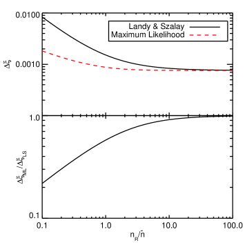
Figure 1.— Top panel: Standard deviation of the ML and LS estimators for $\xi$ as a function of the ratio of the random point density $n_{R}$ to the data point density $\bar{n}$. Bottom panel: The ratio of the standard deviations for the ML and LS estimators, $\Delta\xi_{ML}/\Delta\xi_{LS}$, as a function of $n_{R}/\bar{n}$. We have assumed a $(1~{}h^{-1}Gpc)^{3}$ survey with $\bar{n}=5\times 10^{-5}h^{3}\mbox{Mpc}^{-3}$, $R=100\ h^{3}\mbox{Mpc}$ and $\Delta R=10\ h^{-1}\mbox{Mpc}$. We have set $V_{1}=V_{2}=V_{shell}$.

Fig. 1 compares the standard deviations $\Delta\xi_{LS}$ and $\Delta\xi_{ML}$ of the LS and ML estimators as a function of $n_{R}/\bar{n}$, the ratio of the number density of random points to that of the data points. To make this plot, we hold the input parameter vector, $\mathbf{p}_{input}$, fixed, and vary the random point density as required. We have chosen parameters corresponding to a $(1\ h^{-1}\mbox{Gpc})^{3}$ survey with with $\bar{n}=5\times 10^{-5}\ h^{3}\mbox{Mpc}^{-3}$, $R=100\ h^{-1}\mbox{Mpc}$ and $\Delta R=10\ h^{-1}\mbox{Mpc}$. We have also imposed $V_{1}=V_{2}=V_{shell}$. We see that both the LS and ML estimators converge to the same value of $\Delta\xi$ at large $n_{R}$, but that the ML estimator converges much more quickly than the LS estimator.

We now explore how this relative performance depends on the various model parameters. Specifically, looking back at Eq. 35, the covariance matrix depends on four combinations of parameters: $\bar{n}V$, $n_{R}/\bar{n}$, $n_{R}V_{1}$, and $V_{1}/V_{2}$. We find that varying $\bar{n}V$ does not affect the relative performance of LS and ML, so we focus our attention on the remaining three parameter combinations. To further emphasize the difference between the ML and LS estimators, we now focus on the percent “excess error” in $\Delta\xi$ relative to the $n_{R}=\infty$ value of $\Delta\xi_{ML}$, i.e. we plot

$$\frac{\Delta\xi}{\Delta\xi_{ML}(n_{R}=\infty)}-1.$$ (81)

We remind the reader that in the Poisson limit that we are currently considering, both estimators yield the same $\Delta\xi(n_{R}=\infty)$.

Our results are shown in Fig. 2. The dashed and solid curves show the performance of the LS and ML estimators respectively, as a function of $n_{R}$, while holding $V_{1}$ fixed; i.e. the radial bin used to estimate $\xi$ is fixed. The three sets of curves correspond to three different values for $V_{1}$, or equivalently, three different radial bin-widths. Finally, the three panels explore different choices of $V_{1}/V_{2}$. Throughout, we have set $V_{2}=V_{shell}$, so that varying $V_{1}/V_{2}$ is equivalent to varying $V_{1}/V_{shell}$. We expect this should provide a worst-case scenario for the ML estimator, since the variance of $\xi$ increases with $V_{2}$.

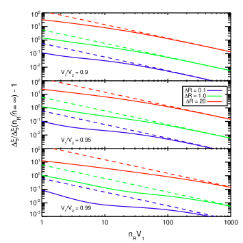
Figure 2.— The performance of the ML estimator relative to the LS estimator on uniform (Poisson) galaxy fields. Solid lines represent the performance of ML while dashed lines show the performance of LS. We have assume a $(1h^{-1}\mbox{Gpc})^{3}$ survey and $R=100h^{-1}\mbox{Mpc}$. We have fixed $V_{2}=V_{shell}$ (the most conservative assumption for the ML estimator) and show the effect of varying $n_{R}$, $\Delta R$ and $V_{1}/V_{2}$.

Fig. 2 confirms our observation that in the limit that $n_{R}$ becomes very large, the ML estimator approaches the LS estimator. It can also be seen in the figure that the ML estimator becomes significantly better than LS when $n_{R}V_{shell}\lesssim 100$, and that this requirement is relatively independent of the other parameters. Likewise, the improvement of the ML estimator relative to the LS estimator is stronger when $V_{1}/V_{2}\approx 1$.

There is an alternative way of viewing the improved performance of the ML estimator that is particularly well suited to a discussion of computational efficiency. Specifically, given an LS estimator with a random point density $(n_{R}/\bar{n})_{LS}$, one can determine the random point density $(n_{R}/\bar{n})_{ML}$ required for the ML estimator to achieve the same precision. Fig. 3 shows this ML random point density as a function of the LS random point density. Since typical pair counting algorithms on $N$ points scale as $O(N\sqrt{N})$, this reduction in the number of required random points means that the computation of $\xi$ can be made significantly faster. Because the overall improvement depends on $V_{2}/V_{1}$, we postpone a more quantitative discussion until after we estimate this ratio from numerical simulations below.

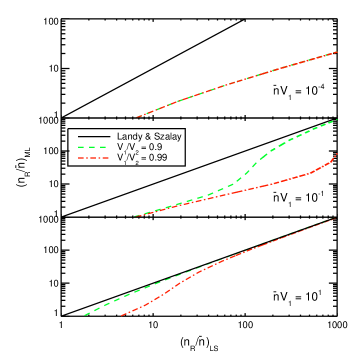
Figure 3.— The random point density $(n_{R}/\bar{n})_{ML}$ necessary for the ML estimator to match the precision of the LS estimator with a random point density $(n_{R}/\bar{n})_{LS}$.

As a final note before we turn our attention to numerical simulations, we also found the ML estimator for $\bar{n}$ outperforms the standard estimator

$$\hat{\bar{n}}=n_{R}\frac{D}{R}.$$ (82)

Specifically, if $D\lesssim 10^{4}$ and $(n_{R}/n_{D})\leq 10$, then the ML estimator can outperform the standard estimator by a significant margin. Modern galaxy surveys have $D\gg 10^{4}$ galaxies, so this result is only significant for estimating the density of rare objects, e.g. galaxy clusters. Note, however, that in that case, it is easy to ensure that $(n_{R}/\bar{n})$ is very large, so implementing the ML estimator is not necessary. Still, this result was interesting enough we thought it worth mentioning.

3.2. ML Performance: Numerical simulation

We have seen above that the ML estimator always performs at least as well as LS, and that in some regimes it performs significantly better. We now address two related questions:

• Are our Fisher matrix results representative of simulated data?

• Do we expect an actual survey to fall in a regime where the ML estimator significantly outperforms the LS estimator? In other words, what values of $V_{1}$ and $V_{2}$ are characteristic of an actual survey?

We address these questions through numerical simulations.

3.2.1 Numerical Simulations

For the $\xi=0$ case that we are considering at this point, generating a catalog of galaxy positions is trivial. We focus on two possible survey geometries:

1. Cube: a cube with side length $1h^{-1}\mbox{Gpc}$

2. Survey: a slab of dimensions $2.24~{}h^{-1}\mbox{Gpc}$ $\times$ $2.05~{}h^{-1}\mbox{Gpc}$ $\times$ $0.22~{}h^{-1}\mbox{Gpc}$ from which we have removed a $1\ h^{-1}\mbox{Mpc}$ $\times$ 2.05 $h^{-1}$Gpc$\times$ 0.22 $h^{-1}$Gpc  slice every 10 $h^{-1}$Mpc  along the longest dimension of the slab. In other words, this survey mask is composed of $\sim 200$ individual rectangular slabs separated by $1\ h^{-1}\mbox{Mpc}$ gaps.

The cube geometry is far simpler than the survey mask of any realistic survey, while the mask adopted in the survey configuration has far more boundary effects than any real survey is likely to have. Thus, the combination of the two should nicely bracket any real world scenario.

In practice, our catalog is generated in the cubical geometry and then remapped into the slab geometry using the technique of Carlson and White (2010). Although this remapping procedure is unnecessary here as the galaxies are not clustered, it will be important when we subsequently introduce clustering (and it explains the somewhat odd dimensions of our slab).

We perform pair counting on multiple realizations of the simulated catalogs using a kd-tree pair counting algorithm. For illustrative purposes, we consider two different scales:

1. Large: 100-101 $h^{-1}\mbox{Mpc}$

2. Small: 2-3 $h^{-1}\mbox{Mpc}$

These scales are chosen to encompass the wide range over which the correlation function is measured in actual data. At the largest scales, the correlation function is used as a probe of cosmology (e.g. by measuring the BAO feature) while at the smallest scales, the correlation function is used as a probe of galaxy formation and other physics.

3.2.2 Computing $V_{1}$ and $V_{2}$ on Simulated Catalogs

It is important to accurately estimate $V_{1}$ and $V_{2}$ because, as shown above, the effectiveness of the ML estimator depends on their values. As $V_{2}$ only enters the covariance matrix (and not the mean) of observables, estimating it accurately requires computing the observables over many realizations of survey volume. By contrast, $V_{1}$ can be estimated easily by averaging over these realizations: $\hat{V_{1}}=2\left<RR\right>/\left(\bar{n}^{2}V\right)$, where the angled brackets indicate an average over the different realizations. We estimate $V_{2}$ by maximizing a likelihood

$$\mathcal{L}\left(V_{2}|\{\mathbf{x}\}\right) \propto \prod_{i}^{N_{realizations}}\frac{1}{\sqrt{\det\mathbf{C}(V_{2})}}$$

$$\times \exp \left(-\frac{1}{2}\left(\mathbf{x}_{i}-\left\langle\mathbf{x}\right\rangle\right)^{T}\cdot\mathbf{C}^{-1}\left(V_{2}\right)\cdot\left(\mathbf{x}_{i}-\left\langle\mathbf{x}\right\rangle\right)\right),$$ (83)

where the other parameters have been fixed. When maximizing the likelihood, we enforce the physical requirement that $V_{1}<V_{2}$.

We have have used 700 realizations of the survey volume when computing the best fit values of $V_{1}$ and $V_{2}$. The results are summarized in Table 1. The first four rows of that table show the values of $V_{1}/V_{shell}$ and $V_{2}/V_{shell}$ computed directly from the simulations, while the final two rows show the value of $V_{1}/V_{2}$. For the small scale case, the constraint on $V_{2}/V_{shell}$ is very noisy owing to the low number of galaxies within the small scale shells. The noise is large enough that our best fit value of $V_{2}/V_{shell}$ violates the inequality in Eq. 52 (although it is consistent at $\sim 1.4\sigma$). Rather than use this noisy value of $V_{s}/V_{shell}$ in the results that follow, we have set $V_{2}=V_{shell}$ to get the most conservative (lower) limit on $V_{1}/V_{2}$. For the large scale case, the noise is much less and we are able to use the value of $V_{2}$ computed from the simulations. As we have seen above, lowering the value of $V_{1}/V_{2}$ worsens the performance of the ML estimator. From Table 1 it is clear that $V_{1}/V_{2}>0.95$ is a conservative lower limit that should apply even in fairly wild survey geometries.

As discussed above, the important control parameters for the ML estimator are $\bar{n}V_{1}$ and $V_{1}/V_{2}$. For a survey with a typical number density of $\bar{n}=5\times 10^{-5}h^{3}\mbox{Mpc}^{-3}$, our $V_{1}$ results correspond to $\bar{n}V_{1}$ values of roughly 0.004 and 30 for the small and large scales respectively (ignoring the relatively small differences in $\bar{n}V_{1}$ for the two survey geometries). The value of $V_{2}/V_{1}$ is slightly more difficult to ascertain. At the large scale, we find that $V_{1}/V_{2}\gtrsim 0.95$ for the three survey geometries considered. At small scales, our measurement of $V_{2}$ is too noisy to get a good estimate of $V_{1}/V_{2}$. However, we have demonstrated that $V_{1}<V_{2}<V_{shell}$ so $V_{1}/V_{2}\geq V_{1}/V_{shell}=0.986$. Looking back at Fig. 2, we expect the ML estimator to significantly outperform the LS estimator at small scales. At large scales, the value of $\bar{n}V_{1}$ is large enough that we expect the improvement of LS over ML to be more modest (although still significant for $n_{R}/\bar{n}\lesssim 100$). Of course, if the width of the large scale shell is reduced so that $n_{R}V_{1}$ goes down, we expect ML to begin to significantly outperform LS.

Table 1Fits to $V_{1}$ and $V_{2}$ computed on numerical simulations.

	Cube	Survey
$V_{1}/V_{shell}$ small scale	$0.9965\pm 0.0008$	$0.9862\pm 0.0007$
$V_{1}/V_{shell}$ large scale	$0.8531\pm 0.0006$	$0.6579\pm 0.0003$
$V_{2}/V_{shell}$ small scale	$1.9\pm 0.9$	$2.3\pm 0.9$
$V_{2}/V_{shell}$ large scale	$0.886\pm 0.008$	$0.689\pm 0.005$
$V_{1}/V_{2}$ small scale	$\geq 0.9965\pm 0.0008$	$\geq 0.9862\pm 0.0007$
$V_{1}/V_{2}$ large scale	$0.963\pm 0.009$	$0.955\pm 0.008$

3.2.3 Computing the Maximum Likelihood Estimator on a Simulated Data Catalog

The likelihood in Eq. 76 depends on the model parameters through both the expectation values of the observables, $\left<\mathbf{x}\right>$ and the covariance matrix $\mathbf{C}$. However, we have found that we can obtain very accurate results by simply evaluating the covariance matrix for parameters that are reasonably close to $\hat{\mathbf{p}}_{ML}$, and – keeping the covariance matrix fixed – vary the parameters in $\left<\mathbf{x}\right>$ to maximize the likelihood. Our approach simplifies the calculation of $\hat{\mathbf{p}}_{ML}$ significantly so that it reduces to several inversions of a $5\times 5$ matrix. This means that calculating $\hat{\xi}_{ML}$ is not significantly more difficult computationally than calculating $\hat{\xi}_{LS}$.

We note we have explicitly verified that in the Poisson case, the derivatives of $\mathbf{C}$ can be safely neglected. For clustered fields, this is difficult to show in general, but one can make a rough argument. As an illustrative example, consider the $2pt$ contribution. In the limit of a large survey, we can rewrite Eq. 43 as a sum over radial bins $R^{\prime}$ with $R^{\prime}\leq R_{survey}$, so that

$$V^{2}2pt=V\sum V_{shell}(R^{\prime})\xi(R^{\prime}).$$ (84)

Taking the derivative of $2pt$ with respect to $\xi(R)$ we find

$$\frac{d2pt}{d\xi(R)}=\frac{V_{shell}(R)}{V}\ll 1,$$ (85)

so that, relative to the mean, the information on $\xi(R)$ from the sample variance covariance matrix is always being multiplied by factors of $V_{shell}(R)/V$. Perhaps from a more physical perspective, this can also be argued by noting that the sample variance integrals are dominated by survey-volume scale modes, with small scale modes contributing little because of the filtering by the survey window function.

Computing the maximum likelihood estimator in the fashion described above requires making a choice for the covariance matrix used to analyze the data. We will consider two possibilities for this covariance matrix: (1) the true covariance matrix from which the data is generated, and (2) forming an estimate of the covariance matrix from the data itself (setting $V_{2}=V_{shell}$). The first possibility represents the best we could hope to do: we are analyzing the data using the same covariance matrix that was used to generate it.

In the second case, we form an estimate of the covariance matrix from the observed data (i.e. a new covariance matrix for each set of observables) and then compute the maximum likelihood estimator using this covariance matrix estimate. To form the estimate of the covariance matrix, we re-express the Poisson covariance matrix in terms of clustering observables. For instance, since $\left\langle D\right\rangle=\bar{n}V$, and $\mbox{Var}(D)=\bar{n}V$, we simply set $\mbox{Var}(D)=D$ in the covariance matrix. Similarly, setting $R$, and $RR$ to their expectation values (see §2.2), we can solve for the various terms that appear in the covariance matrix as a function of the clustering observables $D$, $R$, and $RR$. The exception to this rule is $V_{2}$, for which we simply assume $V_{2}=V_{shell}$. The full covariance matrix obtained in this way is

$$\mathbf{C}=\left(\begin{array}[]{ccccc}D&0&\rho RR&2\rho^{2}RR&0\\ \mbox{---}&R&\rho RR&0&2RR\\ \mbox{---}&\mbox{---}&\frac{1}{2}\rho RR\left[N_{s}\left(1+\rho\right)+1\right]&\rho^{2}N_{s}RR&\rho N_{s}RR\\ \mbox{---}&\mbox{---}&\mbox{---}&2\rho^{2}RR\left[\rho N_{s}+\frac{1}{2}\right]&0\\ \mbox{---}&\mbox{---}&\mbox{---}&\mbox{---}&2RR\left[N_{s}+\frac{1}{2}\right]\end{array}\right),$$ (86)

where we have defined $\rho=D/R$ and $N_{s}=n_{R}V_{shell}$. Note that since $n_{R}$ is known (it is chosen by the observer), the above expression can be computed with no a priori knowledge of the input model parameters $\mathbf{p}_{input}$.

Given one of the above choices for the covariance matrix, we now wish to maximize the likelihood while keeping the covariance matrix fixed. For numerical purposes, it is convenient to reparameterize the parameter space using a new vector $\mathbf{p}^{\prime}=\{\bar{n},V,\alpha,\beta\}=\{\bar{n},V,VV_{1},VV_{1}(1+\xi)\}$ such that the expectation value of the observed data vector, $\left\langle\mathbf{x}\right\rangle$, is linear in $V$, $\alpha$ and $\beta$. With this reparameterization, maximizing $\mathcal{L}$ given $\bar{n}$ reduces to a simple matrix inversion problem, so the overall minimum can be easily found using standard 1-dimensional minimization routines.

3.2.4 Comparing the Numerical and Analytic Calculations of the ML Estimator

Ideally, to test the two estimators we would generate many simulated data catalogs, perform pair counting on each one, and compute the corresponding ML and LS estimators. However, pair counting on many catalogs for very high $n_{R}$ is prohibitively expensive from a computational point of view. Instead, we make a small number of realizations of the survey at reasonable $n_{R}$ and use these realizations to compute the unknown terms in the covariance matrix – $V_{1}$ and $V_{2}$ – as described above. We then generate $10^{5}$ Monte Carlo realizations of our clustering observables $\mathbf{x}=\{D,R,DR,DD,RR\}$ by drawing from a multivariate Gaussian with the calibrated covariance matrix. Using our Monte Carlo realizations, we compute the mean and standard deviation of each of our estimators in order to test whether the estimators are unbiased, and the relative precision of the two estimators.

Fig. 4 compares the result of our numerical experiment to the analytic results presented in the last section. The red and black shaded regions represent the results of our numerical experiment for the ML and LS estimators respectively; the width of these regions represents the error on $\Delta\xi$ owing to the finite number of realizations. The solid red and black lines represent the theoretical behavior predicted from the Fisher matrix as described above. We see that the results of our numerical experiment are in good agreement with the results of the Fisher calculation. For this plot we assumed the cubical geometry discussed above; the upper panel corresponds to the small scale, while the lower panel corresponds to the large scale.

The blue line in Fig. 4 shows the ML curve when the covariance matrix is estimated directly from the data using the technique described above. As can be seen, this simple method for estimating the covariance matrix produces results that are as good as the case when the true covariance matrix is exactly known. Thus, we can firmly conclude that in the regimes described above – namely low $n_{R}V_{1}$ and $V_{1}/V_{2}\sim 1$ – the ML estimator represents a significantly more powerful tool for estimating the correlation function than the LS estimator.

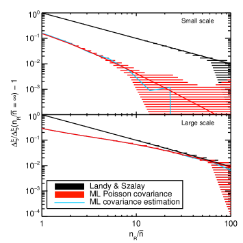
Figure 4.— Comparison of ML and LS estimators for $\xi$ calculated using simulated galaxy data in the Poisson limit. $\Delta\xi$ is the standard deviation over many random realizations of the observables of the estimator for $\xi$. The curves have been normalized to the value of the estimator for very large $n_{R}/\bar{n}$. The shaded regions represent the errors on the measured quantities owing to the finite number of simulations. The solid cuves represent the behavior predicted from the analytic calculations described above. The blue curve corresponds to the ML estimator obtained when expressing the covariance matrix in terms of the clustering observables, as opposed to fixing the covariance matrix to its true value (and setting $V_{2}=V_{1}$). The survey parameters have been chosen to match the cubical survey geometry; upper panel is for the small scale, while the lower panel is for the large scale.

4. ML Performance: Clustered Fields

Clustering of galaxies introduces new terms into the covariance matrix of the observables $\mathbf{x}=\{D,R,DR,DD,RR\}$. These new terms involve various integrals of the correlation function and its higher moments over the survey volume (see Eq. 41). Consequently, we no longer expect the LS estimator to be the large volume, large $n_{R}$ limit of the ML estimator.

Our program here will be very similar to that discussed above for the case with no clustering. The major difference is that in the present case, the covariance matrix of the observables is more difficult to calculate as it depends on the detailed clustering properties of the galaxies. One consequence of this fact is that we cannot easily include the dependence of the covariance matrix on $\xi$ in the Fisher matrix calculation as we did previously. Instead, we will consider the covariance matrix to be fixed. This means that we are throwing out some information, but as we have seen above, including the dependence of the covariance matrix on the model parameters does not significantly affect our constraints on $\xi$.

4.1. ML Performance: Analytic Estimates

As we did previously, we can estimate the errors on our ML estimate of $\xi$ using the Fisher matrix. We set $C_{,i}=0$ in Eq. 77 as the dependence of $C$ on $\xi$ is not known. To estimate $C$ requires computing the $2pt$, $2pt_{b}$, $3pt$, and $4pt$ terms. For our Fisher analysis, we choose to perform the calculation of these terms analytically assuming the Gaussian, large volume, spherical survey limit discussed above. This allows us to express the clustering terms as one-dimensional integrals over the power spectrum (i.e. Eqs. 55, 56, 57, 58, and 59). Therefore, given a power spectrum, we can compute the full covariance of the observables, which in turn allows us to compute the Fisher matrix, and therefore, the error on $\xi$. We use the power spectrum output from CAMB (Lewis et al., 2000) assuming standard $\Lambda$CDM cosmological parameters that are consistent with the results of WMAP9 (Bennett et al., 2012): $h=0.7$, $\Omega_{c}h^{2}=0.1127$, $\Omega_{b}h^{2}=0.02254$, $n_{S}=1.0$. To convert the matter power spectrum into a galaxy power spectrum we have assumed a constant bias of $b=2$, appropriate for galaxies in a BOSS-like sample.

Fig. 5 shows the results of the Fisher analysis including the effects of galaxy clustering. This figure is analogous to the earlier Fig. 2 which applied to unclustered fields. Comparing the two figures reveals that clustering enhances the performance of ML relative to LS somewhat but that otherwise the qualitative behavior is very similar. The results from our discussion of the ML estimator on unclustered fields therefore carry over to clustered fields mostly unchanged.

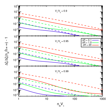
Figure 5.— The performance of the ML estimator relative to the LS estimator on clustered galaxy fields (analogous to Fig. 2 for unclustered fields). See text for details of our assumptions about cosmology and bias. Solid lines represent the performance of ML while dashed lines show the performance of LS. The errors on ML have been computed using the Fisher matrix, assuming a spherical survey with a volume of 1000 $h^{3}\mbox{Mpc}^{3}$, $\bar{n}=5\times 10^{-5}h^{3}\mbox{Mpc}^{-3}$, and $R=100h^{-1}\mbox{Mpc}$. We have set $V_{1}=0.97V_{shell}$, a resonable value for an actual survey (as illustrated above). We have set $V_{2}=V_{shell}$, which gives us the most conservative limit on the performance of the ML estimator.

4.2. ML Performance: Numerical Simulation

As we have done for the unclustered fields, we would now like to connect the results of our Fisher matrix study to results obtained from analyzing simulated realizations of the pair counts observables for clustered galaxy fields. There are two reasons for going beyond the Fisher marix estimates. First, the simulated realizations allows us to measure $\mathbf{C}_{\rm{clustering}}$ in a survey that is more realistic than a sphere; as we will see, this change in geometry significantly impacts the values of the clustering terms. Second, having simulated data allows us to experiment with analyzing this data using different covariance matrices. This is important, as estimating the true observable covariance matrix for clustered galaxy fields is non-trivial.

Measuring the clustering contribution to the covariance matrix requires realizations of a clustered galaxy field. While it is conceivable that the observable covariance matrix could be estimated from a single cosmological realization using a jackknife, we have found that this approach does not yield reliable results at large scales. In the jackknife approach, chunks of the survey volume — which must be significantly larger than the scales of interest — are removed and the pair observables are recalculated; the covariance matrix of the observables can then be related to the covariance across the jackknives. We suspect that the reason this approach does not work in practice is that when dealing with large scales, the size of the removed chunks becomes significant enough that they effectively change the values of $V$, $V_{1}$, and $V_{2}$ relative to what they were before each chunk was removed. Consequently, the pair observables computed on the jackknifed survey volume are not drawn from the same underlying covariance matrix as the observables in the full survey volume.

Rather than attempt to address the problems with the jackknives, we instead estimate the observable covariance matrix from multiple realizations of an N-body simulation. We use 41 cosmological realizations of a $(2400\,h^{-1}\mbox{Mpc})^{3}$ volume produced by the LasDamas group (McBride et al., 2011). The LasDamas simulations assume a flat $\Lambda$CDM cosmology described by $\Omega_{m}=0.25$, $\Omega_{\Lambda}=0.75$, $\Omega_{b}=0.04$, $h=0.7$, $\sigma_{8}=0.8$ and $n_{s}=1$. For our “galaxies”, we rely on the halo catalog, randomly selecting halos (restricting to $M\geq 10^{13}\,h^{-1}M_{\odot}$) to achieve the desired number density. Henceforth, we will consider the measurement of the correlation function in a radial bin extending from $R=50\,h^{-1}\mbox{Mpc}$ to $R=60\,h^{-1}\mbox{Mpc}$. This radial bin was chosen as it is small enough to be significantly impacted by clustering and big enough to contain a large number of galaxies so that the impact of counting noise is minimized.

We estimate the $2pt$, $2pt_{b}$, $3pt$, and $4pt$ terms in a manner similar to that used to estimate $V_{2}$ above. First, we estimate $\bar{n}$, $n_{R}$, $V$ and $V_{1}$ using the expressions we have derived for the expectation values of the pair counts observables. $V_{2}$ is then estimated by maximizing a likelihood as in Eq. 3.2.2. Since the $D$, $DR$ and $DD$ observables are now affected by clustering, however, we consider only the $R$ and $RR$ observables when evaluating the likelihood in Eq. 3.2.2. With estimates of $\bar{n}$, $n_{R}$, $V$, $V_{1}$ and $V_{2}$ in hand, we can form an estimate of $\mathbf{C}_{\rm{Poisson}}$. Finally, to determine the clustering terms, we maximize the four dimensional likelihood function defined by

$$\mathcal{L}\left(\{2pt,2pt_{b},3pt,4pt\}|\{\mathbf{x}\}\right)\propto$$

$$\prod_{i=1}^{N_{realizations}}\frac{1}{\sqrt{\det\mathbf{C}}}\times\exp\left(-\frac{1}{2}\left(\mathbf{x}_{i}-\left\langle\mathbf{x}\right\rangle\right)^{T}\cdot\mathbf{C}^{-1}\cdot\left(\mathbf{x}_{i}-\left\langle\mathbf{x}\right\rangle\right)\right)$$ (87)

where

$$\mathbf{C}=\mathbf{C}_{Poisson}+\mathbf{C}_{clustering}(2pt,2pt_{b},3pt,4pt),$$ (88)

and, in our case, $N_{realizations}=41$. The results of this fitting procedure are shown in Fig. 6. It is clear from the figure that we obtain no significant detection of the $2pt$ and $3pt$ terms. The fact that there is no signficant $3pt$ detection is not surprising as the galaxy field is roughly Gaussian. The non-detection of the $2pt$ term, on the other hand, can be attributed to the fact that we only have $41$ realizations of the survey volume and therefore our $2pt$ estimate is noisy. The numerical results for our fits are shown in Table 2.

Although we apparently do not have the constraining power to robustly estimate the $2pt$ term from the N-body simulations, we can estimate it analytically using Eq. 53. For the cubical geometry that we consider here, we can integrate Eq. 53 exactly to obtain an estimate for $2pt$. Performing this calculation requires an estimate of the power spectrum, $P(k)$, which we obtain from CAMB (Lewis et al., 2000). The bias is determined by matching the prediction for $\xi$ from the power spectrum to its measured value at the scale of interest; we find that the bias is roughly $b=1.6$. Our analytic estimate of $2pt$ is shown as a red line in Fig. 6; the numerical value of $2pt=2.2\times 10^{-7}$ is in good agreement with the result from the N-body simulations shown in Table 2.

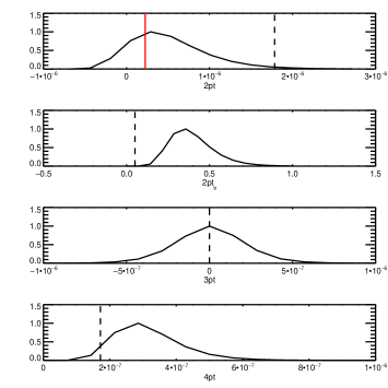
Figure 6.— The results of our fit for the clustering terms in the covariance matrix to data from N-body simulations. The curve in each panel represents the probability distribution from the fit for the corresponding parameter. The solid vertical line (red in the online version) in the top panel represents our prediction for $2pt$ from integrating Eq. 53 assuming the true cubical geometry of the simulation. Dashed vertical lines in all panels represent predictions for the n-point terms obtained by integrating the expressions we have derived for them assuming the large volume, spherical survey limit (see §2.3).

Table 2Fits to clustering terms computed from N-body simulations.

	$R=50h^{-1}\mbox{Mpc}$, $\Delta R=10h^{-1}\mbox{Mpc}$
$2pt$	$(4\pm 4)\times 10^{-7}$
$2pt_{b}$	$0.4\pm 0.1$
$3pt$	$(0\pm 6)\times 10^{-8}$
$4pt$	$(3\pm 1)\times 10^{-7}$

With our estimates of the $2pt_{b}$, $3pt$, and $4pt$ terms from the fits to the cosmological realizations, and our estimate of $2pt$ by direct integration, we can now compute the full covariance matrix of observables. We use this covariance matrix to generate realizations of the observables as we have done above for the case without galaxy clustering. The results of our analysis of these simulated data sets are presented in Fig. 7. As in Fig. 4, the black curve represents the analytic prediction for the errors obtained using the LS estimator and the shaded region represents the measurement of the errors on simulated data (the width of the region shows the error on this measurement owing to a finite number of realizations). The red curve represents the prediction from the Fisher matrix for the ML estimator, while the red shaded region represents the numerical results computed by analyzing the data using the covariance matrix that was used to generate it.

The analyst wishing to compute the correlation function in a galaxy survey with the ML estimator must first estimate the covariance matrix of $D$, $DR$, $DD$, and $RR$. In the unclustered case considered previously, the estimation process was straightforward: we simply computed $\bar{n}$, $V$, and $V_{1}$ from the observables $D$, $R$, and $RR$, and we set $V_{2}=V_{1}$, and then substituted into Eq. 35. We showed (blue curve in Fig. 4) that this procedure works well. In the present case, however, computing the observable covariance matrix is more difficult as it depends on the $2pt$, $3pt$, $4pt$, and $2pt_{b}$ terms, which are not known a priori, and are difficult to estimate from the data.

There are several ways around this difficulty. The simplest is to ignore the clustering contribution to the covariance matrix and simply compute the covariance matrix in the Poisson limit as above (using only the $R$ and $RR$ observables as these are unaffected by galaxy clustering) for the purposes of defining the ML estimator. Figure 7 compares the performance of this simple approach (blue curve) to the LS estimator and to the ML estimator when run using the correct covariance matrix. It appears that the Poisson covariance matrix approach generally does better than LS but that it does not achieve the maximal performance that can be obtained with the ML estimator using the true covariance matrix. We note that we have also checked that using the Poisson covariance matrix did not bias the resulting ML estimator.

Alternatively, one can use our analytic estimates of the covariance matrix of clustered fields to analyze the data. There are several ways that one could go about this in deail; we take an approach that requires little computational work. As the $2pt$ function can be easily estimated by integrating Eq. 53 for a cubical geometry, we estimate $2pt$ in that way. The remaining clustering terms ($2pt_{b}$, $3pt$, and $4pt$) are more difficult to estimate in a cubical geomtry, but can easily be estimated for a spherical geometry using Eqs. 56 and 57 (we assume that the distribution is Guassian so that the $3pt$ term vanishes). As seen in Fig. 6, these estimates of the clustering terms are not perfect, but they at least give us some handle on the magnitude of the clustering contribution. Our easy-to-compute estimate of the clustering contribution to the covariance matrix can then be combined with an estimate of the Poisson contribution (as above) to form an estimate of the total covariance matrix. The green curve in Fig. 7 shows the results of analyzing the data using this covariance matrix. We see that this approach generally does better than using only the Poisson covariance matrix, but that it does not do quite as well as using the true covariance matrix.

Finally, one could derive accurate estimates by running several numerical simulations and computing the covariance of the observables across these simulations. Such simulations are typically already perfomed in order to estimate statistical uncertainties, and so this step should not require any additional overhead. This approach can be simulated by using some small number, $N_{realization}$, of the realizations to compute an observable covariance matrix, and then analyzing the data using this covariance matrix. We test this method by using our input covariance matrix to generate $N_{realizations}=40$ independent data realizations, which in turn are used to estimate the covariance matrix of the generated data. This estimated covariance matrix is then used to estimate $\xi$. The purple curve in a new independent data set. Fig. 7 shows the errors on $\xi$ calculated in this way. We see that 40 realizations is sufficient to capture the clustering information in the covariance matrix for the purposes of the ML estimator.

One might worry about the circularity of estimating the covariance matrix in the manner described above; after all, the clustering terms in Eq. 41 depend precisely on the correlation function that we are trying to measure. However, as we have seen above, incorrectly estimating the covariance matrix does not lead to a bias in the recovered $\hat{\xi}_{ML}$, but rather increases its variance. Furthermore, even if the clustering terms are set to zero, we still get a lower variance estimate of $\xi$ than with LS. Any reasonable errors in the cosmology used to estimate the covariance matrix will never cause the ML estimator to perform worse than LS. Finally, if an analyst is really worried about obtaining the absolutely minimum variance estimator of $\xi$, it is always possible to apply the ML estimator in an iterative fashion. One simply assumes a cosmology when calculating the observable covariance matrix, and then adjusts the cosmology based on the recovered $\hat{\xi}_{ML}$; the process can then be repeated until convergence is reached.

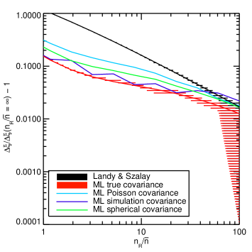
Figure 7.— The performance of the ML estimator relative to the LS estimator on clustered galaxy fields (analogous to Fig. 4 for unclustered fields). Black and red lines represent analytic predictions for the LS (using Eq. 79) and ML estimator (using the Fisher matrix) respectively. Black and red shaded regions represent the error bands corresponding to these two estimators computed from numerical simulations. The remaining curves represent the results obtained when the simulated data is analyzed with the ML estimator using different choices of the covariance matrix. Blue corresponds to using a Poisson covariance matrix estimated from the data; purple corresponds to using the mean covariance matrix computed from $40$ realizations of the survey volume; green corresponds to computing the clustering contribution covariance matrix analytically as described in the text (using the spherical approximation for the $2pt_{b}$ and $4pt$ terms).

5. Discussion

We have explored the utility of the ML estimator for computing galaxy correlation functions. The ML estimator makes use of the same pair-counting observables as the standard LS estimator, yet the former significantly outperforms the latter in certain regimes. Moreover, because all but one of the parameters in the likelihood model are linear (assuming we use a fixed covariance matrix, as described above), the likelihood maximization is numerically trivial. Consequently, we see no reason not to switch from LS estimators to ML estimators: the ML estimator is always better, and has no significant computational requirements in excess of those for the LS estimator. In short, there are only upsides to using the ML estimators, and no real downsides.

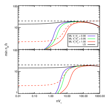
Figure 8.— The minimum value of $n_{R}$ required to achieve convergence at the 5% level to the value of $\Delta\xi$ at $n_{R}=\infty$ , as a function of $\bar{n}V_{1}$. We have assumed a spherical survey with volume $V=(2400h^{-1}\mbox{Mpc})^{3}$. The two panels correspond to different radial scales: upper panel is for $R=50h^{-1}\mbox{Mpc}$ to $60h^{-2}\mbox{Mpc}$ while lower panel is for $R=100h^{-1}\mbox{Mpc}$ to $101h^{-2}\mbox{Mpc}$. Dashed lines (which do not depend on the radial scale) represent the case where there is no clustering.

For an analyst wishing to compute the correlation function from a galaxy survey, an important question is how large must the random catalog be in order to get errors on $\xi$ that are close to what would be obtained with an infinite random catalog? In Fig. 8 we plot the minimum value of $n_{R}/\bar{n}$ required to obtain errors on $\xi$ that are within 5% of the value of $\Delta\xi$ at $n_{R}=\infty$ for both the ML and LS estimators. As we have discussed previously, the ML estimator allows one to compute the correlation function to the same precision as with LS while using a significantly smaller random catalog. We see that LS acheives convergence to the 5% level at $n_{R}/\bar{n}\sim 15$. Depending on the value of $\bar{n}V_{1}$, the ML estimator can reduce the required value of $n_{R}$ by up to a factor of 7.

Perhaps the single biggest obstacle one faces from the point of view of implementing the ML estimator is that one must specify the covariance matrix used to minimize $\chi^{2}$. In practice, however, we do not believe this is a particularly problematic issue. Firstly, modern cosmological analysis typically rely on extensive numerical simulations to calculate the covariance matrix of survey observables. Just as one can use these numerical simulations to calibrate the variance in $\hat{\xi}_{LS}$, one can use the same simulations to estimate the covariance matrix of the observables $D$, $R$, $DR$, $DD$, and $RR$. With this covariance matrix at hand, one can then compute $\hat{\xi}_{ML}$, and use these same simulations to estimate the error $\Delta\hat{\xi}_{ML}$. Alternatively, because the simulation-based covariance matrices are expected to be correct, one could, if desired, treat the problem using Bayesian statistics as usual, without fear of underestimating uncertainties.

Our work can be compared to a recent paper by Vargas-Magaña et al. (2013) (hereafter VM). In that work, the authors construct an estimator that significantly outperforms LS on realistic surveys. In brief, their estimator is a linear combination of all possible ratios of the standard pair counts observables $\mathbf{x}=\{DD,DR,RR\}$ up to second order (see their Table 1), i.e.

$$\hat{\xi}=c_{0}+\sum_{i=1}^{6}c_{i}R_{i}+\sum_{y}^{18}c_{i}R_{i}^{(2)},$$ (89)

where $R_{i}$ are various ratios of elements of $\mathbf{x}$. The set of coefficients is calibrated using lognormal simulations of the survey with a known correlation function, with the coefficients dependent on the simulations and the survey geometry.

At first sight, an obvious objection to this approach is that because the optimal coefficients depend on the correlation function of the field, the sensitivity of the resulting estimator to choice of correlation function in the log-normal simulations makes this method undesirable. However, VM demonstrated that this problem can be solved with an iterative technique: one uses LS to estimate $\xi$, and then uses that $\xi$ to generate log-normal realizations, so that the data itself informs the simulations. These realizations are used to define the coefficients, which are then employed in the data to get a new estimate of $\xi$, and the whole procedure is iterated until convergence is achieved.

When we run our analysis mirroring the random point densities and binning scheme of VM, we find that the improvements of the ML estimator relative to the LS estimator are on the order of several percent, significantly lower than the improvements advertised by VM. Note, however, that Figure 7 demonstrates that the ML estimator saturates the Cramer–Rao bound on the variance of $\hat{\xi}$. As the estimator of VM uses the same pair counts observables as the ML estimator, the fact that the former violates the Cramer–Rao bound may at first appear problematic. The resolution to this problem is that for an arbitrary correlation function, the procedure of VM is biased and therefore the Cramer–Rao bound does not apply. The VM estimator is only unbiased for correlation functions whose shape can be fit by the particular form assumed in their iterative fitting procedure (Eq. 3 of their paper).

As a summary, we would say that if one wishes to quickly and easily estimate an arbitrary correlation function, we can unambiguously advocate the use of the ML estimator over the LS estimator. Under some circumstances, however, where the correlation function is known to be well fit by the form assumed by VM, their iterative scheme leads to a dramatic reduction of errors, at the expense of increased computational requirements and complexity.

5.1. Recipe for Computing the Maximum Likelihood Correlation Function Estimator

To aid the reader, we now provide a step-by-step guide of the steps required to implement our ML estimator.

1. Compute the observables $[D,R,DR,DD,RR]$ in the usual fashion.

2. Estimate the covariance matrix of observables:

   • In most cases, we expect this to be done via numerical simulations.

   • One may use a Poisson covariance matrix to analyze the data as in Eq. 86.

   • If desired/necessary, add analytic estimates of the clustering terms to the covariance matrix.

3. Maximize the likelihood defined in Eq. 76 to find $\hat{\xi}_{ML}$, keeping the covariance matrix fixed to the estimate from above. To do so, use the parameter vector $\mathbf{p}^{\prime}=\{\bar{n},V,\alpha,\beta\}=\{\bar{n},V,VV_{1},VV_{1}(1+\xi)\}$, and minimize $\chi^{2}$. With this redefinition, the only non-linear parameter in our expressions for the expectation values of the observables (Eqs. 14, 18, 21, 22, 23) is $\bar{n}$. Consequently, minimization can easily be achieved be defining a grid in $\bar{n}$. For each grid point, one finds the maximum likelihood value for the linear parameters through straightforward matrix inversion, and then evaluates the likelihood. The overall minimum can easily be estimated from the data grid.

Before we end, there in one last additional point that is worth noting with regards to correlation function estimators. In particular, our formalism and maximum likelihood framework also suggests what are ideal binning conditions. Specifically, in order to gaurantee that the Gaussian likelihood approximation is good, one should adopt radial bins such that $DD\gg 1$. If one sets $DD=100$, the corresponding bin width $\Delta\ln R=\Delta R/R$ for a scale R should be

$$\Delta\ln R=1.59\left(\frac{1\ \mbox{Mpc}}{R}\right)^{3}\left(\frac{1\ \mbox{Gpc}^{3}}{V}\right)\left(\frac{10^{-4}\ \mbox{Mpc}^{-3}}{\bar{n}}\right)^{2}.$$ (90)

At BAO scales, this suggests that the minimal radial width which one can bin data is therefore $\Delta\ln R\approx 10^{-6}$. This corresponds to exceedingly small angular bins, where the ML estimator is expected to be much superior to the LS estimator. In practice, binning as fine as this is unnecessary, but it does highlight that the ML estimator should enable finer binning than the LS estimator.

Appendix A Derivation of $\mbox{Var}(DD)$

We present here a derivation of our expression for $\mbox{Var}(DD)$ in Eqs. 35 and 41. The remaining terms in the covariance matrix can be derived in a similar fashion. We have by definition

$$\mbox{Var}(DD)=\left<\left(DD(r)\right)^{2}\right>-\left<DD(r)\right>^{2}.$$ (A1)

It was shown in the text that

$$\left<DD(r)\right>=\frac{1}{2}\bar{n}^{2}VV_{1}\left[1+\xi(r)\right].$$ (A2)

Considering the remaining term in $\mbox{Var}(DD)$ and using Eqs. 10 and 12, we find

$$\left<(DD(r))^{2}\right> = \frac{1}{4}\left<\sum_{ijkl}\Delta V^{4}\bar{n}^{4}(1+\delta_{i})(1+\delta_{j})(1+\delta_{k})(1+\delta_{l})W_{ij}W_{kl}S_{i}S_{j}S_{k}S_{l}\right>$$ (A7)

$$= \frac{1}{4}\left<\sum_{ijkl}\Delta V^{4}\bar{n}^{4}(1+\delta_{i}\delta_{j}+\delta_{i}\delta_{k}+\delta_{i}\delta_{l}+\delta_{j}\delta_{k}+\delta_{j}\delta_{l}+\delta_{k}\delta_{l}+\right.$$

$$\left.\delta_{i}\delta_{j}\delta_{k}+\delta_{i}\delta_{j}\delta_{l}+\delta_{i}\delta_{k}\delta_{l}+\delta_{j}\delta_{k}\delta_{l}+\delta_{i}\delta_{j}\delta_{k}\delta_{l})W_{ij}W_{kl}S_{i}S_{j}S_{k}S_{l}\vphantom{\sum_{ijkl}}\right>$$

$$= \frac{1}{4}\sum_{ijkl}\Delta V^{4}\bar{n}^{4}\left[1+\frac{\delta_{ik}}{\bar{n}\Delta V}+\frac{\delta_{il}}{\bar{n}\Delta V}+\frac{\delta_{jk}}{\bar{n}\Delta V}+\frac{\delta_{jl}}{\bar{n}\Delta V}+\right.\xi_{ij}+\xi_{ik}+\xi_{il}+\xi_{jk}+\xi_{jl}+\xi_{kl}$$

$$\left.+\left<\delta_{i}\delta_{j}\delta_{k}+\delta_{i}\delta_{j}\delta_{l}+\delta_{i}\delta_{k}\delta_{l}+\delta_{j}\delta_{k}\delta_{l}+\delta_{i}\delta_{j}\delta_{k}\delta_{l}\right>\vphantom{\frac{\delta_{jl}}{\bar{n}\Delta V}}\right]W_{ij}W_{kl}S_{i}S_{j}S_{k}S_{l}\vphantom{\sum_{ijkl}}$$

$$= \frac{1}{4}\sum_{ijkl}\Delta V^{4}\bar{n}^{4}W_{ij}W_{kl}S_{i}S_{j}S_{k}S_{l}+\sum_{ij}\Delta V^{3}\bar{n}^{3}W_{ij}W_{ik}S_{i}S_{j}S_{k}+\frac{1}{2}\sum_{ij}\Delta V^{4}\bar{n}^{4}\xi(r)W_{ij}W_{kl}S_{i}S_{j}S_{k}S_{l}+\bar{n}^{4}\sum_{ijkl}\Delta V^{4}\xi_{ik}W_{ij}W_{kl}S_{i}S_{j}S_{k}S_{l}$$

$$+\bar{n}^{4}\left<\sum_{ijkl}\Delta V^{4}\delta_{i}\delta_{j}\delta_{k}W_{ij}W_{kl}S_{i}S_{j}S_{k}S_{l}\right>+\frac{1}{4}\bar{n}^{4}\left<\sum_{ijkl}\Delta V^{4}\delta_{i}\delta_{j}\delta_{k}\delta_{l}W_{ij}W_{kl}S_{i}S_{j}S_{k}S_{l}\right>$$

$$= \frac{1}{4}(\bar{n}^{2}VV_{1})^{2}+\bar{n}^{3}VV_{1}V_{2}+\frac{1}{2}\xi(r)(\bar{n}^{2}VV_{1})^{2}+\bar{n}^{4}\sum_{ijkl}\Delta V^{4}\xi_{ik}W_{ij}W_{kl}S_{i}S_{j}S_{k}S_{l}$$

$$+\bar{n}^{4}\left<\sum_{ijkl}\Delta V^{4}\delta_{i}\delta_{j}\delta_{k}W_{ij}W_{kl}S_{i}S_{j}S_{k}S_{l}\right>+\frac{1}{4}\bar{n}^{4}\left<\sum_{ijkl}\Delta V^{4}\delta_{i}\delta_{j}\delta_{k}\delta_{l}W_{ij}W_{kl}S_{i}S_{j}S_{k}S_{l}\right>$$

Substituting back into the expression for $\mbox{Var}(DD)$ we have

$$\mbox{Var}(DD) = \bar{n}^{3}VV_{1}V_{2}+\bar{n}^{4}\sum_{ijkl}\Delta V^{4}\xi_{ik}W_{ij}W_{kl}S_{i}S_{j}S_{k}S_{l}+\bar{n}^{4}\left<\sum_{ijkl}\Delta V^{4}\delta_{i}\delta_{j}\delta_{k}W_{ij}W_{kl}S_{i}S_{j}S_{k}S_{l}\right>+$$ (A8)

$$\frac{1}{4}\bar{n}^{4}\left<\sum_{ijkl}\Delta V^{4}\delta_{i}\delta_{j}\delta_{k}\delta_{l}W_{ij}W_{kl}S_{i}S_{j}S_{k}S_{l}\right>-\frac{1}{4}(\bar{n}^{2}VV_{1}\xi(r))^{2}.$$

The second term in the above expression can be re-written as

$$\sum_{ijkl}\Delta V^{4}\xi_{ik}W_{ij}W_{kl}S_{i}S_{j}S_{k}S_{l} = \sum_{ik}\Delta V^{2}\xi_{ik}S_{i}S_{k}\sum_{j}\Delta VW_{ij}S_{j}\sum_{l}\Delta VW_{kl}S_{l}$$ (A9)

$$= V_{1}^{2}\sum_{ij}\Delta V^{2}\xi_{ij}S_{i}S_{j}$$ (A10)

$$= V_{1}^{2}V^{2}2pt,$$ (A11)

where we have used the definition of $2pt$ in Eq. 43. The third term on the right hand side of Eq. A8 can be written as

$$\left<\sum_{ijkl}\Delta V^{4}\delta_{i}\delta_{j}\delta_{k}W_{ij}W_{kl}S_{i}S_{j}S_{k}S_{l}\right> = \left<\sum_{ijk}\Delta V^{3}\delta_{i}\delta_{j}\delta_{k}W_{ij}S_{i}S_{j}S_{k}\sum_{l}\Delta VW_{kl}S_{l}\right>$$ (A12)

$$= V_{1}\left<\sum_{ijk}\Delta V^{3}\delta_{i}\delta_{j}\delta_{k}W_{ij}S_{i}S_{j}S_{k}\right>$$ (A13)

$$= V_{1}(V_{1}V^{2})3pt,$$ (A14)

where we have used the definition of $3pt$ in Eq. 45. Finally, we do a cumulant expansion of the fourth order term to separate out the Gaussian contribution. We have

$$\frac{1}{4}\bar{n}^{4}\left<\sum_{ijkl}\Delta V^{4}\delta_{i}\delta_{j}\delta_{k}\delta_{l}W_{ij}W_{kl}S_{i}S_{j}S_{k}S_{l}\right> = \frac{1}{4}\bar{n}^{4}\sum_{ijkl}\Delta V^{4}\left[\left<\delta_{i}\delta_{j}\right>\left<\delta_{k}\delta_{l}\right>+\left<\delta_{i}\delta_{k}\right>\left<\delta_{j}\delta_{l}\right>+\left<\delta_{i}\delta_{l}\right>\left<\delta_{j}\delta_{k}\right>+C_{ijkl}^{(4)}\right]W_{ij}W_{kl}S_{i}S_{j}S_{k}S_{l}$$ (A15)

$$= \frac{1}{4}\bar{n}^{4}\sum_{ijkl}\Delta V^{4}\left[\xi_{ij}\xi_{kl}+2\xi_{ik}\xi_{jl}+2\frac{\delta_{ik}\delta_{jl}}{\bar{n}^{2}\Delta V^{2}}+C_{ijkl}^{(4)}\right]W_{ij}W_{kl}S_{i}S_{j}S_{k}S_{l}$$ (A17)

$$= \frac{1}{4}\bar{n}^{4}(VV_{1}\xi(r))^{2}+\frac{1}{2}\bar{n}^{4}\sum_{ijkl}\Delta V^{4}\xi_{ik}\xi_{jl}W_{ij}W_{kl}S_{i}S_{j}S_{k}S_{l}+$$

$$\frac{1}{2}\bar{n}^{2}VV_{1}+\frac{1}{4}\bar{n}^{4}\sum_{ijkl}\Delta V^{4}C_{ijkl}^{(4)}W_{ij}W_{kl}S_{i}S_{j}S_{k}S_{l}$$

$$= \frac{1}{4}\bar{n}^{4}(VV_{1}\xi(r))^{2}+\frac{1}{2}\bar{n}^{4}(V_{1}V)^{2}4pt+\frac{1}{2}\bar{n}^{2}VV_{1},$$ (A18)

where we have used the definition of $4pt$ in Eq. 46.

Substituting the above results into our expression for $\mbox{Var}(DD)$ we have

$$\mbox{Var}(DD)=\left[\bar{n}^{3}VV_{1}V_{2}+\frac{1}{2}\bar{n}^{2}VV_{1}\right]+\left[\bar{n}^{4}(V_{1}^{2}V^{2})2pt+\bar{n}^{4}(V_{1}^{2}V^{2})3pt+\frac{1}{2}\bar{n}^{4}(V_{1}^{2}V^{2})4pt\right],$$ (A19)

in agreement with Eqs. 35 and 41.

References

- Landy and Szalay (1993) S. D. Landy and A. S. Szalay, ApJ 412, 64 (1993).
- Scrimgeour et al. (2012) M. I. Scrimgeour et al., MNRAS 425, 116 (2012), arXiv:1205.6812 [astro-ph.CO] .
- Davis and Peebles (1983) M. Davis and P. J. E. Peebles, ApJ 267, 465 (1983).
- Hawkins et al. (2003) E. Hawkins et al., MNRAS 346, 78 (2003), arXiv:astro-ph/0212375 .
- Zehavi et al. (2005) I. Zehavi et al., ApJ 630, 1 (2005), arXiv:astro-ph/0408569 .
- Blake et al. (2012) C. Blake et al., ArXiv e-prints (2012), arXiv:1204.3674 [astro-ph.CO] .
- Sánchez et al. (2012) A. G. Sánchez et al., MNRAS 425, 415 (2012), arXiv:1203.6616 [astro-ph.CO] .
- Cacciato et al. (2012) M. Cacciato et al., ArXiv e-prints (2012), arXiv:1207.0503 [astro-ph.CO] .
- Tinker et al. (2012) J. L. Tinker et al., ApJ 745, 16 (2012), arXiv:1104.1635 [astro-ph.CO] .
- Eisenstein et al. (2011) D. J. Eisenstein et al., AJ 142, 72 (2011), arXiv:1101.1529 [astro-ph.IM] .
- The Dark Energy Survey Collaboration (2005) The Dark Energy Survey Collaboration, ArXiv Astrophysics e-prints (2005), arXiv:astro-ph/0510346 .
- Kerscher et al. (2000) M. Kerscher, I. Szapudi, and A. S. Szalay, ApJ 535, L13 (2000), arXiv:astro-ph/9912088 .
- Jasche et al. (2010) J. Jasche, F. S. Kitaura, B. D. Wandelt, and T. A. Enßlin, MNRAS 406, 60 (2010), arXiv:0911.2493 [astro-ph.CO] .
- Dodelson et al. (1997) S. Dodelson, L. Hui, and A. Jaffe, ArXiv Astrophysics e-prints (1997), arXiv:astro-ph/9712074 .
- Seljak et al. (2009) U. Seljak, N. Hamaus, and V. Desjacques, Physical Review Letters 103, 091303 (2009), arXiv:0904.2963 [astro-ph.CO] .
- Hamaus et al. (2010) N. Hamaus, U. Seljak, V. Desjacques, R. E. Smith, and T. Baldauf, Phys. Rev. D 82, 043515 (2010), arXiv:1004.5377 [astro-ph.CO] .
- Baldauf et al. (2013) T. Baldauf, U. Seljak, R. E. Smith, N. Hamaus, and V. Desjacques, ArXiv e-prints (2013), arXiv:1305.2917 [astro-ph.CO] .
- Sánchez et al. (2008) A. G. Sánchez, C. M. Baugh, and R. E. Angulo, MNRAS 390, 1470 (2008), arXiv:0804.0233 .
- Tegmark (1997) M. Tegmark, Physical Review Letters 79, 3806 (1997), arXiv:astro-ph/9706198 .
- Carlson and White (2010) J. Carlson and M. White, ApJS 190, 311 (2010), arXiv:1003.3178 [astro-ph.CO] .
- Lewis et al. (2000) A. Lewis, A. Challinor, and A. Lasenby, Astrophys. J. 538, 473 (2000), astro-ph/9911177 .
- Bennett et al. (2012) C. L. Bennett et al., ArXiv e-prints (2012), arXiv:1212.5225 [astro-ph.CO] .
- McBride et al. (2011) McBride et al., in prep. (2011).
- Vargas-Magaña et al. (2013) M. Vargas-Magaña, J. E. Bautista, J.-C. Hamilton, N. G. Busca, É. Aubourg, A. Labatie, J.-M. Le Goff, S. Escoffier, M. Manera, C. K. McBride, D. P. Schneider, and C. N. A. Willmer, A&A 554, A131 (2013), arXiv:1211.6211 [astro-ph.CO] .